A Comparative Study to Predict Bearing Degradation Using Discrete Wavelet Transform (DWT), Tabular Generative Adversarial Networks (TGAN) and Machine Learning Models

Abstract

Prognostics and health management (PHM) is a framework to identify damage prior to its occurrence which leads to the reduction of both maintenance costs and safety hazards. Based on the data collected in condition monitoring, the degradation of the part is predicted. Studies show that most failures are caused by faults in rolling element bearing, which highlights that a bearing is one of the most important mechanical components of any machine. Thus, it becomes important to monitor bearing degradation to make sure that it is utilized properly. Generally, machine learning (ML) or deep learning (DL) techniques are utilized to predict bearing degradation using a data-driven approach, where signals are captured from the machine. There should be a large amount of data to apply either ML or DL techniques, but it is difficult to collect that amount of data directly from any machine. In this study, health assessment is carried out using the correlation coefficient to divide the bearing life into two degradation stages. The raw signal is processed using discrete wavelet transform (DWT), where mutual information (MI) is used to rank and select the base wavelet, after which tabular generative adversarial networks (TGAN) are used to generate the artificial coefficients. Statistical features are calculated from the real data (DWT coefficients) and the artificial data (generated from TGAN). The constructed feature vector is then used as an input to train machine learning models, namely ensemble bagged tree (EBT) and Gaussian process regression with the squared exponential kernel function (SEGPR), to estimate bearing degradation conditions. Both the machine learning models were validated on the publicly available experimental data of FEMTO bearing. Obtained results showed that the developed EBT and SEGPR models accurately predicted the bearing degradation conditions with the average lowest RMSE value of 0.0045 and MAE value of 0.0037.

1. Introduction

In the past decade, prognostics and health management (PHM) methods have received wide attention due to an increase in prediction accuracy, which results in a reduction of maintenance costs [1,2]. Vibration in the bearing generates a significant amount of noise and will lead to degradation of the product quality. These vibrations are generated by two types of defects; the first one is the distributed defects where surface roughness, off-size rolling elements and misaligned races play a role, while the second type of defect is the local defect where cracks, spalls and corrosion play a role [3,4]. Bearing degradation is a part of prognostics, in which degradation performance is studied using either a data-driven approach or model-based approach, or a combination of both approaches (hybrid), and identifies the forthcoming failure of a machine part [5,6].

As per the finding by P.F. Albrecht et al. [7], around 45% of machine failure incidents are only caused by rolling element bearing, so it becomes very important to monitor/predict bearing degradation. In the case of using a model-based approach, a mathematical model is constructed for prediction. Yaguo Lei et al. [8] proposed a two-stage model; in the first stage, the weighted minimum quantization error is calculated as a health indicator using mutual information (MI) to correlate with the degradation process; in the second stage, particle filtering is used to predict the RUL. However, it is very difficult to make a mathematical model of a machine, as it depends on the operation of the machine in different environments and the complexity of the machine.

In the case of a data-driven approach, along with the machine’s complexity and the working environment, data collected from sensors such as vibration signals, acoustic signals or temperature reveals the health conditions of the bearing [9,10]. Various statistical features are extracted from time domains, frequency domains and time–frequency domains which are used to form a feature vector. The constructed feature vector is then used as an input to train various ML models such as support vector machines (SVM), decision trees, k-nearest neighbors (K-NN), or deep learning models such as artificial neural networks (ANN), for either finding the type of fault or bearing health conditions [11,12,13,14]. Xiang Li et al. [15] proposed the usage of a convolution neural network (CNN) as a multi-feature identifier, as well as a predictor for the estimation of the degradation of the bearing. Jun Zhu et al. [16] proposed a multi-scale convolution neural network (MSCNN) on a time–frequency representation made using wavelets to predict the RUL. Mehdi Behzad et al. [17] proposed to use features, namely, the root mean square (RMS) and kurtosis, along with a special feature known as high-frequency root mean square (HFRMS), to train a feed-forward neural network and estimate the degradation of the bearing. Wentao Mao et al. [18] proposed an LSTM model on time–frequency images generated using the Hilbert–Huang transform for predicting bearing degradation. Youngji Yoo and Jun-Geol Baek [19] proposed CNN on the wavelet power spectrum image generated using the continuous wavelet transform. Biao Wang et al. [20] proposed a hybrid prognostic approach where degradation data are sparsely presented using relevance vector machine regression and bearing degradation is estimated using the exponential degradation model. The study conducted by Xinlai Ye et al. [21] focused on the development of a novel health index for the successful identification of bearing degradation. Their results showed improvements in the detection of the accuracy of incipient bearing degradation. B Savić et al. [22] implemented a non-linear regression model for analyzing the condition of rolling bearings. Testing results of their used model showed a prediction error within the limits. Blaut et al. [23] used the Teager–Kaiser method to evaluate rotor imbalance in hydrodynamic bearings. In another study conducted by Kubik et al. [24], test methods have been developed for diagnosing the technical condition of rolling bearings in road wheels.

It is very difficult to capture the vibration signal for every possible type of failure of any machine component due to its operationality in different conditions. Generative adversarial networks (GAN) have gained popularity in the past decade, as they can generate artificial data from the original data. David Verstraete et al. [25] have predicted bearing degradation, using a generative adversarial network (GAN), variational autoencoders (VAE) and an adversarial–variational model, and compared them. Xiang Li et al. [26] divided the whole bearing life into two stages and calculated the first prediction time (FPT), and then GAN was used to generate artificial data. The real and the artificial data was then fed to CNN to extract the features and predict bearing degradation.

Several studies have been carried out for the prediction of bearing degradation. In the present study, bearing degradation is divided into two stages using correlation coefficients, and then discrete wavelet transform is applied to raw vibration signals to calculate statistical features. As a large amount of data are needed to predict bearing degradation using ML models, authors have therefore utilized tabular generative adversarial networks (TGAN) to generate artificial data for prediction. Finally, the feature vector was formed from DWT and TGAN, which was fed into ML models to estimate bearing degradation. TGAN is a data augmentation technique specifically applied on tabular data. It would be applicable to a variety of manufacturing applications where the available experimental dataset is limited, such as for the prediction of MRR, surface roughness, tool wear rate, etc.

Figure 1 shows the flow chart of the proposed methodology. In this paper, as shown in Figure 1, the first section is about the FEMTO bearing dataset. The second section is about the preprocessing of the data, where a health assessment is carried out to identify bearing degradation. The second part of section two is about discrete wavelet transform (DWT) and the selection of the base wavelet using mutual information (MI). The next part of section two is about making artificial data using a tabular generative neural network (TGAN). The last parts of section two are about the extraction of time–domain statistical features calculated on both the real data as well as on artificial data, followed by a short description of machine learning models. In the seventh section, bearing degradation is estimated using the machine learning models, followed by the last section of the conclusion.

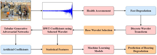
Figure 1. Flow chart of proposed methodology.

2. Materials and Method

2.1. Dataset

The FEMTO bearing dataset of prognostic and health management (PHM)’s IEEE challenge 2012, provided by the National Aeronautics and Space Administration (NASA) [27], is used. Figure 2 is an experimental setup of PRONOSTIA, used to test and validate the bearing’s fault detection and prognostics.

Figure 2. Overview of PRONOSTIA [27].

Table 1 shows the FEMTO bearing dataset generated by PRONOSTIA, which has acceleration values collected at a sampling frequency of 25.6 kHz as the data for a total of seventeen bearings, of which, seven were in condition 1 and 2, while three were in condition 3. In this study, the vibration data of six bearings operated at the radial load of 4000 N and 1800 rpm is used. Figure 3 shows the plot of the vibration signal against time for bearing 11 and bearing 13.

Table 1. FEMTO bearing dataset [27].

	Operating Condition
	Condition 1	Condition 2	Condition 3
Radial load (N)	4000	4200	5000
Speed (RPM)	1800	1650	1500
Dataset	Bearing11	Bearing21	Bearing31
	Bearing12	Bearing22	Bearing32
	Bearing13	Bearing23	Bearing33
	Bearing14	Bearing24
	Bearing15	Bearing25
	Bearing16	Bearing26
	Bearing17	Bearing27

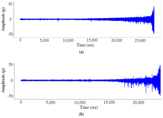
Figure 3. Vibration signal of (a) bearing 11 and (b) bearing 13 in the time domain.

2.2. Health Assessment

In this study, the complete bearing life was first divided into two health stages; the first was the normal degradation stage, while the second was the fast degradation stage, as shown in Figure 4 for all the bearing conditions, using a criterion, namely, singular value decomposition (SVD) normalized correlation coefficients, as proposed by Wentao Mao et al. [18]. The equation used to calculate the SVD normalized coefficient is

$$SV{D}_j=\frac{{{\displaystyle \sum }}_{i=1}^q{x}_i{y}_i}{\sqrt{{{\displaystyle \sum }}_{i=1}^q{x}_i^2{{\displaystyle \sum }}_{i=1}^q{y}_i^2}}$$

where x and y are the singular value vectors of the signal and j = 1 …N, q represents the length of singular value vectors.

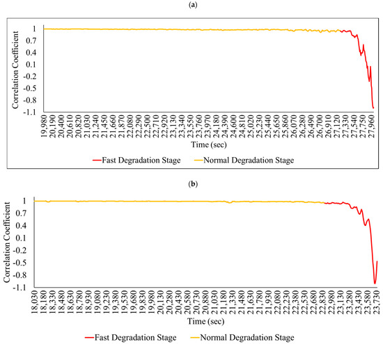
Figure 4. Health state of (a) bearing 11 and (b) bearing 13 [18].

As per Mao et al. [18], normal degradation and fast degradation can be identified on the basis of the correlation coefficient. If the correlation coefficient value lies consistently below 0.95, then it can be considered as being the bearing fast degradation state. The idea is to use the robustness of SVD, as with change, the correlation coefficient of SVD for the normal stage is comparatively higher than the correlation coefficient of SVD for the faulty stage. SVD also takes into account the noise, and minor deviations to the health assessment as the change in its value will be slight if the deviation is small, and if the signal varies greatly, it will show a large amount of change in its values. Thus, Wentao Mao et al. [18] concluded that the singular value decomposition (SVD) normalized correlation coefficient can be used to accurately find the change in a bearing’s health state when the vibration signal varies drastically.

2.3. Tabular Generative Adversarial Networks

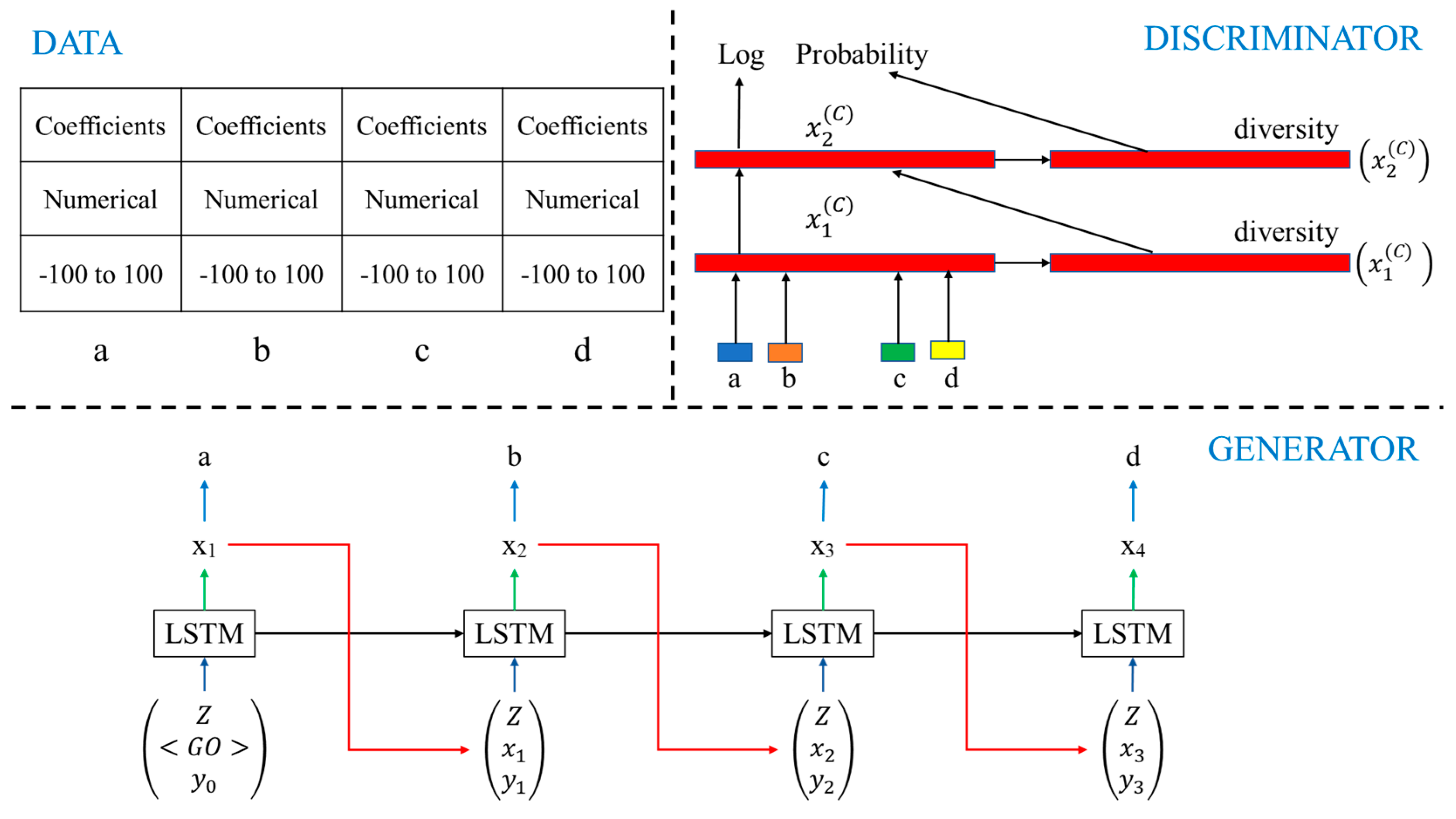
Machine learning algorithms require ample, adequate and reliable data, especially for unconventional and intricate applications performed by complex techniques [28,29]. For this study, collecting an ample amount of data was a major challenge, as collecting vibration data for the different parameters for different types of faults/defects is very time-consuming, costly and laborious. In recent years, GAN, i.e., generative adversarial networks, which were first developed by Goodfellow et al. [30], became a very popular and effective deep learning algorithm to generate feasible “fake data” from original data. Two neural networks, generator and discriminator, compete with each other in a min–max game, where the discriminator tries to identify the difference between the original data and the artificial data, while the generator tries to generate the artificial data in such a way that discriminator does not distinguish between the data. GANs are widely used to generate realistic and high-quality images in the field of computer vision. Various GANs such as the least squares GAN (LSGAN) [31], Wasserstein GAN (WGAN) [32], conditional GAN (CGAN) [33], information maximizing GAN (InfoGAN) [34], auxiliary classifier GAN (AC-GAN) [35], semi-supervised GAN (SGAN) [36], and tabular GANs (TGAN) [37] were developed and used for specific tasks, including fault detection, fraud detection, improving healthcare and improving cybersecurity [38]. In this study, tabular generative adversarial networks (TGAN), developed by Lei Xu and Kalyan Veeramachaneni [37], used a single table consisting of numerical as well as categorical variables to find the data distribution, to generate “fake data.” The synthetic table, T_synth, consists of continuous variables (C₁, C₂, C₃ ………, C_nr) with multinomial discrete random variables (D_mr1, D_mr2, D_mr3 ………, D_nr) and should follow a joint probability distribution and be sampled independently. The goal was to develop a generative model G (P C₁, P D_mr1) such that the sample generated represented a synthetic table T_synth which essentially resembled the original table, with slight variations. In this study, the authors have used 100 hidden units and 100 hidden layers to characterize LSTM cells.

As observed in Figure 5, the generator was developed using a long short-term memory (LSTM) neural network with a hidden vector $x_t=\tanh \left(V_t{k}_i\right)$, where $k_i$ was the output of LSTM and $V_t$ was the learned parameter in the network. The input to the LSTM was the random noise z, the hidden vector x and the weight vector y. The output was calculated as $a_i=b_i=c_i=\mathrm{softmax}\left(V_t{x}_t\right)$ for discrete variables. A cross-entropy loss, along with KL divergence, was used as a loss function. For the discriminator, a multi-layer perceptron (MLP), an n-layer fully connected neural network, was used, and a_1:n, b_1:n and c_1:n were fed in a concatenated manner. The first layer and the ith layer were calculated as,

$$x_1=\mathrm{LeakyReLU}\left(\mathrm{BN}\left(V_1^{\left(C\right)}\left(a_{1:n}\oplus b_{1:n}\oplus c_{1:n}\right)\right)\right)$$

(1)

$$x_i=\mathrm{LeakyReLU}\left(\mathrm{BN}\left(V_i^{\left(C\right)}\left(x_{i-1}^{\left(C\right)}\oplus \mathrm{diversity}\left(x_{i-1}^{\left(C\right)}\right)\right)\right)\right),i=2:n$$

(2)

where ⊕ is the concatenation operator, diversity is the mini-batch discrimination vector, BN is batch normalization, and Leaky ReLU is the activation function. A conventional cross-entropy loss was used as a loss function. In this study, the artificial coefficients of the DWT were generated using TGAN.

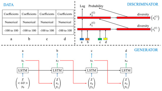
Figure 5. TGAN architecture.

2.4. Feature Extraction

Non-linearity is generally observed when a vibration signal is captured using the sensors from a bearing, as noise can be generated either due to surrounding environmental conditions or by faults in the bearing itself. Thus, it becomes very important to select appropriate signal processing techniques to extract useful information (features) about the health stage of the bearing. Three types of features can be extracted from captured vibration signals; time–domain features, frequency–domain features and time–frequency–domain features. Time–domain statistical features are extracted from the time waveforms of the captured vibration signals of the bearing [39,40,41]. In the current study, 13 time–domain statistical features including the mean, sum and skewness, were calculated from original db1 wavelet coefficients and the coefficients generated by TGAN. The equations used to calculate the feature vectors are shown in Table 2.

Table 2. Equations of Statistical Time-Domain Features.

Name	Description	Formula
Mean	The average value of the vibration signal	$x_m=\frac{1}{K}\ast {\displaystyle {\displaystyle \sum }_{k=1}^K}x\left(k\right)$	(3)
Standard Deviation	Deviation from the mean value of the vibration signal	$x_{std}=\sqrt{\frac{{{\displaystyle \sum }}_{k=1}^K{\left(x\left(k\right)-x_m\right)}^2}{\left(K-1\right)}}$	(4)
Variance	Square of standard deviation	$x_{var}=\frac{{{\displaystyle \sum }}_{k=1}^K{\left(x\left(k\right)-x_m\right)}^2}{\left(K-1\right)}$	(5)
Sum	Sum of signal	$Sum={\displaystyle {\displaystyle \sum }_{k=1}^K}x\left(k\right)$	(6)
Skewness	A measure of lack of symmetry	$x_{skew}=\frac{{{\displaystyle \sum }}_{k=1}^K{\left(x\left(k\right)-x_m\right)}^3}{\left(K-1\right)\hspace{1em}\ast \hspace{1em}{x}_{std}^3}$	(7)
Kurtosis	A measure of the spikiness of the signal relative to a normal distribution	$x_{kurt}=\frac{{{\displaystyle \sum }}_{k=1}^K{\left(x\left(k\right)-x_m\right)}^4}{\left(K-1\right)\hspace{1em}\ast \hspace{1em}{x}_{std}^4}$	(8)
Root Mean Square (RMS)	The square root of the mean of squares of a signal	$x_{rms}={\displaystyle {\displaystyle \sum }_{k=1}^K}\frac{{\left(x\left(k\right)\right)}^2}{K}$	(9)
Peak to Peak Value	Difference between maximum and minimum peak values	$x_{ppv}=x_{max}-x_{min}$	(10)
Maximum Amplitude	Value of the maximum amplitude of the signal	$x_{max}=max(x\left(k\right)$)	(11)
Minimum Amplitude	Value of the minimum amplitude of the signal	$x_{min}=min(x\left(k\right)$)	(12)
Crest Factor	The ratio of peak value to RMS value	$x_{CF}=\frac{x_{max}}{x_{rms}}$	(13)
Shape Factor	The ratio of RMS value and mean-value	$x_{SF}=\frac{x_{rms}}{x_m}$	(14)
Impulse Factor	The ratio of max value and mean value	$x_{IF}=\frac{x_{max}}{x_m}$	(15)

2.5. Machine Learning Models

2.5.1. Ensemble Bagged Trees

Ensemble methods utilize the combination of several decision trees so as to obtain better predictions, as compared to single tree classifiers. The core idea behind the building of an ensemble model is that a set of weak learners join together to become a strong learner. As a result, we have a collection of various models and the average of all predictions from various trees is utilized, which is more reliable than a single decision tree classifier. In EBT, bagging is applied to minimize the variance in the decision tree classifier. There are N readings and F features in a feature vector, and a subset of M features are selected, and the feature which gives the best split is chosen to split the nodes iteratively. The procedure is repeated N times, and a prediction is made based on the sum of predictions from N trees. In Figure 6, the color represents the various extracted features applied for training, testing and cross-validation of ML models.

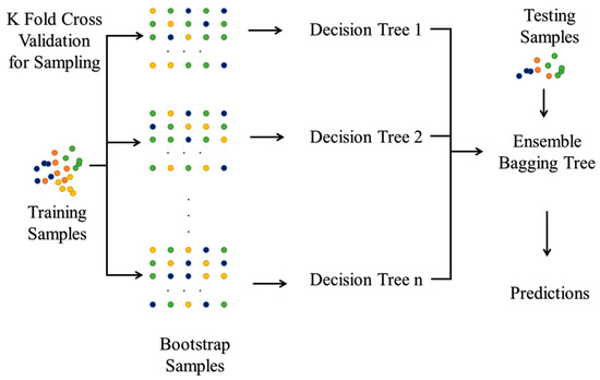
Figure 6. Ensemble Bagging Tree.

2.5.2. Squared Exponential Gaussian Processes Regression (SEGPR)

This method is one of the supervised learning algorithms specifically designed to solve the regression problem. Usually, the calculation of the probability distribution is carried on a specific function, but in Gaussian processes regression, the probability distribution is calculated by fitting the data over all the functions. In this study, the squared exponential kernel (exponentiated quadratic or radial basis function) was used with Gaussian processes regression as it is infinitely differentiable, which states that if used as a covariance function, then it will be very smooth as it includes mean square derivatives of all orders [42,43]. It is based on equations such as

$$s\left(u_i,u_j\right)={\sigma }_{std}^2{e}^{\left[-\frac{1}{2}\frac{\Vert u_i-u_j\Vert {}^2}{{\sigma }_{lc}^2}\right]}$$

(16)

where ${\sigma }_{lc}$ is the characteristic length scale, ${\sigma }_{std}$ is the standard deviation of the signal and u_i, and u_j denotes the value of the signal at location i and j.

3. Results and Discussions

Features extracted using the wavelet transform are very useful in detecting abrupt variations in the captured vibration signals. Due to the development and vast availability of the several base functions of the wavelet, it is advantageous to use them to identify the degradation of the bearing [40]. It is very important to select the appropriate base function to extract features of the captured vibration signals [44]. Discrete wavelet transform is performed as it is one of the best tools for signal analysis and signal processing, such as noise reduction and data compression. A technique known as mutual information (MI) [45], which measures the dependency between two variables, was used in this study to select the appropriate base function for DWT-based feature extraction. Mutual information (MI) measures the dependency between two variables, which is given by the equation

MI·(X;Y) = E(X) − CE(X|Y)

(17)

where MI·(X;Y) is the mutual information for X and Y, E(X) is the entropy for X and CE (X|Y) is the conditional entropy for X given Y, and X and Y are the variables.

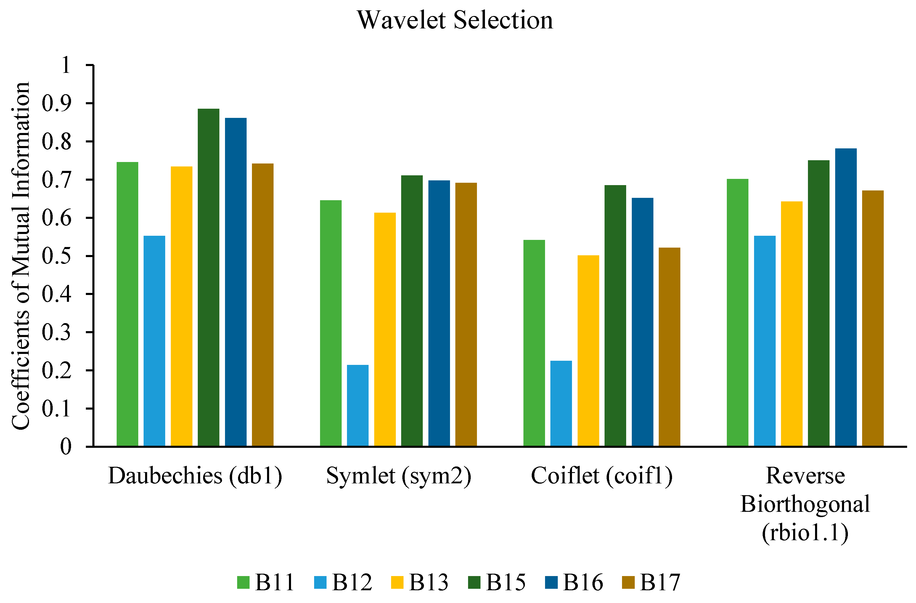
A function is selected as a base function when MI shows the maximum amount of dependency. In this study, the base functions of wavelets compared were Daubechies (db1), Symlet (sym2), Coiflet (coif1), and reverse Biorthogonal (rbio1.1). All six bearings were considered at a speed of 1800 rpm and a load of 4000 N to select the base function of the wavelet. It is clear from Figure 7 that Daubechies (db1) shows the highest MI as compared to other wavelets functions, and was therefore selected to calculate DWT-based statistical features.

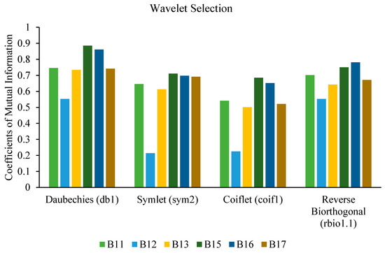
Figure 7. Wavelet selection based on mutual information.

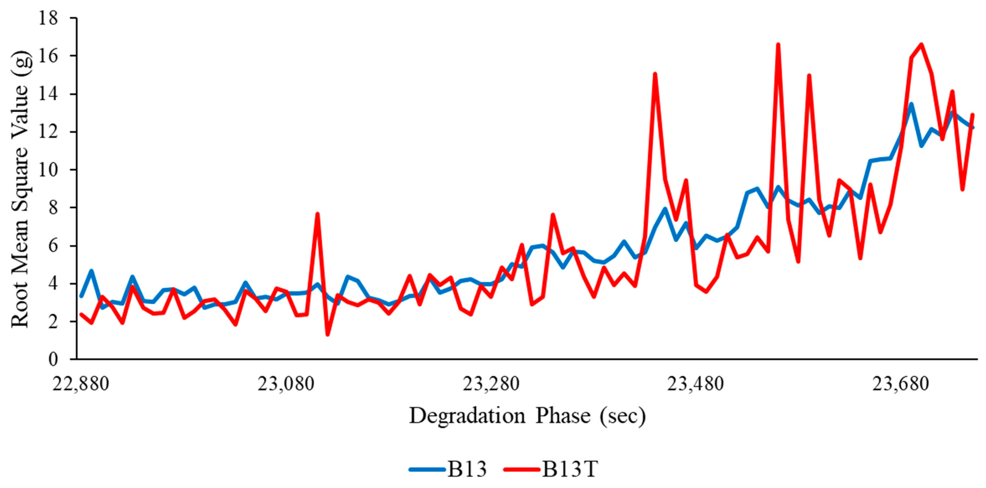
Availability of experimental data is critical for building machine-learning-based degradation models to better understand the non-linear connection between various extracted statistical features. Considering the availability of small size datasets, the small amount of data provided for testing raises concerns about the effectiveness of ML models accuracy, therefore, the authors have proposed a novel architecture: a tabular generative adversarial network (TGAN) for enhancing the dataset, which in turn can be useful for improving accuracy, robustness, and generalisation capabilities for future experimental data which is previously unknown to the developed model. Figure 8 shows the sample root mean square value between real and artificial data generated through TGAN. It can be observed that there were very slight variations in the RMS values between actual experimental data and the generated data. Furthermore, this shows the utility of generated features through TGAN, and Table 3 compares the statistical properties of the actual features to those of the generated features. As can be seen from Table 3, there were slight deviations in the statistical parameters for the real features and generated features.

Figure 8. Real vs. artificial root mean square values for B13.

Table 3. Statistical comparison of real features and generated features.

	Mean	Mean	Std	Std	Var	Var	RMS	RMS
	Original Features	Generated Features	Original Features	Generated Features	Original Features	Generated Features	Original Features	Generated Features
Mean	0.048	0.058	5.863	5.22	42.744	42.985	5.869	5.855
Std	0.381	0.351	2.908	2.887	43.260	43.842	2.915	2.896
Min	2.205	1.986	2.730	3.442	7.4578	6.987	2.730	2.425
25	0.033	0.092	3.455	3.885	11.937	11.845	3.454	3.198
50	0.010	0.012	4.950	5.441	24.513	23.854	4.955	4.287
75	0.088	0.089	7.930	8.661	62.901	61.825	7.984	7.511
Max	0.852	0.885	13.479	13.479	181.68	181.68	13.475	13.47
	Max	Max	Min	Min	P2P	P2P	Skew	Skew
	Original Features	Generated Features	Original Features	Generated Features	Original Features	Generated Features	Original Features	Generated Features
Mean	26.376	26.88	34.254	33.158	60.630	58.251	0.624	0.584
Std	13.575	13.896	13.029	12.586	24.980	23.420	0.566	0.486
Min	11.343	11.969	63.257	62.884	24.224	23.884	3.076	2.871
25	15.799	15.966	44.578	43.857	41.883	40.458	0.843	0.824
50	21.854	22.236	31.44	30.548	51.500	50.898	0.575	0.564
75	34.472	36.001	24.029	22.885	81.257	80.750	0.259	0.249
Max	68.063	69.012	12.881	13.987	131.32	131.32	0.524	0.514
	Kurt	Kurt	SF	SF	IF	IF	CF	CF
	Original Features	Generated Features	Original Features	Generated Features	Original Features	Generated Features	Original Features	Generated Features
Mean	9.084	8.854	1.467	1.384	6.672	6.445	4.539	4.586
Std	4.088	3.475	0.085	0.076	1.168	1.075	0.713	0.816
Min	3.292	2.745	1.269	1.148	4.189	4.096	3.191	3.091
25	6.293	6.110	1.413	1.388	5.957	5.348	4.043	4.055
50	7.888	7.550	1.463	1.446	6.571	6.412	4.388	4.281
75	10.742	10.314	1.529	1.498	7.525	7.539	5.047	4.889
Max	25.546	250.546	1.700	1.622	10.024	10.024	6.331	5.996

In the current study, two ML models were used to evaluate the degradation of six bearings conditions. Initially, training was executed using the real and generated feature vectors, and afterwards, five-fold cross-validation, ten-fold cross-validation and fifteen-fold cross-validation were performed on ML models. Cross-validation is a resampling procedure which is used to evaluate machine learning models, so that bias and overfitting can be avoided and generalization capability can be improved. In five-fold cross-validation, datasets are first divided in to five equal parts, and for the first fold, one part is used for testing and the other four parts are used for training. In the second fold, two parts are used for testing and three parts are used for training. The procedure repeats for the rest of the portions and the predictions are generated after averaging all folds. In the present study, for five-fold, ten-fold and fifteen-fold cross-validation, mean RMSE and MAE were computed after applying EBT and SEGPR models.

Two performance metrics, the root mean square error (RMSE) and mean absolute error (MAE), are considered to evaluate the performance of ML models for the predictions of bearing degradation. Performance metrics were calculated as follows:

3.1. Mean Absolute Error (MAE)

The World Bankreflects the average deviation obtained from the differences between the experimental/calculated values and the predicted values [41]. It is represented by the equation:

$$MAE=\frac{1}{N}{\displaystyle \sum }_{i=0}^N\left|{\widehat{y}}_i-y\right|$$

(18)

where ${\widehat{y}}_i$ represents the predicted values obtained using ML models, while y shows the experimental/calculated values.

3.2. Root Mean Square Error (MAE)

RMSE is the square root of the mean of the squared difference between the experimental/calculated values and the predicted values. It is a significant parameter widely used to evaluate the performance of regressions model and is represented mathematically as:

$$RMSE=\sqrt{\frac{1}{N}{\displaystyle \sum }_{i=0}^N{\left({\widehat{y}}_i-y\right)}^2}$$

(19)

where ${\widehat{y}}_i$ represents the predicted values obtained using ML models, while y shows the experimental/calculated values.

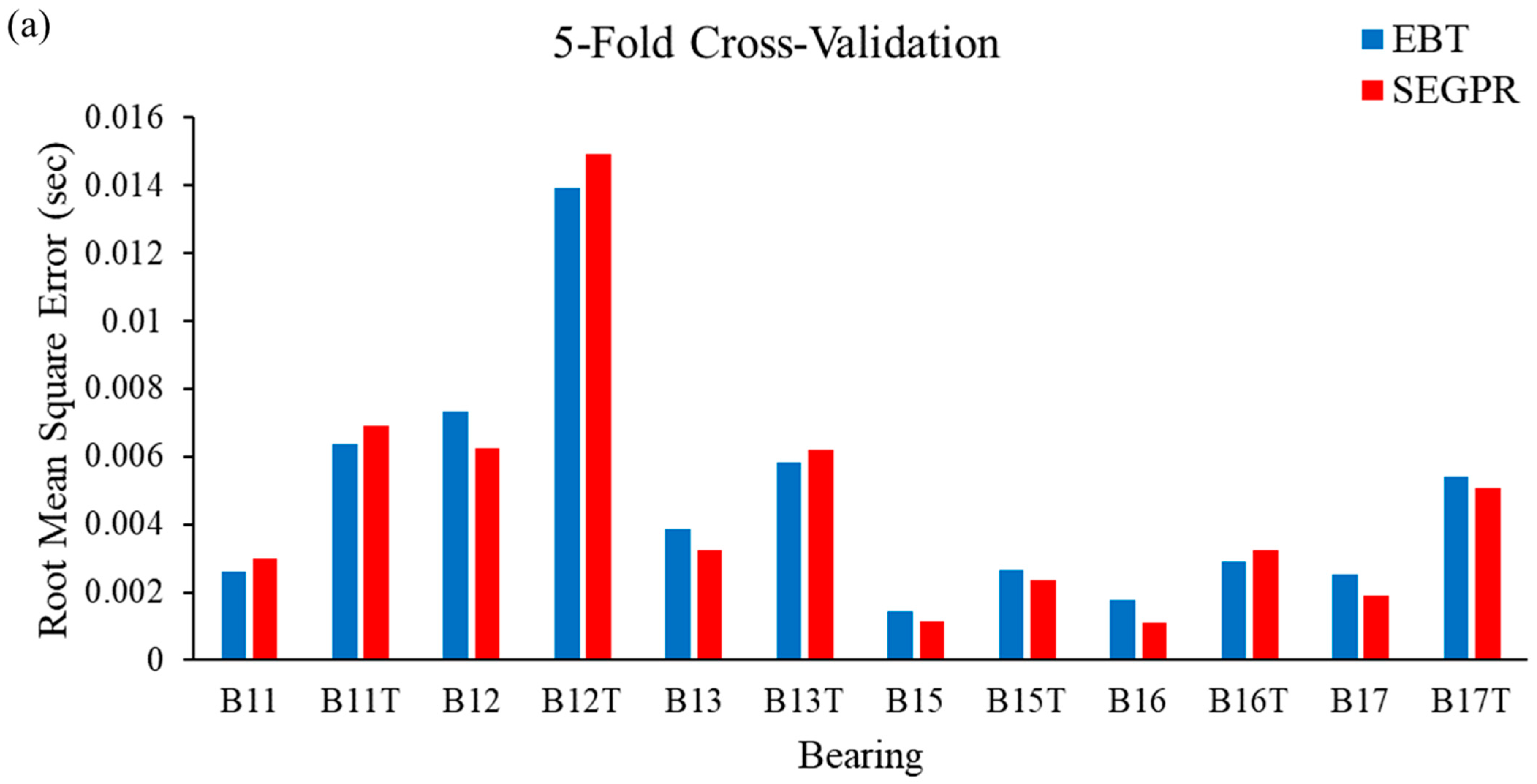
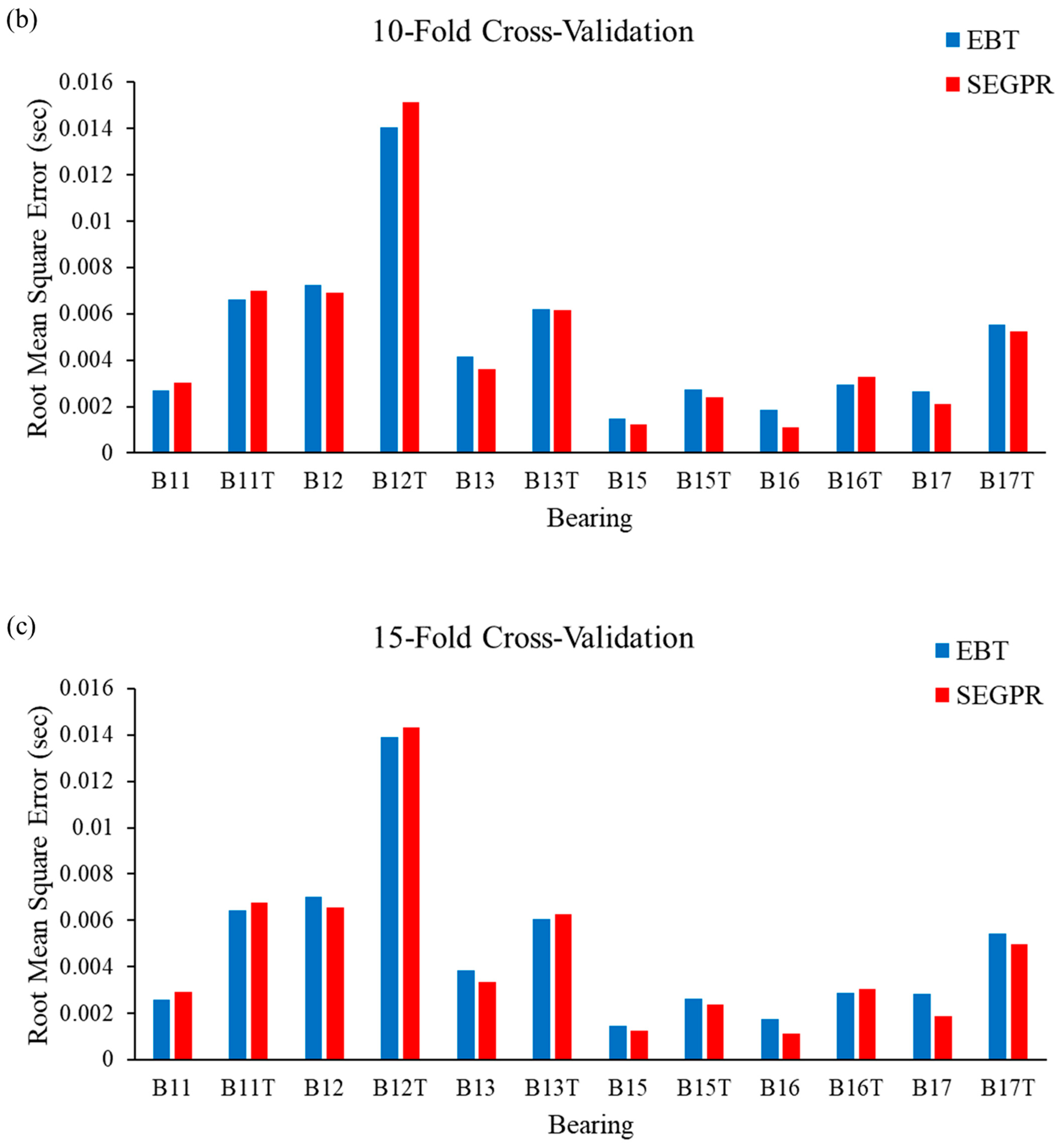
In this study, bearing degradation was predicted using two machine learning algorithms; namely, ensemble bagged tree (EBT) and squared exponential Gaussian processes regression (SEGPR), for the features extracted through actual experimental data and the artificial data generated by TGAN. It was observed that the feature vector was randomly split into training and testing. To avoid bias as well as to minimize misclassification errors, the authors have implemented k-fold cross-validation techniques. RMSE and MAE have been calculated after applying five-fold cross-validation, ten-fold cross-validation and fifteen-fold cross-validation procedures in ML models. Figure 9a–c shows the RMSE obtained when EBT and SEGPR models are applied with five-fold cross-validation, ten-fold cross-validation and fifteen-fold cross-validation procedures, respectively. From Figure 9a, it can be seen that the performance of the SEGPR model was better than the EBT model, as the average RMSE value for all the bearing degradation conditions, as well as original and generated data, was 0.0046, as compared to 0.0047 with the EBT model. Figure 9b represents the average RMSE value obtained after applying EBT and SEGPR models with ten-fold cross-validation. The average RMSE value obtained after applying ML models were 0.0047 and 0.0048 with SEGPR and EBT models, respectively. Similarly, the average RMSE value obtained after applying ML models were 0.0045 and 0.0047 with SEGPR and EBT models, respectively. Figure 9c shows when a fifteen-fold cross validation procedure was applied. It can be seen that the SEGPR model predicted bearing degradation better than the EBT model with original and generated bearing degradation data, as well as for all cross-validation conditions.

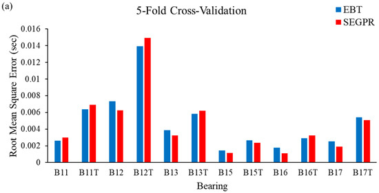
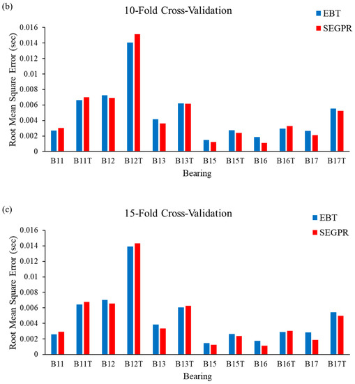
Figure 9. (a–c). RMSE values observed from the EBT and SEGPR ML models.

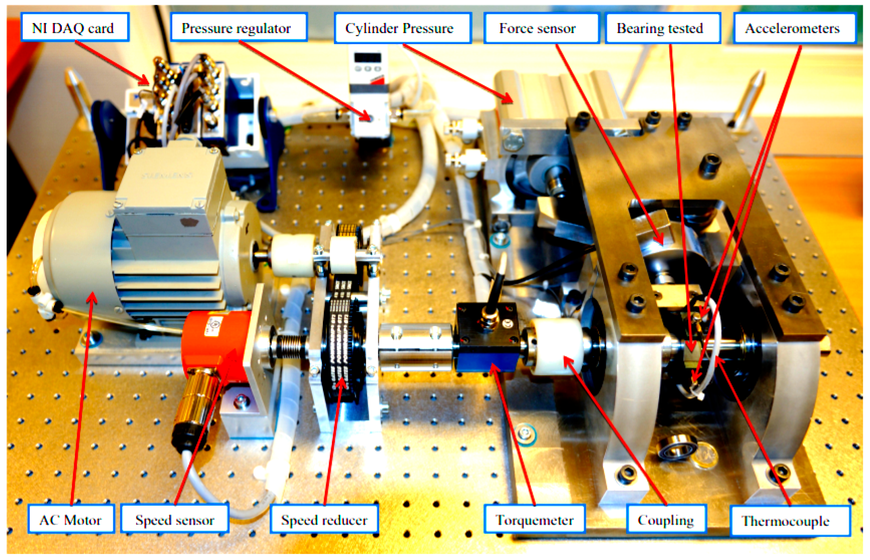
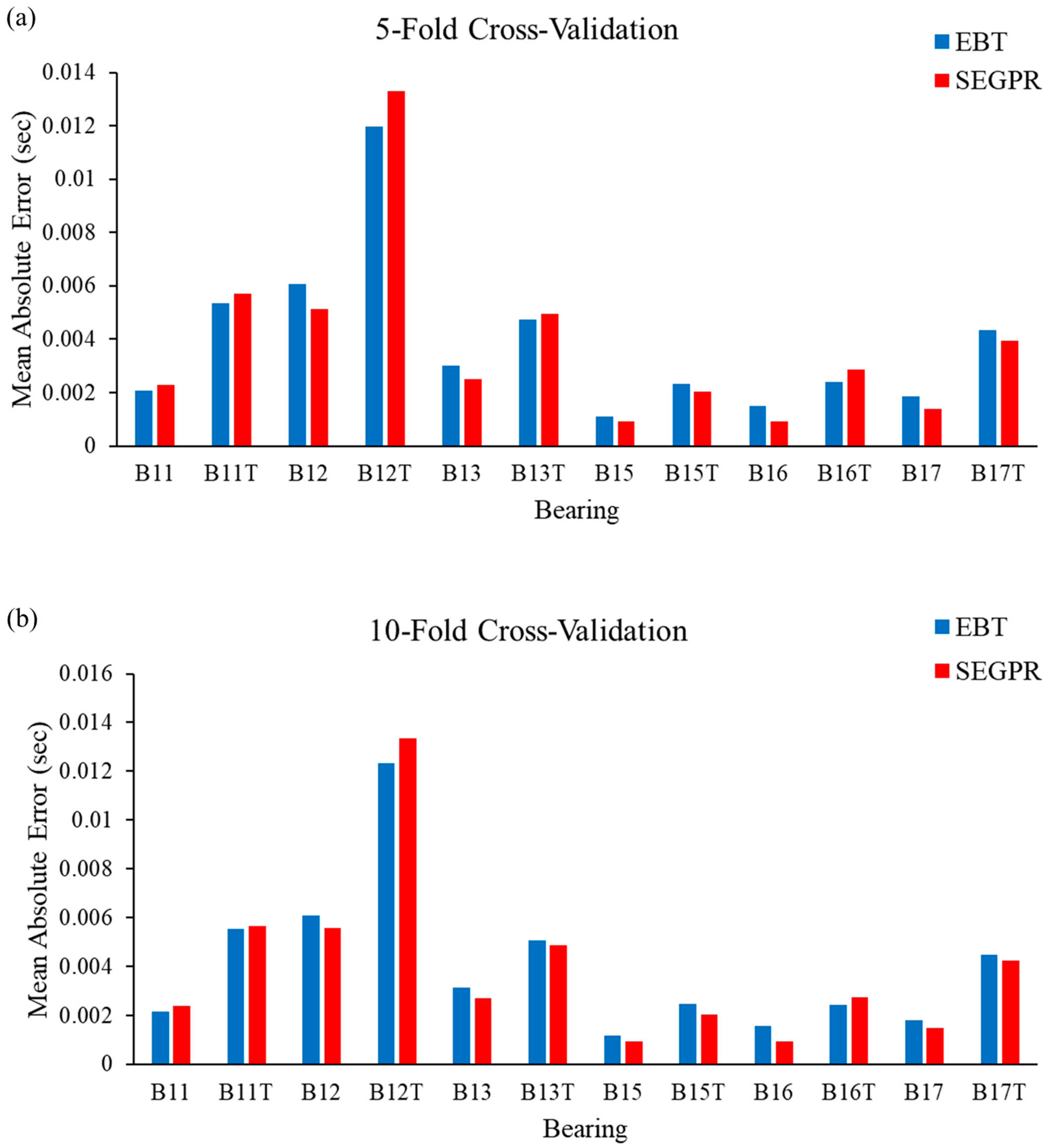
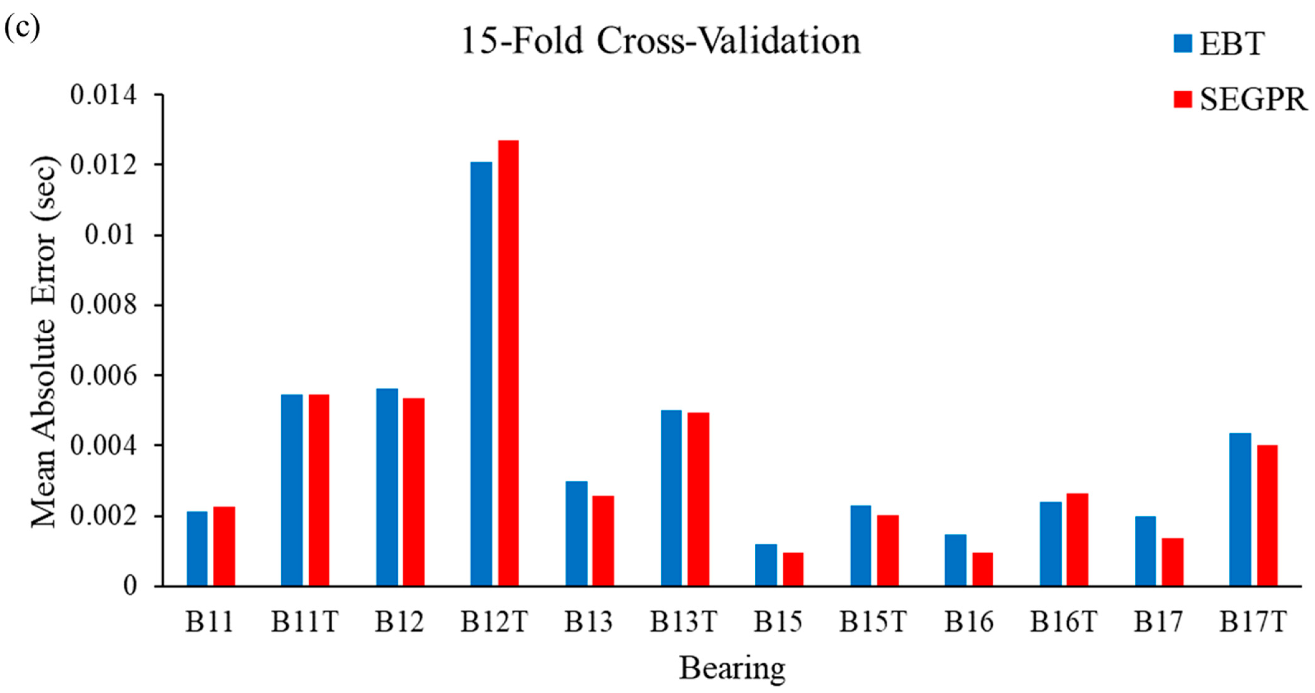
To justify the utility of the proposed methodology, MAE values were calculated and plotted, which can be observed in Figure 10a–c. From Figure 10a, it can be seen that the performance of the SEGPR model was better than the EBT model, as the average MAE value for all the bearing degradation conditions, as well as original and generated data, was 0.0038, as compared to 0.0039 with the EBT model. Figure 10b represents the average MAE value obtained after applying the EBT and SEGPR models with ten-fold cross-validation. The average MAE values obtained after applying ML models were 0.0039 and 0.0040 with SEGPR and EBT models, respectively. Similarly, the average MAE values obtained after applying ML models were 0.0037 and 0.0039 with SEGPR and EBT models, respectively. Figure 10c shows when a fifteen-fold cross validation procedure was applied. It can be seen that, once again, the SEGPR model predicted bearing degradation better than the EBT model, based on MAE performance metrics. It should be noted that all the RMSE and MAE values were very small and were under the permissible limit of industry and research conditions. One of the reasons for the better performance of the SEGPR model is that the kernel function squared exponential is infinitely differentiable, which generates a smooth curve, which enables the easy fitting of the data. To verify the effectiveness of the proposed methodology, a comparison table with the previously published literature, Table 4, was prepared, in which different authors have used the same bearing degradation dataset. It can be seen that with smaller datasets, the prediction results are comparatively better than when TGAN is utilized with wavelet transform and the SEGPR model.

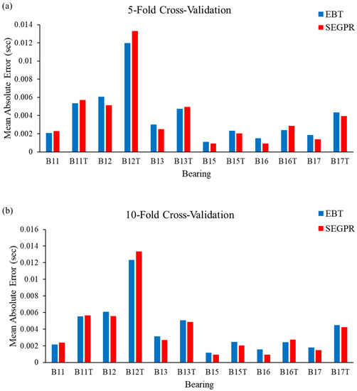
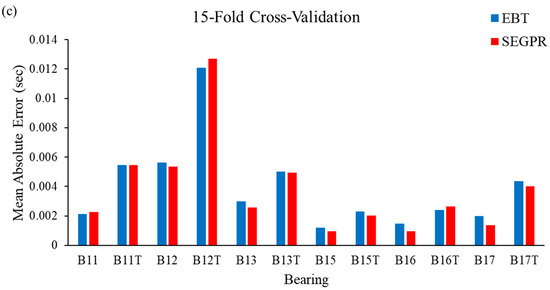
Figure 10. (a–c). MAE values observed from the EBT and SEGPR ML models.

Table 4. A comparative study between current work and previously published papers to predict bearing degradation using different ML models.

References	Model	Dataset	MAE	RMSE
Xiang Li et al. [15]	CNN	17	19.65882	23.61765
Wentao Mao et al. [18]	CNN + LSTM	4	-	80
David Verstraete et al. [25]	Adversarial–Variational Model	3	-	8.173333
Xiang Li et al. [26]	GAN + CNN	17	-	34.05882
Jehn-Ruey Jiang et al. [46]	TSMC + CNN + ALSTM	-	0.0186	0.0268
Qiming Niu et al. [47]	NARX	6	1.60	2.94
Proposed	TGAN + SEGPR	6	0.00225 (Real)	0.00285 (Real)
			0.00529 (Artificial)	0.00629 (Artificial)

4. Conclusions

In the current study, the bearing degradation of six bearings computed from original data and artificial data generated using TGAN has been predicted using two machine learning models: ensemble bagged tree (EBT) and squared exponential Gaussian processes regression (SEGPR). Initially, the raw vibration signals were captured and pre-processed using the selected DWT functions based on the MI criterion. Thirteen statistical features were calculated, and to demonstrate the utility of TGAN for degradation prediction, an artificial feature vector was generated. After applying two ML models with five-, ten- and fifteen-fold cross-validation, observations were as follows:

• The effectiveness of ML models was assessed with two standard performance metrics: RMSE and MAE. Least errors have been observed to predict bearing degradation from both the EBT and SEGPR models.
• The lowest RMSE value of 0.0045 was observed with the SEGPR model when fifteen-fold cross-validation was implemented, whereas with the EBT model, the lowest RMSE was observed as 0.0047 when five-fold cross-validation was implemented.
• With the SEGPR model, the lowest MAE value observed was 0.0037 when fifteen-fold cross-validation was implemented, whereas with the EBT model, the lowest MAE was observed as 0.0038 with five-fold cross-validation.
• The methodology developed based on hybrid TGAN–SEGPR, which is least explored for bearing degradation, can be useful to various applications including fault diagnosis, fault severity, and manufacturing parameter assessments, when the availability of experimental data is limited, which makes difficult to develop ML models.

Authors expect that the additional data generated through TGAN will be extremely useful in a variety of interdisciplinary applications, for classification, as well as regression analysis, with ML models.

References

- Heng, A.; Zhang, S.; Tan, A.C.; Mathew, J. Rotating machinery prognostics: State of the art, challenges and opportunities. Mech. Syst. Signal Process. 2009, 23, 724–739. [Google Scholar] [CrossRef]
- Lee, J.; Wu, F.; Zhao, W.; Ghaffari, M.; Liao, L.; Siegel, D. Prognostics and health management design for rotary machinery systems—Reviews, methodology and applications. Mech. Syst. Signal Process. 2014, 42, 314–334. [Google Scholar] [CrossRef]
- Kankar, P.K.; Sharma, S.C.; Harsha, S.P. Fault diagnosis of ball bearings using machine learning methods. Expert Syst. Appl. 2011, 38, 1876–1886. [Google Scholar] [CrossRef]
- Vakharia, V.; Gupta, V.; Kankar, P. Nonlinear dynamic analysis of ball bearings due to varying number of balls and centrifugal force. In Proceedings of the 9th IFToMM International Conference on Rotor Dynamics; Springer: Milan, Italy, 2015; pp. 1831–1840. [Google Scholar]
- Benkedjouh, T.; Medjaher, K.; Zerhouni, N.; Rechak, S. Remaining useful life estimation based on nonlinear feature reduction and support vector regression. Eng. Appl. Artif. Intell. 2013, 26, 1751–1760. [Google Scholar] [CrossRef]
- Qiu, H.; Lee, J.; Lin, J.; Yu, G. Robust performance degradation assessment methods for enhanced rolling element bearing prognostics. Adv. Eng. Inform. 2003, 17, 127–140. [Google Scholar] [CrossRef]
- Albrecht, P.; Appiarius, J.; McCoy, R.; Owen, E.; Sharma, D. Assessment of the reliability of motors in utility applications-Updated. IEEE Trans. Energy Convers. 1986, EC-1, 39–46. [Google Scholar] [CrossRef]
- Lei, Y.; Li, N.; Gontarz, S.; Lin, J.; Radkowski, S.; Dybala, J. A model-based method for remaining useful life prediction of machinery. IEEE Trans. Reliab. 2016, 65, 1314–1326. [Google Scholar] [CrossRef]
- Omoregbee, H.O.; Heyns, P.S. Fault classification of low-speed bearings based on support vector machine for regression and genetic algorithms using acoustic emission. J. Vib. Eng. Technol. 2019, 7, 455–464. [Google Scholar] [CrossRef]
- Jardine, A.K.; Lin, D.; Banjevic, D. A review on machinery diagnostics and prognostics implementing condition-based maintenance. Mech. Syst. Signal Process. 2006, 20, 1483–1510. [Google Scholar] [CrossRef]
- Bustillo, A.; Pimenov, D.Y.; Matuszewski, M.; Mikolajczyk, T. Using artificial intelligence models for the prediction of surface wear based on surface isotropy levels. Robot. Comput.-Integr. Manuf. 2018, 53, 215–227. [Google Scholar] [CrossRef]
- Dave, V.; Singh, S.; Vakharia, V. Diagnosis of bearing faults using multi fusion signal processing techniques and mutual information. Indian J. Eng. Mater. Sci. 2021, 27, 878–888. [Google Scholar]
- Akhenia, P.; Bhavsar, K.; Panchal, J.; Vakharia, V. Fault severity classification of ball bearing using SinGAN and deep convolutional neural network. Proc. Inst. Mech. Eng. Part C J. Mech. Eng. Sci. 2021. [Google Scholar] [CrossRef]
- Chen, Y.; Li, Y.; An, W.; Liu, H.; Jiang, T. Rolling Bearing Performance Degradation Prediction Based on FBG Signal. IEEE Sens. J. 2021, 21, 24134–24141. [Google Scholar] [CrossRef]
- Li, X.; Zhang, W.; Ding, Q. Deep learning-based remaining useful life estimation of bearings using multi-scale feature extraction. Reliab. Eng. Syst. Saf. 2019, 182, 208–218. [Google Scholar] [CrossRef]
- Zhu, J.; Chen, N.; Peng, W. Estimation of bearing remaining useful life based on multiscale convolutional neural network. IEEE Trans. Ind. Electron. 2018, 66, 3208–3216. [Google Scholar] [CrossRef]
- Behzad, M.; Arghand, H.A.; Rohani Bastami, A. Remaining useful life prediction of ball-bearings based on high-frequency vibration features. Proc. Inst. Mech. Eng. Part C J. Mech. Eng. Sci. 2018, 232, 3224–3234. [Google Scholar] [CrossRef]
- Mao, W.; He, J.; Tang, J.; Li, Y. Predicting remaining useful life of rolling bearings based on deep feature representation and long short-term memory neural network. Adv. Mech. Eng. 2018, 10. [Google Scholar] [CrossRef]
- Yoo, Y.; Baek, J.-G. A novel image feature for the remaining useful lifetime prediction of bearings based on continuous wavelet transform and convolutional neural network. Appl. Sci. 2018, 8, 1102. [Google Scholar] [CrossRef] [Green Version]
- Wang, B.; Lei, Y.; Li, N.; Li, N. A hybrid prognostics approach for estimating remaining useful life of rolling element bearings. IEEE Trans. Reliab. 2018, 69, 401–412. [Google Scholar] [CrossRef]
- Ye, X.; Li, G.; Meng, L.; Lu, G. Dynamic health index extraction for incipient bearing degradation detection. ISA Trans. 2021. [Google Scholar] [CrossRef]
- Savić, B.; Urošević, V.; Ivković, N.; Popović, M.; Gubeljak, N.; Šiniković, G. Implementation of a Non-Linear Regression Model in Rolling Bearing Diagnostics. Teh. Vjesn. 2022, 29, 314–321. [Google Scholar]
- Blaut, J.; Breńkacz, Ł. Application of the Teager-Kaiser energy operator in diagnostics of a hydrodynamic bearing. Eksploat. I Niezawodn. 2020, 22, 757–765. [Google Scholar] [CrossRef]
- Kubik, A.; Stanik, Z.; Hadryś, D.; Csiszár, C. Impact of Selected Operational Parameters on Measures of Technical Condition of Rolling Bearings in Means of Transport Built Based on Analysis of Vibration Signals. Sci. J. Silesian Univ. Technol. Ser. Transp. 2021, 111, 89–98. [Google Scholar] [CrossRef]
- Verstraete, D.; Droguett, E.; Modarres, M. A deep adversarial approach based on multi-sensor fusion for semi-supervised remaining useful life prognostics. Sensors 2020, 20, 176. [Google Scholar] [CrossRef] [PubMed] [Green Version]
- Li, X.; Zhang, W.; Ma, H.; Luo, Z.; Li, X. Data alignments in machinery remaining useful life prediction using deep adversarial neural networks. Knowl.-Based Syst. 2020, 197, 105843. [Google Scholar] [CrossRef]
- Nectoux, P.; Gouriveau, R.; Medjaher, K.; Ramasso, E.; Chebel-Morello, B.; Zerhouni, N.; Varnier, C. PRONOSTIA: An experimental platform for bearings accelerated degradation tests. In Proceedings of the IEEE International Conference on Prognostics and Health Management, PHM’12, Denver, CO, USA, 18–21 June 2012; pp. 1–8. [Google Scholar]
- Bustillo, A.; Pimenov, D.Y.; Mia, M.; Kapłonek, W. Machine-learning for automatic prediction of flatness deviation considering the wear of the face mill teeth. J. Intell. Manuf. 2021, 32, 895–912. [Google Scholar] [CrossRef]
- Bustillo, A.; Reis, R.; Machado, A.R.; Pimenov, D.Y. Improving the accuracy of machine-learning models with data from machine test repetitions. J. Intell. Manuf. 2020, 1–19. [Google Scholar] [CrossRef]
- Goodfellow, I.; Pouget-Abadie, J.; Mirza, M.; Xu, B.; Warde-Farley, D.; Ozair, S.; Courville, A.; Bengio, Y. Generative adversarial nets. In Proceedings of the Advances in Neural Information Processing Systems, Montreal, QC, Canada, 8–13 December 2014; Volume 27. [Google Scholar]
- Mao, X.; Li, Q.; Xie, H.; Lau, R.Y.; Wang, Z.; Paul Smolley, S. Least squares generative adversarial networks. In Proceedings of the IEEE International Conference on Computer Vision, Venice, Italy, 22–29 October 2017; pp. 2794–2802. [Google Scholar]
- Arjovsky, M.; Chintala, S.; Bottou, L. Wasserstein generative adversarial networks. In Proceedings of the International Conference on Machine Learning, Sydney, NSW, Australia, 11 August 2017; pp. 214–223. [Google Scholar]
- Mirza, M.; Osindero, S. Conditional generative adversarial nets. arXiv 2014, arXiv:1411.1784. Available online: https://arxiv.org/abs/1411.1784 (accessed on 26 January 2022).
- Chen, X.; Duan, Y.; Houthooft, R.; Schulman, J.; Sutskever, I.; Abbeel, P. Infogan: Interpretable representation learning by information maximizing generative adversarial nets. In Proceedings of the 30th International Conference on Neural Information Processing Systems, Barcelona, Spain, 5–10 December 2016; pp. 2180–2188. [Google Scholar]
- Odena, A.; Olah, C.; Shlens, J. Conditional image synthesis with auxiliary classifier gans. In Proceedings of the International Conference on Machine Learning, Sydney, NSW, Australia, 10 April 2017; pp. 2642–2651. [Google Scholar]
- Odena, A. Semi-supervised learning with generative adversarial networks. arXiv 2016, arXiv:1606.01583. Available online: https://arxiv.org/abs/1606.01583 (accessed on 26 January 2022).
- Xu, L.; Veeramachaneni, K. Synthesizing tabular data using generative adversarial networks. arXiv 2018, arXiv:1811.11264. Available online: https://arxiv.org/abs/1811.11264 (accessed on 26 January 2022).
- Zheng, Y.-J.; Zhou, X.-H.; Sheng, W.-G.; Xue, Y.; Chen, S.-Y. Generative adversarial network based telecom fraud detection at the receiving bank. Neural Netw. 2018, 102, 78–86. [Google Scholar] [CrossRef] [PubMed]
- Malla, C.; Panigrahi, I. Review of condition monitoring of rolling element bearing using vibration analysis and other techniques. J. Vib. Eng. Technol. 2019, 7, 407–414. [Google Scholar] [CrossRef]
- Vakharia, V.; Gupta, V.; Kankar, P. Efficient fault diagnosis of ball bearing using ReliefF and Random Forest classifier. J. Braz. Soc. Mech. Sci. Eng. Appl. Artif. Intell. 2017, 39, 2969–2982. [Google Scholar] [CrossRef]
- Upadhyay, R.; Padhy, P.; Kankar, P. A comparative study of feature ranking techniques for epileptic seizure detection using wavelet transform. Comput. Electr. Eng. 2016, 53, 163–176. [Google Scholar] [CrossRef]
- Duvenaud, D. Automatic Model Construction with Gaussian Processes. Ph.D. Thesis, University of Cambridge, Cambridge, UK, 2014. [Google Scholar]
- Rasmussen, C.E.; Williams, C.K. Gaussian Processes for Machine Learning; The MIT Press: Cambridge, UK, 2006. [Google Scholar]
- Vakharia, V.; Gupta, V.; Kankar, P. A multiscale permutation entropy based approach to select wavelet for fault diagnosis of ball bearings. J. Vib. Control 2015, 21, 3123–3131. [Google Scholar] [CrossRef]
- Ross, B.C. Mutual information between discrete and continuous data sets. PLoS ONE 2014, 9, e87357. [Google Scholar] [CrossRef] [PubMed]
- Jiang, J.-R.; Lee, J.-E.; Zeng, Y.-M. Time series multiple channel convolutional neural network with attention-based long short-term memory for predicting bearing remaining useful life. Sensors 2020, 20, 166. [Google Scholar] [CrossRef] [Green Version]
- Niu, Q.; Tong, Q.; Cao, J.; Zhang, Y.; Liu, F. On-line prediction remaining useful life for ball bearings via grey NARX. J. Vibroeng. 2019, 21, 82–96. [Google Scholar]
Publisher’s Note: MDPI stays neutral with regard to jurisdictional claims in published maps and institutional affiliations. |
© 2022 by the authors. Licensee MDPI, Basel, Switzerland. This article is an open access article distributed under the terms and conditions of the Creative Commons Attribution (CC BY) license (https://creativecommons.org/licenses/by/4.0/).