
An MPC-LQR-LPV Controller with Quadratic Stability Conditions for a Nonlinear Half-Car Active Suspension System with Electro-Hydraulic Actuators

 , , ,
, , ,  and
and 
Abstract
:1. Introduction
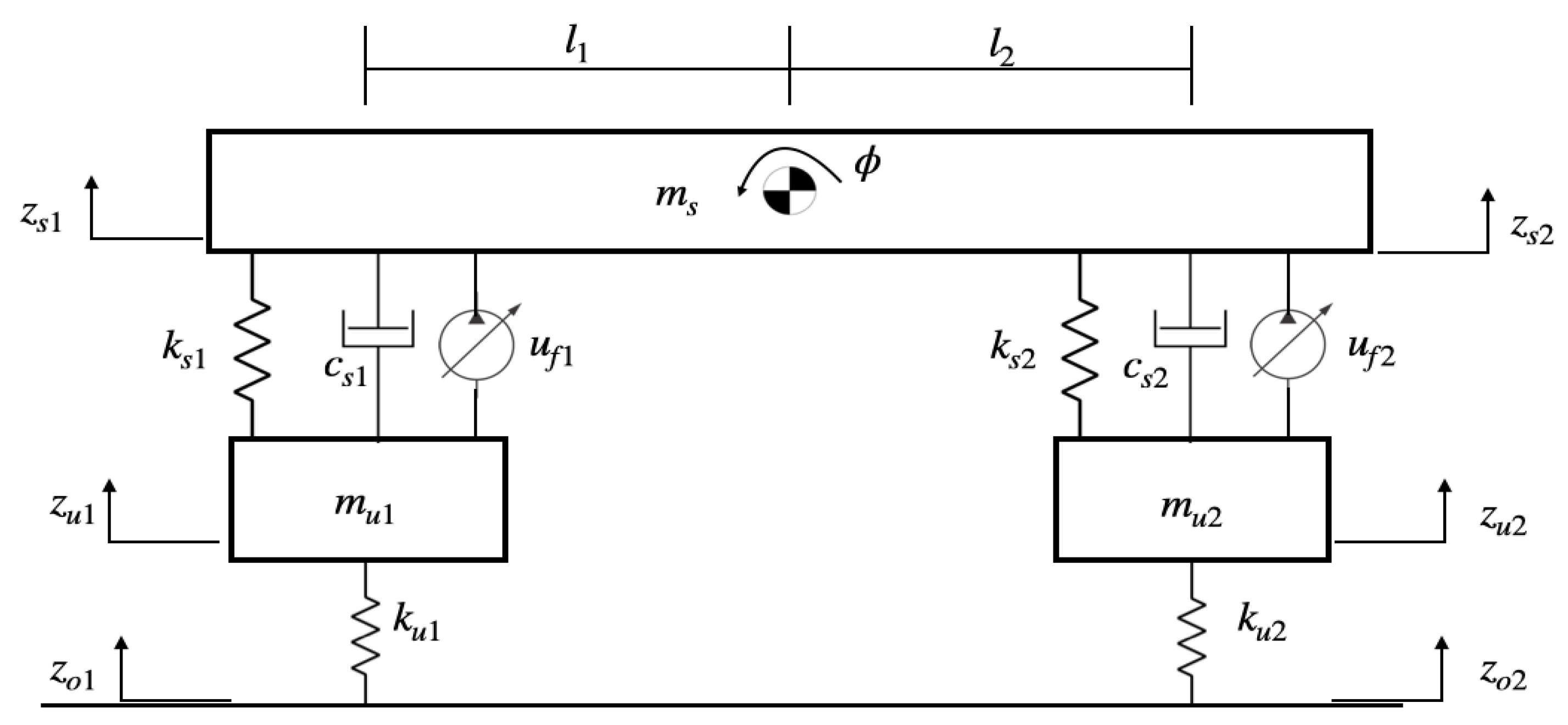
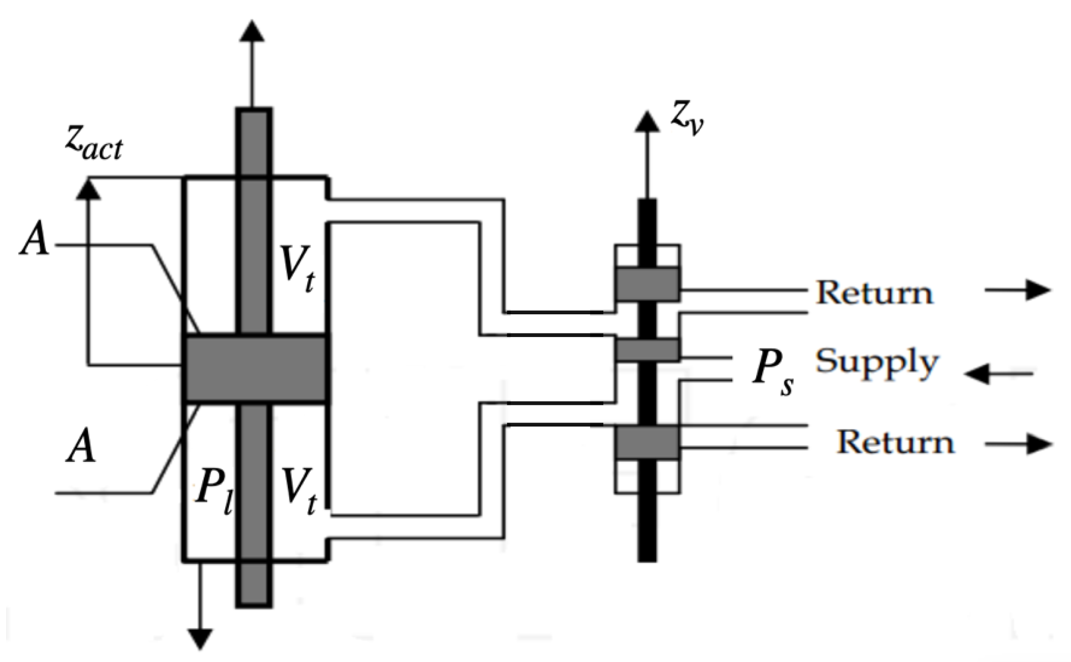
2. Half-Car Active Suspension Model with Electro-Hydraulic Actuators
3. LPV-SS Representation of the Half-Car Active Suspension Model with Fictional Input
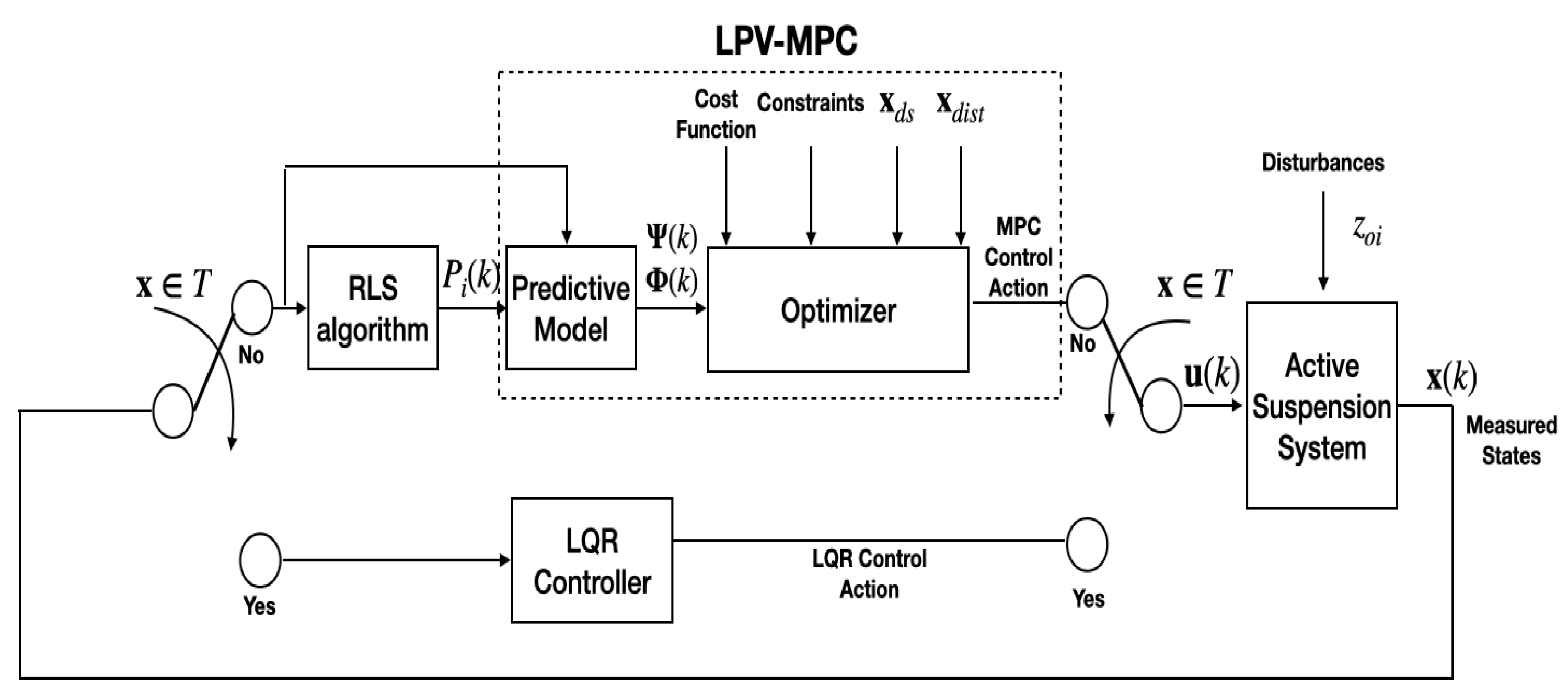
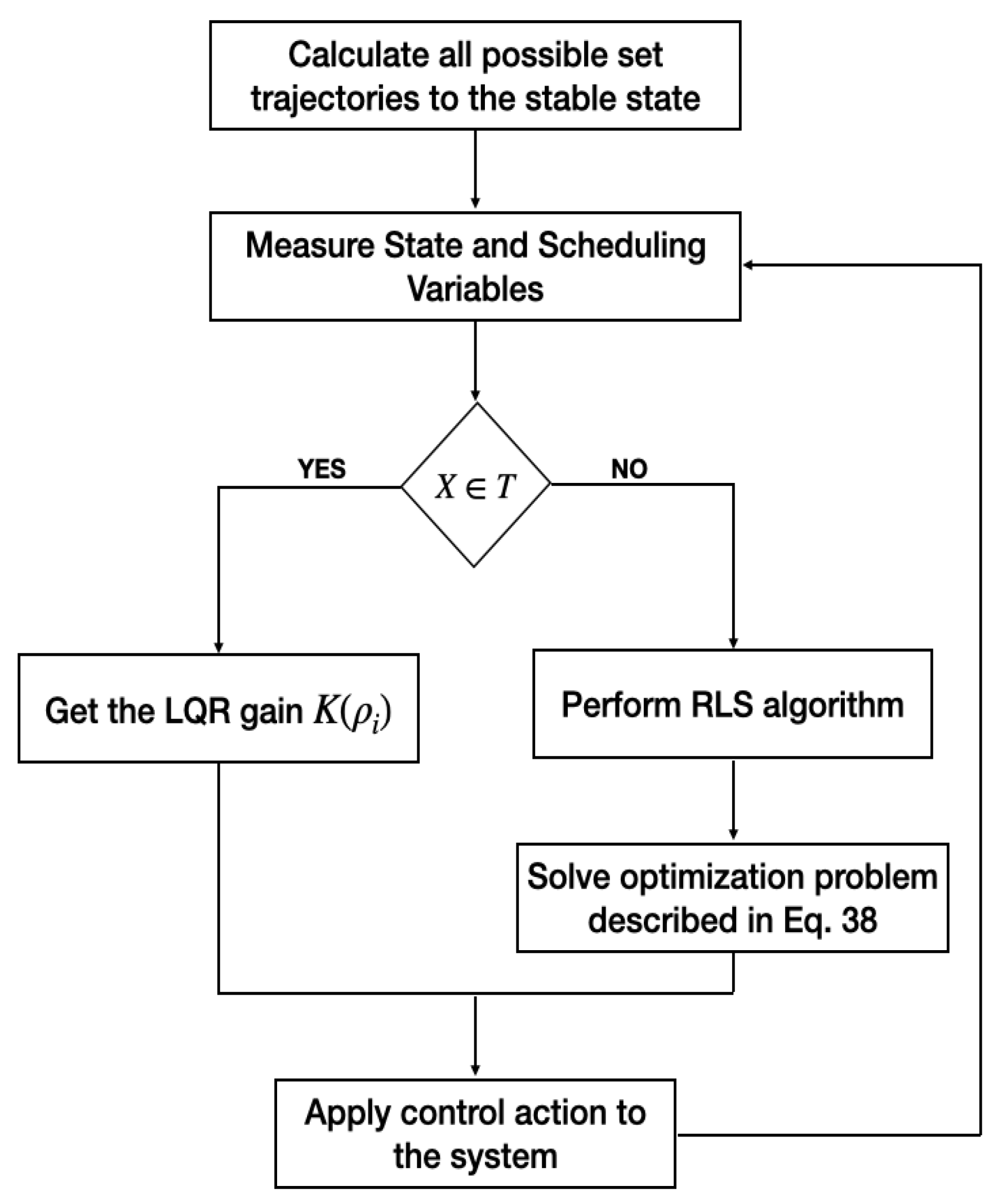
4. LPV-MPC Controller
5. Scheduling Parameters Prediction Using RLS
| Algorithm 1 Recursive Least Squares Algorithm for scheduling parameter prediction |
Offline Step 1—Initialize and Online Step 2—Obtain , and Step 3—Construct vector Step 4—Calculate scalar Step 5—Obtain vector Step 6—Obtain Step 7—Obtain Step 8—Calculate Step 9—Set , If go to Step 10, else, go back to step 3 Step 10—Construct |
6. Quadratic Stability in the LPV-MPC Approach
7. MPC-LQR for LPV Models
7.1. Attraction Sets and Terminal Set
7.2. MPC-LQR Dual Controller
8. Results and Discussion
9. Conclusions and Future Work
Author Contributions
Funding
Institutional Review Board Statement
Informed Consent Statement
Data Availability Statement
Acknowledgments
Conflicts of Interest
References
- Sam, Y.M.; Hudha, K. Modelling and Force Tracking Control of Hydraulic Actuator for an Active Suspension System. In Proceedings of the 1ST IEEE Conference on Industrial Electronics and Applications (2006), Singapore, 24–26 May 2006; pp. 1–6. [Google Scholar] [CrossRef] [Green Version]
- Su, X. Master–slave control for active suspension systems with hydraulic actuator dynamics. IEEE Access 2017, 5, 3612–3621. [Google Scholar] [CrossRef]
- Xiao, L.; Zhu, Y. Sliding-mode output feedback control for active suspension with nonlinear actuator dynamics. J. Vib. Control 2015, 21, 2721–2738. [Google Scholar] [CrossRef]
- Al Aela, A.M.; Kenne, J.-P.; Angue Mintsa, H. A Novel Adaptive and Nonlinear Electrohydraulic Active Suspension Control System with Zero Dynamic Tire Liftoff. Machines 2020, 8, 38. [Google Scholar] [CrossRef]
- Bello, M.M.; Babawuro, A.Y.; Fatai, S. Active suspension force control with electro-hydraulic actuator dynamics. ARPN J. Eng. Appl. Sci. 2015, 10, 17327–17331. [Google Scholar]
- Senthil Kumar, P.; Sivakumar, K.; Kanagarajan, R.; Kuberan, S. Adaptive Neuro Fuzzy Inference System control of active suspension system with actuator dynamics. J. Vibroeng. 2018, 20, 541–549. [Google Scholar] [CrossRef] [Green Version]
- Sam, Y.M.; Suaib, N.M.; Osman, J.H.S. Proportional integral sliding mode control for the half-car active suspension system with hydraulic actuator. In Proceedings of the WSEAS International Conference. In Proceedings of the Mathematics and Computers in Science and Engineering, World Scientific and Engineering Academy and Society, Hangzhou, China, 6–8 April 2018. [Google Scholar]
- Aldair, A.A.; Wang, W.J. Neural controller based full vehicle nonlinear active suspension systems with hydraulic actuators. Int. J. Control Autom. 2011, 4, 79–94. [Google Scholar]
- Aldair, A.A.; Wang, W. FPGA based adaptive neuro fuzzy inference controller for full vehicle nonlinear active suspension systems. Int. J. Artif. Intell. Appl. 2010, 1, 1–15. [Google Scholar] [CrossRef] [Green Version]
- Aldair, A.A.; Wang, W.J. Design of fractional order controller based on evolutionary algorithm for a full vehicle nonlinear active suspension systems. Int. J. Control Autom. 2010, 3, 33–46. [Google Scholar]
- Talib, M.H.A.; Darns, I.Z.M. Self-tuning PID controller for active suspension system with hydraulic actuator. In Proceedings of the 2013 IEEE Symposium on Computers & Informatics (ISCI), Langkawi, Malaysia, 7–9 April 2013; pp. 86–91. [Google Scholar] [CrossRef]
- Ahmed, A.E.N.S.; Ali, A.S.; Ghazaly, N.M.; Abdel-Jaber, G.T. PID controller of active suspension system for a quarter car model. Int. J. Adv. Eng. Technol. 2015, 8, 899–909. [Google Scholar]
- Emam, A.S. Fuzzy Self Tuning of PID controller for active suspension system. Adv. Powertrains Automot. 2015, 1, 34–41. [Google Scholar] [CrossRef]
- Chen, H.; Liu, Z.Y.; Sun, P.Y. Application of constrained H∞ control to active suspension systems on Half-Car models. J. Dyn. Syst. Meas. Control 2005, 127, 345–354. [Google Scholar] [CrossRef]
- Wang, R.; Jing, H.; Karimi, H.R.; Chen, N. Robust fault-tolerant H∞ control of active suspension systems with finite-frequency constraint. Mech. Syst. Signal Process. 2015, 62, 341–355. [Google Scholar] [CrossRef]
- Xu, F.X.; Liu, X.H.; Chen, W.; Zhou, C.; Cao, B.W. Improving handling stability performance of four-wheel steering vehicle based on the H2/H∞ robust control. Appl. Sci. 2019, 9, 857. [Google Scholar] [CrossRef] [Green Version]
- Riofrio, A.; Sanz, S.; Boada, M.J.L.; Boada, B.L. A LQR-based controller with estimation of road bank for improving vehicle lateral and rollover stability via active suspension. Sensors 2017, 17, 2318. [Google Scholar] [CrossRef] [PubMed] [Green Version]
- Yao, Y. Optimization design of active suspension of vehicle based on LQR control. J. Phys.: Conf. Ser. 2020, 1629, 012094. [Google Scholar] [CrossRef]
- Khan, M.A.; Abid, M.; Ahmed, N.; Wadood, A.; Park, H. Nonlinear Control Design of a Half-Car Model Using Feedback Linearization and an LQR Controller. Appl. Sci. 2020, 10, 3075. [Google Scholar] [CrossRef]
- Samadi, F.; Moghadam-Fard, H. Active suspension system control using adaptive neuro fuzzy (anfis) controller. Int. J. Eng. 2015, 28, 396–401. [Google Scholar]
- Zare, K.; Mardani, M.M.; Vafam, N.; Khooban, M.H.; Sadr, S.S.; Dragičević, T. Fuzzy-logic-based adaptive proportional-integral sliding mode control for active suspension vehicle systems: Kalman filtering approach. Inf. Technol. Control 2019, 48, 648–659. [Google Scholar] [CrossRef]
- Zhang, J.; Yang, Y.; Hu, M.; Fu, C.; Zhai, J. Model Predictive Control of Active Suspension for an Electric Vehicle Considering Influence of Braking Intensity. Appl. Sci. 2021, 11, 52. [Google Scholar] [CrossRef]
- Göhrle, C.; Schindler, A.; Wagner, A.; Sawodny, O. Model predictive control of semi-active and active suspension systems with available road preview. In Proceedings of the 2013 European Control Conference (ECC), Zurich, Switzerland, 17–19 July 2013; pp. 1499–1504. [Google Scholar] [CrossRef]
- Theunissen, J.; Sorniotti, A.; Gruber, P.; Fallah, S.; Ricco, M.; Kvasnica, M.; Dhaens, M. Regionless explicit model predictive control of active suspension systems with preview. IEEE Trans. Ind. Electron. 2020, 67, 4877–4888. [Google Scholar] [CrossRef]
- Yao, J.; Wang, M.; Li, Z.; Jia, Y. Research on model predictive control for automobile active tilt based on active suspension. Energies 2021, 14, 671. [Google Scholar] [CrossRef]
- Enders, E.; Burkhard, G.; Munzinger, N. Analysis of the Influence of Suspension Actuator Limitations on Ride Comfort in Passenger Cars Using Model Predictive Control. Actuators 2020, 9, 77. [Google Scholar] [CrossRef]
- Wang, D.; Zhao, D.; Gong, M.; Yang, B. Research on robust model predictive control for electro-hydraulic servo active suspension systems. IEEE Access 2017, 6, 3231–3240. [Google Scholar] [CrossRef]
- Rodriguez-Guevara, D.; Favela-Contreras, A.; Beltran-Carbajal, F.; Sotelo, D.; Sotelo, C. Active Suspension Control Using an MPC-LQR-LPV Controller with Attraction Sets and Quadratic Stability Conditions. Mathematics 2021, 9, 2533. [Google Scholar] [CrossRef]
- Haemers, M.; Derammelaere, S.; Ionescu, C.M.; Stockman, K.; De Viaene, J.; Verbelen, F. Proportional-integral state-feedback controller optimization for a full-car active suspension setup using a genetic algorithm. IFAC-PapersOnLine 2018, 51, 1–6. [Google Scholar] [CrossRef]
- Gustafsson, A.; Sjögren, A. Neural Network Controller for Semi-Active Suspension Systems with Road Preview. Master’s Thesis, Charmers University of Technology, Gothenburg, Sweden, 2019. [Google Scholar]
- Ayub, A.; Sabir, Z.; Shah, S.Z.H.; Wahab, H.A.; Sadat, R.; Ali, M.R. Effects of homogeneous-heterogeneous and Lorentz forces on 3-D radiative magnetized cross nanofluid using two rotating disks. Int. Commun. Heat Mass Transf. 2022, 130, 105778. [Google Scholar] [CrossRef]
- Sadat, R.; Agarwal, P.; Saleh, R.; Ali, M.R. Lie symmetry analysis and invariant solutions of 3D Euler equations for axisymmetric, incompressible, and inviscid flow in the cylindrical coordinates. Adv. Differ. Equ. 2021, 486. [Google Scholar] [CrossRef]
- Ali, M.R.; Ma, W.X.; Sadat, R. Lie symmetry analysis and invariant solutions for (2 + 1) dimensional Bogoyavlensky-Konopelchenko equation with variable-coefficient in wave propagation. J. Ocean. Eng. Sci. 2021. [Google Scholar] [CrossRef]
- Sabir, Z.; Ali, M.R.; Raja, M.A.Z.; Shoaib, M.; Artidoro, R.; Nunez, S.; Sadat, R. Computational intelligence approach using Levenberg—Marquardt backpropagation neural networks to solve the fourth-order nonlinear system of Emden–Fowler model. Eng. Comput. 2021. [Google Scholar] [CrossRef]
- Boyd, S.; Balakrishnan, V.; Feron, E.; ElGhaoui, L. Control system analysis and synthesis via linear matrix inequalities. In Proceedings of the American Control Conference, San Francisco, CA, USA, 2–4 June 1993; pp. 2147–2154. [Google Scholar] [CrossRef] [Green Version]
- Szaszi, I.; Gáspár, P.; Bokor, J. Nonlinear active suspension modelling using linear parameter varying approach. In Proceedings of the 10th Mediterranean Conference on Control and Automation, Lisbon, Portugal, 9–12 July 2002; pp. 1–10. [Google Scholar]
- Morato, M.M.; Normey-Rico, J.E.; Sename, O. Novel qLPV MPC design with least-squares scheduling prediction. IFAC-PapersOnLine 2019, 52, 158–163. [Google Scholar] [CrossRef]
- Franklin, G.F.; Powell, J.D.; Workman, M.L. Digital Control of Dynamic Systems; Addison-Wesley: Reading, MA, USA, 1988; Volume 3. [Google Scholar]
- Boyd, S.; El Ghaoui, L.; Feron, E.; Balakrishnan, V. Linear Matrix Inequalities in System and Control Theory; Society for Industrial and Applied Mathematics: Philadelphia, PA, USA, 1994; Chapter 5; pp. 61–76. [Google Scholar]
- Bumroongsri, P.; Kheawhom, S. An ellipsoidal off-line model predictive control strategy for linear parameter varying systems with applications in chemical processes. Syst. Control Lett. 2012, 61, 435–442. [Google Scholar] [CrossRef]
- Suzukia, H.; Sugie, T. MPC for LPV systems with bounded parameter variation using ellipsoidal set prediction. In Proceedings of the 2006 American Control Conference, Minneapolis, MN, USA, 14–16 June 2006; p. 6. [Google Scholar] [CrossRef]
- Lofberg, J. Automatic robust convex programming. Optim. Methods Softw. 2012, 27, 115–129. [Google Scholar] [CrossRef] [Green Version]


| Variable | Value | Units |
|---|---|---|
| 690 | kg | |
| 40 | kg | |
| 45 | kg | |
| 1222 | kg m | |
| 18,000 | N/m | |
| 22,000 | N/m | |
| 200,000 | N/m | |
| 200,000 | N/m | |
| 1000 | N/(m/s) | |
| 1000 | N/(m/s) | |
| 1.3 | m | |
| 1.5 | m | |
| 10,342,500 | Pa | |
| 1/30 | s | |
| A | m | |
| 1 | s | |
| N/m | ||
| N/m/kg | ||
| m/V |
| Variable | MPC-LQR-LPV | H2(Chen, 2005) | MPC | LQR | Passive |
|---|---|---|---|---|---|
| Chassis Acceleration (m/s) | 0.1580 | 0.5716 | 0.1677 | 0.2671 | 0.7498 |
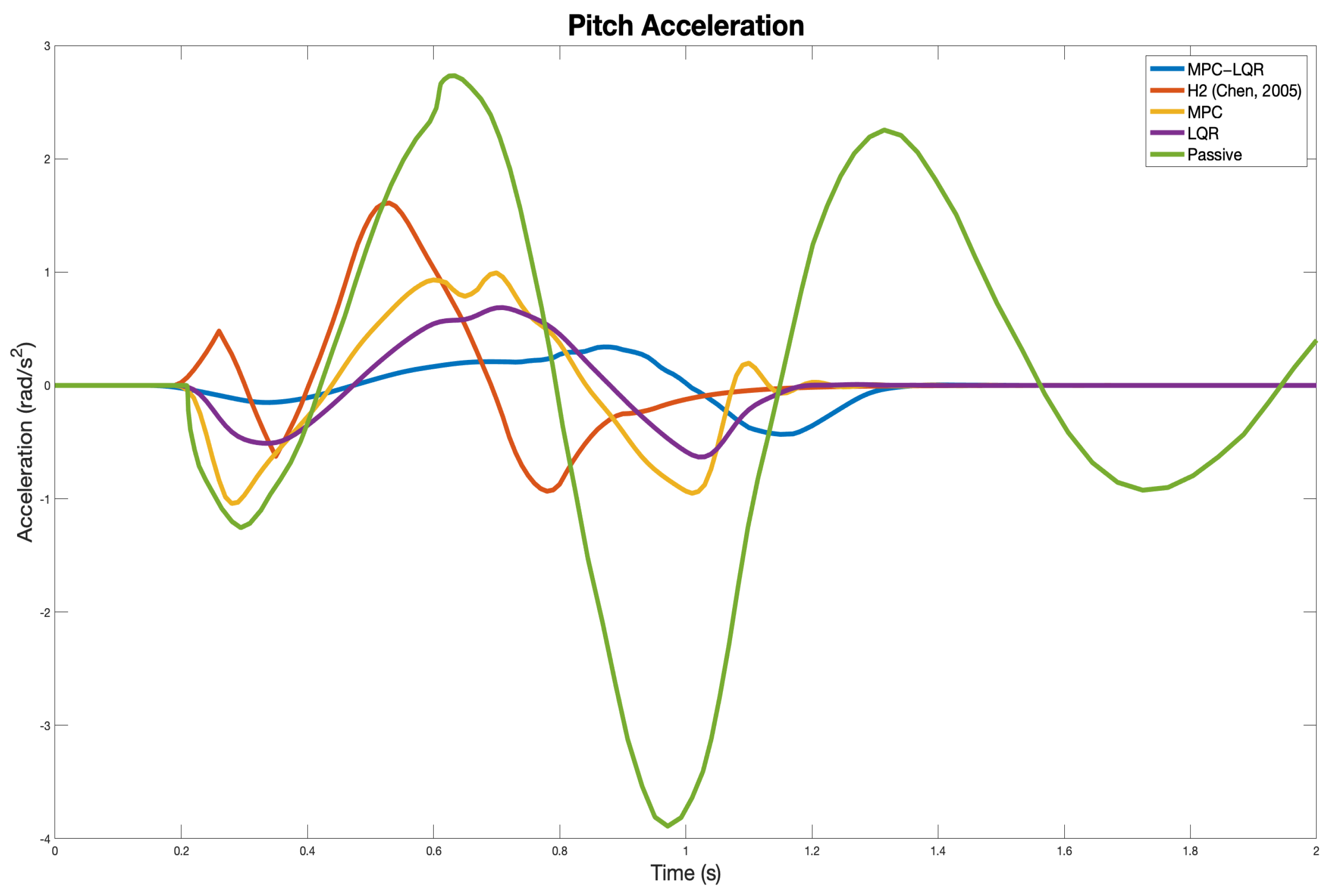
| Pitch Acceleration (rad/s) | 0.1837 | 0.3966 | 0.4349 | 0.2910 | 0.5886 |
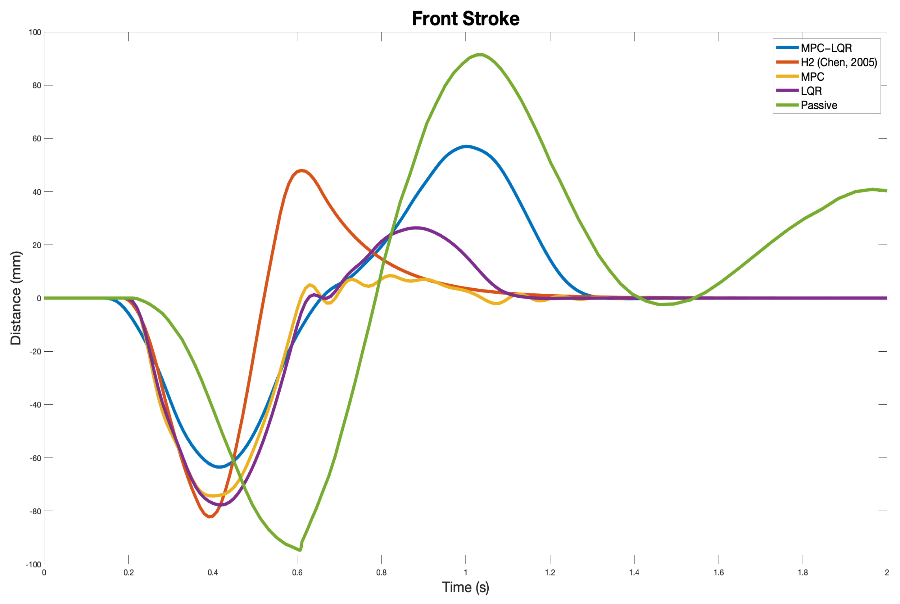
| Front Stroke (m) | 0.0276 | 0.0108 | 0.0238 | 0.0261 | 0.0537 |
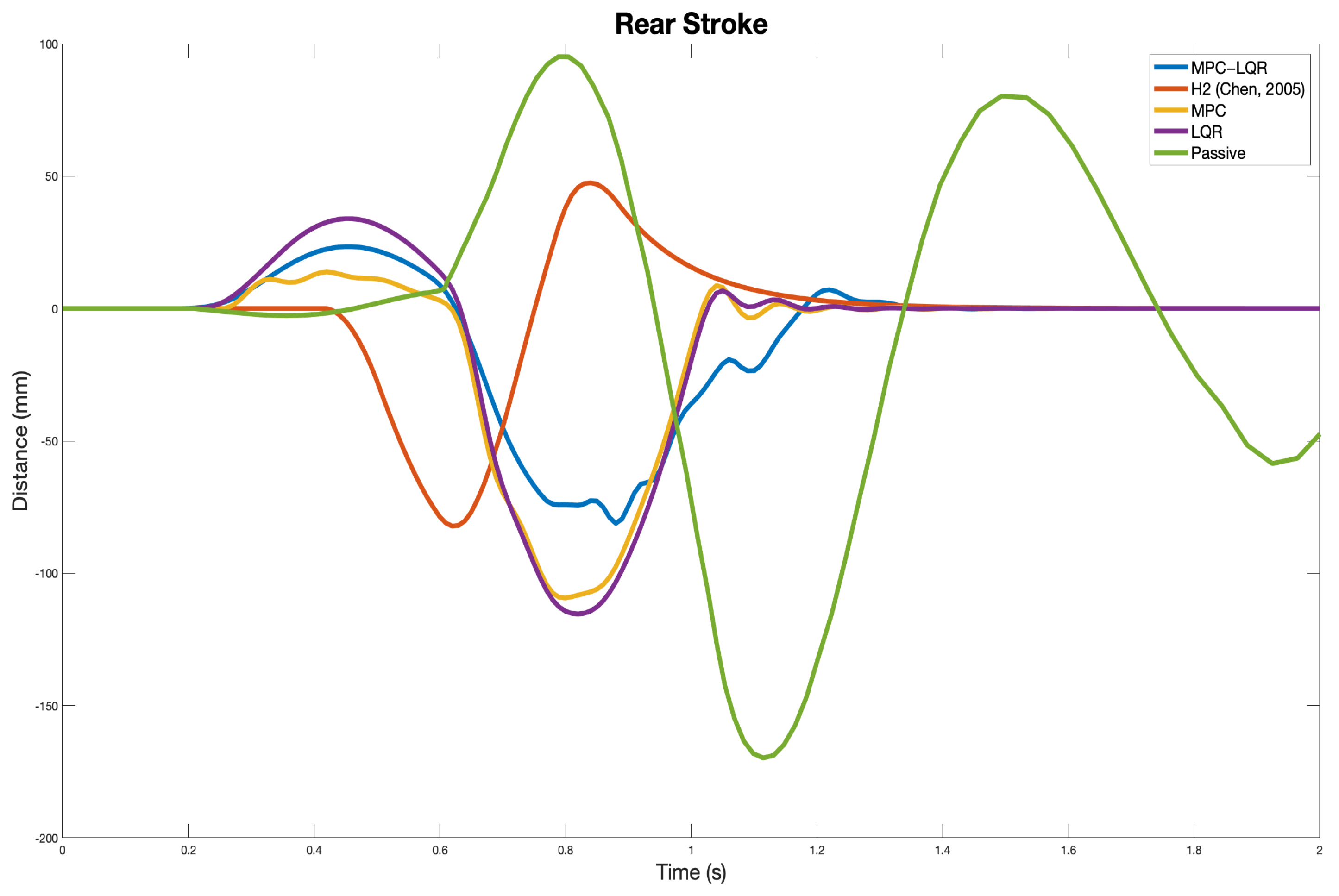
| Rear Stroke (m) | 0.0289 | 0.0102 | 0.0350 | 0.0379 | 0.0665 |
| Variable | MPC-LQR-LPV | H2(Chen, 2005) | MPC | LQR | Passive |
|---|---|---|---|---|---|
| Chassis Acceleration (m/s) | 0.4766 | 1.6402 | 0.5487 | 0.7172 | 3.5120 |
| Pitch Acceleration (rad/s) | 0.5779 | 1.6101 | 1.0416 | 0.6869 | 3.8897 |
| Front Stroke (m) | 0.0635 | 0.0822 | 0.0744 | 0.0777 | 0.0947 |
| Rear Stroke (m) | 0.0814 | 0.0822 | 0.1094 | 0.1154 | 0.1698 |
Publisher’s Note: MDPI stays neutral with regard to jurisdictional claims in published maps and institutional affiliations. |
© 2022 by the authors. Licensee MDPI, Basel, Switzerland. This article is an open access article distributed under the terms and conditions of the Creative Commons Attribution (CC BY) license (https://creativecommons.org/licenses/by/4.0/).
Share and Cite
Rodriguez-Guevara, D.; Favela-Contreras, A.; Beltran-Carbajal, F.; Sotelo, C.; Sotelo, D. An MPC-LQR-LPV Controller with Quadratic Stability Conditions for a Nonlinear Half-Car Active Suspension System with Electro-Hydraulic Actuators. Machines 2022, 10, 137. https://doi.org/10.3390/machines10020137
Rodriguez-Guevara D, Favela-Contreras A, Beltran-Carbajal F, Sotelo C, Sotelo D. An MPC-LQR-LPV Controller with Quadratic Stability Conditions for a Nonlinear Half-Car Active Suspension System with Electro-Hydraulic Actuators. Machines. 2022; 10(2):137. https://doi.org/10.3390/machines10020137
Chicago/Turabian StyleRodriguez-Guevara, Daniel, Antonio Favela-Contreras, Francisco Beltran-Carbajal, Carlos Sotelo, and David Sotelo. 2022. "An MPC-LQR-LPV Controller with Quadratic Stability Conditions for a Nonlinear Half-Car Active Suspension System with Electro-Hydraulic Actuators" Machines 10, no. 2: 137. https://doi.org/10.3390/machines10020137
APA StyleRodriguez-Guevara, D., Favela-Contreras, A., Beltran-Carbajal, F., Sotelo, C., & Sotelo, D. (2022). An MPC-LQR-LPV Controller with Quadratic Stability Conditions for a Nonlinear Half-Car Active Suspension System with Electro-Hydraulic Actuators. Machines, 10(2), 137. https://doi.org/10.3390/machines10020137