Visualized Stacked Denoising Auto-Encoder Model for Extracting and Evaluating the State Features of Rolling Bearings

Abstract

Extracting intuitive operating state features from vibration signals without prior knowledge is a prospective requirement for health monitoring and fault diagnosis in bearings. In this paper, a visualized stacked denoising auto-encoder (VSDAE) model is proposed for the unsupervised extraction and quantitative evaluation of bearings’ state features. First, the stacked denoising auto-encoder (SDAE) was used to reconstruct vibration signals. The intermediate vector of the SDAE, which is a high-information-density representation of vibration signals, was regarded as the pending state feature. Then, the dimension of the intermediate vector was reduced by the t-distributed stochastic neighbor embedding (t-SNE) method to the two-dimensional visualization space. Finally, the silhouette coefficient of feature distribution was calculated to quantitatively evaluate the extracted features. The proposed model was evaluated using experimental bearing signals simulating various operating states. The results proved that the features, extracted and evaluated by the VSDAE, allowed the recognition of the operating states of the examined bearings.

1. Introduction

Rolling bearings are widely used in a variety of electromechanical equipment and play the role of joints between stationary parts and rotating parts in rotating mechanisms. Generally, rolling bearings bear an uninterrupted load under harsh working conditions, which makes them the most easily damaged parts [1,2]. The state of rolling bearings is closely related to the safe and smooth operation of the equipment. Therefore, health monitoring and fault diagnosis of rolling bearings is particularly important for industrial process. Since vibration signals carry adequate information of the operating state of bearings, extracting features from vibration signals becomes the fundamental task of health monitoring and fault diagnosis in bearings.

The purpose of feature extraction is to search failure-induced or performance degradation indicators from the original vibration signals. Moreover, the dimension of the extracted feature should be much smaller than that of the original signals. Many feature extraction methods have been developed in three domains, namely, the time domain, the frequency domain and the time–frequency domain, to pre-process the vibration signals of bearings [3]. For feature extraction in the time domain, statistical analysis and probability density estimation are common tools. Statistical features, such as root mean square, standard deviation and variance, are calculated to discover the phenomenon of amplitude variation caused by bearing failures. Non-dimensional features, such as kurtosis, skewness, shape factor, crest factor, etc., are estimated to quantify the change in probability distribution related to bearing failures [4]. In addition, measures of the chaotic degree of vibration signals, such as entropy and correlation dimension, are also used to judge the health state of bearings [5]. These features, extracted in the time domain, have the lowest dimensionality compared to those extracted in the other domains, but only specific state information rather than overall state information can be represented. When the vibration signals are transformed from the time domain to the frequency domain, the periodic state information is preserved, and the non-periodic noise is suppressed. Therefore, frequency-domain features, such as spectrum kurtosis and failure pass frequency, become the most widely used diagnostic criteria in the industrial field [6,7]. However, the variety of working conditions and the reliance on bearings’ structural parameters are still issues to consider for the application of frequency-domain features. As non-stationary vibration signals have started to receive increasing attention, feature extraction in the time–frequency domain has been developed. Numerous signal decomposition methods, such as wavelet decomposition [8,9], empirical mode decomposition [10], local mean decomposition [11], variational mode decomposition [12], etc., are proposed to separate the time-varying failure components from the vibration signals. Compared with the features extracted in the time domain and frequency domain, the time–frequency-domain features contain the most abundant and accurate state information. However, the disadvantage of these methods is that the decomposition parameters need to be pre-determined empirically. In summary, the above-mentioned feature extraction methods, which provide convenience for bearings’ health monitoring and fault diagnosis, always rely on a prior knowledge of bearing failures that is hard to obtain in practical applications.

With the development of information technology, feature extraction methods have gradually been pushed forward to a new direction of deep learning (DL) [13,14]. Unlike traditional signal processing methods, DL-based models have powerful feature self-learning ability, which can directly extract low-level features from raw data and aggregate them to generate high-information-density features. The convolutional neural networks (CNNs) are among the most effective DL-based models to extract features [15]. During the end-to-end learning process of CNNs, the features of bearing failure are automatically caught and memorized in the multilayer networks’ structures. Many novel network architectures and learning strategies, such as capsule network [16], feature-aligned module [17], block attention module [18], etc., have been combined with CNNs to improve the robustness of the extracted features. Because the rolling bearing cannot be disassembled to examine a potential failure during service, feature extraction has to process vibration signals without prior knowledge. Unsupervised or self-supervised DL methods, represented by the auto-encoder, have become attractive solutions and received increasing research attention.

The auto-encoder, proposed by Rumelhart et al. [19], is a typical single-hidden-layer neural network. It can compress and reconstruct data to accomplish learning without the corresponding label information. The intermediate vector generated by the compressing process is a high-information-density representation of the original data. Therefore, the intermediate vector generated by the auto-encoder that completed training can be regarded as the extracted feature of the input data. Since the interference noise in the training signals may significantly affect the learning results of the auto-encoder, a denoising auto-encoder (DAE) was proposed by Vincent et al. [20]. In the DAE, noise is artificially added to the original data to produce a damaged input, and the corresponding clean input is reconstructed. Although the robustness of the auto-encoder has been greatly improved by the denoising mechanism, the auto-encoder still tends to fall into local optimization during training, which leads to a poor performance of feature extraction. To avoid this disadvantage, a stacked denoising auto-encoder (SDAE) was proposed [21]. In the SDAE, the weights of the deep neural network are initialized in a layer-by-layer unsupervised learning manner, and a small number of labeled samples are used to fine-tune the network. With the help of these improvements, the auto-encoder has been relieved from noise interference and over-fitting learning and has developed into a series of effective feature extraction tools.

Models based on the auto-encoder have been also widely applied in the field of feature extraction of mechanical failures. In [22], the auto-encoder was combined with an extreme learning machine to adaptively mine the discriminative failure features and achieve a rapid diagnosis. Ma et al. combined a stacked auto-encoder with a generative adversarial network and proposed a method for transformer anomaly detection utilizing the vibration signals of the normal operating state [23]. In [24], SDAE were used to extract the features of the vibration signals, and the output features were clustered to identify the different failures of rolling bearings. The results showed that as the number of the hidden layers increased, all the fault samples under different conditions could be better separated using the SDAE compared to other feature extraction models. However, there are still some problems in practical feature extraction using the auto-encoder. The features extracted by the auto-encoder have no specific meaning, which has a negative effect on the direct interpretation of the rolling bearing state information represented by the features. Therefore, it is difficult to determine the thresholds corresponding to different operating states based on these features. Meanwhile, there is no intuitive and reliable way to evaluate the performance of the extracted features for state identification. In this situation, the models based on the auto-encoder have to combined with other intelligent algorithms to improve the intuitiveness and evaluability of the extraction results.

In this paper, a visualized stacked denoised auto-encoder model (VSDAE) is proposed to extract and evaluate the operating state features of rolling bearings. By the multiple encoder layers and noise reduction mechanism of the SDAE, the features contained in the vibration signals were learned so to improve the generalization ability and suppress the over-fitting. Then, t-distributed stochastic neighbor embedding (t-SNE) was integrated to transform the features extracted by the SDAE into two-dimensional distributions. Finally, referring to human visual attention mechanism, the silhouette coefficient of two-dimensional distribution was introduced to quantitatively evaluate the extracted features. The contributions of this paper can be mainly summarized as follows: (1) The operating state features of rolling bearings were extracted in an unsupervised manner by the SDAE; (2) A visual presentation of the features extracted from the vibration signals was provided to evaluate the ability of state recognition.

The remainder of the paper is organized as follows. The fundamentals and methodologies of the VSDAE are described in Section 2. Section 3 shows the experimental verification on a bearing failure simulation bench. Finally, the conclusions are presented in Section 4.

2. Visualized Stacked Denoised Auto-Encoder

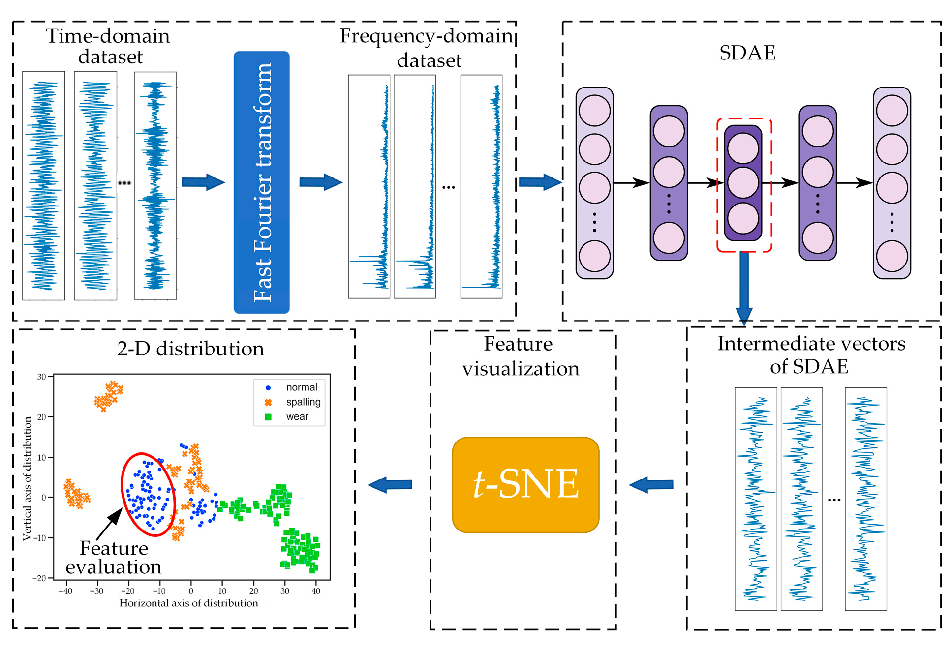
The VSDAE model consists of three sequential stages: feature extraction, feature visualization and feature evaluation. The feature extraction is executed by the SDAE. In this stage, vibration signals collected in various operating states are directly used to construct input datasets, including a time-domain dataset and a frequency-domain dataset, for learning. The intermediate feature vectors of the encoder are obtained after the learning process through compression and reconstruction. In the feature visualization stage, the dimension of the feature vectors is reduced by t-SNE, and a two-dimensional distribution graph is generated. By this means, the differences between high-dimensional features can be displayed in the two-dimensional graph. In the feature evaluation stage, the visual attention mechanism is utilized as a reference, and the silhouette coefficients of all features are calculated and averaged to evaluate the ability of the extracted features to identify operating states. In this stage, the way that a human pays attention to the information contained in the distribution graph is imitated, so the effect of the extracted features can be intuitively and accurately evaluated. The flowchart of the VSDAE is shown in Figure 1, and the detailed procedures are described below.

2.1. Feature Extraction Utilizing the SDAE

The SDAE was developed on the basis of the auto-encoder and has been improved according to the defects of auto-encoder. For the original auto-encoder, the training process is executed by an encoder and a decoder. In the encoder, the given one-dimensional sequence $F$ is input, and the intermediate vector $H$, in which $F$ is encoded, is calculated as:

$$H=f\left(W_{enc}F+b_{enc}\right),$$

(1)

where $f\left(·\right)$ is the nonlinear activation function; $W_{enc}$ and $b_{enc}$ are the internal weight matrix and offset matrix of the encoder, respectively. Then, $H$ is input to the decoder, and $F$ is reconstructed as:

$$\tilde{F}=f\left(W_{dec}H+b_{dec}\right),$$

(2)

where $W_{enc}$ and $b_{enc}$ are the internal weight matrix and offset matrix of the encoder, respectively. The model is trained by the back-propagation algorithm, and the reconstruction error between $F$ and $\tilde{F}$ is iteratively optimized to drop to a predetermined range. The optimization problem can be described as:

$$\underset{\theta }{\min }L\left(\theta \right)={\Vert \tilde{F}-F\Vert }_2^2; \theta =\left[W_{enc},b_{enc},W_{dec},b_{dec}\right].$$

(3)

The noise reduction mechanism is added in the training of the auto-encoder to form the DAE. Firstly, a certain percentage of points in $F$ are randomly zeroed to obtain a damaged input sequence $F_d$. Then, $F_d$ is fed into the encoder to obtain the intermediate vector $H_d$ and the reconstruction sequence $\widetilde{F_d}$. 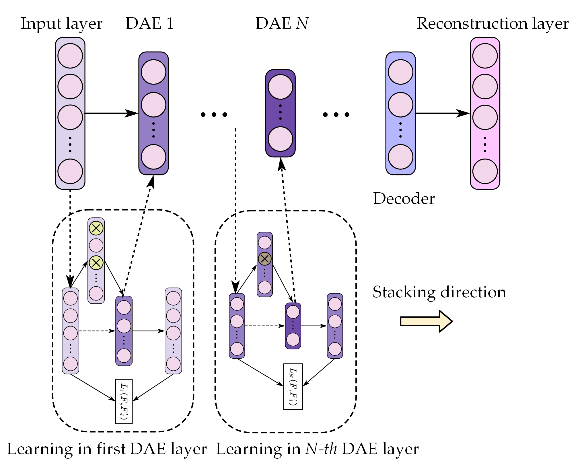The reconstruction error $L\left(F,\widetilde{F_d}\right)$ between input sequence $F$ and reconstruction sequence $\widetilde{F_d}$ is minimized in the encoder, which is trained by the back-propagation algorithm. With the help of the introduction of a corrupted input, the robustness of the auto-encoder is improved. The architecture of the DAE is shown in Figure 2.

By stacking the DAEs layer by layer, a deep learning network, called stacked denoising auto-encoder (SDAE), can be constructed. It has been verified that the larger the network depth, i.e., the number of layers of the auto-encoder, is, the better the learning performance of the SDAE is. The learning procedure of the SDAE with $N$ layers is as follows:

• Given the initial input, the first DAE is trained in an unsupervised manner to reduce the reconstruction error to the predetermined value.
• Take the output of the hidden layer of the current DAE as the input of the next DAE and train the DAE in the same way.
• Repeat the second step until all DAEs have been trained.

After the SDAE completes the learning procedure shown in Figure 3, the weights of the encoder retain the mapping rules for feature extraction. Since the intermediate vector in the N-th DAE layer, denoted as $H_d^N$, is directly connected to the subsequent decoders, it is regarded as a centralized information representation of the original input. In the VSDAE model, $H_d^N$ is used as the feature extracted by the SDAE.

2.2. Feature Visualization Utilizing t-SNE

If $H_d^N$ is a $l$-dimensional vector where $l>3$, it cannot be directly observed. However, the practical dimension of the intermediate vector is always larger than the dimension of visualization. Therefore, in the proposed model, t-SNE [25] was used to further reduce the dimension of the feature vector, and a two-dimensional distribution graph was generated to represent the feature information in a visual way. In t-SNE, the analysis of the sample distribution is converted into the analysis of the probability distribution. Although the sample distributions before and after dimensionality reduction are significantly different, their probability distribution will be close enough after the space embedding operation of t-SNE.

Suppose the original distribution of $H_d^N$ is $\left(h_1,h_2,\cdots ,h_n\right)$, where $h_i$ represents a point in the $l$-dimensional space, and the distribution after dimensionality reduction is $\left(z_1,z_2,\cdots ,z_n\right)$, where $z_i$ represents a point in the two-dimensional space; their probability distributions are defined as:

$$P\left(j|i\right)=\frac{S\left(h_i,h_j\right)}{{{\displaystyle \sum }}_{k\ne i}S\left(h_i,h_k\right)}, j\ne i, i=1,2,\dots n$$

(4)

$$Q\left(j|i\right)=\frac{S^{\prime }\left(z_i,z_j\right)}{{{\displaystyle \sum }}_{k\ne i}{S}^{\prime }\left(z_i,z_k\right)},j\ne i,i=1,2,\dots n$$

(5)

where $P\left(j|i\right)$ and $Q\left(j|i\right)$ are the probability distributions before and after dimensionality reduction; $S\left(·\right)$ and $S^{\prime }\left(·\right),$ respectively, represent the similarity measure function, i.e.:

$$S\left(h_i,h_j\right)=\exp \left(-{\Vert h_i-h_j\Vert }_2^2\right)$$

(6)

$$S^{\prime }\left(z_i,z_j\right)={\left[1+{\Vert z_i-z_j\Vert }_2^2\right]}^{-1}$$

(7)

A loss function is defined to calculate the difference between the two probability distributions:

$$L\left(z_1,z_2,\dots , z_n\right)={{\displaystyle \sum }}_{i=1}^n{D}_{KL}(P(j|i)\left|\right|Q\left(j|i\right))={{\displaystyle \sum }}_{i=1}^n{{\displaystyle \sum }}_{j\ne i}P\left(j|i\right)\log \left(\frac{P(j|i)}{Q(j|i)}\right),$$

(8)

where $D_{KL}$ denotes the Kullback–Leibler divergence. Since the dimensionality reduction problem is equivalent to the minimizing difference between two probability distributions, the gradient descent algorithm is used to solve the smallest value of $L\left(z_1,z_2,\dots , z_n\right).$ The solution procedure is presented in Equations (9)–(11).

$$\frac{\partial L}{\partial Z^{\left(0\right)}}={\left(\frac{\partial L}{\partial z_1^{\left(0\right)}},\frac{\partial L}{\partial z_2^{\left(0\right)}},\dots ,\frac{\partial L}{\partial z_n^{\left(0\right)}}\right)}^T$$

(9)

$$Z^{\left(1\right)}=Z^{\left(0\right)}+\eta \frac{\partial L}{\partial Z^{\left(0\right)}}$$

(10)

$$\left(z_1^{*},z_2^{*},\dots ,z_n^{*}\right)=\underset{{\mathrm{z}}_1,{\mathrm{z}}_2,\dots ,{\mathrm{z}}_n}{\mathrm{argmin}}L\left(z_1,z_2,\dots ,z_n\right),$$

(11)

where $\eta$ is the learning rate, and $\left(z_1^{*},z_2^{*},\dots ,z_n^{*}\right)$ are the solved distribution points in the target dimension. After the above operations, the features extracted by the SDAE are embedded in the two-dimensional space and realized visualization.

2.3. Feature Evaluation

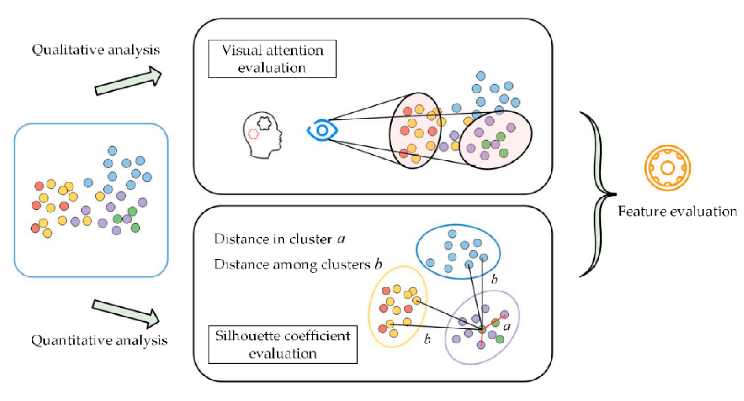
To evaluate the ability of the features in the form of a two-dimensional distribution to distinguish the operation states of rolling bearings, referring to the qualitative visual attention evaluation, a silhouette coefficient is used to achieve a quantitative evaluation of the extracted features. The schematic diagram of feature evaluation is illustrated in Figure 4. If the two-dimensional distribution points are marked with different colors according to the represented operating states, visual attention can easily be used to determine the corresponding state depending on visual factors such as the distribution position of the points, the color of the points, the distance of a point from other points, etc. The boundaries of different distribution clusters are the main criteria for judgment. Therefore, the silhouette coefficient in the cluster analysis is used as the quantitative analysis indicator.

When the features are embedded in the two-dimensional space, the distribution points corresponding to the same operating state are expected to be clustered in a compact cluster. Meanwhile, the distribution points corresponding to other operating states should be far away from this cluster. The silhouette coefficient of feature distribution clusters quantifies the degree of the above expectations.

For a distribution cluster corresponding to the operating state $S_i$, the average distance from a distribution point $i$ to other distribution points in $S_i$ is denoted as $a\left(i\right)$, and the minimum average distance from the distribution point $i$ to other distribution clusters is denoted as $b\left(i\right)$. The two distance parameters, $a\left(i\right)$ and $b\left(i\right)$, are calculated as follows:

$$a\left(i\right)=\frac{{{\displaystyle \sum }}_{k\in S_i,i\ne k}dist\left(i,k\right)}{n_i-1}$$

(12)

$$b\left(i\right)=\underset{S_j,1\le j\le k,j\ne i}{\min }\left\{\frac{{{\displaystyle \sum }}_{t\in S_j}dist\left(i,t\right)}{n_{j }}\right\},$$

(13)

where $n_i$ is the number of distribution points corresponding to $S_i$, $dist\left( ,\right)$ represents the calculation of the Euclidean distance, and $k$ is the number of operating states. The silhouette coefficient of the distribution point $i$ is defined as:

$$S\left(i\right)=\frac{b\left(i\right)-a\left(i\right)}{\max \left\{a\left(i\right),b\left(i\right)\right\}}$$

(14)

The overall silhouette coefficient of all distribution points $S$ can be specified as the average of all $S\left(i\right)$. Obviously, the value of $S$ is between −1 and 1. The closer $S$ is to 1, the higher the degree of aggregation within the state clusters, and the farther the separation among the clusters. In this situation, the extracted features are expected to identify the operating states.

By integrating the above feature extraction, feature visualization and feature evaluation, the VSDAE model was constructed. Vibration signals were abstracted as high-dimensional intermediate features, which were embedded into the two-dimensional distribution space and finally evaluated using the silhouette coefficient. Compared with the SDAE, the advantage of the proposed VSDAE is that it can display features in a visual graph and intuitively determine the boundaries of different operating states. Although it requires some additional calculation, it is acceptable in most applications.

3. Experimental Verification

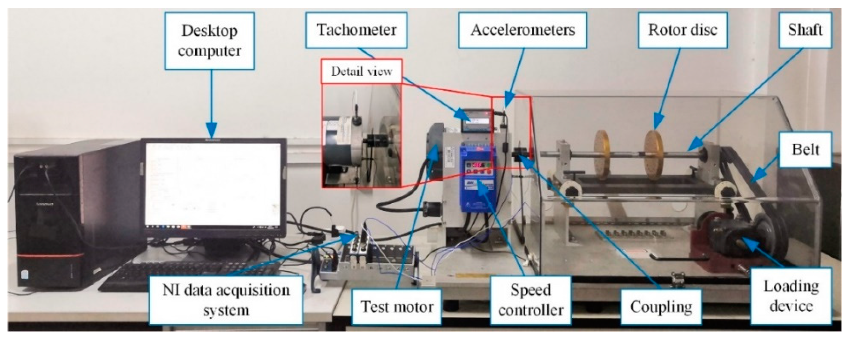
A motor bearing failure bench, whose setup is shown in Figure 5, was used to supply the experimental vibration signals. Defective test bearings, model 6203-2RS, were installed in the motor to simulate the different bearing operating states in industrial applications. Due to the closed structure of the motor, a radial load could not be directly applied to the test bearings. Therefore, a magnetic clutch was used to generate the torque load, which varied from 0.5 to 10 in-lbs and corresponded to six adjustment levels. The speed of the motor was adjusted using a speed controller. An acceleration sensor, PCB PIEZOTRONICS 352C68, was installed on the motor shell at the end of the drive to collect the vibration signals. The installation direction was the horizontal radial direction. The sampling frequency was set at 12,800 Hz, and the sampling length was set at 15 s.

Three typical bearing operating states, i.e., normal, spalling and wear, were simulated in the experiment. Thereinto, the experiment in the normal state was executed with four different sound bearings. The failure of spalling, shown in Figure 6a, was made by laser sintering. Four sintering sizes of 0.8 mm, 1.0 mm, 1.2 mm and 1.4 mm were used to simulate the gradual expansion of the spalling area. Moreover, different wear areas were grinded on the outer raceway to simulate the wear failure. The wear areas occupied 1/8, 1/4, 1/3 and 1/2 of the outer raceway, respectively. One of the simulated wear failures is shown in Figure 6b. In this way, a total of 12 simulated operating states were generated. In each simulated state, six levels of torque loads were applied to the rotor and transferred to the bearings. Five sets of vibration signals were collected under each simulated state and applied load. Among the above five sets of vibration signals, four sets of signals were randomly selected as the learning sample, and the remaining one was used for testing. That is to say, there were a total of 288 datasets to be learned.

Considering that the VSDAE is an end-to-end unsupervised learning model, the additional pre-processing was omitted. The data fragments of length 1024 were randomly truncated from each set of vibration signal as the time-domain dataset. In addition, another signal segment of length 2048 was truncated, and its spectrum was calculated by the fast Fourier transformation. The time-domain data and the frequency-domain data under different operating states ware shown in Figure 7. For the original vibration signal in the time domain, the random noise was uniformly distributed over all sampling moments. When the vibration signals were transformed into frequency-domain signals by FFT, the random noise without periodicity was suppressed. The residual noise was non-uniformly distributed in the spectrum. Since the meaningful data points in the spectrum were 1024, the first 1024 spectrum amplitudes were set as the frequency-domain dataset. In this way, the lengths of the time-domain dataset and frequency-domain dataset were the same. To avoid the influence of different values on the learning effect, all datasets were normalized.

The time-domain dataset and the frequency-domain dataset were learned by the proposed VSDAE model. The parameters of the VSDAE model are shown in

Table 1. Structural parameters of the VSDAE for the time-domain dataset.

No.	Parameter Name	Parameter Value
1	Numbers of nodes in each layer of the encoder	1024-2000-2500
2	Number of nodes in the intermediate layer	300
3	Numbers of nodes in each layer of the decoder	2500-2000-1024
4	Damage proportion of the input sequence	10%
5	Damage proportion of the overall sequence	10%
6	Optimizer	Stochastic gradient descent
7	Learning rate	0.1

and

Table 2. Structural parameters of the VSADE for the frequency-domain dataset.

No.	Parameter Name	Parameter Value
1	Numbers of nodes in each layer of the encoder	1024-1500-2000
2	Number of nodes in the intermediate layer	200
3	Numbers of nodes in each layer of the decoder	2000-1500-1024
4	Damage proportion of the input sequence	10%
5	Damage proportion of the overall sequence	10%
6	Optimizer	Stochastic gradient descent
7	Learning rate	0.1

. The number of stacked DAE layers was set to 3. To achieve noise reduction in the auto-encoder, the damage proportions of input sequence and over sequence were set to 10%. The learning rate is a parameter that directly affects the efficiency, quality and convergence of network learning. To ensure the convergence of our model, it was set to 0.1.

The rounds of overall training were 200. For comparison, a popular method for dimensionality reduction and feature extraction, called kernel principal component analysis (KPCA) [26], was also used to deal with the datasets. For the KPCA, the target dimension was set to 300, and the radial basis function was selected as the kernel function.

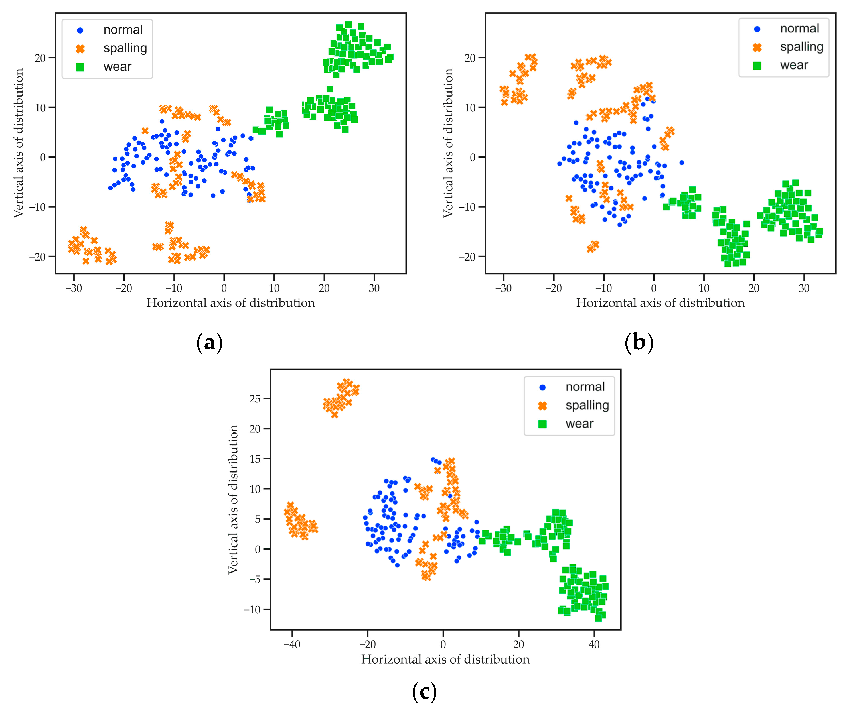
Firstly, the time-domain dataset was input in the SDAE to extract the features. After the learning process, the intermediate vectors were embedded in the two-dimensional space by t-SNE. The obtained distribution graph is shown in Figure 8c. To analyze the feature extraction ability of the SDAE, the original time-domain dataset was also reduced to a two-dimensional space by t-SNE; its distribution graph is shown in Figure 8a. The feature vectors extracted by KPCA were embedded into the same visible distribution space by t-SNE, and the result are shown in Figure 8b. In these distribution graphs, the blue dots correspond to the normal state, the yellow forks correspond to the spalling failure state, and the green squares correspond to the wear failure state. It can be seen that the point distribution of different states was chaotic in the absence of feature extraction by the SDAE. Therefore, the visualized distribution of the original time-domain dataset could not be used to identify the operating conditions. The feature distribution, obtained by the KPCA and t-SNE, exhibited certain homogeneous clustering properties, but the mixture of the three states in the central region was unacceptable. On the contrary, the feature distribution obtained by the SDAE and t-SNE, avoided the intersection of the three operating states. However, the distribution points corresponding to normal state and spalling failure still could not be distinguished. It can be concluded that the combination of SDAE and t-SNE provided the best feature distribution. In addition, the noise in the time-domain dataset affected the state distinguishability of all distributions.

Then, the frequency-domain dataset was input in the SDAE to extract the features. We used t-SNE to generate the visualized distribution graphs of the original frequency-domain dataset, the extracted features by the KPCA, and the extracted features by the SDAE. The results are compared in Figure 9a–c. It is obvious that the frequency-domain dataset had a better ability to distinguish different states than the time-domain dataset. The distribution graphs of the extracted feature by both KPCA and the SDAE exhibited a stronger aggregation in the same state than that observed with the original frequency-domain dataset. It is beneficial to distinguish different operating states. By comparing Figure 9b,c, it was observed that the distribution points in Figure 9c presented a better homogeneous clustering property than those shown in Figure 9b. For the intersection of the distribution points corresponding to normal state and spalling failure, Figure 9b displays more mixed areas than Figure 9c. It proves that the SDAE had a better feature extraction performance than KPCA. In addition, the dimension of the extracted features was 200, equal to the number of nodes in the intermediate layer. In contrast, the dimension of the original frequency-domain dataset was 1024, and the dimension of the features extracted by KPCA was 300. The high-information-density representation ability of the SDAE was verified. The above results proved that the operating state information of the bearings was succesfully extracted by the SDAE and visualized by t-SNE.

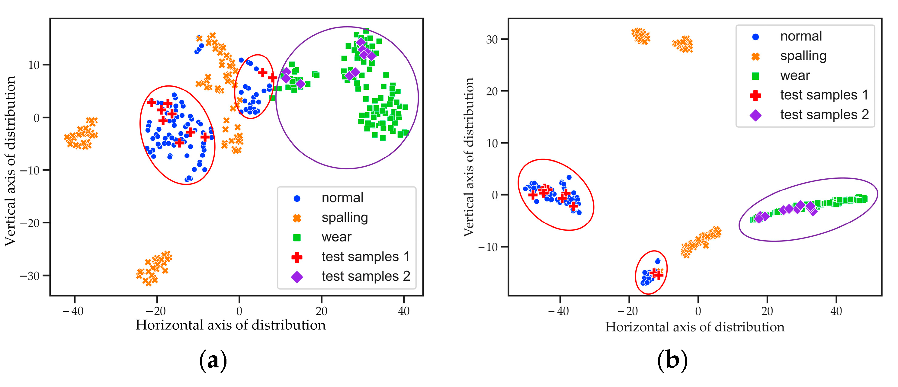
To verify the feature evaluation, a test sample was randomly selected from the testing dataset corresponding to the normal state. The spectrum of the test sample was processed by the SDAE and t-SNE, and the obtained distribution point is displayed in Figure 10. For a comparison with the learning dataset, the test distribution point was portrayed together with the distribution points of the learning dataset and marked with red cross. It can be seen that the distribution point of the test sample fell within the distribution cluster corresponding to the normal state. This distribution result was consistent with the qualitative visual attention evaluation. When the distribution point of the test sample was considered to correspond to an unknown new state, the calculated overall silhouette coefficient $S$ was 0.0534. If the corresponding state of the distribution point of the test sample was assumed to be normal, spalling and wear, $S$ was, respectively, 0.3149, 0.3101 and 0.3071. The maximum of $S$ corresponded exactly to the normal state. The quantitative evaluation of the extracted features was thus verified.

To further verify the performance of feature evaluation, 10 test samples corresponding to the normal state and 10 test samples corresponding to the wear failure were randomly selected from the testing dataset. These test samples together with the learning dataset were processed to extract and visualize their features. The obtained feature distribution is shown in Figure 11a. The distribution points corresponding to the normal state were marked with a red cross, and the distribution points corresponding the wear failure were marked with a purple diamond. All the test samples fell within the distribution clusters corresponding to the normal state. When the distribution points of all the test samples corresponded to the spalling failure, the overall silhouette coefficient $S$ was 0.239. If they corresponded to the wear failure, $S$ was 0.266. When the distribution points of all test samples corresponded to the normal state, the maximum value of $S$, that is 0.320, was obtained. The results showed that the features, extracted and evaluated by the VSDAE, were successful in the recognition of the operating states of the bearings. For comparison, a classic supervised learning model, the deep neural network (DNN) [27], was used with the same validation dataset. The features extracted by the DNN had the same dimension as that of the features obtained with the VSDAE, and their dimension was reduced by t-SNE. According to the visualized feature distribution shown in Figure 11b, the DNN had the same accuracy in state recognition as the VSDAE. However, the DNN requires samples with state labels, while the VSDAE can perform feature extraction with unlabeled samples. The unsupervised feature extraction of the VSDAE has obvious advantages in practical applications.

4. Conclusions

With the development of health monitoring and fault diagnosis in bearings, massive unlabeled monitoring signals are continuously collected. It is necessary to automatically extract and evaluate the state features without prior knowledge. In this paper, a visualized stacked denoising auto-encoder is proposed to perform this task. The state information contained in the vibration signals was represented by the intermediate vector of the SDAE and then embedded into the two-dimensional distribution space through visualization. The silhouette coefficient of the distribution clusters was used to evaluate the ability of the extracted features to identify the operating states. The proposed VSDAE was tested using the vibration signals collected from a motor bearing failure bench. In the obtained distribution graph, the extracted features exhibited excellent aggregation, in line with the actual operating states. Our research is meaningful for applying deep learning methodologies to realize intelligent health monitoring and fault diagnosis in bearings.