1. Introduction
In Control and Systems Theory, feedback diagrams have long been used to provide clear pictorial representations of closed-loop systems and their corresponding differential equation descriptions. These diagrams have proven to be useful tools in the analysis of differential equations for both characterization and solutions [
1]. In this paper, we construct and apply a method derived from competing diagrammatic representations to investigate the initial value problem of the linear second-order, variable coefficient, nonhomogeneous, differential equation,
for the solution interval
subject to the initial values
and
. The coefficients
and
and driving function
are assumed to be sufficiently smooth over the desired interval so as to guarantee the existence and uniqueness of solutions. We are simultaneously seeking quadrature, or integral form, solutions, as well as the functional forms of the coefficients
and
for which these solutions are valid. To achieve this purpose, two second-order linear systems are presented: The first portraying the system under investigation described by Equation (1) and the second modified to provide integral form general solutions. The coefficients of this second system are then adjusted to correspond to those of the first, thereby making the two systems effectively identical and providing solutions for both. The coefficient relationship between the two systems necessitates the solution of a Riccati equation, which can be expressed so as to maintain the same form for all differential equations. This nonlinear relation can limit the range of equations that are exactly solvable by the constructed system correspondence. However, when coupled with series solution procedures applied to this unchanging Riccati equation, the feedback diagram can ideally demonstrate the solution to all equations in the form of Equation (1). Additionally, the feedback diagram method provides a generation mechanism for identifying and solving an unlimited sequence of second-order linear differential equations amenable to a quadrature solution.
A good number of formulations for second-order differential equations have been presented with methods for solutions for some classes of equations, often involving substitutions and regroupings leading to equation simplification. For example, the so-called normal form technique [
2,
3], which is discussed and compared in detail in
Section 7, is seen to parallel the method here, but depends on a Helmholtz equation solution for completion. Another representative example is the work by Bougoffa [
4], in which the presence of a constant condition among the coefficients is shown to lead to the solution of certain second-order equations falling within that category. Badani [
5] has introduced a procedure for grouping terms so as to reduce linear second-order equations to first-order equations. As in the feedback diagram method, a similar Riccati equation must be solved to provide direct solutions to the original differential equation. A comparison of Badani’s approach and the method presented here is also discussed in
Section 7. Lastly, a number of advanced studies (see, for example, [
6]) consider Equation (1) as a special case within a more general formulation, often under specific circumstances. Such studies are not included in the following discussion.
A general iterative procedure, which is complementary to approaches such as those described above, is the Adomian Decomposition Method (ADM) [
7,
8]. This is a highly versatile series technique that has been applied to linear, nonlinear, and stochastic ordinary and partial differential equations in many areas of applied science and engineering. Its usefulness has been greatly enhanced by the development of several modified versions that avoid series divergence and/or accelerate convergence [
9,
10]. Although other methods could also serve as possible choices, the ADM is representative of such widely used current iteration techniques. Most importantly for this discussion, its incorporation and application to the unvarying-in-form Riccati connection between the two feedback diagram systems developed here allows for the solution, in principle, of any differential equation in the form of Equation (1), essentially only subject to successful series convergence.
The format of the presentation of this feedback diagram method for generating and solving groups of equations in the form of Equation (1) is as follows. In
Section 2, the basic methodology is developed utilizing state-variable and state-transition matrix principles, which inherently and directly incorporate homogeneous and particular solutions together with initial conditions for nonhomogeneous problems. In
Section 3, the feedback diagram mechanism is used to generate a wide class of second-order, linear equations with solutions, with these equations being governed by the choices for two arbitrary functions
and
. In
Section 4, three particular solutions for the Riccati equation connection between the two alternative linear systems are established and utilized. Each of these solutions is in keeping with the ideal goal of solving Equation (1) for any
, but the actual outcome in each case provides solutions for a specific family of
coefficients for arbitrary
. These families and solutions are governed by additional parameters and/or functions. In
Section 5, the results of the previous two sections are applied to the solution of the one-dimensional Helmholtz equation. Additionally, in
Section 6, the Adomian Decomposition Method is applied to the Riccati equation, producing a prescription for its solution and hence the corresponding solution for Equation (1) for any set of coefficients
, provided that the series description converges. Moreover, in
Section 7, comparisons are made with the normal form technique and the method presented in Badani’s work [
5]. These methods turn out to be similar in mathematical phraseology and essentially identical in outcome to the feedback diagram approach, but are more limited in scope compared to the results stemming from the investigation of the universal Riccati equation presented here.
2. Descriptive Systems
2.1. System One
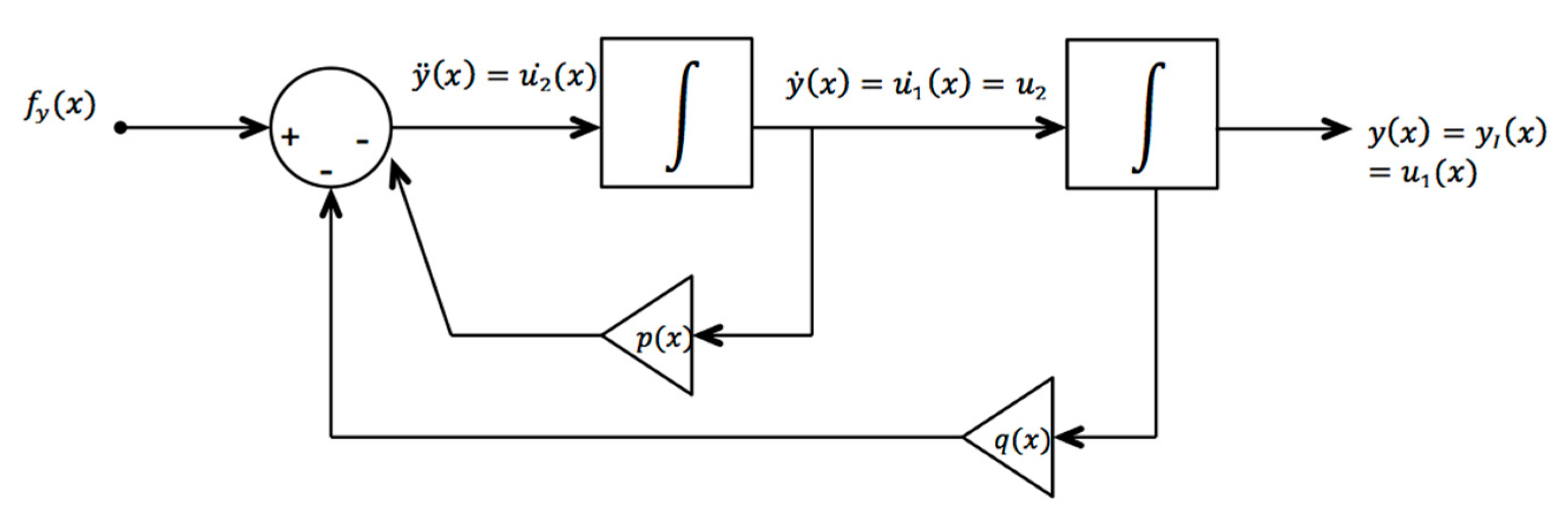
The feedback diagram of
Figure 1 presents the usual depiction of the second-order, linear, differential Equation (1). It includes two integrators, a summing box on the left, two amplifiers representing the variable coefficients
and
, and the nonhomogeneous driving function
. This is a format widely used with simulation software. Note, for example, that at the output of the summing box,
is as required.
An inherent alternative description, known as the state variable approach, is simultaneously indicated in
Figure 1. For this case, the second-order system is evaluated as two first-order equations in terms of the state variables
and
through the following transformation:
or in matrix form:
By renaming the vectors and matrices within Equation (5), the standard, variable-coefficient linear system canonical form description for this single-input, single-output (SISO) case is expressed as
Matrix
is the companion matrix of the corresponding characteristic polynomial of Equation (1), and the standard general solution to equations (5) and (6) [
11] (pp. 114–118), [
12] (pp. 74–75) is obtained from the fundamental or state transition matrix
as
The roman numeral superscript, I, emphasizes that the matrix relates to System One. This result in Equation (7) is also the variable coefficient version of Duhamel’s Formula [
13] (p. 149) and exhibits the zero-input and zero-state responses for the state vector
and single input
, respectively, in the two terms on the right-hand side. The 2 x 2 state transition matrix of Equation (7) for the initial-value problem of Equation (1) is, more specifically,
where the four elements
are only nonzero for
for initial-value problems. Finally, since we are only interested in
in Equation (1), the top row of Equation (7) provides the general solution to Equation (1):
Here, the ) initial conditions have been replaced by those for and as per Equation (4). Hence, whenever a state transition matrix can be found for a system, its two top row elements and provide the solution to Equation (1) by means of Equation (9).
2.2. System Two
A more general second-order linear system description for the SISO case compared to Equation (5) has the following state space description (with
):
and
A solution for this system through Equations (7) and (8) is not available in the general case of arbitrary
, where
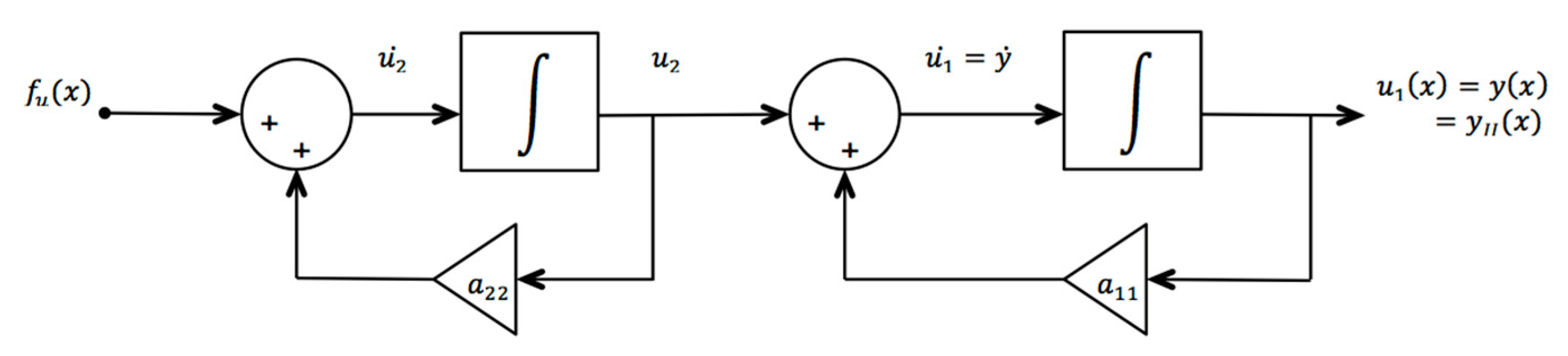
. However, since this general system has an overabundance of variable attributes for the purposes of matching System One, modifications can be implemented that guarantee the obtainability of a state transition matrix, as in Equation (8). Therefore, further simplification is imposed, as shown in
Figure 2.
The most important change for System Two is that has been set to zero. The resulting triangular form for ensures that it can be readily calculated from its definition as a fundamental matrix, , where the roman numeral II denotes System Two. A more extensive comparison of Systems One and Two reveals that for , the specific value of component drops out of the analysis and can thereby be replaced by a nonzero constant chosen to be one for simplicity. Similarly, the general components provide an unnecessary complication for solutions to System One and are replaced by constant values of zero and one, respectively.
2.3. Solutions for System Two
The differential equation solutions to System Two are obtained next, followed by the derivation of conditions necessary for their transference or application to System One.
The state-space description of System Two then becomes
or
The resulting state-transition matrix elements required for solutions, as previously noted in Equations (7) and (9), are summarized in the following theorem:
Theorem 1. A general 2 x 2 fundamental matrixfor the second-order system of Equation (12), valid over the intervaland to be used with initial conditionsand, is given by its four matrix elements:wherewhereand In summary, for System Two,
From Equation (20), the state-space solution for System Two analogous to Equation (7) for System One is
for the elements defined by Equations (14) to (19). Since we are primarily interested in
, the top row of Equation (21) shows the final desired solution for System Two:
2.4. Equalization of Systems One and Two
A direct comparison is made between
Figure 1 and
Figure 2, in order to apply the results of Equations (20)–(22) to System One. Using System Two, we see that
,
and
The differentiation of Equation (25) and comparison with Equation (24) shows that
from which we have a System Two description in terms of its output
and its derivatives
In order for System Two of
Figure 2 to provide the same input/output behavior as System One and Equation (1), the following equivalences must hold from Equation (27):
and
If the component values of System One are to be brought into System Two, then, from Equations (28) and (29), for known
and
,
and
Therefore, the determination of the proper choices for System Two coefficients and that ensure equivalence with System One comes from the Riccati equation solution of Equation (32), together with Equation (31).
2.5. Application of System Two Solutions to System One
The general solution to the differential equation describing System Two, Equation (22), shows the homogeneous solution with arbitrary constants in terms of the state-variable initial conditions and the particular response due to the driving function. For given
and
, the resulting matrix elements are presented in equations (14) through (19) and summarized in the complete state transition matrix of Equation (20). Then, this general solution will also apply to System One if the appropriate equivalent coefficients
and
resulting from the given
and
of Equations (31) and (32) are incorporated in the
and
matrix element calculations of Equations (14) through (19). These must be combined with the driving function equivalence of Equation (30) and the conversion from state-variable initial conditions to those originally posed for output
and its derivative in System One. Hence,
and, from Equation (25),
With these equivalents, together with that of Equation (30), Equation (22) becomes
For matrix elements calculated appropriately, that is, through the additional relations of Equations (31) and (32), the System Two solution will match that of System One. If a final comparison is made between Equation (35) and Equation (9), then solutions for System One can be readily identified as depending on System Two matrix elements as
and
Therefore, for resulting system equivalence, the impulse response functions for both systems are seen to be identical, and the matrix elements differ whenever the initial value of the System Two component resulting from the Riccati equation equivalence process of Equation (32) is nonzero.
In summary, when the System Two matrix elements and are calculated via Equations (14) and (19) using the appropriately chosen functions and that result from the System One, System Two equalization process of Equations (28) to (32), they provide the System One counterpart matrix elements necessary and sufficient for solutions to that system. Upon completion of this process in what follows, and Equation (35) solutions apply to either system.
2.6. System One Solutions from the Riccati Equation Connection
It has been shown that System One solutions can be constructed from readily calculable System Two matrix elements as per Equations (36) and (37) and Equations (14) through (19). Therefore, we must now search for appropriate System Two coefficients
and
that correspond to System One
and
from Equations (31) and (32). An important aspect of Equation (32) is the recognition that various functional forms, such as
or
used in Equations (20) and (35), present solutions to differential equations in the form of Equation (1) for the specific coefficient interrelations
or
, respectively. Note that the former case of constant
has been previously analyzed from a related yet different viewpoint in [
1]. Similarly, other choices, such as
or
, also lead to comparable coefficient interrelationships and equation solutions. However, it is advantageous and more systematic for some situations to deal with the Riccati equation connection for
of Equation (32) by means of a transformation to a new function,
, which results in
. For known
and
, and by defining
this becomes
The quantity
(x) is the negative of the Schwarzian derivative for Equation (1) and plays an important role in more generalized studies of differential equations [
14].
Solutions for
or
are the main links between Systems One and Two, and the relations among the feedback coefficients are
and, from Equation (31),
Assuming that
solutions are obtained from Equation (39), we can recast the matrix elements from Equations (14) through (19) in terms of the calculated
and known
by using
Here,
and
follow the previous format of small letter-capital letter integral definitions, as in Equations (15) and (17). Similarly,
and the System Two state transition matrix
in Equation (20) is
When the top two matrix elements of Equation (46) for calculated
are substituted into Equation (35), the System One solution,
, results in
Note that, here,
for Equations (35) and (47) is given from Equation (40) as
An additional note of concurrence for the
and
matrix elements of Equation (46) is provided by the reduction of order technique for independent solutions, since
and
exactly adhere to the well-known interconnecting result [
15] (pp. 171–172) of
Here, the constants can be seen to be
and
from Equation (A2) of
Appendix A, thereby providing agreement for the upper-right matrix element expression.
4. Equations Solvable by Quadrature Resulting from Particular Riccati Equation Solutions
Although it is presently not possible to solve the Riccati equation of Equation (39) in closed form for any function , i.e., for any choice of coefficients and , particular solutions exist for specific forms of the function defined by Equation (38). Furthermore, any such particular forms for also interrelate and hence limit the resulting and possibilities that allow a corresponding quadrature solution. Groups of second-order, linear differential equations characterized by the same form for that function then share a common quadrature solution description determined by Equations (38) through (48).
An alternative but related view of Riccati equation solutions is provided by the transformation of
in Equation (39) to another function
through
, which results in
If two linearly independent solutions
and
can be found to Equation (55), then the general form for Equation (39) for
is determined by [
16] (pp. 239–242)
where
Although finding exact solutions to Equation (55) in the general case is usually as difficult as solving Equation (39) directly, simultaneous observations for both the Riccati equation and the corresponding Helmholtz equation can be insightful, as discussed with the normal form approach in
Section 7.
In the following, three groups of linear, second-order, variable coefficient, ordinary differential equations are presented. The first corresponds to the function of Equation (38) chosen to be constant, and hence readily admitting a solution to Equation (39), and the next two groups each assume a special form for the or Riccati equation solution. In all cases, either function or then determines the relationship between coefficients, that is, initially chosen and subsequently calculated , through Equations (38) and (39). This resulting coefficient pair then defines the explicit version of Equation (1) describable by the quadrature solution of Equations (38) through (48).
4.1. Group One: Quadrature Solution to Equation (1) Corresponding to the Constant
If the function of Equation (38) is constant, then the Riccati equation of Equation (39) is readily solvable for functions , as summarized in the ensuing proposition.
Proposition 1. For the coefficientsandof Equation (1) assuming values such that functionof Equation (38) is constant, then the following results for Riccati equation solutionare valid over intervalwith real constant c.
Category 1(a): For,
Category 1(b): For,
Category 1(c): For,
Proof of Proposition 1. For category 1(a), . For Equation (39), the separation of variables and , followed by partial fraction expansion and integration over leads to Equation (57). Alternatively, the transformation of to resulting in Equation (55) leads to cosh and sinh function solutions for that equation. Equation (57) then results from Equation (56).
For category 1(b), . The direct integration of either Equation (39) or Equation (55) leads to Equation (58).
For category1(c), . As in case 1(a) above, the separation of variables with partial fraction expansion and the direct integration of Equation (39) leads to Equation (59). Alternatively, from Equation (55), the resulting cos and sin solutions inserted in Equation (56) reproduce Equation (59).
The families of equations solvable from this methodology for the function constant are determined in each category by the Equation (38) definition. For each choice of coefficient , the corresponding second coefficient is determined as follows:
Category 1(a),
:
Category 1(b),
:
Category 1(c),
:
Then, each and pair defined by these relations results in a form of Equation (1) whose quadrature solution is given by Equation (35), as determined by the following matrix elements calculated from Equations (40) through (46) for the results of Equations (57)–(59).
Here, as in Equation (44), is the integral of arbitrarily chosen . These elements are used in each case in Equation (35) to solve Equation (1) over for initial conditions and . Note that the presence of vanishes algebraically from the final result of Equation (35), since , , , and are the only elements directly determining the final solution for differential equations of Group One.
Despite the straightforward nature of the resulting matrix elements of Equations (63) to (68), the form of the solution generally provided by this method for this group can introduce computational difficulties due to the logarithmic functions that are present. For example, for Category 1(c) and depending on the solution interval, will have multiple zeroes and negative regions occurring within its argument, which can halt the calculation. Hence, alternative computational strategies may be required at times. □
Constant Coefficient Equations
A last point of significance for this section is that all constant coefficient ordinary differential equations in the form of Equation (1) are included within Group One. That is, for constants and , the quantity will determine which of the three previous categories provides the solution, depending on whether constant is positive, negative, or zero.
4.2. Group Two: Quadrature Solution to Equation (1) Corresponding to
Given the Riccati equation for
, Equation (39), and the structure of the function
of Equation (38), the fact that
is an immediate solution of Equation (39) for
suggests a trial solution of the form
that will also satisfy this equation for known, real, nonzero function
, which is arbitrary within some limitations to be discussed. From Equation (40), this is equivalent to
Due to its arbitrary character, the function
will serve to define families of possible real coefficients
of Equation (1) amenable to the System Two solutions of Equations (40) to (48). The coefficient
is assumed to be given. Upon substitution of the
and
terms from Equation (69) into Equation (39), it is seen that coefficients
for which Equation (69) holds must satisfy the additional Riccati equation
A solution to this Riccati equation leads to the following theorem.
Theorem 2. For a given real coefficientof Equation (1) and the trial solution of Equation (69), a corresponding functional form for feedback elementthat provides particular solutions forof Equation (39) and hence direct application of the solution methodology of Equations (35) to (37) and equations (40) to (48) to Equation (1) is obtained asfrom which coefficientfollows asHere,are initial values,is defined by Equation (44), andis defined by Furthermore, the complementary state-variable matrix elements for utilization in Equation (35) (or Equations (46) and (47)) areand The value ofto be used with these matrix elements in Equation (35) is.
The Proof of Theorem 4.2.1 follows in Appendix A. In summary, a family of equations in the form of Equation (1) has been established in this section for arbitrary coefficient
and the second coefficient
determined from Equation (71), together with the matrix elements of Equations (73) and (74) comprising each family’s solution from Equation (35). Individual family members are ascertained by the specific choices for the initial parameter
and function of proportionality
of Equations (69) and (72). The great latitude in choosing function
presents a wide variety of possibilities for interrelating coefficients
and
through Equation (71). For example, the choice of
leads to versions of the
result discussed in
Section 2.6, with specific details being dependent upon the value of
. However, as seen in Equations (71) and (72), choices for the function
should preclude those that would introduce singular points within the solution interval. Conversely, the solution interval
should be adjusted accordingly for a specific
to avoid problematic regions for
,
,
,
, and
.
4.3. Group Three: Quadrature Solution to Equation (1) Corresponding to
Another group of solutions for
of the Riccati Equation (39) is obtained from a trial solution of the form
which is equivalent to
. Again, this is motivated by the fact that
is an exact solution to Equation (39) for the case of
. The coefficient
is real-valued and arbitrary, but assumed to be known, and here,
is again a real-valued and arbitrary known function of proportionality that will be assumed to be strictly positive. Moreover, only positive real resulting
functions are included. This will restrict consideration in this case to equations of form (1) with real coefficients only.
In parallel to what was seen in
Section 4.2, the use of Equation (75) in Equation (39) results in the Bernoulli equation [
17] (p. 49)
of power
for the nonlinear
term. The solution of this equation leads to the next theorem.
Theorem 3. For a given real coefficientof Equation (1) and the trial solution of Equation (75), a corresponding functional form for feedback elementthat provides particular solutions forof Equation (39) and hence direct application of the solution methodology of Equations (35) to (37) and Equations (40) to (48) to Equation (1) is obtained asfrom whichfollows asAdditionally, the corresponding state-variable matrix elements for Equation (35) areand As in
Section 4.2, the arbitrariness of
is limited to strictly positive continuous functions not introducing singularities to any of the differential equation quantities of Equations (77)–(79) over the solution range
, x).
In summary, given the real coefficient
, adjunct (positive only) function
, and positive initial value
all of which are arbitrary within the restrictions cited, Equation (77) provides the resulting form of the positive-only
coefficients corresponding to the assumption of Equation (75) and thereby appropriate for Equation (1) to be solvable by means of the matrix elements of Equations (78) and (79) in Equation (35). Note that the initial value constant
takes on the value
from Equations (40) and (75). As in
Section 4.2, and despite limitations, the range of possibilities encompassed by the arbitrary function
and parameter
offers a wide array of equations in the form of Equation (1) with quadrature solutions.
5. Application to the One-Dimensional Helmholtz Equation
The one-dimensional Helmholtz equation is of importance to many branches of physics and engineering, often representing time-independent wave behavior that occurs in quantum mechanics, electromagnetics, and optics [
18] (pp. 31–44), [
19] (pp. 206–229). This equation is often dealt with through the WKB approximation in the Physical Sciences [
20] (pp. 27–37), which can provide accurate results comparable to those from more exact methods [
21]. The Helmholtz equation and its solution also have bearings on the diffusion equation and related studies [
22].
Since the nonhomogeneous version of this equation is of the form
the families of specific differential equations with quadrature solutions obtained in
Section 3 and
Section 4 apply directly for the choice of coefficient
, thereby supplying additional non-approximate solutions. Although wave investigations using this equation are usually posed as boundary value problems, the initial value version developed here can be interpreted as a portrayal of unidirectional wave propagation over region
in infinite media with spatially varying characteristics, as indicated by non-constant
. With this interpretation as the background, exact propagation results for Equation (80) can be taken from Sections Three and Four and are summarized in the following.
Given that
in Equation (1) here, the relevant Helmholtz coefficients
leading to the subsequent quadrature solution are determined from Equations (38) and (39) by
for given, real arbitrary
. The corresponding System Two feedback elements of
Figure 2, from Equations (40) and (41), are
from which constant
. The quantity
of Equation (43) then determines the two pertinent matrix elements of Equation (46) to be
The accompanying quadrature solution for Equations (83) and (84) follows as in Equation (47) by inserting these matrix elements into Equation (35) to give
There are many potentially useful versions of the Helmholtz equation available, with solutions from Equations (81) to (85) stemming from the arbitrary nature of within Equation (81).
For this Group One case, from Equation (38) for
,
Constant represents a simple and elementary Helmholtz equation for which the feedback diagram method provides a relatively complicated solution. Nevertheless, the formalism provides three possibilities for the constant of Equation (86) and for parameter being any real constant:
Category 1(a), : given by Equation (57);
Category 1(b), : given by Equation (58);
Category 1(c), : given by Equation (59).
The corresponding matrix elements
and
are given by the three pairs of Equations (63) and (64), (65) and (66), and (67) and (68) for
from Equation (44). The System Two feedback elements are then
from Equations (40) and (41) for
, and hence initial constant
. Finally, the System One solution
is obtained from Equation (35) using the matrix elements whose values are outlined above.
Clearly, direct and elementary methods for solving the Helmholtz equation under Group One conditions of constant coefficient are preferable to the equivalent results obtained here.
The relevant Helmholtz
coefficient is taken from Equation (71) as
with
and
, where
and
is defined by Equation (72). Real function
, assumed to be nonzero over
and initial constant
are both assumed to be arbitrary, provided that no singularities are introduced for that region in the denominator of equations such as Equation (88) by these choices. The System Two feedback elements are as in Equation (87), with
. The matrix elements
and
are determined by Equations (73) and (74) with
:
As before, the substitution of these matrix element expressions into Equation (35) generates the System One solution family for the corresponding family of Helmholtz equations.
In this case,
for Helmholtz Equation (80) is obtained from Equation (77) as
with
for arbitrary but strictly positive function
where
The initial constant
is then
, which is used with the following matrix elements in Equation (35) to provide the
solution. The first matrix element is from Equation (78) with
:
Using Equation (92) in Equation (79), again with
, gives the second matrix element:
6. Application of Series Methods for Riccati Equations without Known Particular Solutions
For known
and
of Equation (1), the Riccati Equation (39) connection between Systems One and Two only differs from one equation or system under study to another by the (negative) Schwarzian derivative Equation (38). Hence, it is effectively universal in both form and solution. For Riccati equations without known particular solutions that would otherwise permit and guide further analysis, a potentially useful alternative comes from a series approach, such as the single-variable Adomian Decomposition Method (ADM) [
8]. This versatile method compartmentalizes the analysis of nonlinear ODEs into the general form
where
is a chosen invertible linear operator,
is the remaining part of linear operations, and
is the nonlinear operator, all of which act on
, together with the driving function taken from Equation (38). Due to the simplicity of Equation (39),
,
,
, and the solution is abstractly
where inverse operator
and the homogeneous solution for
is
which is equal to constant
. We also define integral
) as the (negative) Schwarzian derivative integral
The solution
is assumed to be determined by the infinite series
. Similarly, the nonlinear component is assumed to be describable by
for the Adomian polynomials
. These are defined for all
by
Although the higher Adomian polynomials become quite lengthy and calculationally intensive, n-term approximations for them can provide accurate results with relatively rapid convergence for a judicious choice of operators L and R in the general case [
9,
10]. However, for
, only two
derivatives are nonzero. In the original Adomian recursion scheme [
8], the initial series element for
is chosen to be
Note that the initial constant
is either found from Equation (48) for known
or is left undetermined as an arbitrary constant. From Equation (95) and the
Adomian polynomial expansion above, the
function series components are
For Equation (39), the first six Adomian polynomials are
From the uncomplicated nature of Equation (39), the higher Adomian polynomials are simplistic in form, since for
where a Kronecker
demarcates the i = j terms. The convergence of the Adomian Decomposition series has been examined and confirmed by several authors [
23,
24,
25,
26]. For Equation (39), from the recursion scheme of Equation (99), the first four
elements using the Adomian polynomials of Equation (100) are
Therefore, an overall solution
is shown to be a series of terms composed of increasingly multiple integrals of the negative Schwarzian derivative plus a constant for the differential equation. This series solution is most appropriate for Riccati equations without identifiable particular solutions for
, unlike those shown in the three categories of
Section 4. The convergence of the
series can be examined through a ratio test [
25] by checking whether
for an appropriately chosen norm, which can also determine the radius of convergence of the series.
In summary, the implementation of the algorithm of Equations (99) through (102) provides a general solution mechanism for Equation (39), and the link between a system under study and a second system, which provides solutions to it through Equation (47) and the matrix elements of Equation (46). This link is unchanging in form, varying only through the details of the negative Schwarzian derivative. Hence, the series expansion and its corresponding integral series, defined by Equation (43) and used directly in Equation (47), extend the applicability of the feedback diagram method in principle to all differential equations in the form of Equation (1), for which a (uniformly) convergent series can be obtained over interval . However, this formal solution will have practical utility that is highly dependent upon series convergence being adequately rapid and regions of convergence being largely unrestricted.
ADM Implementation
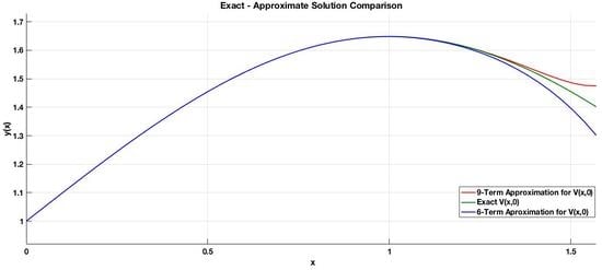
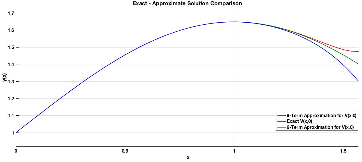
Example 2. A simple example illustrates these results. Considerfor unspecified driving function, initial conditions, and solution interval. The negative of the Schwarzian derivative of Equation (38) is simplyNote that the solution to Equation (103) falls within the Group One category presented in Section 4.1 for constant, in which the Equation (39) solution isAs such, the exact solution to Equation (103) is obtainable either from Equation (35) together with equations (63) and (64) or from Equation (47) together with Equations (43) and (44), with the final result in either case being For series approximation, the ADM algorithm under these conditions, together with, leads to the following sequence of Adomian polynomials: From these Adomian polynomials, sixelements follow from Equation (99):which are seen to duplicate the MacLaurin Series forfor its first six terms. Note, however, that the region of convergence for this series is tightly restricted to. The integration of this last set of elements as per Equation (43) gives the first six elements of,
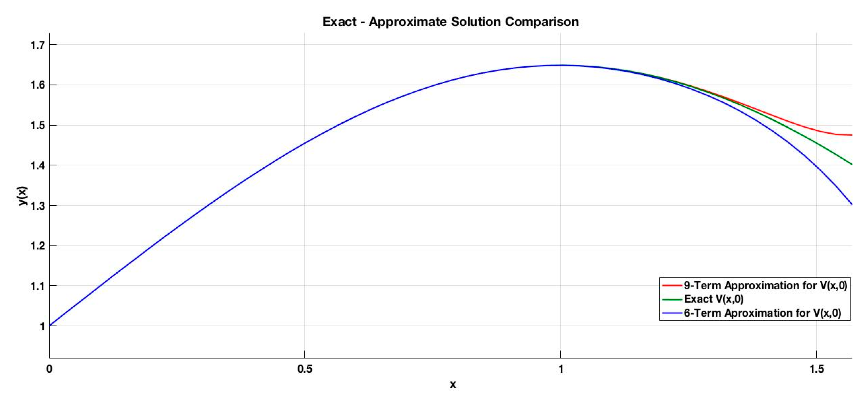
for subsequent usage in theandmatrix elements of Equation (46). From the known tanh(x) result, Equation (107) becomesin the limit within regions of convergence. Ultimately, this appears as powers ofdue to exp(V) and exp (-2V) in Equations (46) and (47) for describing the two matrix elements. Some numerical details more fully characterize this illustration. The six-term approximate solution obtained by the substitution of Equation (107) in Equation (47) is contrasted with the exact homogeneous solution of Equation (103) in Figure 3. Also included is a nine-term approximate solution. For this comparison, the initial valueswere both chosen to be one. From the figure, for the interval (0, 1.57), the three solutions are found to be within much less than one per cent of each other up till x = 1.2. At x = 1.5, the deviation of the nine-term approximation is about 2.2% above the exact solution and that of the six-term approximation is about 4.1% below. The positive versus negative deviations are generated by the positive versus negative sign of the highest order term in each approximation, hence the bracketing of the exact result, and the series method ceases to apply atThe accuracy of the approximate results are mediocre, with improvement requiring the generation of additional terms or possibly the utilization of an alternate method.
Hence, although there is agreement for the Adomian Decomposition Method with previously determined results for this simple example, limitations on its practicality for solutions of Riccati Equation (39) not connected to particular solutions are seen to arise from issues of series convergence. The ADM has been chosen due to its power and flexibility to encompass a wide variety of equations. However, an alternative, such as Picard’s Iteration Method, also leads to a comparable series solution of multiple integrals of the Schwarzian derivative. Other choices are the Homotopic Analysis Method (HAM) [27] and the Homotopic Perturbation Method (HPM) [28], which often prove to be highly effective. These related approaches are widely used for nonlinear differential equations, and both employ a series of calculated functions in a series expansion with a homotopic expansion or imbedding parameter. Much as for the ADM, both methods employ linear and nonlinear equation components within their analyses. As the imbedding parameter varies from zero to one (analogous to a homotopy or continuous deformation from one topological surface or function to another), the series solution is altered from serving as a solution to the linear component equation to solving the nonlinear one. Of further significance are the facts that a small parameter is not required and that the series functions are calculated from a succession of linear equations. Additionally, the application of HAM or HPM can often result in convergence requiring only a few iterations [29]. Nevertheless, for any iteration scheme, the practical application of the feedback diagram method for an infinite series solution forof Riccati Equation (39) is strongly contingent upon both sufficiently unrestricted regions of convergence and a sufficiently rapid rate of series convergence. 7. Conclusions and Discussion
In summary, a novel feedback diagram-based methodology has been constructed and presented for the generation of equations solvable by quadrature, together with their corresponding solutions, for those adhering to the standard form for second-order, linear differential equations, as in Equation (1), with its coefficients
and
and initial conditions. Solutions of these equations (or systems) can be acquired from another system, specifically designed to produce such results upon the determination of solutions for feedback elements
or
of the Riccati equation link between the two systems. In
Section 3, families of differential equations with solutions were generated by calculating
coefficients from choices for arbitrary
and
In
Section 4, particular Riccati equation solutions for
or
were determined by either assuming constant values for the Schwarzian derivative or specific assumed forms for these feedback elements in terms of
and
Under either set of assumptions,
relations were determined, which describe families of solvable equations, together with their corresponding quadrature solutions. In each case, members of these families were specified by choices for an arbitrary function and parameter. In
Section 5, the outcomes of the previous two sections were extended to the physically important Helmholtz equation by limiting
to zero. Finally, in
Section 6, the Adomian Decomposition Method was employed to provide a Riccati equation series solution for all differential equations (1) not overtly dependent upon particular Riccati solutions for
or
The overall result, which is an infinite series in terms of multiple integrals of the Schwarzian derivative, formally provides a quadrature solution to any linear, second-order differential equation (1). However, important practical limitations may arise due to restrictions on solution regions of applicability and/or slow rates of convergence.
Two parallel and related developments, which lead to results quite similar to those of the feedback diagram method, will now be compared and considered. The first method comes from the normal form of Equation (1) [
2,
3], in which a product form of solution
is assumed with the further assumption of
using Equation (44). If these are substituted in Equation (1), its normal form is derived as
together with appropriate initial conditions. The negative Schwarzian derivative definition for
of Equation (38) has been utilized, and the solution to Equation (1) follows from Equations (108) and (109) as
The normal form approach is usually presented as relying upon a solution to the nonhomogeneous Helmholtz equation of Equation (109). However, for arbitrary coefficient
, this is often as difficult to solve as the original Equation (1), although some of the Helmholtz equation results of
Section 5 derived here may be helpful. Two independent homogeneous solutions to Equation (109),
and
would be required, or at least one would need to be determined, followed by a reduction of order to generate the second. These two could then be used to construct an impulse response or Green’s function to encompass the nonhomogeneous Equation (109) through the relation [
16] (p. 113)
This is the role played by
in
Section 2 for the feedback diagram method.
An alternative to solving the homogeneous version of (109) follows the Riccati equation procedure of Equation (39) utilized in
Section 2. That is, with the substitution (recall Equation (55)) of
, this homogeneous version is seen to revert back to Equation (39) since
Any resulting solutions for
could then be converted to homogeneous
solutions by
using the
definition of Equation (43). A reduction of order for a second solution and the impulse response of Equation (111) would then accommodate the nonhomogeneous version of Equation (109), and a complete
solution would result as per Equation (110). Overall, Equation (112) serves as a connection between the normal form and the feedback diagram methods, making the Riccati equation solutions of
Section 4.2,
Section 4.3,
Section 5, and
Section 6 available to each approach.
A second method, which parallels the development here, is that of Badani [
5], who reduces the general form of Equation (1) to a corresponding first-order nonhomogeneous equation through an insightful grouping of terms and defining of functions. The derived equation can be solved directly by an integrating factor, which also includes a key term which is itself a solution to a Riccati equation. Through a comparison to the method presented here, that key term can be identified as
and the associated Riccati equation as Equation (32). Hence, the Badani method and the method presented here both arrive at the same result, but by different routes. An advantage of the feedback diagram method developed here is that in utilizing Equation (39) for
rather than Equation (32) for
, the Schwarzian derivative can be used to systematically generate equations and their quadrature solutions, as in
Section 3.1; serve as a compact and useful marker to classify or characterize second-order linear differential equations with solutions, as in
Section 4.1; or develop series solutions formally extendable to all versions of Equation (1), as established in
Section 6. Badani presents several well-chosen examples illustrating his approach for particular choices of the coefficients
and
leading to particular Riccati solutions. However, the use of function
, Equation (39), and the negative Schwarzian derivative of Equation (38) can together provide a broader, more systematic perspective, as has been demonstrated by the generation of families of equations with solutions in
Section 3,
Section 4,
Section 5 and
Section 6.
Finally, the presentation of the feedback diagram method here outlines a pathway for extending these results so as to obtain comparable families of equations with quadrature solutions for third-order and even higher-order linear differential equations.


