Abstract
A non-intrusive approach coupled with non-uniform rational B-splines based isogeometric finite element method is proposed here. The developed methodology was employed to study the stochastic static bending and free vibration characteristics of functionally graded material plates with inhered material randomness. A first order shear deformation theory with an artificial shear correction factor was used for spatial discretization. The output randomness is represented by polynomial chaos expansion. The robustness and accuracy of the framework were demonstrated by comparing the results with Monte Carlo simulations. A systematic parametric study was carried out to bring out the sensitivity of the input randomness on the stochastic output response using Sobol’ indices. Functionally graded plates made up of Aluminium (Al) and Zirconium Oxide (ZrO) were considered in all the numerical examples.
1. Introduction
Composite materials are widely used in a large variety of structures due to their high strength to weight ratio and excellent thermo-mechanical and corrosion resistance properties [1,2,3]. On the other hand, composite materials can be engineered to achieve a varying spatial composition profile and, hence, arrive at the required properties at specific locations. Such inhomogeneous materials, consisting of two or more different materials, are known as functionally graded materials (FGM). Functionally graded materials can be fabricated by varying the elastic modulus from one phase to another in one or more directions. Some applications of FGM include rocket heat shields, electrical insulation in metal/ceramic joints, dental implants, and bone replacements [4]. The FGM fabrication process results in inherent randomness, since the gradients of the constituent materials are to be varied continuously in the space along with the physical material properties. Therefore, the analysis of FGM using deterministic approaches will not accurately predict actual behaviour. The inherent uncertainties existing in the system are required to be considered while estimating the system response. Thus, structures involving functionally graded materials are required to be modelled and analysed using stochastic analysis [5].
One straight forward approach to quantify the effect of randomness on the output response is to use a direct Monte Carlo simulation (MCS) approach. However, given that the MCS requires a sufficiently large number of samples, typically 10,000, it becomes computationally intractable. To alleviate this issue, the stochastic finite element method was found to be the most common and promising tool to study the stochastic response. Different variants of the stochastic finite element method include the probabilistic finite element method [6], the weighted integral method in stochastic finite element analysis [7], the spectral stochastic finite element method [8], and the stochastic finite element method based on perturbation technique [9], to name a few. A comprehensive discussion of stochastic finite element methods is given in [10].
A stochastic perturbation technique was adopted to study the free vibration characteristics of FGM plates in [11,12]. The spectral stochastic isogeometric analysis (SSIGA) using the first order deformation theory was implemented by Keyen Li et al. to obtain the static response of the FGM plates [13]. Chiba et al. [11], addressed the randomness in the thermal conductivity and coefficient of linear thermal expansion of the FGM plates. The analysis was performed by considering the thermal properties to be distinct for each layer. Stochastic finite element analysis using artificial neural networks (ANN) coupled with higher-order-zigzag theory (HOZT) was presented by R.R. Kumar et al. [14]. In this study, it was shown that the uncertainty in the input parameters has significant effects on the higher order modes of the buckling analysis [14]. The size-dependent effects on thermal buckling and post-buckling behaviours of the imperfect micro FGM plates with porosity is presented using isogeometric analysis in [15]. The seventh order shear deformation plate theory was employed to capture the size-dependent phenomenon. Shaker [12] studied the stochastic free vibrations of FGM plates using the third order shear deformation theory, with uncertainties in the constituent material properties and the volume fraction index. However, a subtle drawback of this approach is that it is limited to small input variance, typically less than 20% [16]. Kumaraian et al. [17] employed a cell-based smoothed discrete shear gap method to study the stochastic free vibration characteristics of functionally graded material plates. The input random field was represented by using the Karhunen–Loéve (KL) expansion, and a polynomial chaos expansion was used to represent the stochastic output response. The critical buckling behaviour of the the plate due to the varying thickness and presence of cracks was addressed using the phase field theory coupled with third order shear deformation theory [18]. Sepahvand et al. [19] studied the stochastic free vibration characteristics of orthotropic plates with uncertainty in elastic moduli using the generalized polynomial chaos expansion (gPCE) to represent both the uncertainty in input as well as in the output. The sensitivity analysis for low-frequency vibration and low-velocity impact of the FGM plates was presented by Karsh et al. [20]. The equilibrium and stability equations of FGM plates for working in the high temperature conditions were formulated by Tran et al. [21]. The optimisation using hybrid evolutionary firefly algorithm of the FGM plates subjected to thermo-mechanical loading was demonstrated by Lieu and Qui X [22].
In this work, the influence of the randomness in the material properties, particularly, Young’s modulus and density on the uncertainty in the static bending and free vibration characteristics of FGM plates were studied using a non-intrusive approach. The salient feature of this approach is that it does not require any modification to the existing code. However, to capture the uncertainties, the forward solver has to be used as a black-box, which has to be computationally efficient. Hence, in this paper, we used the non-uniform rational basis spline (NURBS)-based isogeometric analysis framework for the spatial discretization, and the plate kinematics is based on the first order shear deformation theory. The results from the proposed framework are validated against the Monte Carlo Simulations with a sufficiently large number of samples. The sensitivity of the material randomness on the output characteristics are studied using Sobol’ indices.
The rest of the paper is organized as follows: an overview of the functionally graded material plates, and the first order shear deformation plate theory is presented in Section 2. Section 3 presents a brief discussion of the isogeometric analysis employed in this study. The non-intrusive spectral approach is presented in Section 4. The influence of the material randomness on the static bending and free vibration of functionally graded plates are presented in Section 5. The results from the present framework are compared with the brute-force Monte Carlo simulations. The sensitivity of the random variables on the stochastic output response was systematically studied. This is followed by conclusions in Section 6.
2. Analysis of Functionally Graded Panels
2.1. Effective Modulus and Poisson’s Ratio
In this study, a rectangular composite plate made of ceramic and metal is considered for simulations. As shown in Figure 1a, the dimensions along the in-plane directions (x, y) and along the thickness (z) direction are indicated by , and h, respectively. The material on the top surface of the plate is ceramic rich and is graded to metal towards the bottom surface of the plate, according to a power law. The effective properties of the plate made of functionally graded materials can be estimated by employing either the rule of mixtures or the Mori–Tanaka homogenization scheme.
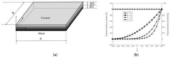
Figure 1.
Functionally graded rectangular plate: (a) geometry and (b) volume fraction of ceramic and metallic phases through the thickness of the plate for different gradient indices.
Let denotes the volume fraction of the constituent phase, where the subscripts c and m refer to ceramic and metallic phases, respectively. The total volume fraction of ceramic and metal phases is related as . Furthermore, the volume fraction of the ceramic () is given by Equation (1):
where n is known as the volume fraction exponent , or the gradient index. The composition of the ceramic and the metal varies linearly when 1, whereas, 0 indicates a fully ceramic plate. Any other value of n yields a composite material with a smooth transition from ceramic to metal, as shown in Figure 1b. In this study, the Mori–Tanaka homogenization scheme is adopted to compute the effective Young’s modulus and Poisson’s ratio.
According to the Mori–Tanaka homogenization scheme, the effective Young’s modulus () and Poisson’s ratio () are computed using the effective bulk modulus () and the effective shear modulus (), as [23]:
where the effective bulk and shear modulus can be estimated using the relations mentioned below:
and are the bulk modulus and and are the shear modulus; of the metal and ceramic materials, respectively, and
2.2. First Order Shear Deformation Theory
The displacements along the x, y and z directions at a point in the plate (see Figure 1a), indicated by , can be expressed in terms of the mid-plane displacements and independent rotations in the and planes, respectively, as:
The strain field in terms of mid-plane deformation are given by:
The mid-plane (), bending (), shear () strains in Equation (10) are:
where the subscript "comma" represents the partial derivative with respect to the succeeding spatial coordinate. The resultant membrane stress () and the resultant bending stress () can be expressed in terms of the membrane strains, and bending strains through the following constitutive relations:
where the matrices and indicate the extensional, bending-extensional coupling, and bending stiffness coefficients, which are defined as:
Similarly, the transverse shear force is related to the transverse shear strains () as:
where is the transverse shear stiffness coefficient, are the transverse shear coefficients for non-uniform shear strain distribution through the plate thickness. The stiffness coefficients are defined as:
where the modulus of elasticity () and the Poisson’s ratio () are estimated using Equation (3).
The total strain energy (U) of the functionally graded plate can be estimated as:
where indicate the vector of degrees of freedom. Furthermore, the strain energy function in Equation (22) can be rewritten as [24]:
where is the linear stiffness matrix. On the other hand, the kinetic energy of the plate is given by:
where and is the mass density which varies along the thickness direction. Moreover, considering the thermal field results in the in-plane stress, . The external work due to the in-plane stresses developed in the plate in the presence of a thermal load is given by:
The governing equations of motion can be obtained by considering the Lagrange equations of motion mentioned below
The governing equations obtained using the minimization of total potential energy in Equation (26), are solved using the Galerkin finite element method. Therefore, the simplified finite element equations can be written as:
Static bending:
Free vibration:
where
are the stiffness matrix, the mass matrix and the force vector, respectively, is the vector of degrees of freedom and are the strain-displacement matrix given by:
where n denotes the number of nodes.
3. Overview of Isogeometric Analysis
In this study, non-uniform rational basis spline (NURBS) basis functions are used in the finite element approximation. A brief introduction to NURBS is presented here, further details on their use in finite element method (FEM) are discussed in [25,26]. The key ingredients in the construction of NURBS basis functions are: the knot vector (a non decreasing sequence of parameter values, ), the control points, , the degree of the curve p, and the weight associated to a control point, w. The ith B-spline basis function of degree p, denoted by is defined as:
A degree NURBS curve is defined as follows:
where are the control points and are the associated weights. Figure 2 shows the third order non-uniform rational B-splines for a knot vector, . NURBS basis functions has the following properties: (i) non-negativity, (ii) partition of unity, ; (iii) interpolatory at the end points. As the same function is also used to represent the geometry, the exact representation of the geometry is preserved. It should be noted that the continuity of the NURBS functions can be tailored to the needs of the problem. The B-spline surfaces are defined by the tensor product of basis functions in two parametric dimensions and with two knot vectors, one in each dimension as:
where is the bidirectional control net and and are the B-spline basis functions defined on the knot vectors over an net of control points . The NURBS surface is then defined by:
where is the weighting function. The displacement field within the control mesh is approximated by:
where are the nodal variables and are the basis functions given by Equation (38). The transverse shear deformations are included in the formulation of the Mindlin theory for thick plates. In the Mindlin theory, the transverse normal to the mid surface of the plate before deformation remain straight but not necessarily normal to the mid surface after deformation. Based on this condition, the continuity requirement on the assumed displacement fields can be relaxed. However, for very thin plates, the following relations must be satisfied:
i.e., the shear strain must vanish in the domain as the thickness approaches zero. The lower order NURBS basis functions suffer from shear locking when applied to thin plates. Kikuchi and Ishii [27] introduced an artificial shear correction factor to suppress shear locking in a 4-noded quadrilateral element. In this paper, we employ the same technique to suppress the shear locking syndrome in lower order NURBS basis functions [28]. The modified shear correction factor is given by:
where n and are positive integers, is the diameter of the element equal to maximum or diagonal length of the element, h is thickness of the element and is the shear correction factor.
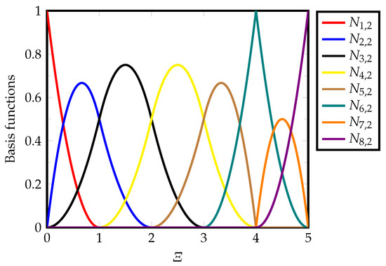
Figure 2.
Non-uniform rational B-splines, order of the curve, 2.
4. Non-Intrusive Spectral Projection
Let represents the response from a computational model, where denote the random input parameters of a probabilistic model, in which d indicates the number of random parameters. The randomness in the computational model could be due to randomness in the material, geometry, and/or the applied load. In this study, only the randomness in material properties is considered. Therefore, a finite variance of the output Y in the Hilbert space can be represented as:
where are the polynomial coefficients and denote the multivariate basis.
An orthonormal multivariate polynomial basis is selected for the polynomial chaos expansion. The orthogonal polynomials can be obtained using the monomials , and the Gram–Schmidt orthogonality condition.
Norbert Wiener first proposed [29] the polynomial chaos expansion (PCE) for Gaussian random input variables in terms of Hermite polynomials, which can be used to expand the random process with finite variance, known as the second order random process. These polynomials can approximate a given functional in the space and the convergence also happens in space. Therefore, polynomial chaos expansion theory can be applied to a wide range of real-time applications. The list of random distribution functions and their corresponding optimal orthogonal polynomials are listed in Table 1.

Table 1.
Wiener–Askey polynomials and their corresponding random variables; N is a finite integer.
The orthogonal polynomials are univariate, and the tensor product in the multi-dimension can provide multivariate orthogonal polynomials. Let us consider the second order random process denoted by the output variable Y, which is a function of random event . The polynomial chaos expansion using the Legendre polynomials can be written as:
where denotes the Legendre polynomials of order n and the independent random variable follows the uniform distribution and its dispersion around the mean is specified using the coefficient of variation (CoV). The polynomial chaos expansion is represented using the integrals, which are replaced by the summation in the discrete form. For practical applications, the infinite series in Equation (44) is truncated as mentioned below
where p indicates the highest polynomial degree and d denotes the dimensionality of the random input vector. The Legendre polynomials in general can be expressed as
where or whichever is an integer. A simplified form of Equation (44) considering N PCE terms is given by
The Legendre polynomial basis satisfies the following orthogonality property.
where represents the Kronecker delta and indicate the inner product in the Hilbert space determined by the support of the random variable, i.e.,
The coefficients in Equation (44) are obtained using the Galerkin projection. This implies Equation (44) is multiplied by every polynomial as shown below:
The residual error representing the output response, which is estimated using the PCE can be ensured to be orthogonal to the function space spanned by the PCE basis, through Equation (48). Equation (48) can be evaluated using the Gauss quadrature given by:
where W is the weighting functions and is the number of Gauss points.
The mean () and variance () of the output response mentioned in Equation (46), is estimated using the following orthogonality conditions:
Furthermore, sensitivity analysis was performed to identify the input parameters that have greatest influence on the output response of the system. In this study, the global sensitivity analysis was performed, where the global sensitivity index focuses on the variance of the model and determines the impact of input variability on the output variance. The advantage of using PCE is that the global sensitivity functions can be directly obtained from the coefficients of PCE. The sensitivity index of the input parameters can be calculated using the Sobol indices.
5. Numerical Examples
In this section, stochastic static bending and free vibrations of functionally graded material plate are studied using the NURBS-based isogeometric analysis. An FGM plate made up of Aluminium (Al) and Zirconium Oxide (ZrO) was considered in the simulations. The plate is a homogeneous ceramic, when the gradient index is 0. Four different values for the gradient index were considered.
The mean values of the Young’s modulus and density of the constituent phase are given in Table 2. Poisson’s ratio, is assumed to be deterministic and taken as 0.3 for both metallic and ceramic phases, whilst, the Young’s modulus and the density of the plate material are considered to be random with a uniform distribution of the coefficient of variation (CoV) as 20% for both metallic and ceramic phases. Since a uniform distribution is considered, the orthogonal polynomial of the Askey–Wiener scheme becomes the Legendre polynomial. Unless specified, quadratic NURBS were employed in this study, considering only simply supported boundary conditions mentioned below:
Table 2.
The mean value and coefficient of variation (CoV) of random input parameters.
5.1. Validation
Before proceeding with the stochastic analysis, results from the deterministic analysis were validated using the results from the literature. The plate was modelled with 4, 8, 16, and 24 control points per side for static bending and 8, 16, and 24 control points for free vibration analysis, respectively. Table 3 and Table 4 summarize the convergence of the normalised central deflection and the first normalised fundamental frequency with increasing number of control points and for different gradient indexes. In case of the static bending, the plate is subjected to a uniformly distributed load, 100 N/m on the top surface of the plate. Results from the present analysis were compared with the edge-based smoothed discrete shear gap method (ES-DSG3) [30], a continuum mechanics based four-node mixed interpolation of tensorial components(MITC4) [30], higher order shear deformation plate theory (HSDT) [31], and Ritz [32,33] methods, where a very good agreement is observed. The analysis was carried out using quadratic NURBS with 16 control points.
Table 3.
Normalized centre deflection for a simply supported Al/ZrO-1 functionally graded materials (FGM) square plate with 5, subjected to a uniformly distributed load p.
Table 4.
Normalized first fundamental frequency parameter for a Al/AlO FGM square plate with 5 and simply supported along all the edges.
Remark 1.
The following normalization factors for the central deflection and fundamental frequency are employed, unless mentioned otherwise:
Static bending:
Free vibration:
where = 1 GPa, = 1000 kg/m and = 0.3.
5.2. Static Bending
The accuracy of the polynomial chaos expansion applied in a non-intrusive manner is illustrated by considering two cases:
- Case A: is random,
- Case B: and is random.
The Young’s modulus is considered as the random parameter for static bending, and the normalised central deflection of the plate is obtained for gradient indices . The probability density function of the normalised central deflection is shown in Figure 3, by considering the PCE of orders one and two and the Monte Carlo simulations. From Figure 3, the results are found to be in good agreement even with the crude Monte Carlo simulations. To perform the MCS, a total of 10,000 iterations are performed. However, for the PCE analysis, 4 and 16 samplings were considered for random variables one and two, respectively, which are significantly less when compared to MCS. The mean and standard deviation of the normalised central deflection are tabulated in Table 5. It is observed that the results obtained from PCE order one are comparable with MCS. This clearly shows the benefits of the non-intrusive PCE analysis over MCS, with only a few evaluations required in case of the latter. Due to the increase in metallic constituent in the plate, the mean central deflection values of the plate found to increase with the increase in the gradient index. The sensitivity analysis can investigate the influence of the metallic fraction on the plate. For this purpose, gradient indices were considered. The estimated Sobol’ indices are plotted in Figure 4, where the Young’s modulus of the metal was found influence significantly, when compared to the ceramic irrespective of the gradient index.
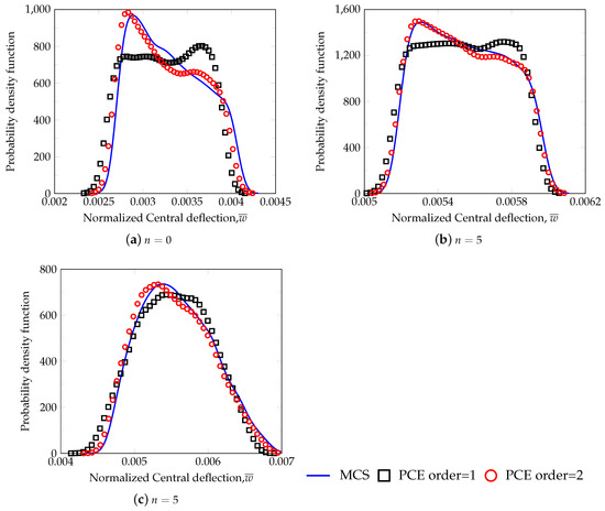
Figure 3.
Variation of the probability density function as a function of normalized central deflection; assuming the Young’s modulus of ceramic as random and (a) 0, (b) 5 and (c) the Young’s modulus of both metal and ceramic as random with .
Table 5.
Comparison of the mean and the standard deviation of the normalised central deflection for different cases between the Monte Carlo simulation (MCS) and the polynomial chaos expansion (PCE), considering PCE of order 1.
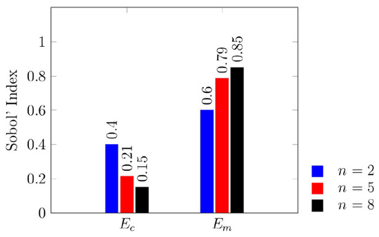
Figure 4.
Sensitivity study using the first order Sobol’ Indices for where the Young’s modulus of the both the ceramic and plate are the input random variables.
5.3. Free Vibration Analysis
The influence of randomness in material properties on the first two fundamental frequencies was studied. The randomness in the Young’s modulus and density, for two different gradient indices, 0, 5 were studied, considering the following cases:
- Case A: is random.
- Case B: and is random.
- Case C: and is random.
- Case D: and is random.
Figure 5, Figure 6, Figure 7 and Figure 8 show the probability density function for the first two normalised fundamental frequencies for two different gradient indices, 0 and 5 for Cases A–D. Results from the present method with PCE orders 1 and 2 are compared with the results from Monte Carlo Simulations runs of 10,000, where a close agreement is achieved. The mean frequency is observed to decrease with increasing gradient index, which is attributed to the increased metallic fraction.
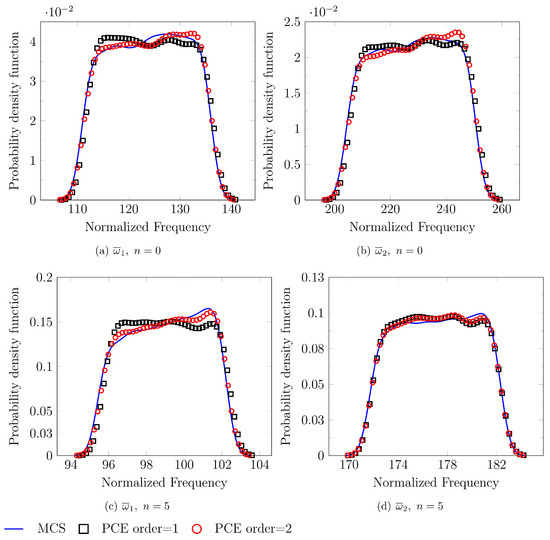
Figure 5.
Case A: Variation of the probability density function as a function of normalized frequency, for the first two normalised frequencies; considering gradient index, 0, 5 and the Young’s modulus of the ceramic as random.
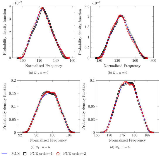
Figure 6.
Case B: Variation of the probability density function as a function of normalized frequency, for the first two normalised frequencies; considering gradient index, 0, 5 and the Young’s modulus and density of the ceramic as random.
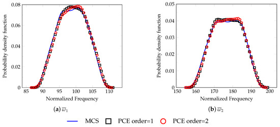
Figure 7.
Case C: Variation of the probability density function as a function of normalized frequency, for the first two normalised frequencies; considering gradient index, 5 and the Young’s modulus of both metal and ceramic as random.
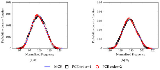
Figure 8.
Case D: Variation of the probability density function as a function of normalized frequency, for the first two normalised frequencies; considering gradient index, 5 and the Young’s modulus and density of both metal and ceramic as random.
When the number of random variables is four, the total number of evaluations performed using the PCE with Order 2 is 64, which is small when compared to 10,000 Monte Carlo simulations. The MCS took ≈45,062 s, whilst the PCE of order 2 took only around 189 s, which is much lower as compared to the former. In spite of this, it is observed from Figure 5, Figure 6, Figure 7 and Figure 8, that the proposed framework yields more accurate results. The mean and standard deviation of the first natural frequencies obtained from MCS and the PCE of order equal 1, are tabulated in Table 6. where the results from the PCE agrees well with the results from MCS.
Table 6.
Comparison of the mean and the standard deviation of the first two normalised natural frequencies for different cases between the MCS and the PCE. Here PCE order 1 is considered.
For each of the cases considered, the Sobol’ index is shown in Figure 9. For a homogeneous plate, i.e., 0, both the effective Young’s modulus and the density of the material have equal influence on the natural frequency of the plate. However, when , the effective Young’s modulus has a significant impact. When both metallic and ceramic Young’s modulus are considered to be random, the randomness in Young’s modulus of the metallic phase is noticed to have more influence on the normalised fundamental frequency. When all the material properties, Young’s modulus, and density of both the constituents are taken as random, density of the metallic phase has a significant influence on the output variable. These observations can be attributed to the increase in the metallic phase of the plate with an increasing gradient index. The influence of CoV of the metallic phase on the mean and standard deviation of the fundamental frequency is shown in Figure 10, where the influence of the gradient index is also depicted. It is inferred that the mean value of the fundamental frequency is found to be constant, and the standard deviation increases with increasing CoV.
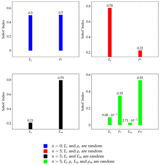
Figure 9.
Sensitivity study of the random parameters using the first order Sobol’ index for the first fundamental frequency of the functionally graded material plate.
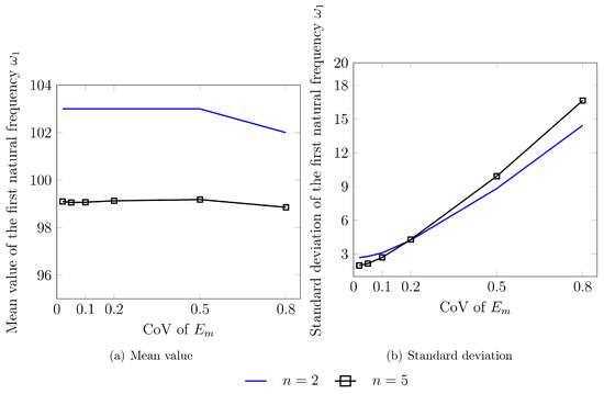
Figure 10.
(a) Mean and (b) standard deviation of the first natural frequency , for the variation of CoV of the metal, considering the gradient index n = 2 and 5.
6. Conclusions
In this study, the influence of randomness in the material properties of constituent materials on the static bending and free vibrations of FGM plates is studied using a non-intrusive approach. The stochastic response and its moments are obtained using the non-intrusive technique, with the help of PCE up to two orders. Results from the present analysis are compared with with 10,000 MCS realizations. A global sensitivity analysis is performed to determine the influence of the input randomness on the output variance, by computing the Sobol’ indices, which are determined directly from the PCE’s coefficients without any additional sampling. From the numerical analysis, it is inferred that the results estimated using the developed methodology, based on the polynomial chaos expansion of the output variables are found to be in close agreement with the results from Monte Carlo simulations. Therefore, the developed framework can thus be used for studying the influence of other parameters without having to carry out the computationally intensive Monte Carlo simulations. The salient features of the proposed framework are:
- It can handle a wider range of CoV, unlike the perturbation based methods.
- Does not require to modify the existing code like the intrusive based approaches.
Author Contributions
Data curation, S.M.D.; Formal analysis, S.M.D.; Investigation, S.M.D.; Methodology, T.M.V.; Project administration, S.M.D.; Software, T.M.V.; Supervision, P.R.B. and S.N.; Validation, S.M.D.; Visualization, S.N.; Writing—original draft, S.M.D. and T.M.V.; Writing—review and editing, T.M.V., P.R.B. and S.N. All authors have read and agreed to the published version of the manuscript.
Funding
This research received no external funding.
Conflicts of Interest
The authors declare no conflict of interest.
References
- Balaganesan, G.; Khan, V.C. Energy absorption of repaired composite laminates subjected to impact loading. Compos. Part B Eng. 2016, 98, 39–48. [Google Scholar] [CrossRef]
- Budarapu, P.; Kumar, S.; Prusty, B.G.; Paggi, M. Stress transfer through the interphase in curved-fiber pullout tests of nanocomposites. Compos. Part B Eng. 2019, 165, 417–434. [Google Scholar] [CrossRef]
- Budarapu, P.; Thakur, S.; Kumar, S.; Paggi, M. Micromechanics of engineered interphases in nacre-like composite structures. Mech. Adv. Mater. Struct. 2020, 1–16. [Google Scholar] [CrossRef]
- Jagtap, K.; Lal, A.; Singh, B. Stochastic nonlinear free vibration analysis of elastically supported functionally graded materials plate with system randomness in thermal environment. Compos. Struct. 2011, 93, 3185–3199. [Google Scholar] [CrossRef]
- Kitipornchai, S.; Yang, J.; Liew, K. Random vibration of the functionally graded laminates in thermal environments. Comput. Methods Appl. Mech. Eng. 2006, 195, 1075–1095. [Google Scholar] [CrossRef]
- Liu, W.K.; Belytschko, T.; Mani, A. Random field finite elements. Int. J. Num. Methods Eng. 1986, 23, 1831–1845. [Google Scholar] [CrossRef]
- Takada, T. Weighted integral method in stochastic finite element analysis. Probab. Eng. Mech. 1990, 5, 146–156. [Google Scholar] [CrossRef]
- Ghanem, R.G.; Spanos, P.D. Spectral Stochastic Finite Element Formulation for Reliability Analysis. J. Eng. Mech. 1991, 117, 2351–2372. [Google Scholar] [CrossRef]
- Kleiber, M.; Hien, T.D. The Stochastic Finite Element Method: Basic Perturbation Technique and Computer Implementation; Applied Stochastic Models and Data Analysis; Wiley: Chichester, UK, 1992; p. 297. [Google Scholar]
- Sudret, B.; Kiureghian, A.D. Stochastic Finite Element Methods and Reliability: A State-of-the-art Report; Report No. UCB/SEMM-2000/08; Department of Civil and Environmental Engineering, University of California: Berkeley, CA, USA, 2000. [Google Scholar]
- Chiba, R.; Sugano, Y. Stochastic analysis of a thermoelastic problem in functionally graded plates with uncertain material properties. Arch. Appl. Mech. 2007, 78, 749. [Google Scholar] [CrossRef]
- Shaker, A.; Abdelrahman, W.; Tawfik, M.; Sadek, E. Stochastic Finite element analysis of the free vibration of functionally graded material plates. Comput. Mech. 2008, 41, 707–714. [Google Scholar] [CrossRef]
- Li, K.; Wu, D.; Gao, W. Spectral stochastic isogeometric analysis for static response of FGM plate with material uncertainty. Thin-Walled Struct. 2018, 132, 504–521. [Google Scholar] [CrossRef]
- Kumar, R.; Mukhopadhyay, T.; Pandey, K.; Dey, S. Stochastic buckling analysis of sandwich plates: The importance of higher order modes. Int. J. Mech. Sci. 2019, 152, 630–643. [Google Scholar] [CrossRef]
- Thanh, C.L.; Tran, L.V.; Bui, T.Q.; Nguyen, H.X.; Abdel-Wahab, M. Isogeometric analysis for size-dependent nonlinear thermal stability of porous FG microplates. Compos. Struct. 2019, 221, 110838. [Google Scholar] [CrossRef]
- Wu, F.; Gao, Q.; Xu, X.M.; Zhong, W.X. A Modified Computational Scheme for the Stochastic Perturbation Finite Element Method. Latin Am. J. Solids Struct. 2015, 12, 2480–2505. [Google Scholar] [CrossRef]
- Kumaraian, M.L.; Rebbagondla, J.; Mathew, T.V.; Natarajan, S. Stochastic vibration analysis of functionally graded material paltes with material randomness using cell based smoothed discrete shear gap method. Int. J. Struct. Stabil. Dyn. 2019, 19, 1950037-1–1950037-20. [Google Scholar] [CrossRef]
- Minh, P.P.; Duc, N.D. The effect of cracks on the stability of the functionally graded plates with variable-thickness using HSDT and phase-field theory. Compos. Part B Eng. 2019, 175, 107086. [Google Scholar] [CrossRef]
- Sepahvand, K.; Marburg, S.; Hardtke, H.J. Stochastic free vibration of orthotropic plates using generalized polynomial chaos expansion. J. Sound Vibr. 2012, 331, 167–179. [Google Scholar] [CrossRef]
- Karsh, P.; Mukhopadhyay, T.; Chakraborty, S.; Naskar, S.; Dey, S. A hybrid stochastic sensitivity analysis for low-frequency vibration and low-velocity impact of functionally graded plates. Compos. Part B Eng. 2019, 176, 107221. [Google Scholar] [CrossRef]
- Tran, L.V.; Phung-Van, P.; Lee, J.; Wahab, M.A.; Nguyen-Xuan, H. Isogeometric analysis for nonlinear thermomechanical stability of functionally graded plates. Compos. Struct. 2016, 140, 655–667. [Google Scholar] [CrossRef]
- Lieu, Q.X.; Lee, J. Modeling and optimization of functionally graded plates under thermo-mechanical load using isogeometric analysis and adaptive hybrid evolutionary firefly algorithm. Compos. Struct. 2017, 179, 89–106. [Google Scholar] [CrossRef]
- Sundararajan, N.; Prakash, T.; Ganapathi, M. Nonlinear free flexural vibrations of functionally graded rectangular and skew plates under thermal environments. Finite Elem. Anal. Des. 2005, 42, 152–168. [Google Scholar] [CrossRef]
- Rajasekaran, S.; Murray, D. Incremental finite element matrices. ASCE J. Struct. Div. 1973, 99, 2423–2438. [Google Scholar]
- Cottrell, J.A.; Hughes, T.J.; Bazilevs, Y. Isogeometric Analysis: Toward Integration of CAD and FEA; John Wiley: Hoboken, NJ, USA, 2009. [Google Scholar]
- Nguyen, V.P.; Simpson, R.N.; Bordas, S.; Rabczuk, T. An introduction to Isogeometric Analysis with Matlab implementation: FEM and XFEM formulations. arXiv 2012, arXiv:1205.2129. [Google Scholar]
- Kikuchi, F.; Ishii, K. An improved 4-node quadrilateral plate bending element of the Reissne-Mindlin type. Comput. Mech. 1999, 23, 240–249. [Google Scholar] [CrossRef]
- Valizadeh, N.; Natarajan, S.; Gonzalez-Estrada, O.A.; Rabczuk, T.; Bui, T.Q.; Bordas, S.P. NURBS-based finite element analysis of functionally graded plates: Static bending, vibration, buckling and flutter. Compos. Struct. 2013, 99, 309–326. [Google Scholar] [CrossRef]
- Wiener, N. The homogeneous chaos. Am. J. Math. 1938, 60, 897–936. [Google Scholar] [CrossRef]
- Nguyen-Xuan, H.; Tran, L.V.; Thai, H.; Nguyen-Thoi, T. Analysis of functionally graded plates by an efficient finite element method with node-based strain smoothing. Thin Walled Struct. 2012, 54, 1–18. [Google Scholar] [CrossRef]
- Matsunaga, H. Free vibration and stability of functionally graded plates according to a 2D higher-order deformation theory. Compos. Struct. 2008, 82, 499–512. [Google Scholar] [CrossRef]
- Lee, Y.; Zhao, X.; Liew, K. Thermo-elastic analysis of functionally graded plates using the element free kp−Ritz method. Smart Mater. Struct. 2009, 18, 035007. [Google Scholar] [CrossRef]
- Zhao, X.; Lee, Y.; Liew, K. Free vibration analysis of functionally graded plates using the element free kp−Ritz method. J. Sound Vibr. 2009, 319, 918–939. [Google Scholar] [CrossRef]
- Nguyen-Xuan, H.; Tran, L.V.; Nguyen-Thoi, T.; Vu-Do, H. Analysis of functionally graded plates using an edge-based smoothed finite element method. Compos. Struct. 2011, 93, 3019–3039. [Google Scholar] [CrossRef]


© 2020 by the authors. Licensee MDPI, Basel, Switzerland. This article is an open access article distributed under the terms and conditions of the Creative Commons Attribution (CC BY) license (http://creativecommons.org/licenses/by/4.0/).