A General Inertial Projection-Type Algorithm for Solving Equilibrium Problem in Hilbert Spaces with Applications in Fixed-Point Problems

Abstract

A plethora of applications from mathematical programming, such as minimax, and mathematical programming, penalization, fixed point to mention a few can be framed as equilibrium problems. Most of the techniques for solving such problems involve iterative methods that is why, in this paper, we introduced a new extragradient-like method to solve equilibrium problems in real Hilbert spaces with a Lipschitz-type condition on a bifunction. The advantage of a method is a variable stepsize formula that is updated on each iteration based on the previous iterations. The method also operates without the previous information of the Lipschitz-type constants. The weak convergence of the method is established by taking mild conditions on a bifunction. For application, fixed-point theorems that involve strict pseudocontraction and results for pseudomonotone variational inequalities are studied. We have reported various numerical results to show the numerical behaviour of the proposed method and correlate it with existing ones.

1. Introduction

For a nonempty, closed and convex subset $\mathcal{K}$ of a real Hilbert space $\mathcal{E}$ and $f:\mathcal{E}\times \mathcal{E}\to \mathcal{R}$ is a bifunction with $f(p_1,p_1)=0$, for each $p_1\in \mathcal{K}.$ A equilibrium problem [1,2] for f on the set $\mathcal{K}$ is defined in the following way:

$$\mathrm{Find}{\wp }^{*}\in \mathcal{K}\mathrm{such}\mathrm{that}f({\wp }^{*},p_1)\ge 0,\forall p_1\in \mathcal{K}.$$

(1)

The problem (1) is very general, it includes many problems, such as fixed point problems, variational inequalities problems, the optimization problems, the Nash equilibrium of non-cooperative games, the complementarity problems, the saddle point problems, and the vector optimization problem (for further details see [1,3,4]). The equilibrium problem is also considered as the famous Ky Fan inequality [2]. This above-defined particular format of an equilibrium problem (1) is initiated by Muu and Oettli [5] in 1992 and further investigation on its theoretical properties studied by Blum and Oettli [1]. The construction of new optimization-based methods and the modification and extension of existing methods, as well as the examination of their convergence analysis, is an important research direction in equilibrium problem theory. Many methods have been developed over the last few years to numerically solve the equilibrium problems in both finite and infinite dimensional Hilbert spaces, i.e., the extragradient algorithms [6,7,8,9,10,11,12,13,14] subgradient algorithms [15,16,17,18,19,20,21] inertial methods [22,23,24,25], and others in [26,27,28,29,30,31,32,33,34].

In particular, a proximal method [35] is an efficient way to solve equilibrium problems that are equivalent to solving minimization problems on each step. This approach is also considered as the two-step extragradient-like method in [6], because of the early contribution of the Korpelevich [36] extragradient method to solve the saddle point problems. More precisely, Tran et al. introduced a method in [6], in which an iterative sequence $\{u_{n+1}\}$ was generated in the following manner:

$$\left\{\begin{array}{c}{u}_n\in \mathcal{K},\hfill \\ v_n=\underset{}{argmin}\{\xi f(u_n,y)+\frac{1}{2}\parallel u_n-y{\parallel }^2:y\in \mathcal{K}\},\hfill \\ u_{n+1}=\underset{}{argmin}\{\xi f(v_n,y)+\frac{1}{2}\parallel u_n-y{\parallel }^2:y\in \mathcal{K}\},\hfill \end{array}\right.$$

where $0<\xi <min\left\{\frac{1}{2k_1},\frac{1}{2k_2}\right\}$ and $k_1,k_2$ are Lipschitz constants. Moreover, $\underset{y\in \mathcal{K}}{argmin}f(x)$ is the value of x in set $\mathcal{K}$ for which $f(x)$ attains it’s minimum. The iterative sequence generated from the above-described method provides a weak convergent iterative sequence and in order to operate it, previous knowledge of the Lipschitz-like constants are required. These Lipschitz-type constants are normally unknown or hard to evaluate. In order to overcome this situation, Hieu et al. [12] introduced an extension of the method in [37] to solve the problems of equilibrium in the following manner: let ${\left[t\right]}_{+}:=max\{t,0\}$ and choose $u_0\in \mathcal{K},$ $\mu \in (0,1)$ with ${\xi }_0>0$, such that

$$\left\{\begin{array}{c}{v}_n=\underset{}{argmin}\{{\xi }_{n}f(u_n,y)+\frac{1}{2}\parallel u_n-y{\parallel }^2:y\in \mathcal{K}\},\hfill \\ u_{n+1}=\underset{}{argmin}\{{\xi }_{n}f(v_n,y)+\frac{1}{2}\parallel u_n-y{\parallel }^2:y\in \mathcal{K}\},\hfill \end{array}\right.$$

where the stepsize sequence $\{{\xi }_n\}$ is updated in the following way:

$${\xi }_{n+1}=min\left\{{\xi }_n,\frac{\mu (\parallel u_n-v_n{\parallel }^2+\parallel u_{n+1}-v_n{\parallel }^2)}{2{[f(u_n,u_{n+1})-f(u_n,v_n)-f(v_n,u_{n+1})]}_{+}}\right\}.$$

Recently, Vinh and Muu proposed an inertial iterative algorithm in [38] to solve a pseudomonotone equilibrium problem. The key contribution is an inertial factor in the method that used to enhance the convergence speed of the iterative sequence. The iterative sequence $\{u_n\}$ was defined in the following manner:

(i)

Choose $u_{-1},u_0\in \mathcal{K},$ $\theta \in [0,1),$ $0<\xi <min\{\frac{1}{2k_1},\frac{1}{2k_2}\}$ where a sequence $\{{\rho }_n\}\subset [0,+\infty )$ is satisfies the following conditions:

$$\sum _{n=0}^{+\infty }{\rho }_n<+\infty .$$

(2)

(ii)

Choose ${\theta }_n$ satisfying $0\le {\theta }_n\le \overline{{\theta }_n}$ and

$$\overline{{\theta }_n}=\left\{\begin{array}{cc}min\left\{\theta ,\frac{{\rho }_n}{\parallel u_n-u_{n-1}\parallel }\right\}\hfill & if{u}_n\ne u_{n-1},\hfill \\ \theta \hfill & else.\hfill \end{array}\right.$$

(3)

(iii)

Compute

$$\left\{\begin{array}{c}{\varrho }_n=u_n+{\theta }_n(u_n-u_{n-1}),\hfill \\ v_n=\underset{}{argmin}\{\xi f({\varrho }_n,y)+\frac{1}{2}\parallel {\varrho }_n-y{\parallel }^2:y\in \mathcal{K}\},\hfill \\ u_{n+1}=\underset{}{argmin}\{\xi f(v_n,y)+\frac{1}{2}\parallel {\varrho }_n-y{\parallel }^2:y\in \mathcal{K}\}.\hfill \end{array}\right.$$

Recently, another efficient inertial algorithm proposed by Hieu et al. in [39] as follows: let $u_{n-1},u_n,v_n\in \mathcal{K},$ $\theta \in [0,1),$ $0<\xi \le \frac{1}{2k_2+8k_1}$ and the sequence $\{u_n\}$ was defined in the following manner:

$$\left\{\begin{array}{c}{\varrho }_n=u_n+\theta (u_n-u_{n-1}),\hfill \\ u_{n+1}=\underset{}{argmin}\{\xi f(v_n,y)+\frac{1}{2}\parallel {\varrho }_n-y{\parallel }^2:y\in \mathcal{K}\},\hfill \\ {\varrho }_{n+1}=u_{n+1}+\theta (u_{n+1}-u_n),\hfill \\ v_{n+1}=\underset{}{argmin}\{\xi f(v_n,y)+\frac{1}{2}\parallel {\varrho }_{n+1}-y{\parallel }^2:y\in \mathcal{K}\}.\hfill \end{array}\right.$$

In this article, we concentrates on projection methods that are normally well-established and easy to execute due to their efficient numerical computation. Motivated by the works of [12,38], we formulate an inertial explicit subgradient extragradient method to solve the pseudomonotone equilibrium problem. These results can be seen as the modification of the methods appeared in [6,12,38,39]. Under certain mild conditions, a weak convergence theorem is proved regarding the iterative sequence of the algorithm. Moreover, experimental studies have documented that the designed method tends to be more efficient when compared to the existing methods that are presented in [38,39].

The remainder of the paper has been arranged, as follows: Section 2 contains the elementary results used in this paper. Section 3 contains our main algorithm and proves their convergence. Section 4 and Section 5 incorporate the applications of our main results. Section 6 carries out the numerical results that prove the computational effectiveness of our suggested method.

2. Preliminaries

   Assume that $h:\mathcal{K}\to \mathcal{R}$ be a convex function on a nonempty, closed and convex subset $\mathcal{K}$ of a real Hilbert space $\mathcal{E}$ and subdifferential of a function h at $p_1\in \mathcal{K}$ is defined by

$$\partial h(p_1)=\{p_3\in \mathcal{E}:h(p_2)-h(p_1)\ge ⟨p_3,p_2-p_1⟩,\forall p_2\in \mathcal{K}\}.$$

Assume that $\mathcal{K}$ be a nonempty, closed and convex subset of a real Hilbert space $\mathcal{E}$ and Normal cone of $\mathcal{K}$ at $p_1\in \mathcal{K}$ is defined by

$$N_{\mathcal{K}}(p_1)=\{p_3\in \mathcal{E}:⟨p_3,p_2-p_1⟩\le 0,\forall p_2\in \mathcal{K}\}.$$

A metric projection $P_{\mathcal{K}}(p_1)$ for $p_1\in \mathcal{E}$ onto a closed and convex subset $\mathcal{K}$ of $\mathcal{E}$ is defined by

$$P_{\mathcal{K}}(p_1)=\underset{}{argmin}\{\parallel p_2-p_1\parallel :p_2\in \mathcal{K}\}.$$

Now, consider the following definitions of monotonicity a bifunction (see for details [1,40]). Assume that $f:\mathcal{E}\times \mathcal{E}\to \mathcal{R}$ on $\mathcal{K}$ for $\gamma >0$ is said to be

(1)

γ-strongly monotone if

$$f(p_1,p_2)+f(p_2,p_1)\le -\gamma {\parallel p_1-p_2\parallel }^2,\forall p_1,p_2\in \mathcal{K};$$

(2)

monotone if

$$f(p_1,p_2)+f(p_2,p_1)\le 0,\forall p_1,p_2\in \mathcal{K};$$

(3)

γ-strongly pseudomonotone if

$$f(p_1,p_2)\ge 0⟹f(p_2,p_1)\le -\gamma {\parallel p_1-p_2\parallel }^2,\forall p_1,p_2\in \mathcal{K};$$

(4)

pseudomonotone if

$$f(p_1,p_2)\ge 0⟹f(p_2,p_1)\le 0,\forall p_1,p_2\in \mathcal{K}.$$

We have the following implications from the above definitions:

$$(1)⟹(2)⟹(4)\mathrm{and}(1)⟹(3)⟹(4).$$

In general, the converses are not true. Suppose that $f:\mathcal{E}\times \mathcal{E}\to \mathcal{R}$ satisfy the Lipschitz-type condition [41] on a set $\mathcal{K}$ if there exist two constants $k_1,k_2>0$, such that

$$f(p_1,p_2)+f(p_2,p_3)+k_1\parallel p_1-p_2{\parallel }^2+k_2{\parallel p_2-p_3\parallel }^2\ge f(p_1,p_3),\forall p_1,p_2,p_3\in \mathcal{K}.$$

Lemma 1

([42]). Suppose $\mathcal{K}$ be a nonempty, closed and convex subset of $\mathcal{E}$ and $P_{\mathcal{K}}:\mathcal{E}\to \mathcal{K}$ is metric projection from $\mathcal{E}$ onto $\mathcal{K}$.

(i)

Let $p_1\in \mathcal{K}$ and $p_2\in \mathcal{E},$ we have

$$\parallel p_1-P_{\mathcal{K}}(p_2){\parallel }^2+\parallel P_{\mathcal{K}}(p_2)-p_2{\parallel }^2\le {\parallel p_1-p_2\parallel }^2.$$

(ii)

$p_3=P_{\mathcal{K}}(p_1)$ if and only if

$$⟨p_1-p_3,p_2-p_3⟩\le 0,\forall p_2\in \mathcal{K}.$$

(iii)

For any $p_2\in \mathcal{K}$ and $p_1\in \mathcal{E}$

$$\parallel p_1-P_{\mathcal{K}}(p_1)\parallel \le \parallel p_1-p_2\parallel .$$

Lemma 2

([43,44]). Assume that $h:\mathcal{K}\to \mathcal{R}$ be a convex, lower semicontinuous and subdifferentiable function on $\mathcal{K},$ where $\mathcal{K}$ is a nonempty, convex and closed subset of a Hilbert space $\mathcal{E}.$ Subsequently, $p_1\in \mathcal{K}$ is minimizer of a function h if and only if $0\in \partial h(p_1)+N_{\mathcal{K}}(p_1),$ where $\partial h(p_1)$ and $N_{\mathcal{K}}(p_1)$ denotes the subdifferential of h at $p_1\in \mathcal{K}$ and the normal cone of $\mathcal{K}$ at $p_1$, respectively.

Lemma 3

([45]). Let $\{u_n\}$ be a sequence in $\mathcal{E}$ and $\mathcal{K}\subset \mathcal{E}$, such that the following conditions are satisfied:

(i)

for every $u\in \mathcal{K},$ the ${lim}_{n\to \infty }\parallel u_n-u\parallel$ exists;

(ii)

each sequentially weak cluster limit point of the sequence $\{u_n\}$ belongs to $\mathcal{K}$.

Then, $\{u_n\}$ weakly converge to some element in $\mathcal{K}.$

Lemma 4

([46]). Let $\{q_n\}$ and $\{p_n\}$ be sequences of non-negative real numbers satisfying $q_{n+1}\le q_n+p_n,$ for each $n\in \mathcal{N}.$ If $\sum p_n<\infty ,$ then ${lim}_{n\to \infty }{q}_n$ exists.

Lemma 5

([47]). For every $p_1,p_2\in \mathcal{E}$ and $\zeta \in \mathcal{R},$ then

$$\parallel \zeta p_1+(1-\zeta )p_2{\parallel }^2=\zeta \parallel p_1{\parallel }^2+(1-\zeta )\parallel p_2{\parallel }^2-\zeta (1-\zeta ){\parallel p_1-p_2\parallel }^2.$$

Suppose that bifunction f satisfies the following conditions:

(f1)

f is pseudomonotone on $\mathcal{K}$ and $f(p_2,p_2)=0,$ for every $p_2\in \mathcal{K}$;

(f2)

f satisfies the Lipschitz-type condition on $\mathcal{E}$ with constants $k_1>0$ and $k_2>0;$

(f3)

$\underset{n\to \infty }{lim\; sup}f(p_n,v)\le f(p^{*},v)$ for every $v\in \mathcal{K}$ and $\{p_n\}\subset \mathcal{K}$ satisfying $p_n\rightharpoonup p^{*}$;

(f4)

$f(p_1,.)$ needs to be convex and subdifferentiable on $\mathcal{E}$ for all $p_1\in \mathcal{E}.$

3. The Modified Extragradient Algorithm for the Problem (1) and Its Convergence Analysis

We provide a method consisting of two strongly convex minimization problems with an inertial term and an explicit stepsize formula that are being used to enhance the convergence rate of the iterative sequence and to make the algorithm independent of the Lipschitz constants. For the sake of simplicity in the presentation, we will use the notation ${\left[t\right]}_{+}=max\{0,t\}$ and follow the conventions $\frac{0}{0}=+\infty$ and $\frac{a}{0}=+\infty$ $(a\ne 0).$ The detailed method is provided below (Algorithm 1):

Algorithm 1 (Modified Extragradient Algorithm for the Problem (1))

Initialization: Choose $u_{-1},u_0\in \mathcal{K},$ $\mu \in (0,1),$ ${\beta }_n\in (0,1],$ $\theta \in [0,1)$ and $\{{\rho }_n\}\subset [0,+\infty )$ satisfying $$\sum _{n=0}^{+\infty }{\rho }_n<+\infty .$$ (4) Iterative steps: Choose ${\theta }_n$ satisfying $0\le {\theta }_n\le \overline{{\theta }_n}$ and $$\overline{{\theta }_n}=\left\{\begin{array}{ll}min\left\{\theta ,\frac{{\rho }_n}{\parallel u_n-u_{n-1}\parallel }\right\}\hfill & if{u}_n\ne u_{n-1},\hfill \\ \theta \hfill & else.\hfill \end{array}\right.$$ (5) Step 1: Compute $$v_n=\underset{y\in \mathcal{K}}{argmin}\{{\xi }_{n}f({\varrho }_n,y)+\frac{1}{2}\parallel {\varrho }_n-y{\parallel }^2\},$$ where ${\varrho }_n=u_n+{\theta }_n(u_n-u_{n-1}).$ If ${\varrho }_n=v_n$; STOP. Else, go to next step. Step 2: Compute $u_{n+1}=(1-{\beta }_n){\varrho }_n+{\beta }_n{z}_n,$ where $$z_n=\underset{y\in \mathcal{K}}{argmin}\{{\xi }_{n}f(v_n,y)+\frac{1}{2}\parallel {\varrho }_n-y{\parallel }^2\}.$$ Step 3: Update the stepsize in the following manner: $${\xi }_{n+1}=min\left\{{\xi }_n,\frac{\mu \parallel {\varrho }_n-v_n{\parallel }^2+\mu {\parallel z_n-v_n\parallel }^2}{2{[f({\varrho }_n,z_n)-f({\varrho }_n,v_n)-f(v_n,z_n)]}_{+}}\right\}.$$ Put $n:=n+1$ and return to Iterative steps.

Lemma 6.

The sequence $\{{\xi }_n\}$ is monotonically decreasing with a lower bound $min\left\{\frac{\mu }{2max\{k_1,k_2\}},{\xi }_0\right\}$ and it converges to $\xi >0.$

Proof. 

From the definition of sequence $\{{\xi }_n\}$ implies that sequence $\{{\xi }_n\}$ decreasing monotonically. It is given that f satisfy the Lipschitz-type condition with $k_1$ and $k_2$. Let $f({\varrho }_n,z_n)-f({\varrho }_n,v_n)-f(v_n,z_n)>0$, such that

$$\begin{array}{cc}\hfill \frac{\mu (\parallel {\varrho }_n-v_n{\parallel }^2+\parallel z_n-v_n{\parallel }^2)}{2[f({\varrho }_n,z_n)-f({\varrho }_n,v_n)-f(v_n,z_n)]}& \ge \frac{\mu (\parallel {\varrho }_n-v_n{\parallel }^2+\parallel z_n-v_n{\parallel }^2)}{2[k_1\parallel {\varrho }_n-v_n{\parallel }^2+k_2\parallel z_n-v_n{\parallel }^2]}\hfill \\ \hfill & \ge \frac{\mu }{2max\{k_1,k_2\}}.\hfill \end{array}$$

(6)

The above implies that $\{{\xi }_n\}$ has a lower bound $min\left\{\frac{\mu }{2max\{k_1,k_2\}},{\xi }_0\right\}.$ Moreover, there exists a fixed real number $\xi >0$, such that ${lim}_{n\to \infty }{\xi }_n=\xi .$□

Remark 1.

Because of the summability of ${\displaystyle \sum _{n=0}^{+\infty }{\rho }_n}$ and the expression (5) implies that

$$\sum _{n=1}^{\infty }{\theta }_n\parallel u_n-u_{n-1}\parallel \le \sum _{n=1}^{\infty }\overline{{\theta }_n}\parallel u_n-u_{n-1}\parallel \le \sum _{n=1}^{\infty }\theta \parallel u_n-u_{n-1}\parallel <\infty ,$$

(7)

that implies

$$\underset{n\to \infty }{lim}\theta \parallel u_n-u_{n-1}\parallel =0.$$

(8)

Lemma 7.

Suppose that $f:\mathcal{E}\times \mathcal{E}\to \mathcal{R}$ be a bifunction satisfies the conditions(f1)–(f4). For each ${\wp }^{*}\in EP(f,\mathcal{K})\ne \varnothing$, we have

$$\parallel z_n-{\wp }^{*}{\parallel }^2\le \parallel {\varrho }_n-{\wp }^{*}{\parallel }^2-\left(1-\frac{\mu {\xi }_n}{{\xi }_{n+1}}\right)\parallel {\varrho }_n-v_n{\parallel }^2-\left(1-\frac{\mu {\xi }_n}{{\xi }_{n+1}}\right){\parallel z_n-v_n\parallel }^2.$$

Proof. 

From the value of $z_n$, we have

$$0\in {\partial }_2\left\{{\xi }_{n}f(v_n,y)+\frac{1}{2}{\parallel {\varrho }_n-y\parallel }^2\right\}(z_n)+N_{\mathcal{K}}(z_n).$$

For some $\omega \in \partial f(v_n,z_n)$, there exists $\overline{\omega }\in N_{\mathcal{K}}(z_n)$, such that

$${\xi }_n\omega +z_n-{\varrho }_n+\overline{\omega }=0.$$

The above expression implies that

$$⟨{\varrho }_n-z_n,y-z_n⟩={\xi }_n⟨\omega ,y-z_n⟩+⟨\overline{\omega },y-z_n⟩,\forall y\in \mathcal{K}.$$

For given $\overline{\omega }\in N_{\mathcal{K}}(z_n)$, imply that $⟨\overline{\omega },y-z_n⟩\le 0,$∀$y\in \mathcal{K}.$ It provides that

$$⟨{\varrho }_n-z_n,y-z_n⟩\le {\xi }_n⟨\omega ,y-z_n⟩,\forall y\in \mathcal{K}.$$

(9)

From $\omega \in \partial f(v_n,z_n)$, we have

$$f(v_n,y)-f(v_n,z_n)\ge ⟨\omega ,y-z_n⟩,\forall y\in \mathcal{E}.$$

(10)

Combining expressions (9) and (10) we obtain

$${\xi }_{n}f(v_n,y)-{\xi }_{n}f(v_n,z_n)\ge ⟨{\varrho }_n-z_n,y-z_n⟩,\forall y\in \mathcal{K}.$$

(11)

By substituting $y={\wp }^{*}$ in (11), gives that

$${\xi }_{n}f(v_n,{\wp }^{*})-{\xi }_{n}f(v_n,z_n)\ge ⟨{\varrho }_n-z_n,{\wp }^{*}-z_n⟩.$$

(12)

Because $f({\wp }^{*},v_n)\ge 0$, then $f(v_n,{\wp }^{*})\le 0,$ provides that

$$⟨{\varrho }_n-z_n,z_n-{\wp }^{*}⟩\ge {\xi }_{n}f(v_n,z_n).$$

(13)

From the formula of ${\xi }_{n+1},$ we obtain

$$f({\varrho }_n,z_n)-f({\varrho }_n,v_n)-f(v_n,z_n)\le \frac{\mu \parallel {\varrho }_n-v_n{\parallel }^2+\mu {\parallel z_n-v_n\parallel }^2}{2{\xi }_{n+1}}$$

(14)

From the expressions (13) and (14), we have

$$\begin{array}{cc}\hfill ⟨{\varrho }_n-z_n,z_n-{\wp }^{*}⟩& \ge {\xi }_n\{f({\varrho }_n,z_n)-f({\varrho }_n,v_n)\}\hfill \\ \hfill & -\frac{\mu {\xi }_n}{2{\xi }_{n+1}}\parallel {\varrho }_n-v_n{\parallel }^2-\frac{\mu {\xi }_n}{2{\xi }_{n+1}}{\parallel z_n-v_n\parallel }^2.\hfill \end{array}$$

(15)

Similar to expression (11), the value of $v_n$ gives that

$${\xi }_{n}f({\varrho }_n,y)-{\xi }_{n}f({\varrho }_n,v_n)\ge ⟨{\varrho }_n-v_n,y-v_n⟩,\forall y\in \mathcal{K}.$$

(16)

By substituting $y=z_n$ in the above expression, we have

$${\xi }_n\left\{f({\varrho }_n,z_n)-f({\varrho }_n,v_n)\right\}\ge ⟨{\varrho }_n-v_n,z_n-v_n⟩.$$

(17)

Combining the expressions (15) and (17), we obtain

$$\begin{array}{cc}\hfill ⟨{\varrho }_n-z_n,z_n-{\wp }^{*}⟩& \ge ⟨{\varrho }_n-v_n,z_n-v_n⟩\hfill \\ \hfill & -\frac{\mu {\xi }_n}{2{\xi }_{n+1}}\parallel {\varrho }_n-v_n{\parallel }^2-\frac{\mu {\xi }_n}{2{\xi }_{n+1}}{\parallel z_n-v_n\parallel }^2.\hfill \end{array}$$

(18)

We have the given formulas:

$$-2⟨{\varrho }_n-z_n,z_n-{\wp }^{*}⟩=-\parallel {\varrho }_n-{\wp }^{*}{\parallel }^2+\parallel z_n-{\varrho }_n{\parallel }^2+{\parallel z_n-{\wp }^{*}\parallel }^2.$$

$$2⟨v_n-{\varrho }_n,v_n-z_n⟩=\parallel {\varrho }_n-v_n{\parallel }^2+\parallel z_n-v_n{\parallel }^2-{\parallel {\varrho }_n-z_n\parallel }^2.$$

The above expressions with (18), we have

$$\parallel z_n-{\wp }^{*}{\parallel }^2\le \parallel {\varrho }_n-{\wp }^{*}{\parallel }^2-\left(1-\frac{\mu {\xi }_n}{{\xi }_{n+1}}\right)\parallel {\varrho }_n-v_n{\parallel }^2-\left(1-\frac{\mu {\xi }_n}{{\xi }_{n+1}}\right){\parallel z_n-v_n\parallel }^2.$$

□

Theorem 1.

Assume that $f:\mathcal{E}\times \mathcal{E}\to \mathcal{R}$ be a bifunction satisfies the conditions(f1)–(f4) and ${\wp }^{*}$ belongs to solution set $EP(f,\mathcal{K}).$ Subsequently, the sequences $\{{\varrho }_n\},$ $\{v_n\},$ $\{z_n\}$ and $\{u_n\}$ generated through Algorithm 1 weakly converges to ${\wp }^{*}.$ In addition, ${lim}_{n\to \infty }{P}_{EP(f,\mathcal{K})}(u_n)={\wp }^{*}.$

Proof. 

By value of $u_{n+1}$ through Lemma 5, we obtain

$$\begin{array}{cc}\hfill \parallel u_{n+1}-{\wp }^{*}{\parallel }^2& =\parallel (1-{\beta }_n){\varrho }_n+{\beta }_n{z}_n-{\wp }^{*}{\parallel }^2\hfill \\ \hfill & =\parallel (1-{\beta }_n)({\varrho }_n-{\wp }^{*})+{\beta }_n(z_n-{\wp }^{*}){\parallel }^2\hfill \\ \hfill & =(1-{\beta }_n)\parallel {\varrho }_n-{\wp }^{*}{\parallel }^2+{\beta }_n\parallel z_n-{\wp }^{*}{\parallel }^2-{\beta }_n(1-{\beta }_n){\parallel {\varrho }_n-z_n\parallel }^2\hfill \\ \hfill & \le (1-{\beta }_n)\parallel {\varrho }_n-{\wp }^{*}{\parallel }^2+{\beta }_n{\parallel z_n-{\wp }^{*}\parallel }^2.\hfill \end{array}$$

(19)

By Lemma 7 and expression (19), we obtain

$$\begin{array}{cc}\hfill \parallel u_{n+1}-{\wp }^{*}{\parallel }^2& \le \parallel {\varrho }_n-{\wp }^{*}{\parallel }^2\hfill \\ \hfill & -{\beta }_n\left(1-\frac{\mu {\xi }_n}{{\xi }_{n+1}}\right)\parallel {\varrho }_n-v_n{\parallel }^2-{\beta }_n\left(1-\frac{\mu {\xi }_n}{{\xi }_{n+1}}\right){\parallel z_n-v_n\parallel }^2.\hfill \end{array}$$

(20)

Because ${\xi }_n\to \xi ,$ then there exists a fixed number $ϵ\in (0,1-\mu )$, such that

$$\underset{n\to \infty }{lim}\left(1-\frac{\mu {\xi }_n}{{\xi }_{n+1}}\right)=1-\mu >ϵ>0.$$

Subsequently, there exist a fixed real number $N_1\in \mathcal{N}$ such that

$$\left(1-\frac{\mu {\xi }_n}{{\xi }_{n+1}}\right)>ϵ>0,\forall n\ge N_1.$$

(21)

Combining the expressions (20) and (21), we obtain

$$\parallel u_{n+1}-{\wp }^{*}{\parallel }^2\le {\parallel {\varrho }_n-{\wp }^{*}\parallel }^2,\forall n\ge N_1.$$

(22)

By definition of the ${\varrho }_n$, we have

$$\begin{array}{c}\hfill \parallel {\varrho }_n-{\wp }^{*}\parallel =\parallel u_n+{\theta }_n(u_n-u_{n-1})-{\wp }^{*}\parallel \le \parallel u_n-{\wp }^{*}\parallel +{\theta }_n\parallel u_n-u_{n-1}\parallel .\end{array}$$

(23)

From the definition of ${\varrho }_n$ in Algorithm 1, we obtain

$$\begin{array}{cc}\hfill \parallel {\varrho }_n-{\wp }^{*}{\parallel }^2& =\parallel u_n+{\theta }_n(u_n-u_{n-1})-{\wp }^{*}{\parallel }^2\hfill \\ \hfill & =\parallel (1+{\theta }_n)(u_n-{\wp }^{*})-{\theta }_n(u_{n-1}-{\wp }^{*}){\parallel }^2\hfill \\ \hfill & =(1+{\theta }_n)\parallel u_n-{\wp }^{*}{\parallel }^2-{\theta }_n\parallel u_{n-1}-{\wp }^{*}{\parallel }^2+{\theta }_n(1+{\theta }_n){\parallel u_n-u_{n-1}\parallel }^2\hfill \end{array}$$

(24)

$$\begin{array}{cc}\hfill & \le (1+{\theta }_n)\parallel u_n-{\wp }^{*}{\parallel }^2-{\theta }_n\parallel u_{n-1}-{\wp }^{*}{\parallel }^2+2\theta {\parallel u_n-u_{n-1}\parallel }^2.\hfill \end{array}$$

(25)

The expression (22) can also be written as

$$\begin{array}{cc}\hfill \parallel u_{n+1}-{\wp }^{*}\parallel & \le \parallel u_n-{\wp }^{*}\parallel +\theta \parallel u_n-u_{n-1}\parallel ,\forall n\ge N_1.\hfill \end{array}$$

(26)

By using Lemma 4 with expressions (7) and (26), we have

$$\underset{n\to \infty }{lim}\parallel u_n-{\wp }^{*}\parallel =l,\mathrm{for}\mathrm{some}\mathrm{finite}l\ge 0.$$

(27)

The equality (8) implies that

$$\begin{array}{c}\hfill \underset{n\to \infty }{lim}\parallel u_n-u_{n-1}\parallel =0.\end{array}$$

(28)

By letting $n\to \infty$ in (24) implies that

$$\underset{n\to \infty }{lim}\parallel {\varrho }_n-{\wp }^{*}\parallel =l.$$

(29)

From the expression (20) and (25), we have

$$\begin{array}{cc}\hfill & \parallel u_{n+1}-{\wp }^{*}{\parallel }^2\hfill \\ \hfill & \le (1+{\theta }_n)\parallel u_n-{\wp }^{*}{\parallel }^2-{\theta }_n\parallel u_{n-1}-{\wp }^{*}{\parallel }^2+2\theta {\parallel u_n-u_{n-1}\parallel }^2\hfill \\ \hfill & -{\beta }_n\left(1-\frac{\mu {\xi }_n}{{\xi }_{n+1}}\right)\parallel {\varrho }_n-v_n{\parallel }^2-{\beta }_n\left(1-\frac{\mu {\xi }_n}{{\xi }_{n+1}}\right){\parallel z_n-v_n\parallel }^2,\hfill \end{array}$$

(30)

which further implies that (for $n\ge N_1$)

$$\begin{array}{cc}\hfill & ϵ\beta \parallel {\varrho }_n-v_n{\parallel }^2+ϵ\beta {\parallel v_n-z_n\parallel }^2\hfill \\ \hfill & \le \parallel u_n-{\wp }^{*}{\parallel }^2-\parallel u_{n+1}-{\wp }^{*}{\parallel }^2+{\theta }_n\left(\parallel u_n-{\wp }^{*}{\parallel }^2-{\parallel u_{n-1}-{\wp }^{*}\parallel }^2\right)+2\theta {\parallel u_n-u_{n-1}\parallel }^2.\hfill \end{array}$$

(31)

By letting $n\to \infty$ in (31), we obtain

$$\underset{n\to \infty }{lim}\parallel {\varrho }_n-v_n\parallel =\underset{n\to \infty }{lim}\parallel v_n-z_n\parallel =0.$$

(32)

By using the Cauchy inequality and expression (32), we obtain

$$\underset{n\to \infty }{lim}\parallel {\varrho }_n-z_n\parallel \le \underset{n\to \infty }{lim}\parallel {\varrho }_n-v_n\parallel +\underset{n\to \infty }{lim}\parallel z_n-v_n\parallel =0.$$

(33)

The expressions (29) and (32) imply that

$$\underset{n\to \infty }{lim}\parallel v_n-{\wp }^{*}\parallel =\underset{n\to \infty }{lim}\parallel z_n-{\wp }^{*}\parallel =l.$$

(34)

It follows from the expressions (27), (29) and (34) that the sequences $\{{\varrho }_n\},$ $\{u_n\},$ $\{v_n\}$ and $\{z_n\}$ are bounded. Now, we need to use Lemma 3, for this it is compulsory to show that any weak sequential limit points of $\{u_n\}$ lies in the set $EP(f,\mathcal{K}).$ Consider z to be a weak limit point of $\{u_n\}$ i.e., there is a $\{u_{n_k}\}$ of $\{u_n\}$ that is weakly converges to $z.$ Because $\parallel u_n-v_n\parallel \to 0$, then $\{v_{n_k}\}$ also weakly converge to z and so $z\in \mathcal{K}.$ Now, it is renaming to show that $z\in EP(f,\mathcal{K}).$ From relation (11), due to ${\xi }_{n+1}$ and (17), we have

$$\begin{array}{cc}\hfill {\xi }_{n_k}f(v_{n_k},y)& \ge {\xi }_{n_k}f(v_{n_k},z_{n_k})+⟨{\varrho }_{n_k}-z_{n_k},y-z_{n_k}⟩\hfill \\ \hfill & \ge {\xi }_{n_k}f({\varrho }_{n_k},z_{n_k})-{\xi }_{n_k}f({\varrho }_{n_k},v_{n_k})-\frac{\mu {\xi }_{n_k}}{2{\xi }_{n_k+1}}{\parallel {\varrho }_{n_k}-v_{n_k}\parallel }^2\hfill \\ \hfill & -\frac{\mu {\xi }_{n_k}}{2{\xi }_{n_k+1}}{\parallel v_{n_k}-z_{n_k}\parallel }^2+⟨{\varrho }_{n_k}-z_{n_k},y-z_{n_k}⟩\hfill \\ \hfill & \ge ⟨{\varrho }_{n_k}-v_{n_k},z_{n_k}-v_{n_k}⟩-\frac{\mu {\xi }_{n_k}}{2{\xi }_{n_k+1}}{\parallel {\varrho }_{n_k}-v_{n_k}\parallel }^2\hfill \\ \hfill & -\frac{\mu {\xi }_{n_k}}{2{\xi }_{n_k+1}}{\parallel v_{n_k}-z_{n_k}\parallel }^2+⟨{\varrho }_{n_k}-z_{n_k},y-z_{n_k}⟩,\hfill \end{array}$$

(35)

where $y\in \mathcal{K}.$ It follows from (28), (32), (33) and the boundedness of $\{u_n\}$ right hand side tend to zero. Due to ${\xi }_{n_k}>0,$ condition (f3) and $v_{n_k}\rightharpoonup z,$ implies

$$0\le \underset{k\to \infty }{lim\; sup}f(v_{n_k},y)\le f(z,y),\forall y\in \mathcal{K}.$$

(36)

Because $z\in \mathcal{K}$ imply that $f(z,y)\ge 0,\forall y\in \mathcal{K}.$ It is prove that $z\in EP(f,\mathcal{K}).$ By Lemma 3, provides that $\{{\varrho }_n\},$ $\{v_n\},$ $\{z_n\}$ and $\{u_n\}$ weakly converges to ${\wp }^{*}$ as $n\to \infty .$

Finally, to prove that ${lim}_{n\to \infty }{P}_{EP(f,\mathcal{K})}(u_n)={\wp }^{*}.$ Let $q_n:=P_{EP(f,\mathcal{K})}(u_n),$ $\forall n\in \mathcal{N}.$ For any ${\wp }^{*}\in EP(f,\mathcal{K})$, we have

$$\parallel q_n\parallel \le \parallel q_n-u_n\parallel +\parallel u_n\parallel \le \parallel {\wp }^{*}-u_n\parallel +\parallel u_n\parallel .$$

(37)

Clearly, the above implies that sequence $\{q_n\}$ is bounded. Next, we need to show that $\{q_n\}$ is a Cauchy sequence. By using Lemma 1(iii) and (23), we have

$$\parallel u_{n+1}-q_{n+1}\parallel \le \parallel u_{n+1}-q_n\parallel \le \parallel u_n-q_n\parallel +\theta \parallel u_n-u_{n-1}\parallel ,\forall n\ge N_1.$$

(38)

Thus, Lemma 4 provides the existence of ${lim}_{n\to \infty }\parallel u_n-q_n\parallel .$ Next, take (23) ∀$m>n\ge N_1,$ we have

$$\begin{array}{cc}\hfill \parallel q_n-u_m\parallel & \le \parallel q_n-u_{m-1}\parallel +\theta \parallel u_n-u_{n-1}\parallel \hfill \\ \hfill & \le \cdots \le \parallel q_n-u_n\parallel +\theta \sum _{k=n}^{m-1}\parallel u_n-u_{n-1}\parallel .\hfill \end{array}$$

(39)

Suppose that $q_m,q_n\in EP(f,\mathcal{K})$ for $m>n\ge N_1,$ through Lemma 1(i) and (39), we have

$$\begin{array}{cc}\hfill & \parallel q_n-q_m{\parallel }^2\hfill \\ \hfill & \le \parallel q_n-u_m{\parallel }^2-{\parallel q_m-u_m\parallel }^2\hfill \\ \hfill & \le \parallel q_n-u_n{\parallel }^2+{\left(\theta \sum _{k=n}^{m-1}\parallel u_n-u_{n-1}\parallel \right)}^2+2\theta \parallel q_n-u_n\parallel \sum _{k=n}^{m-1}\parallel u_n-u_{n-1}\parallel -\parallel q_m-u_m{\parallel }^2.\hfill \end{array}$$

(40)

The existence of ${lim}_{n\to \infty }\parallel u_n-q_n\parallel$ and the summability of the series ${\sum }_n\parallel u_n-u_{n-1}\parallel <+\infty ,$ imply ${lim}_{n\to \infty }\parallel q_n-q_m\parallel =0,$∀$m>n.$ As a result, $\{q_n\}$ is a Cauchy sequence and due the closeness of the set $EP(f,\mathcal{K})$ the sequence $\{q_n\}$ strongly converges to $q^{*}\in EP(f,\mathcal{K}).$ Next, remaining to show that $q^{*}={\wp }^{*}.$ From Lemma 1(ii) and ${\wp }^{*},q^{*}\in EP(f,\mathcal{K})$, we have

$$⟨u_n-q_n,{\wp }^{*}-q_n⟩\le 0.$$

(41)

Because of $q_n\to q^{*}$ and $u_n\rightharpoonup {\wp }^{*}$, we obtain

$$⟨{\wp }^{*}-q^{*},{\wp }^{*}-q^{*}⟩\le 0,$$

implies that ${\wp }^{*}=q^{*}={lim}_{n\to \infty }{P}_{EP(f,\mathcal{K})}(u_n).$□

4. Applications to Solve Fixed Point Problems

Now, consider the applications of our results that are discussed in Section 3 to solve fixed-point problems involving $\kappa$-strict pseudo-contraction. Let $T:\mathcal{K}\to \mathcal{K}$ be a mapping and the fixed point problem is formulated in the following manner:

$$\mathrm{Find}{\wp }^{*}\in \mathcal{K}\mathrm{such}\mathrm{as}T({\wp }^{*})={\wp }^{*}.$$

Let a mapping $T:\mathcal{K}\to \mathcal{K}$ is said to be

(i)

sequentially weakly continuous on $\mathcal{K}$ if

$$T(p_n)\rightharpoonup T(p)\mathrm{for}\mathrm{every}\mathrm{sequence}\mathrm{in}\mathcal{K}\mathrm{satisfying}{p}_n\rightharpoonup p(\mathrm{weakly}\mathrm{converges});$$

(ii)

κ-strict pseudo-contraction [48] on $\mathcal{K}$ if

$$\parallel T{p}_1-T{p}_2{\parallel }^2\le \parallel p_1-p_2{\parallel }^2+\kappa {\parallel (p_1-T{p}_1)-(p_2-T{p}_2)\parallel }^2,\forall p_1,p_2\in \mathcal{K};$$

(42)

that is equivalent to

$$⟨T{p}_1-T{p}_2,p_1-p_2⟩\le \parallel p_1-p_2{\parallel }^2-\frac{1-\kappa }{2}{\parallel (p_1-T{p}_1)-(p_2-T{p}_2)\parallel }^2,\forall p_1,p_2\in \mathcal{K}.$$

(43)

Note: if we define $f(p_1,p_2)=⟨p_1-T{p}_1,p_2-p_1⟩,\forall p_1,p_2\in \mathcal{K}.$ Then, the problem (1) convert into the fixed point problem with $2k_1=2k_2=\frac{3-2\kappa }{1-\kappa }.$ The value of $v_n$ in Algorithm 1 convert into followings:

$$\begin{array}{cc}\hfill v_n& =\underset{y\in \mathcal{K}}{argmin}\{{\xi }_{n}f({\varrho }_n,y)+\frac{1}{2}\parallel {\varrho }_n-y{\parallel }^2\}\hfill \\ \hfill & =\underset{y\in \mathcal{K}}{argmin}\{{\xi }_n⟨{\varrho }_n-T({\varrho }_n),y-{\varrho }_n⟩+\frac{1}{2}\parallel {\varrho }_n-y{\parallel }^2\}\hfill \\ \hfill & =\underset{y\in \mathcal{K}}{argmin}\{{\xi }_n⟨{\varrho }_n-T({\varrho }_n),y-{\varrho }_n⟩+\frac{1}{2}\parallel {\varrho }_n{-y\parallel }^2+\frac{{\xi }_n^2}{2}\parallel {\varrho }_n-T({\varrho }_n){\parallel }^2-\frac{{\xi }_n^2}{2}\parallel {\varrho }_n-T({\varrho }_n){\parallel }^2\}\hfill \\ \hfill & =\underset{y\in \mathcal{K}}{argmin}\{\frac{1}{2}\parallel y-{\varrho }_n+{\xi }_n({\varrho }_n-T({\varrho }_n)){\parallel }^2\}\hfill \\ \hfill & =P_{\mathcal{K}}\left[{\varrho }_n-{\xi }_n({\varrho }_n-T({\varrho }_n))\right]=P_{\mathcal{K}}\left[(1-{\xi }_n){\varrho }_n+{\xi }_{n}T({\varrho }_n)\right].\hfill \end{array}$$

(44)

In the similar way to the expression (44), we obtain

$$z_n=P_{\mathcal{K}}\left[{\varrho }_n-{\xi }_n(v_n-T(v_n))\right].$$

(45)

As a consequence of the results in Section 3, we have the following fixed point theorem:

Corollary 1.

Assume that $T:\mathcal{K}\to \mathcal{K}$ to be a weakly continuous and κ-strict pseudocontraction with $Fix(T)\ne \varnothing .$ The sequences ${\varrho }_n,$ $v_n,$ $z_n$ and $u_n$ be generated in the following way:

(i)

Choose $u_{-1},u_0\in \mathcal{K},$ $\mu \in (0,1),$ ${\beta }_n\in (0,1],$ $\theta \in [0,1)$ and $\{{\rho }_n\}\subset [0,+\infty )$ satisfies the following condition:

$$\sum _{n=0}^{+\infty }{\rho }_n<+\infty .$$

(46)

(ii)

Choose ${\theta }_n$ satisfies $0\le {\theta }_n\le \overline{{\theta }_n}$, such that

$$\overline{{\theta }_n}=\left\{\begin{array}{cc}min\left\{\theta ,\frac{{\rho }_n}{\parallel u_n-u_{n-1}\parallel }\right\}\hfill & if{u}_n\ne u_{n-1},\hfill \\ \theta \hfill & else.\hfill \end{array}\right.$$

(47)

(iii)

Compute $u_{n+1}=(1-{\beta }_n){\varrho }_n+{\beta }_n{z}_n$, where

$$\left\{\begin{array}{c}{\varrho }_n=u_n+{\theta }_n(u_n-u_{n-1}),\hfill \\ v_n=P_{\mathcal{K}}\left[{\varrho }_n-{\xi }_n({\varrho }_n-T({\varrho }_n))\right],\hfill \\ z_n=P_{\mathcal{K}}\left[{\varrho }_n-{\xi }_n(v_n-T(v_n))\right].\hfill \end{array}\right.$$

(48)

(iv)

Revised the stepsize ${\xi }_{n+1}$ in the following way:

$${\xi }_{n+1}=min\left\{{\xi }_n,\frac{\mu \parallel {\varrho }_n-v_n{\parallel }^2+\mu {\parallel z_n-v_n\parallel }^2}{2{\left[⟨({\varrho }_n-v_n)-(T({\varrho }_n)-T(v_n)),z_n-v_n⟩\right]}_{+}}\right\}$$

Subsequently, $\{{\varrho }_n\},$ $\{v_n\},$ $\{z_n\}$ and $\{u_n\}$ be the sequences converges weakly to ${\wp }^{*}\in Fix(T).$

5. Application to Solve Variational Inequality Problems

Now, consider the applications of our results that are discussed in Section 3 in order to solve variational inequality problems involving pseudomonotone and Lipschitz-type continuous operator. Let a operator $L:\mathcal{K}\to \mathcal{K}$ and the variational inequality problem is formulated as follows:

$$\mathrm{Find}{\wp }^{*}\in \mathcal{K}\mathrm{such}\mathrm{that}⟨L({\wp }^{*}),y-{\wp }^{*}⟩\ge 0,\forall y\in \mathcal{K}.$$

A mapping $L:\mathcal{E}\to \mathcal{E}$ is said to be

(i)

L-Lipschitz continuous on $\mathcal{K}$ if

$$\parallel L(p_1)-L(p_2)\parallel \le L\parallel p_1-p_2\parallel ,\forall p_1,p_2\in \mathcal{K};$$

(ii)

monotone on $\mathcal{K}$ if

$$⟨L(p_1)-L(p_2),p_1-p_2⟩\ge 0,\forall p_1,p_2\in \mathcal{K};$$

(iii)

pseudomonotone on $\mathcal{K}$ if

$$⟨L(p_1),p_2-p_1⟩\ge 0⟹⟨L(p_2),p_1-p_2⟩\le 0,\forall p_1,p_2\in \mathcal{K}.$$

Note: let $f(p_1,p_2):=⟨L(p_1),p_2-p_1⟩,$ $\forall p_1,p_2\in \mathcal{K}.$ Thus, problem (1) translates into the problem (VIP) with $L=2k_1=2k_2.$ From the value of $v_n,$ we have

$$\begin{array}{cc}\hfill v_n& =\underset{y\in \mathcal{K}}{argmin}\left\{{\xi }_{n}f({\varrho }_n,y)+\frac{1}{2}{\parallel {\varrho }_n-y\parallel }^2\right\}\hfill \\ \hfill & =\underset{y\in \mathcal{K}}{argmin}\left\{{\xi }_n⟨L({\varrho }_n),y-{\varrho }_n⟩+\frac{1}{2}\parallel {\varrho }_n{-y\parallel }^2+\frac{{\xi }_n^2}{2}\parallel L({\varrho }_n){\parallel }^2-\frac{{\xi }_n^2}{2}{\parallel L({\varrho }_n)\parallel }^2\right\}\hfill \\ \hfill & =\underset{y\in \mathcal{K}}{argmin}\left\{\frac{1}{2}{\parallel y-({\varrho }_n-{\xi }_{n}L({\varrho }_n))\parallel }^2\right\}\hfill \\ \hfill & =P_{\mathcal{K}}[{\varrho }_n-{\xi }_{n}L({\varrho }_n)].\hfill \end{array}$$

(49)

In similar way to the expression (49), we obtain

$$z_n=P_{\mathcal{K}}[{\varrho }_n-{\xi }_{n}L(v_n)].$$

Suppose that a mapping L satisfies the following conditions:

(L1)

L is monotone on $\mathcal{K}$ with $VI(L,\mathcal{K})\ne \varnothing$;

(L2)

L is L-Lipschitz continuous on $\mathcal{K}$ with $L>0$;

(L3)

L is pseudomonotone on $\mathcal{K}$ with $VI(L,\mathcal{K})\ne \varnothing$; and,

(L4)

$\underset{n\to \infty }{lim\; sup}⟨L(p_n),p-p_n⟩\le ⟨L(p),y-p⟩,$$\forall y\in \mathcal{K}$ and $\{p_n\}\subset \mathcal{K}$ satisfying $p_n\rightharpoonup p.$

Next, let L to be monotone and (L4) can be removed. The condition (L4) is used to defined $f(u,v)=⟨L(u),v-u⟩$ and satisfy the conditions (L4). The condition (f3) is required to show $z\in EP(f,\mathcal{K})$ see (36). The condition (L4) is required to show $z\in VI(L,\mathcal{K}).$ Further, to show that $z\in VI(L,\mathcal{K}).$ By letting the monotonicity of operator L, we have

$$⟨L(y),y-v_n⟩\ge ⟨L(v_n),y-v_n⟩,\forall y\in \mathcal{K}.$$

(50)

By letting $f(u,v)=⟨L(u),v-u⟩$ with expression (35), implies that

$$\underset{k\to \infty }{lim\; sup}⟨L(v_{n_k}),y-v_{n_k}⟩\ge 0,\forall y\in \mathcal{K}.$$

(51)

Combining (50) with (51), we deduce that

$$\underset{k\to \infty }{lim\; sup}⟨L(y),y-v_{n_k}⟩\ge 0,\forall y\in \mathcal{K}.$$

(52)

Therefore, $v_{n_k}\rightharpoonup z\in \mathcal{K},$ provides $⟨L(y),y-z⟩\ge 0,$∀$y\in \mathcal{K}.$ Let $v_t=(1-t)z+ty,$∀$t\in [0,1].$ Since $v_t\in \mathcal{K}$ for $t\in (0,1)$, we have

$$0\le ⟨L(v_t),v_t-z⟩=t⟨L(v_t),y-z⟩.$$

(53)

That is $⟨L(v_t),y-z⟩\ge 0$ every $t\in (0,1).$ Due to $v_t\to z$, while $t\to 0$, we have $⟨L(z),y-z⟩\ge 0,$ for all $y\in \mathcal{K},$ consequently $z\in VI(L,\mathcal{K}).$

Corollary 2.

Let $L:\mathcal{K}\to \mathcal{E}$ be a mapping and satisfying the conditions(L1)–(L2). Assume that the sequences $\{{\varrho }_n\},$ $\{v_n\},$ $\{z_n\}$ and $\{u_n\}$ generated in the following manner:

(i)

Choose $u_{-1},u_0\in \mathcal{K},$ $\mu \in (0,1),$ ${\beta }_n\in (0,1],$ $\theta \in [0,1)$ and $\{{\rho }_n\}\subset [0,+\infty )$, such that

$$\sum _{n=0}^{+\infty }{\rho }_n<+\infty .$$

(54)

(ii)

Let ${\theta }_n$ satisfies $0\le {\theta }_n\le \overline{{\theta }_n}$ and

$$\overline{{\theta }_n}=\left\{\begin{array}{cc}min\left\{\theta ,\frac{{\rho }_n}{\parallel u_n-u_{n-1}\parallel }\right\}\hfill & if{u}_n\ne u_{n-1},\hfill \\ \theta \hfill & otherwise.\hfill \end{array}\right.$$

(55)

(iii)

Compute $u_{n+1}=(1-{\beta }_n){\varrho }_n+{\beta }_n{z}_n,$ where

$$\left\{\begin{array}{c}{\varrho }_n=u_n+{\theta }_n(u_n-u_{n-1}),\hfill \\ v_n=P_{\mathcal{K}}[{\varrho }_n-{\xi }_{n}L({\varrho }_n)],\hfill \\ z_n=P_{\mathcal{K}}[{\varrho }_n-{\xi }_{n}L(v_n)].\hfill \end{array}\right.$$

(56)

(iv)

Stepsize ${\xi }_{n+1}$ is revised in the following way:

$${\xi }_{n+1}=min\left\{{\xi }_n,\frac{\mu \parallel {\varrho }_n-v_n{\parallel }^2+\mu {\parallel z_n-v_n\parallel }^2}{2{\left[⟨L({\varrho }_n)-L(v_n),z_n-v_n⟩\right]}_{+}}\right\}$$

Subsequently, the sequences $\{{\varrho }_n\},$ $\{v_n\},$ $\{z_n\}$ and $\{z_n\}$ converge weakly to ${\wp }^{*}\in VI(L,\mathcal{K}).$

Corollary 3.

Let $L:\mathcal{K}\to \mathcal{E}$ be a mapping and satisfying the conditions(L2)–(L4). Assume that the sequences $\{{\varrho }_n\},$ $\{v_n\},$ $\{z_n\}$ and $\{u_n\}$ generated in the following manner:

(i)

Choose $u_{-1},u_0\in \mathcal{K},$ $\mu \in (0,1),$ ${\beta }_n\in (0,1],$ $\theta \in [0,1)$ and $\{{\rho }_n\}\subset [0,+\infty )$, such that

$$\sum _{n=0}^{+\infty }{\rho }_n<+\infty .$$

(57)

(ii)

Choose ${\theta }_n$ satisfying $0\le {\theta }_n\le \overline{{\theta }_n}$, such that

$$\overline{{\theta }_n}=\left\{\begin{array}{cc}min\left\{\theta ,\frac{{\rho }_n}{\parallel u_n-u_{n-1}\parallel }\right\}\hfill & if{u}_n\ne u_{n-1},\hfill \\ \theta \hfill & else.\hfill \end{array}\right.$$

(58)

(iii)

Compute $u_{n+1}=(1-{\beta }_n){\varrho }_n+{\beta }_n{z}_n,$ where

$$\left\{\begin{array}{c}{\varrho }_n=u_n+{\theta }_n(u_n-u_{n-1}),\hfill \\ v_n=P_{\mathcal{K}}[{\varrho }_n-{\xi }_{n}L({\varrho }_n)],\hfill \\ z_n=P_{\mathcal{K}}[{\varrho }_n-{\xi }_{n}L(v_n)].\hfill \end{array}\right.$$

(59)

(iv)

The stepsize ${\xi }_{n+1}$ is updated in the following way:

$${\xi }_{n+1}=min\left\{{\xi }_n,\frac{\mu \parallel {\varrho }_n-v_n{\parallel }^2+\mu {\parallel z_n-v_n\parallel }^2}{2{\left[⟨L({\varrho }_n)-L(v_n),z_n-v_n⟩\right]}_{+}}\right\}$$

Subsequently, the sequences $\{{\varrho }_n\},$ $\{v_n\},$ $\{z_n\}$ and $\{z_n\}$ converge weakly to ${\wp }^{*}\in VI(L,\mathcal{K}).$

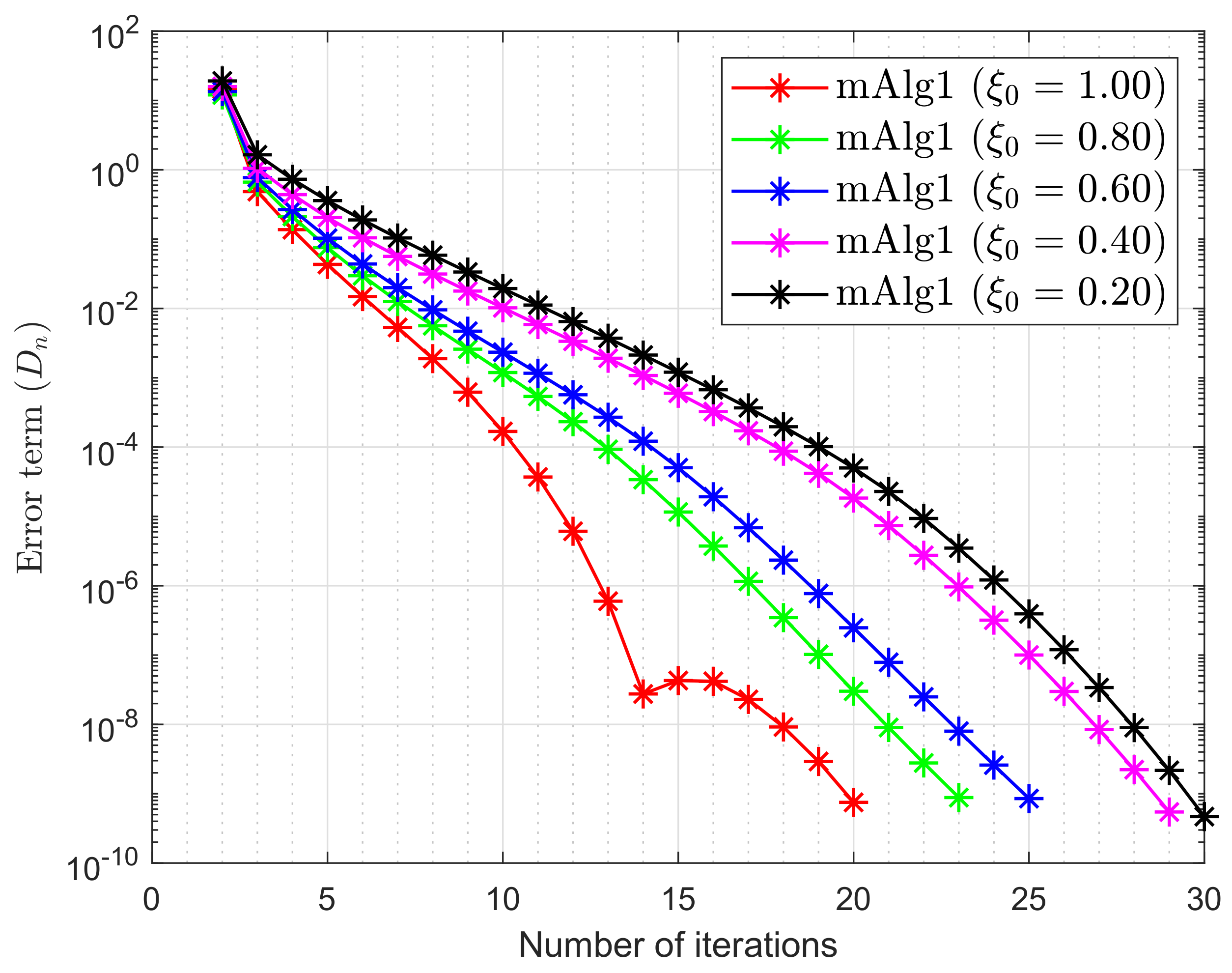
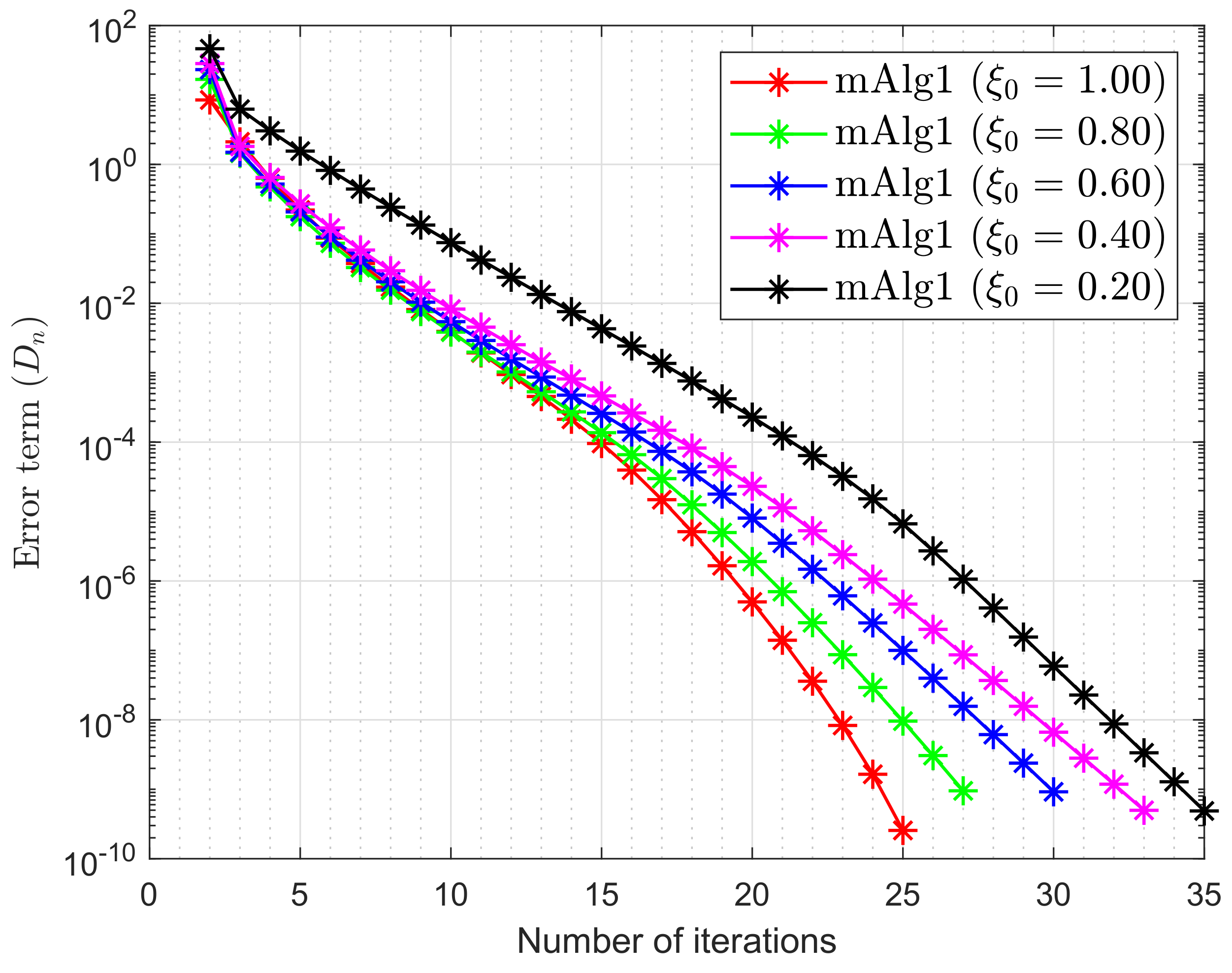
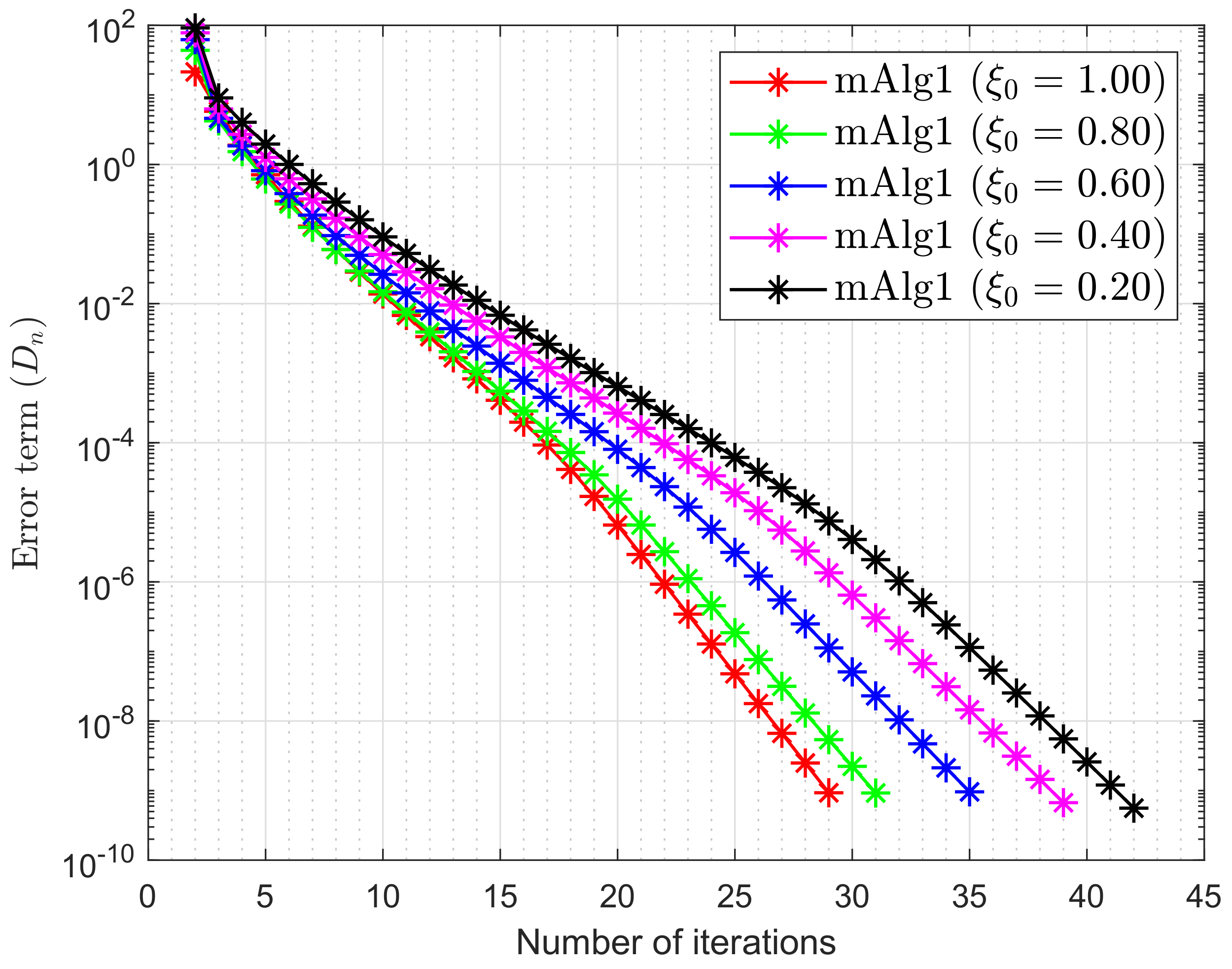
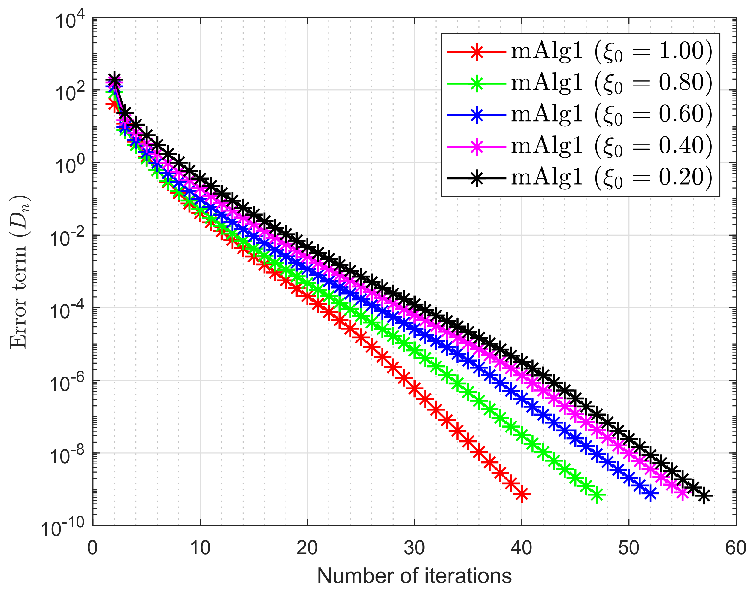
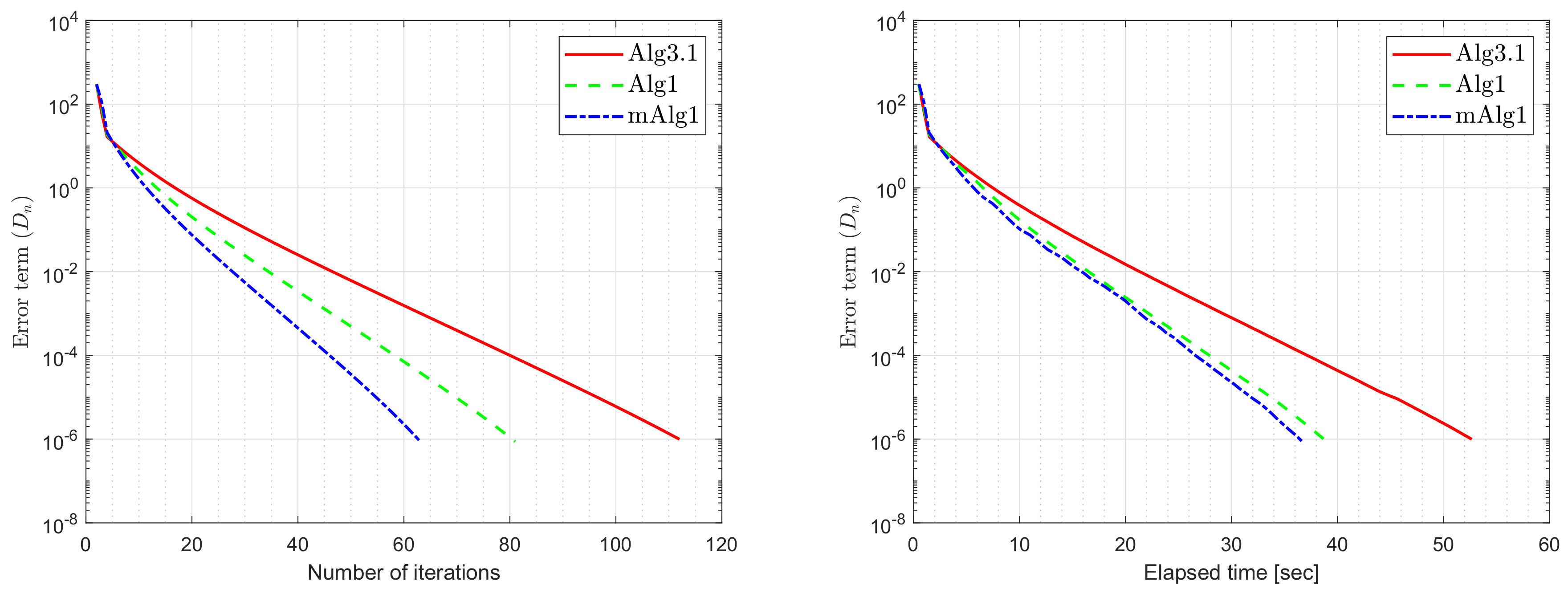
6. Numerical Experiments

The computational results present this section to prove the effectiveness of Algorithm 1 when compared to Algorithm 3.1 in [39] and Algorithm 1 in [38].

(i)

For Algorithm 3.1 (Alg3.1) in [39]:

$$\xi =\frac{1}{10max\{k_1,k_2\}},\theta =\frac{1}{2},\mathrm{Error}\mathrm{term}(D_n)=max\{\parallel u_{n+1}-v_n{\parallel }^2,\parallel u_{n+1}-{\varrho }_n{\parallel }^2\}.$$

(ii)

For Algorithm 1 (Alg1) in [38]:

$$\xi =\frac{1}{4max\{k_1,k_2\}},\theta =\frac{1}{2},{\rho }_n=\frac{1}{n^2},\mathrm{Error}\mathrm{term}(D_n)={\parallel {\varrho }_n-v_n\parallel }^2.$$

(iii)

For Algorithm 1 (mAlg1):

$$\xi =\frac{1}{2},\theta =\frac{1}{2},\mu =\frac{1}{3},{\rho }_n=\frac{1}{n^2},{\beta }_n=\frac{8}{10},\mathrm{Error}\mathrm{term}(D_n)={\parallel {\varrho }_n-v_n\parallel }^2.$$

Example 1.

Let take the Nash–Cournot Equilibrium Model that found in the paper [6]. A bifunction f consider into the following form:

$$f(p_1,p_2)=⟨P{p}_1+Q{p}_2+q,p_2-p_1⟩,$$

where $q\in {\mathcal{R}}^m$ with matrices P, Q of order m and Lipschitz constants are $k_1=k_2=\frac{1}{2}\parallel P-Q\parallel$ (see for more details [6]). In our case, $P,Q$ are taken at random (choose diagonal matrices $A_1$ and $A_2$ randomly entries from $[0,2]$ and $[-2,0]$, respectively. Two random orthogonal matrices $B_1$ and $B_2$ provide positive semidefinite matrix $M_1=B_1{A}_1{B}_1^T$ and negative semidefinite matrix $M_2=B_2{A}_2{B}_2^T.$ Finally, set $Q=M_1+M_1^T,$ $S=M_2+M_2^T$ and $P=Q-S.$) and elements of q are taken arbitrary form $[-1,1].$ A set $\mathcal{K}\subset {\mathcal{R}}^m$ is taken as

$$\mathcal{K}:=\{u\in {\mathcal{R}}^m:-10\le u_i\le 10\}.$$

Table 1 and Table 2 and Figure 1, Figure 2, Figure 3, Figure 4, Figure 5, Figure 6, Figure 7 and Figure 8 presented the numerical results by taking $u_{-1}=u_0=v_0=(1,\cdots ,1)$ and $D_n\le {10}^{-9}.$

Table 1. Example 1: Algorithm 1 numerical behaviour by letting different options for ${\xi }_0$ and m.

	m = 10		m = 20		m = 50		m = 100
${\mathbf{\xi }}_{\mathbf{0}}$	iter.	time	iter.	time	iter.	time	iter.	time
1.00	20	0.1701	25	0.2153	29	0.2726	40	0.5570
0.80	23	0.1945	27	0.2326	31	0.2788	47	0.5469
0.60	25	0.1995	30	0.2634	35	0.3285	52	0.6228
0.40	29	0.1467	33	0.2979	39	0.3549	55	0.6542
0.20	30	0.2632	35	0.2868	42	0.3849	57	0.6662

Table 2. Example 1: Algorithm 1 (mAlg1) numerical comparison with Algorithm 3.1 (Alg3.1) in [39] and Algorithm 1 (Alg1) in [38].

	Number of Iterations			Execution Time in Seconds
$\mathit{m}$	Alg3.1	Alg1	mAlg1	Alg3.1	Alg1	mAlg1
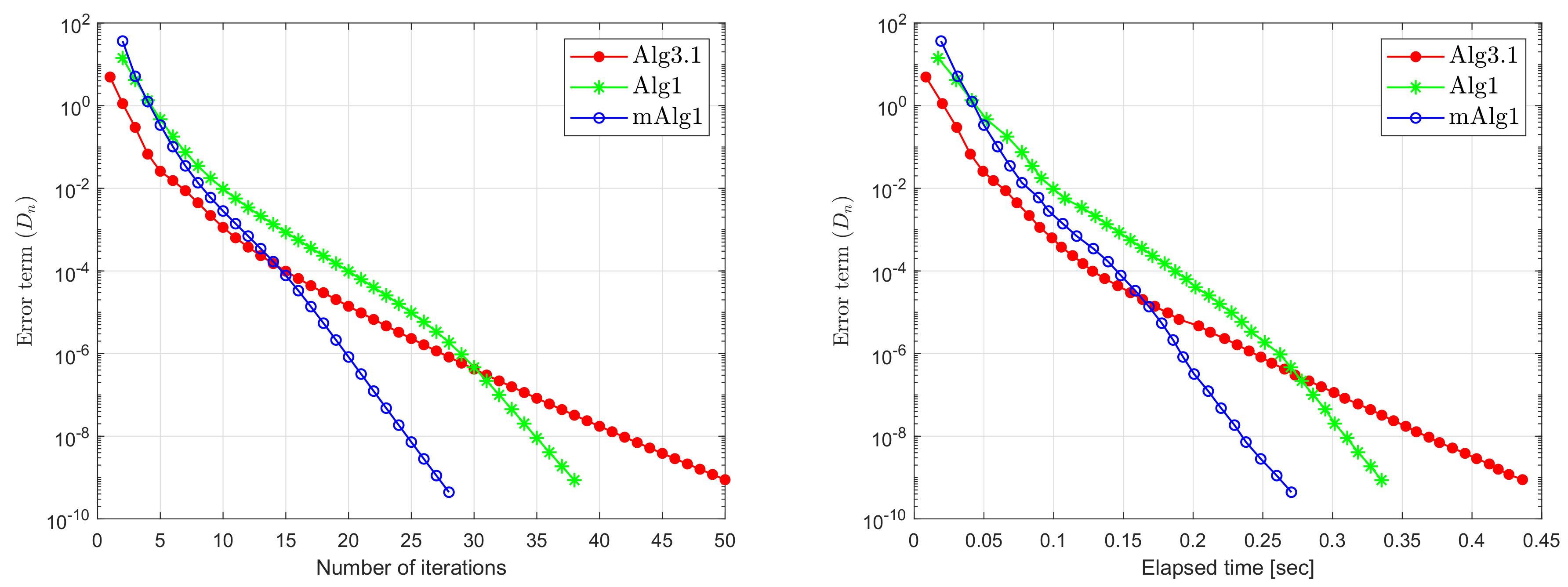
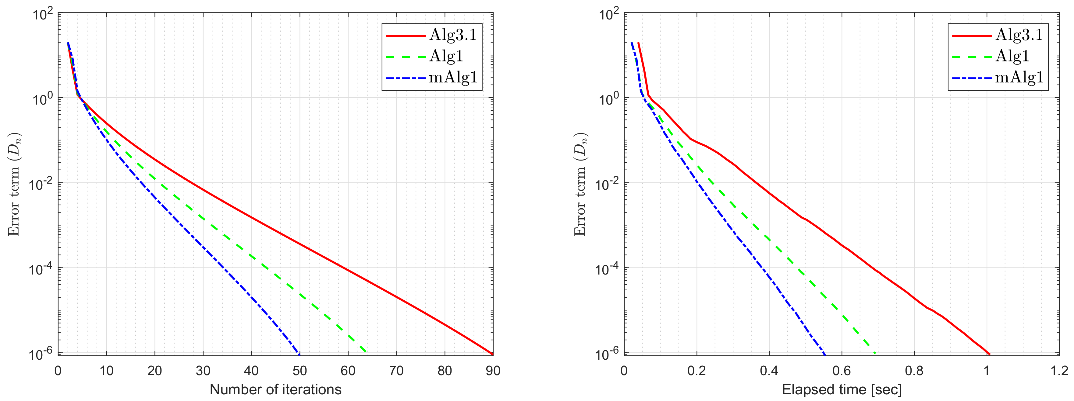
60	50	38	28	0.4362	0.3352	0.2705
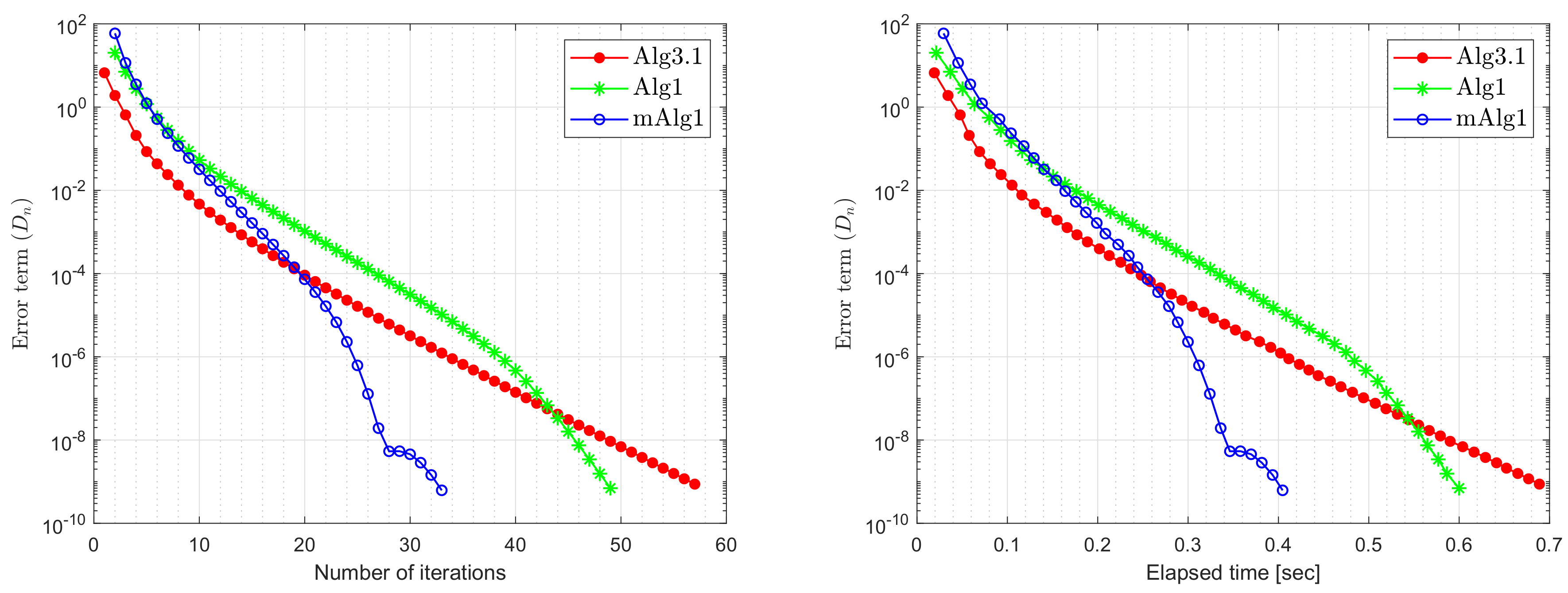
120	57	49	33	0.6888	0.6000	0.4047
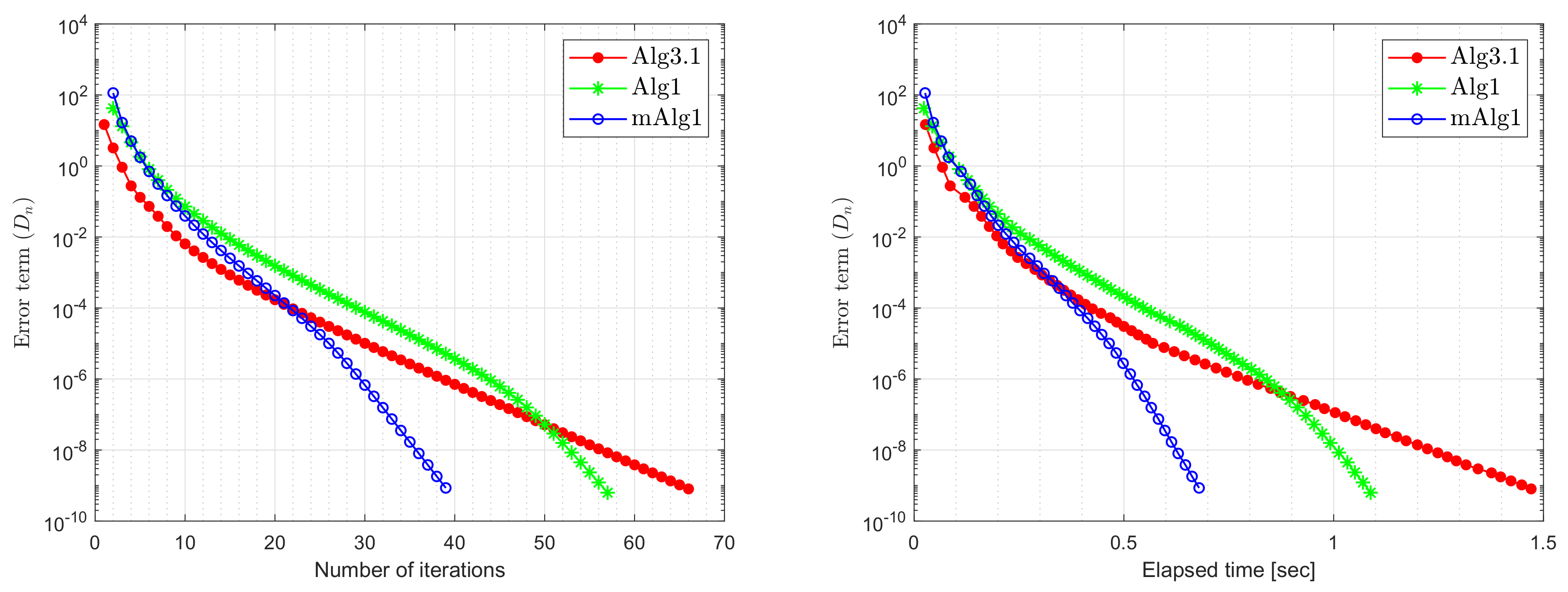
200	66	57	39	1.4708	1.0881	0.6794
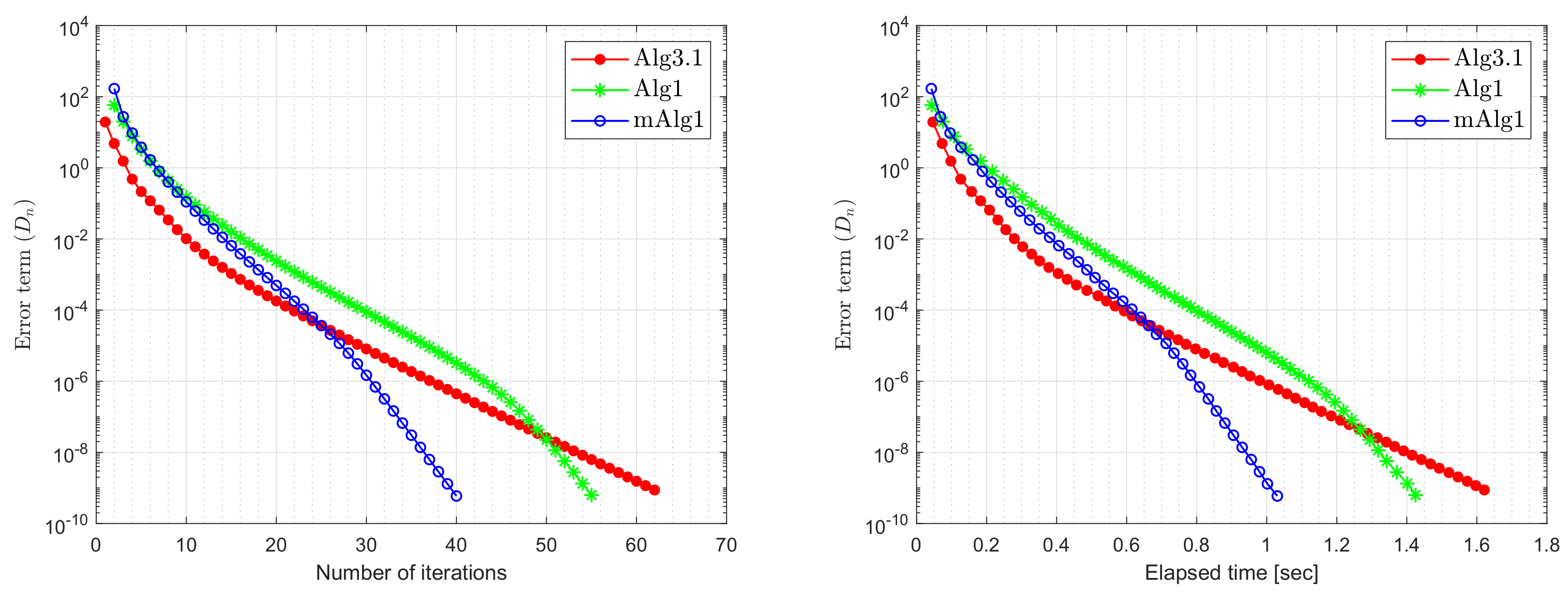
300	62	55	40	1.6213	1.4251	1.0303

Figure 1. Example 1: numerical behaviour of Algorithm 1 by letting different options for ${\xi }_0$, while m = 10.

Figure 2. Example 1: numerical behaviour of Algorithm 1 by letting different options for ${\xi }_0$, while m = 20.

Figure 3. Example 1: numerical behaviour of Algorithm 1 by letting different options for ${\xi }_0$ while m = 50.

Figure 4. Example 1: numerical behaviour of Algorithm 1 by letting different options for ${\xi }_0$ while m = 100.

Figure 5. Example 1: Algorithm 1 (mAlg1) numerical comparison with Algorithm 3.1 (Alg3.1) in [39] and Algorithm 1 (Alg1) in [38] while m = 60.

Figure 6. Example 1: Algorithm 1 (mAlg1) numerical comparison with Algorithm 3.1 (Alg3.1) in [39] and Algorithm 1 (Alg1) in [38] while m = 120.

Figure 7. Example 1: Algorithm 1 (mAlg1) numerical comparison with Algorithm 3.1 (Alg3.1) in [39] and Algorithm 1 (Alg1) in [38] while m = 200.

Figure 8. Example 1: Algorithm 1 (mAlg1) numerical comparison with Algorithm 3.1 (Alg3.1) in [39] and Algorithm 1 (Alg1) in [38] while m = 300.

Example 2.

Suppose that $f:\mathcal{K}\times \mathcal{K}\to \mathcal{R}$ be a bifunction defined in the following way

$$f(p,q)=\sum _{i=2}^5(q_i-p_i)\parallel p\parallel ,\forall p,q\in {\mathcal{R}}^5,$$

where $\mathcal{K}=\left\{(p_1,\cdots ,p_5):p_1\ge -1,p_i\ge 1,i=2,\cdots ,5\right\}.$ A bifunction f is Lipschitz-type continuous with constants $k_1=k_2=2$ and satisfy the conditions(f1)–(f4). In order to evaluate the best possible value of the control parameters, a numerical test is performed taking the variation of the inertial factor $\theta .$ The numerical comparison results are shown in the Table 3 by using $u_{-1}=u_0=v_0=(2,3,2,5,5)$ and $D_n\le {10}^{-6}.$

Table 3. Example 2: Algorithm 1 (mAlg1) numerical comparison with Algorithm 3.1 (Alg3.1) in [39] and Algorithm 1 (Alg1) in [38].

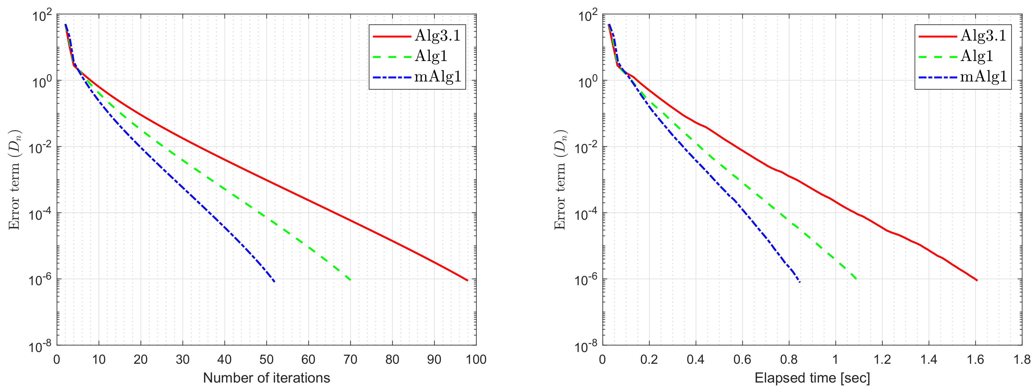
	Number of Iterations			Execution Time in Seconds
$\mathbf{\theta }$	Alg3.1	Alg1	mAlg1	Alg3.1	Alg1	mAlg1
0.90	67	56	47	2.8674	2.5324	1.6734
0.70	63	53	45	2.7813	2.6423	1.5026
0.50	57	47	41	2.0912	2.4212	1.4991
0.30	61	48	44	2.4115	2.3567	1.5092
0.10	69	60	47	2.9229	2.2881	1.5098

Example 3.

Let $\mathcal{E}=L^2([0,1])$ be a Hilbert space with an inner product $⟨p,q⟩={\int }_0^{1}p(r)q(r)dr,$ and the induced norm $\parallel p\parallel =\sqrt{{\int }_0^1{p}^2(r)dr},$ $\forall p,q\in \mathcal{E}.$ The set $\mathcal{K}:=\{p\in L^2([0,1]):{\int }_0^{1}rp(r)dr=2\}.$ Suppose that $f:\mathcal{E}\times \mathcal{E}\to \mathcal{R}$ is defined by

$$f(p,q)=⟨L(p),q-p⟩,$$

where $L(p(r))={\int }_0^{r}p(s)ds,$ for every $p\in L^2([0,1])$ and $r\in [0,1].$ The projection on set $\mathcal{K}$ is computed in the following way:

$$P_{\mathcal{K}}(p)(r):=p(r)-\frac{{\int }_0^{1}rp(r)dr-2}{{\int }_0^1{r}^{2}dr}r,r\in [0,1].$$

Table 4 reports the numerical results by using stopping criterion $D_n\le {10}^{-6}$ and letting $u_{-1}=u_0=v_0.$

Table 4. Example 3: Algorithm 1 (mAlg1) numerical comparison with Algorithm 3.1 (Alg3.1) in [39] and Algorithm 1 (Alg1) in [38].

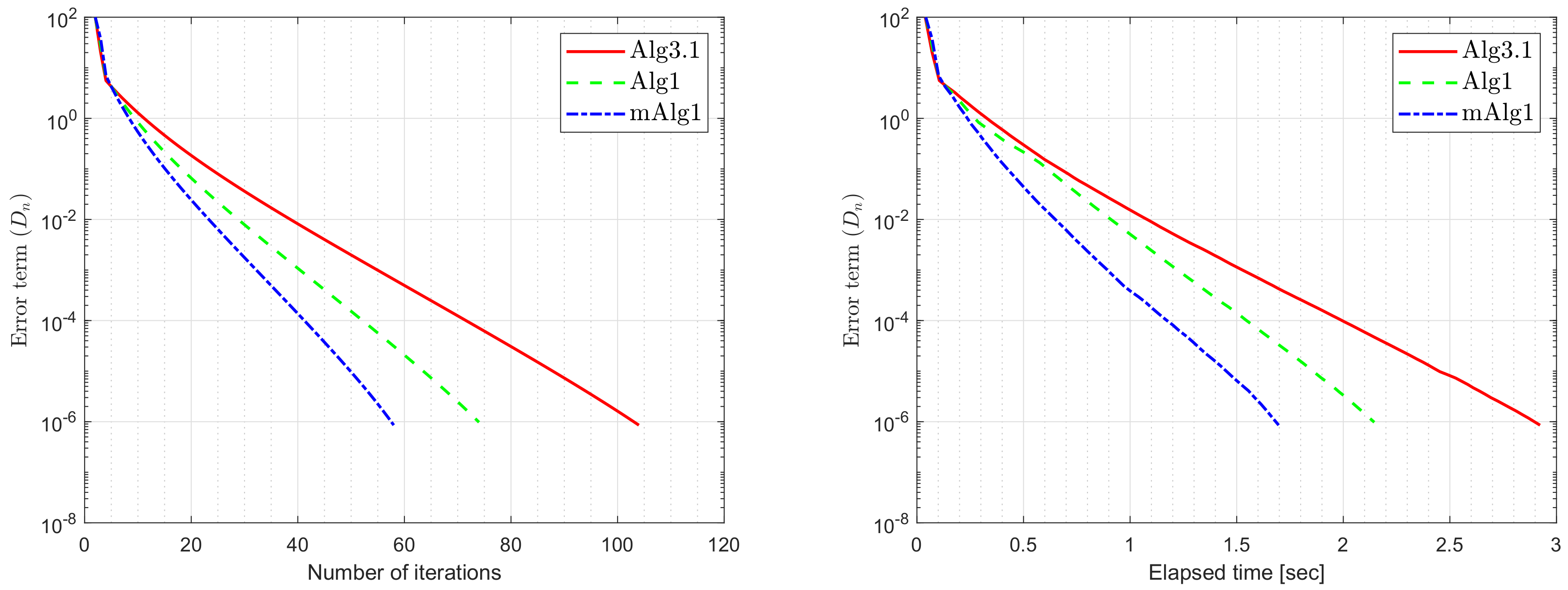
	Number of Iterations			Execution time in Seconds
${\mathit{u}}_{\mathbf{0}}$	Alg3.1	Alg1	mAlg1	Alg3.1	Alg1	mAlg1
$3t$	33	28	19	4.7654	3.9782	2.9342
$3t^2$	38	31	20	5.2598	4.1458	3.0987
$3sin(t)$	41	33	22	5.9876	5.3976	4.4298
$3cos(t)$	47	39	22	6.9921	5.4765	4.4611
$3exp{(t)}^2$	58	43	31	8.4691	5.8329	5.0321

Example 4.

Assume that a bifunction f is defined by

$$f(p,q)=⟨L(p),q-p⟩\mathrm{and}L(p)=G(p)+H(p),$$

where

$$G(p)=\left(g_1(p),g_2(p),\cdots ,g_m(p)\right),H(p)=Ep+c,c=(-1,-1,\cdots ,-1),$$

and

$$g_i(p)=p_{i-1}^2+p_i^2+p_{i-1}{p}_i+p_i{p}_{i+1},i=1,2,\cdots ,m,p_0=p_{m+1}=0.$$

Let the matrix E of order m are consider in the following way:

$$e_{i,j}=\left\{\begin{array}{cc}4\hfill & j=i\hfill \\ 1\hfill & i-j=1\hfill \\ -2\hfill & i-j=-1\hfill \\ 0\hfill & otherwise,\hfill \end{array}\right.$$

where $\mathcal{K}=\left\{(u_1,\cdots ,u_m)\in {\mathcal{R}}^m:u_i\ge 1,i=2,\cdots ,m\right\}.$ Figure 9, Figure 10, Figure 11, Figure 12 and Figure 13 and Table 5 report the numerical results by taking $u_{-1}=u_0=v_0=(1,\cdots ,1)$ and $D_n\le {10}^{-6}.$

Figure 9. Example 4: Algorithm 1 (mAlg1) numerical comparison with Algorithm 3.1 (Alg3.1) in [39] and Algorithm 1 (Alg1) in [38] while m = 20.

Figure 10. Example 4: Algorithm 1 (mAlg1) numerical comparison with Algorithm 3.1 (Alg3.1) in [39] and Algorithm 1 (Alg1) in [38] while m = 50.

Figure 11. Example 4: Algorithm 1 (mAlg1) numerical comparison with Algorithm 3.1 (Alg3.1) in [39] and Algorithm 1 (Alg1) in [38] while m = 100.

Figure 12. Example 4: Algorithm 1 (mAlg1) numerical comparison with Algorithm 3.1 (Alg3.1) in [39] and Algorithm 1 (Alg1) in [38] while m = 200.

Figure 13. Example 4: Algorithm 1 (mAlg1) numerical comparison with Algorithm 3.1 (Alg3.1) in [39] and Algorithm 1 (Alg1) in [38] while m = 300.

Table 5. Example 4: Algorithm 1 (mAlg1) numerical comparison with Algorithm 3.1 (Alg3.1) in [39] and Algorithm 1 (Alg1) in [38].

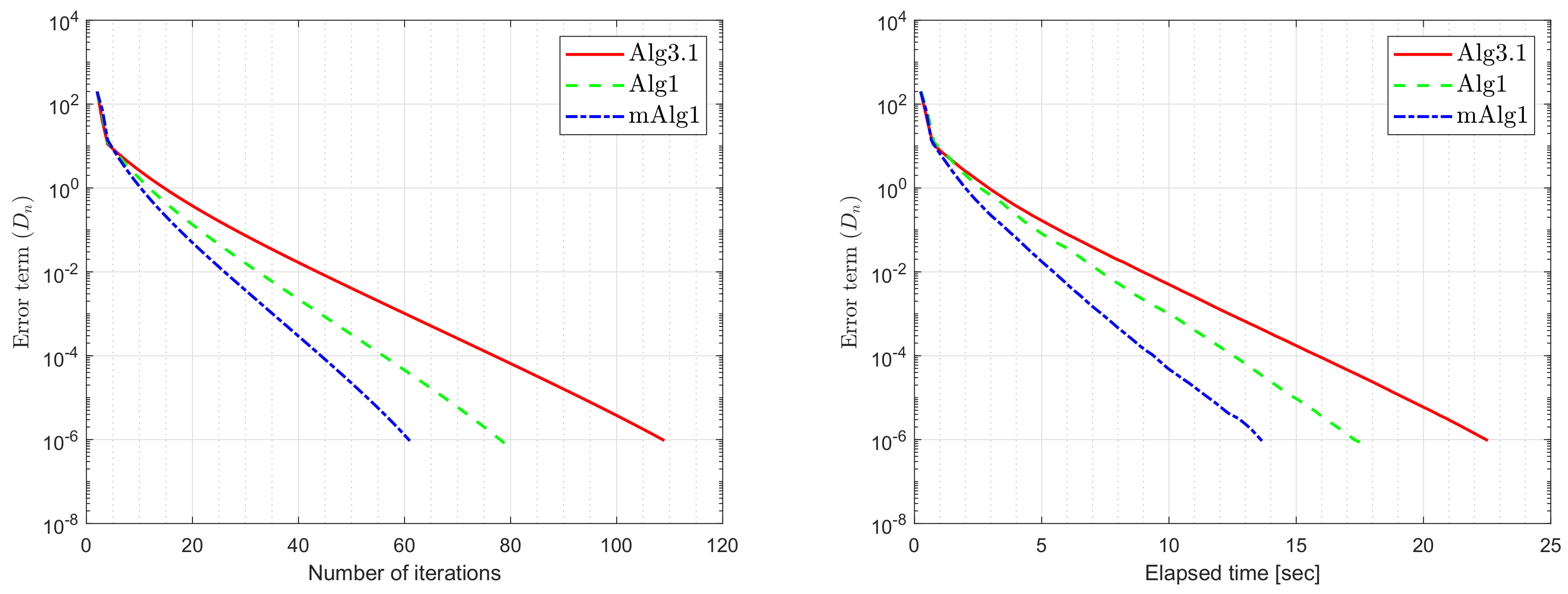
	Number of Iterations			Execution Time in Seconds
$\mathit{m}$	Alg3.1	Alg1	mAlg1	Alg3.1	Alg1	mAlg1
20	90	64	50	1.0089	0.6923	0.5541
50	98	70	52	1.6089	1.9092	0.8464
100	104	74	58	2.9231	2.1456	1.6970
200	109	79	61	22.5299	17.6267	13.6542
300	112	81	63	52.6776	39.0018	36.6305

Remark 2.

(i)

It is also significant that the value of ${\xi }_0$ is crucial and performs best when it is nearer to $1.$

(ii)

It is observed that the selection of the value ϑ is often significant and roughly the value $\vartheta \in (3,6)$ performs better than most other values.

7. Conclusions

In this paper, we consider the convergence result for pseudomonotone equilibrium problems that involve Lipschitz-type continuous bifunction but the Lipschitz-type constants are unknown. We modify the extragradient methods with an inertial term and new step size formula. Weak convergence theorem is proved for sequences generated by the algorithm. Several numerical experiments confirm the effectiveness of the proposed algorithms.

References

- Blum, E. From optimization and variational inequalities to equilibrium problems. Math. Stud. 1994, 63, 123–145. [Google Scholar]
- Fan, K. A Minimax Inequality and Applications, Inequalities III; Shisha, O., Ed.; Academic Press: New York, NY, USA, 1972. [Google Scholar]
- Facchinei, F.; Pang, J.S. Finite-Dimensional Variational Inequalities and Complementarity Problems; Springer Science & Business Media: Berlin, Germany, 2007. [Google Scholar]
- Konnov, I. Equilibrium Models and Variational Inequalities; Elsevier: Amsterdam, The Netherlands, 2007; Volume 210. [Google Scholar]
- Muu, L.D.; Oettli, W. Convergence of an adaptive penalty scheme for finding constrained equilibria. Nonlinear Anal. Theory Methods Appl. 1992, 18, 1159–1166. [Google Scholar] [CrossRef]
- Quoc, T.D.; Le Dung, M.N.V.H. Extragradient algorithms extended to equilibrium problems. Optimization 2008, 57, 749–776. [Google Scholar] [CrossRef]
- Quoc, T.D.; Anh, P.N.; Muu, L.D. Dual extragradient algorithms extended to equilibrium problems. J. Glob. Optim. 2011, 52, 139–159. [Google Scholar] [CrossRef]
- Lyashko, S.I.; Semenov, V.V. A New Two-Step Proximal Algorithm of Solving the Problem of Equilibrium Programming. In Optimization and Its Applications in Control and Data Sciences; Springer International Publishing: Berlin/Heidelberg, Germany, 2016; pp. 315–325. [Google Scholar] [CrossRef]
- Takahashi, S.; Takahashi, W. Viscosity approximation methods for equilibrium problems and fixed point problems in Hilbert spaces. J. Math. Anal. Appl. 2007, 331, 506–515. [Google Scholar] [CrossRef]
- ur Rehman, H.; Kumam, P.; Cho, Y.J.; Yordsorn, P. Weak convergence of explicit extragradient algorithms for solving equilibirum problems. J. Inequalities Appl. 2019, 2019. [Google Scholar] [CrossRef]
- Anh, P.N.; Hai, T.N.; Tuan, P.M. On ergodic algorithms for equilibrium problems. J. Glob. Optim. 2015, 64, 179–195. [Google Scholar] [CrossRef]
- Hieu, D.V.; Quy, P.K.; Vy, L.V. Explicit iterative algorithms for solving equilibrium problems. Calcolo 2019, 56. [Google Scholar] [CrossRef]
- Hieu, D.V. New extragradient method for a class of equilibrium problems in Hilbert spaces. Appl. Anal. 2017, 97, 811–824. [Google Scholar] [CrossRef]
- ur Rehman, H.; Kumam, P.; Je Cho, Y.; Suleiman, Y.I.; Kumam, W. Modified Popov’s explicit iterative algorithms for solving pseudomonotone equilibrium problems. Optim. Methods Softw. 2020, 1–32. [Google Scholar] [CrossRef]
- ur Rehman, H.; Kumam, P.; Abubakar, A.B.; Cho, Y.J. The extragradient algorithm with inertial effects extended to equilibrium problems. Comput. Appl. Math. 2020, 39. [Google Scholar] [CrossRef]
- Santos, P.; Scheimberg, S. An inexact subgradient algorithm for equilibrium problems. Comput. Appl. Math. 2011, 30, 91–107. [Google Scholar]
- Hieu, D.V. Halpern subgradient extragradient method extended to equilibrium problems. Revista de la Real Academia de Ciencias Exactas, Físicas y Naturales Serie A Matemáticas 2016, 111, 823–840. [Google Scholar] [CrossRef]
- ur Rehman, H.; Kumam, P.; Kumam, W.; Shutaywi, M.; Jirakitpuwapat, W. The Inertial Sub-Gradient Extra-Gradient Method for a Class of Pseudo-Monotone Equilibrium Problems. Symmetry 2020, 12, 463. [Google Scholar] [CrossRef]
- Anh, P.N.; An, L.T.H. The subgradient extragradient method extended to equilibrium problems. Optimization 2012, 64, 225–248. [Google Scholar] [CrossRef]
- Muu, L.D.; Quoc, T.D. Regularization Algorithms for Solving Monotone Ky Fan Inequalities with Application to a Nash-Cournot Equilibrium Model. J. Optim. Theory Appl. 2009, 142, 185–204. [Google Scholar] [CrossRef]
- ur Rehman, H.; Kumam, P.; Argyros, I.K.; Deebani, W.; Kumam, W. Inertial Extra-Gradient Method for Solving a Family of Strongly Pseudomonotone Equilibrium Problems in Real Hilbert Spaces with Application in Variational Inequality Problem. Symmetry 2020, 12, 503. [Google Scholar] [CrossRef]
- ur Rehman, H.; Kumam, P.; Argyros, I.K.; Alreshidi, N.A.; Kumam, W.; Jirakitpuwapat, W. A Self-Adaptive Extra-Gradient Methods for a Family of Pseudomonotone Equilibrium Programming with Application in Different Classes of Variational Inequality Problems. Symmetry 2020, 12, 523. [Google Scholar] [CrossRef]
- ur Rehman, H.; Kumam, P.; Argyros, I.K.; Shutaywi, M.; Shah, Z. Optimization Based Methods for Solving the Equilibrium Problems with Applications in Variational Inequality Problems and Solution of Nash Equilibrium Models. Mathematics 2020, 8, 822. [Google Scholar] [CrossRef]
- Yordsorn, P.; Kumam, P.; ur Rehman, H.; Ibrahim, A.H. A Weak Convergence Self-Adaptive Method for Solving Pseudomonotone Equilibrium Problems in a Real Hilbert Space. Mathematics 2020, 8, 1165. [Google Scholar] [CrossRef]
- Yordsorn, P.; Kumam, P.; Rehman, H.U. Modified two-step extragradient method for solving the pseudomonotone equilibrium programming in a real Hilbert space. Carpathian J. Math. 2020, 36, 313–330. [Google Scholar]
- La Sen, M.D.; Agarwal, R.P.; Ibeas, A.; Alonso-Quesada, S. On the Existence of Equilibrium Points, Boundedness, Oscillating Behavior and Positivity of a SVEIRS Epidemic Model under Constant and Impulsive Vaccination. Adv. Differ. Equ. 2011, 2011, 1–32. [Google Scholar] [CrossRef]
- La Sen, M.D.; Agarwal, R.P. Some fixed point-type results for a class of extended cyclic self-mappings with a more general contractive condition. Fixed Point Theory Appl. 2011, 2011. [Google Scholar] [CrossRef]
- Wairojjana, N.; ur Rehman, H.; Argyros, I.K.; Pakkaranang, N. An Accelerated Extragradient Method for Solving Pseudomonotone Equilibrium Problems with Applications. Axioms 2020, 9, 99. [Google Scholar] [CrossRef]
- La Sen, M.D. On Best Proximity Point Theorems and Fixed Point Theorems for -Cyclic Hybrid Self-Mappings in Banach Spaces. Abstr. Appl. Anal. 2013, 2013, 1–14. [Google Scholar] [CrossRef]
- ur Rehman, H.; Kumam, P.; Shutaywi, M.; Alreshidi, N.A.; Kumam, W. Inertial Optimization Based Two-Step Methods for Solving Equilibrium Problems with Applications in Variational Inequality Problems and Growth Control Equilibrium Models. Energies 2020, 13, 3292. [Google Scholar] [CrossRef]
- Rehman, H.U.; Kumam, P.; Dong, Q.L.; Peng, Y.; Deebani, W. A new Popov’s subgradient extragradient method for two classes of equilibrium programming in a real Hilbert space. Optimization 2020, 1–36. [Google Scholar] [CrossRef]
- Wang, L.; Yu, L.; Li, T. Parallel extragradient algorithms for a family of pseudomonotone equilibrium problems and fixed point problems of nonself-nonexpansive mappings in Hilbert space. J. Nonlinear Funct. Anal. 2020, 2020, 13. [Google Scholar]
- Shahzad, N.; Zegeye, H. Convergence theorems of common solutions for fixed point, variational inequality and equilibrium problems, J. Nonlinear Var. Anal. 2019, 3, 189–203. [Google Scholar]
- Farid, M. The subgradient extragradient method for solving mixed equilibrium problems and fixed point problems in Hilbert spaces. J. Appl. Numer. Optim. 2019, 1, 335–345. [Google Scholar]
- Flåm, S.D.; Antipin, A.S. Equilibrium programming using proximal-like algorithms. Math. Program. 1996, 78, 29–41. [Google Scholar] [CrossRef]
- Korpelevich, G. The extragradient method for finding saddle points and other problems. Matecon 1976, 12, 747–756. [Google Scholar]
- Yang, J.; Liu, H.; Liu, Z. Modified subgradient extragradient algorithms for solving monotone variational inequalities. Optimization 2018, 67, 2247–2258. [Google Scholar] [CrossRef]
- Vinh, N.T.; Muu, L.D. Inertial Extragradient Algorithms for Solving Equilibrium Problems. Acta Math. Vietnam. 2019, 44, 639–663. [Google Scholar] [CrossRef]
- Hieu, D.V.; Cho, Y.J.; bin Xiao, Y. Modified extragradient algorithms for solving equilibrium problems. Optimization 2018, 67, 2003–2029. [Google Scholar] [CrossRef]
- Bianchi, M.; Schaible, S. Generalized monotone bifunctions and equilibrium problems. J. Optim. Theory Appl. 1996, 90, 31–43. [Google Scholar] [CrossRef]
- Mastroeni, G. On Auxiliary Principle for Equilibrium Problems. In Nonconvex Optimization and Its Applications; Springer: New York, NY, USA, 2003; pp. 289–298. [Google Scholar] [CrossRef]
- Kreyszig, E. Introductory Functional Analysis with Applications, 1st ed.; Wiley Classics Library, Wiley: Hoboken, NJ, USA, 1989. [Google Scholar]
- Tiel, J.V. Convex Analysis: An Introductory Text, 1st ed.; Wiley: New York, NY, USA, 1984. [Google Scholar]
- Ioffe, A.D.; Tihomirov, V.M. (Eds.) Theory of Extremal Problems. In Studies in Mathematics and Its Applications 6; North-Holland, Elsevier: Amsterdam, The Netherlands; New York, NY, USA, 1979. [Google Scholar]
- Opial, Z. Weak convergence of the sequence of successive approximations for nonexpansive mappings. Bull. Amer. Math. Soc. 1967, 73, 591–598. [Google Scholar] [CrossRef]
- Tan, K.; Xu, H. Approximating Fixed Points of Nonexpansive Mappings by the Ishikawa Iteration Process. J. Math. Anal. Appl. 1993, 178, 301–308. [Google Scholar] [CrossRef]
- Bauschke, H.H.; Combettes, P.L. Convex Analysis and Monotone Operator Theory in Hilbert Spaces; Springer: New York, NY, USA, 2011; Volume 408. [Google Scholar]
- Browder, F.; Petryshyn, W. Construction of fixed points of nonlinear mappings in Hilbert space. J. Math. Anal. Appl. 1967, 20, 197–228. [Google Scholar] [CrossRef]