Inertial Subgradient Extragradient Methods for Solving Variational Inequality Problems and Fixed Point Problems

Abstract

We propose two new iterative algorithms for solving K-pseudomonotone variational inequality problems in the framework of real Hilbert spaces. These newly proposed methods are obtained by combining the viscosity approximation algorithm, the Picard Mann algorithm and the inertial subgradient extragradient method. We establish some strong convergence theorems for our newly developed methods under certain restriction. Our results extend and improve several recently announced results. Furthermore, we give several numerical experiments to show that our proposed algorithms performs better in comparison with several existing methods.

1. Introduction

In this paper, the set C denotes a nonempty closed convex subset of a real Hilbert space $H.$ The inner product of H is denoted by $⟨.,.⟩$ and the induced norm by $\parallel .\parallel .$ Suppose $A:H\to H$ is an operator. The variational inequality problem (VIP) for the operator A on $C\subset H$ is to find a point $x^{*}\in C$ such that

$$⟨A{x}^{*},x-x^{*}⟩\ge 0 \mathrm{for} \mathrm{each} x\in C.$$

(1)

In this study, we denote the solution set of (VIP) (1) by $\mathsf{\Gamma }.$ The theory of variational inequalities was introduced by Stampacchia [1]. It is known that the (VIP) problem arise in various models involving problems in many fields of study such as mathematics, physics, sciences, social sciences, management sciences, engineering and so on. The ideas and methods of the variational inequalities have been highly applied innovatively in diverse areas of sciences and engineering and have proved very effective in solving certain problems. The theory of (VIP) provides a natural, simple and unified setting for a comprehensive treatment of unrelated problems (see, e.g., [2]). Several authors have developed efficient numerical methods in solving the (VIP) problem. These methods includes the projection methods and its variants (see, e.g., [3,4,5,6,7,8,9,10,11,12,13]). The fundamental objective involves extending the well-known projected gradient algorithm, which is useful in solving the minimization problem $f\left(x\right)$ subject to $x\in C.$ This method is given as follows:

$$x_{n+1}=P_C(x_n-{\alpha }_n▽f\left(x_n\right)),\hspace{1em}n\ge 0,$$

(2)

where the real sequence $\left\{{\alpha }_n\right\}$ satisfy certain conditions and $P_C$ is the well-known metric projection onto $C\subset H.$ The interested reader may consult [14] for convergence analysis of this algorithm for the special case in which the mapping $f:H\to \mathbb{R}$ is convex and differentiable. Equation (2) has been extended to the (VIP) problem and it is known as the projected gradient method for optimization problems. This is done by replacing the gradient with the operator A thereby generating a sequence $\left\{x_n\right\}$ as follows:

$$x_{n+1}=P_C(x_n-{\alpha }_{n}A{x}_n),\hspace{1em}n\ge 0.$$

(3)

However, the major drawback of this method is the restrictive condition that the operator A is strongly monotone or inverse strongly monotone (see, e.g., [15]) to guarantee the convergence of this method. In 1976, Korpelevich [16] removed this strong condition by introducing the extragradient method for solving saddle point problems. The extragradient method was extended to solving variational inequality problems in both Hilbert and Euclidean spaces. The only required restriction for the extragradient algorithm to converge is that the operator A is monotone and L-Lipschitz continuous. The extragradient method is given as follows:

$$\left\{\begin{array}{c}{y}_n=P_C(x_n-\tau A{x}_n)\hfill \\ x_{n+1}=P_C(x_n-\tau A{y}_n),\hfill \end{array}\right.$$

(4)

where $\tau \in (0,\frac{1}{L})$ and the metric projection from H onto C is denoted by $P_C.$ If the solution set of the (VIP) denoted by $\mathsf{\Gamma }$ is nonempty, then the sequence $\left\{x_n\right\}$ generated by iterative algorithm (4) converges weakly to an element in $\mathsf{\Gamma }.$

Observe that by using the extragradient method, we need to calculate two projections onto the set $C\subset H$ in every iteration. It is known that the projection onto a closed convex set $C\subset H$ has a close relationship with the minimun distance problem. Let C be a closed and convex set, this method may require a prohibitive amount of computation time. In view of this drawback, in 2011 Censor et al. [5] introduced the subgradient extragradient method by modifying iterative algorithm in Equation (4) above. They replaced the two projections in the extragradient method in Equation (4) onto the set C by only one projection onto the set $C\subset H$ and one onto a half-space. It has been established that the projection onto a given half-space is easier to calculate. Next, we give the subgradient extragradient method of Censor et al. [5] as follows:

$$\left\{\begin{array}{c}{y}_n=P_C(x_n-\tau A{x}_n)\hfill \\ T_n=\{x\in H|⟨x_n-\tau A{x}_n-y_n,x-y_n⟩\le 0\}\hfill \\ x_{n+1}=P_{T_n}(x_n-\tau A{y}_n),\hfill \end{array}\right.$$

(5)

where $\tau \in (0,\frac{1}{L}).$ Several authors have studied the subgradient extragradient method and obtained some interesting and applicable results (see, e.g., [11]) and the references therein.

The theory of pseudomonotone operators is very crucial in studies in nonlinear analysis, variational inequalities and optimization problems (see, e.g., [17,18,19,20]). One important class of pseudomonotone operators was introduced in 1976 by Karamardian [21] and have been utilized in solving problems in variational inequalities, optimization and economics (see, e.g., [17,20]). In this paper, we shall call the class of pseudomonotone in the sense of Karamardian K-pseudomonotone. Yao [20] utilized K-pseudomonotone in solving some variational inequalities problems in Banach spaces. He established some new existence results which extend many known results in infinite-dimensional spaces under some weak assumptions. He also proved some uniqueness results for the complementarity problem with K-pseudomonotone operators in Banach spaces. It is our purpose in the present paper to introduce two new inertial subgradient extragradient iterative algorithms for solving K-pseudomonotone variational inequality problems in the framework of real Hilbert spaces.

The inertial type iterative algorithms are based on a discrete version of a second order dissipative dynamical system (see, [22,23]). These kind of algorithms can be seen as a process of accelerating the convergence properties of a given method (see, e.g., [24,25,26]). Alvarez and Attouch [24] in 2001 used the inertial method to derive a proximal algorithm for solving the problem of finding zero of a maximal monotone operator. Their method is given as follows: given $x_{n-1},x_n\in H$ and any two parameters ${\theta }_n\in [0,1),$${\lambda }_n>0,$ obtain $x_{n+1}\in H$ such that

$$0\in {\lambda }_{n}A\left(x_{n+1}\right)+x_{n+1}-x_n-{\theta }_n(x_n-x_{n-1}).$$

(6)

This algorithm can be written equivalently as follows:

$$x_{n+1}=J_{{\lambda }_n}^A(x_n+{\theta }_n(x_n-x_{n-1}),$$

(7)

where $J_{{\lambda }_n}^A$ is the resolvent of the operator A with the given parameter ${\lambda }_n$ and the inertial is induced by the term ${\theta }_n(x_n-x_{n-1}).$

Several researchers have developed some fast iterative algorithms by using inertial methods. These methods includes the inertial Douglas–Rachford splitting method (see, e.g., [27]), inertial forward–backward splitting methods (see, e.g., [28]), inertial ADMM (see, e.g., [29]), inertial proximal–extragradient method (see, e.g., [30]), inertial forward–backward–forward method (see, e.g., [31]), inertial contraction method (see, e.g., [32]), inertial Tseng method (see, e.g., [33]) and inertial Mann method (see, e.g., [11]).

Inspired by the results above, we propose two inertial subgradient extragradient methods for finding a solution of K-pseudomonotone and Lipschitz continuous (VIP). Our first proposed iterative algorithm is a hybrid of the inertial subgradient extragradient method [11], the viscosity method [34] and the Picard Mann method [35]. Our second method combines the inertial subgradient extragradient method [11] and the Picard Mann method [35].

This paper is organized as follows. In Section 2, we give some preliminary definitions of concepts and results that will be crucial in this study. In Section 3, we present our proposed iterative algorithms and prove some convergence results for them. In Section 4, we present some numerical experiments to support the convergence of our proposed iterative algorithms. In Section 5, we give the concluding remarks of the study.

2. Preliminaries

In this paper, the set C denotes a nonempty closed convex subset of a real Hilbert space $H.$ The inner product of H is denoted by $⟨.,.⟩$ and the induced norm by $\parallel .\parallel .$

We denote the weak convergence of the sequence $\left\{x_n\right\}$ to x by $x_n\rightharpoonup x$ as $n\to \infty ,$ we denote the strong convergence of $\left\{x_n\right\}$ to x by $x_n\to x$ as $n\to \infty .$

For each $x,y\in H$ and $\alpha \in \mathbb{R},$ we recall the following inequalities in Hilbert spaces:

$${\parallel \alpha x+(1-\alpha )y\parallel }^2={\alpha \parallel x\parallel }^2+{(1-\alpha )\parallel y\parallel }^2-\alpha (1-\alpha ){\parallel x-y\parallel }^2.$$

(8)

$${\parallel x+y\parallel }^2\le {\parallel x\parallel }^2+2⟨y,x+y⟩.$$

(9)

$${\parallel x+y\parallel }^2={\parallel x\parallel }^2+2⟨x,y⟩+{\parallel y\parallel }^2.$$

(10)

A mapping $A:H\to H$ is said to be nonexpansive if for each $x,y\in H,$ we have

$$\parallel Ax-Ay\parallel \le \parallel x-y\parallel .$$

For each $x\in H,$ we can find a unique nearest point in $C\subset H,$ denoted by $P_{C}x$ such that we have

$$\parallel x-P_{C}x\parallel \le \parallel x-y\parallel$$

(11)

for each $y\in C.$ Then $P_C$ is known as the metric projection of H onto $C\subset H.$ It has been proved that the mapping $P_C$ is nonexpansive.

Lemma 1

([36]). Suppose that C is a closed convex subset of a real Hilbert space H and for each $x\in H.$ Then the following holds:

(i) 

$\parallel P_{C}x-P_C{y\parallel }^2\le ⟨P_{C}x-P_{C}y,x-y⟩$ for all $y\in H.$

(ii) 

$\parallel P_C{x-y\parallel }^2\le {\parallel x-y\parallel }^2-{\parallel x-P_{C}x\parallel }^2$ for all $y\in H.$

(iii) 

Given $x\in H$ and $z\in C.$ Then we have

$$z=P_{C}x⟺⟨x-z,z-y⟩\ge 0$$

for all $y\in C.$

For more of the metric projection $P_C,$ the interested reader should see Section 3 of [36].

The fixed point problem involves finding the fixed point of an operator $A:H\to H.$ The set of fixed point of the operator A is denoted by $F\left(A\right)$ and we assume that it is nonempty, that is $F\left(A\right)\ne \varnothing .$ The fixed point problem $\left(FP\right)$ is then formulated as follows:

$$\mathrm{find}\hspace{1em}x\in H\hspace{1em}\mathrm{such} \mathrm{that} x=A\left(x\right).$$

(12)

In this paper, our problem of interest is to find a point $x\in H$ such that

$$x\in \mathsf{\Gamma }\cap F\left(A\right).$$

(13)

Definition 1.

Let $A:H\to H$ be a mapping. Then for all $x,y\in H$

(i) 

A is said to be L-Lipschitz continuous with $L>0$ if

$$\parallel Ax-Ay\parallel \le L\parallel x-y\parallel .$$

(14)

If $L\in [0,1)$ then A is called a contraction mapping.

(ii) 

A is said to be monotone if

$$⟨Ax-Ay,x-y⟩\ge 0.$$

(15)

(iii) 

The mapping $A:H\to H$ is said to be pseudomonotone in the sense of Karamardian [21] or K-pseudomonotone for short, if for all $x,y\in H$

$$⟨Ay,x-y⟩\ge 0\Rightarrow ⟨Ax,x-y⟩\ge 0.$$

(16)

The following lemmas will be needed in this paper.

Lemma 2.

([37]). Suppose $\left\{x_n\right\}$ is a real sequence of nonnegative numbers such that there is a subsequence $\left\{x_{n_j}\right\}$ of $\left\{x_n\right\}$ such that $x_{n_j}<x_{n_{j+1}}$ for any $j\in \mathbb{N}.$ Then there is a nondecreasing sequence $\left\{m_k\right\}$ of $\mathbb{N}$ such that ${lim}_{k\to \infty }{m}_k=\infty$ and the following properties are fulfilled: for each (sufficiently large) number $k\in \mathbb{N},$

$$x_{m_k}\le x_{m_{k+1}},\hspace{1em}{x}_k\le x_{m_{k+1}}.$$

In fact, $m_k$ is the largest number n in the set $\{1,2,\cdots ,k\}$ such that $x_n<x_{n+1}.$

Lemma 3.

([38]). Let $\left\{a_n\right\}$ be a sequence of nonnegative real numbers such that

$$a_{n+1}\le (1-{\alpha }_n)a_n+{\alpha }_n{b}_n$$

for all $n\ge 0,$ where $\left\{{\alpha }_n\right\}\subset (0,1)$ and $\left\{b_n\right\}$ is a sequence such that

(a) 

${\sum }_{n=0}^{\infty }{\alpha }_n=\infty ;$

(b) 

${lim\; sup}_{n\to \infty }{b}_n\le 0.$

Then ${lim}_{n\to \infty }{a}_n=0.$

3. Main Results

The following condition will be needed in this study.

Condition 3.1

The operator $A:H\to H$ is K-pseudomonotone and L-Lipschitz continuous on the real Hilbert space $H,$ with the solution set of the (VIP) (1.1) $\mathsf{\Gamma }\ne \varnothing$ and the contraction mapping $f:H\to H$ with the contraction parameter $k\in [0,1).$ The feasible set $C\subset H$ is non-empty, closed and convex.

3.1. The Viscosity Inertial Subgradient Extragradient Algorithm

We propose the following algorithm

Algorithm 3.1

Step 0: Given $\tau \in (0,\frac{1}{L}).$ $\left\{{\alpha }_n\right\}\subset [0,\alpha )$ for some $\alpha >0$ and $\left\{{\beta }_n\right\}\subset (0,1)$ satisfying the following conditions:

$$\underset{n\to \infty }{lim}{\beta }_n=0,\hspace{1em}\sum _{n=1}^{\infty }{\beta }_n=\infty .$$

(17)

Choose initial $x_0,x_1\in C$ and set $n:=1.$

Step 1: Compute

$$w_n=x_n+{\alpha }_n(x_n-x_{n-1}),$$

(18)

$$y_n=P_C(w_n-\tau A{w}_n).$$

(19)

If $y_n=w_n,$ then stop, $y_n$ is a solution to the (VIP) problem. Otherwise, go to Step 2.

Step 2: Construct the half-space

$$T_n:=\left\{z\in H:⟨w_n-\tau A{w}_n-y_n,z-y_n⟩\le 0\right\}$$

(20)

and compute

$$z_n=P_{T_n}(w_n-\tau A{y}_n).$$

(21)

Step 3: Calculate

$$h_n=(1-{\beta }_n)z_n+{\beta }_{n}f\left(z_n\right),$$

(22)

and compute

$$x_{n+1}=f\left(h_n\right).$$

(23)

Let $n:=n+1$ and return to Step 1.

Next, we prove the following results which will be useful in this study.

Lemma 4.

Let $\left\{x_n\right\}$ be a sequence generated by Algorithm 3.1. Then

$$\parallel x_{n+1}{-p\parallel }^2\le \parallel w_n{-p\parallel }^2-(1-\tau L)\parallel y_n-x_{n+1}{\parallel }^2-(1-\tau L){\parallel y_n-w_n\parallel }^2,$$

(24)

for all $p\in \mathsf{\Gamma }.$

Proof. 

Since $p\in \mathsf{\Gamma }\subset C\subset T_n,$ then by Equation (10) and Lemma 2 (i) we have the following

$$\begin{array}{ccc}\parallel x_{n+1}{-p\parallel }^2\hfill & =\hfill & \parallel P_{T_n}(w_n-\tau A{y}_n)-P_{T_n}{p\parallel }^2\hfill \\ & \le \hfill & ⟨x_{n+1}-p,w_n-\tau A{y}_n-p⟩\hfill \\ & =\hfill & \frac{1}{2}\parallel x_{n+1}{-p\parallel }^2+\frac{1}{2}\parallel w_n-\tau A{y}_n{-p\parallel }^2-\frac{1}{2}{\parallel x_{n+1}-w_n+\tau A{y}_n\parallel }^2\hfill \\ & =\hfill & \frac{1}{2}\parallel x_{n+1}{-p\parallel }^2+\frac{1}{2}\parallel w_n{-p\parallel }^2+\frac{1}{2}{\tau }^2\parallel A{y}_n{\parallel }^2-⟨w_n-p,\tau A{y}_n⟩-\frac{1}{2}{\parallel x_{n+1}-w_n\parallel }^2\hfill \\ & & -\frac{1}{2}{\tau }^2{\parallel A{y}_n\parallel }^2-⟨x_{n+1}-w_n,\tau A{y}_n⟩\hfill \\ & =\hfill & \frac{1}{2}\parallel x_{n+1}{-p\parallel }^2+\frac{1}{2}\parallel w_n{-p\parallel }^2-\frac{1}{2}{\parallel x_{n+1}-w_n\parallel }^2-⟨x_{n+1}-p,\tau A{y}_n⟩.\hfill \end{array}$$

(25)

Hence, from Equation (25) we obtain

$$\parallel x_{n+1}{-p\parallel }^2\le \parallel w_n{-p\parallel }^2-{\parallel x_{n+1}-w_n\parallel }^2-2⟨x_{n+1}-p,\tau A{y}_n⟩.$$

(26)

Using the condition that A is K-pseudomonotone, we have that $2\tau ⟨A{y}_n,y_n-p⟩\ge 0.$ We now add this to the right hand side of inequality (25) to obtain the following

$$\begin{array}{ccc}\parallel x_{n+1}{-p\parallel }^2\hfill & \le \hfill & \parallel w_n{-p\parallel }^2-{\parallel x_{n+1}-w_n\parallel }^2-2⟨x_{n+1}-p,\tau A{y}_n⟩+2\tau ⟨A{y}_n,y_n-p⟩\hfill \\ & =\hfill & \parallel w_n{-p\parallel }^2-{\parallel x_{n+1}-w_n\parallel }^2-2\tau ⟨x_{n+1}-p,A{y}_n⟩+2\tau ⟨y_n-p,A{y}_n⟩\hfill \\ & =\hfill & \parallel w_n{-p\parallel }^2-{\parallel x_{n+1}-w_n\parallel }^2-2\tau ⟨x_{n+1}-y_n,A{y}_n⟩-2\tau ⟨y_n-p,A{y}_n⟩+\hfill \\ & & 2\tau ⟨y_n-p,A{y}_n⟩\hfill \\ & =\hfill & \parallel w_n{-p\parallel }^2-{\parallel x_{n+1}-w_n\parallel }^2-2\tau ⟨x_{n+1}-y_n,A{y}_n-A{w}_n⟩-2\tau ⟨x_{n+1}-y_n,A{w}_n⟩\hfill \\ & =\hfill & \parallel w_n{-p\parallel }^2-{\parallel x_{n+1}-w_n\parallel }^2+2\tau ⟨y_n-x_{n+1},A{y}_n-A{w}_n⟩+2\tau ⟨y_n-x_{n+1},A{w}_n⟩.\hfill \end{array}$$

(27)

Next, we have the following estimates using the condition that A is L-Lipschitz continuous

$$\begin{array}{ccc}2\tau ⟨y_n-x_{n+1},A{y}_n-A{w}_n⟩\hfill & \le \hfill & 2\tau \parallel y_n-x_{n+1}\parallel \parallel A{y}_n-A{w}_n\parallel \hfill \\ & \le \hfill & 2\tau L\parallel y_n-x_{n+1}\parallel \parallel y_n-w_n\parallel \hfill \\ & \le \hfill & \tau L\parallel y_n-x_{n+1}{\parallel }^2+\tau L{\parallel y_n-w_n\parallel }^2.\hfill \end{array}$$

(28)

Since $y_n=P_{T_n}(w_n-\tau A{y}_n)$ and $x_{n+1}\in T_n,$ we obtain $⟨w_n-\tau A{w}_n-y_n,x_{n+1}-y_n⟩\le 0.$ This implies that

$$\begin{array}{ccc}2\tau ⟨y_n-x_{n+1},A{w}_n⟩\hfill & \le \hfill & 2⟨y_n-w_n,x_{n+1}-y_n⟩\hfill \\ & =\hfill & \parallel x_{n+1}-w_n{\parallel }^2-\parallel y_n-w_n{\parallel }^2-{\parallel x_{n+1}-y_n\parallel }^2.\hfill \end{array}$$

(29)

Using Equations (28) and (29) in Equation (27), we obtain:

$$\begin{array}{ccc}\parallel x_{n+1}{-p\parallel }^2\hfill & \le \hfill & \parallel w_n{-p\parallel }^2-\parallel x_{n+1}-w_n{\parallel }^2+\tau L\parallel y_n-x_{n+1}{\parallel }^2+\tau L\parallel y_n-w_n{\parallel }^2+{\parallel x_{n+1}-w_n\parallel }^2\hfill \\ & & -\parallel y_n-w_n{\parallel }^2-{\parallel x_{n+1}-y_n\parallel }^2\hfill \\ & =\hfill & \parallel w_n{-p\parallel }^2-(1-\tau L)\parallel y_n-x_{n+1}{\parallel }^2-(1-\tau L){\parallel y_n-w_n\parallel }^2.\hfill \end{array}$$

(30)

The proof of Lemma 4 is completed. □

Next, we prove the following results for Algorithm 3.1.

Theorem 1.

Assume that the sequence $\left\{{\alpha }_n\right\}$ is chosen such that

$$\underset{n\to \infty }{lim}\frac{{\alpha }_n}{{\beta }_n}\parallel x_n-x_{n-1}\parallel =0.$$

(31)

Suppose that $\left\{x_n\right\}$ is a sequence generated by our Algorithm 3.1, then $\left\{x_n\right\}$ converges strongly to an element $p\in \mathsf{\Gamma },$ where we have that $p=P_{\mathsf{\Gamma }}\circ f\left(p\right).$

Proof. 

Claim I

We need to prove that the sequence $\left\{x_n\right\}$ is bounded, for each $p=P_{\mathsf{\Gamma }}\circ f\left(p\right).$ By Lemma 4 we have

$$\parallel z_n{-p\parallel }^2\le \parallel w_n{-p\parallel }^2-(1-\tau L)\parallel y_n-x_{n+1}{\parallel }^2-(1-\tau L){\parallel y_n-w_n\parallel }^2.$$

(32)

This implies that

$$\parallel z_n-p\parallel \le \parallel w_n-p\parallel .$$

(33)

Using Equation (18), we have

$$\begin{array}{ccc}\parallel w_n-p\parallel \hfill & =\hfill & \parallel x_n+{\alpha }_n(x_n-x_{n-1})-p\parallel \hfill \\ & \le \hfill & \parallel x_n-p\parallel +{\alpha }_n\parallel x_n-x_{n-1}\parallel \hfill \\ & =\hfill & \parallel x_n-p\parallel +{\beta }_n.\frac{{\alpha }_n}{{\beta }_n}\parallel x_n-x_{n-1}\parallel .\hfill \end{array}$$

(34)

Using the condition that ${lim}_{n\to \infty }\frac{{\alpha }_n}{{\beta }_n}\parallel x_n-x_{n-1}\parallel =0;$ it follows that there exist a constant ${\ell }_1\ge 0$ such that

$$\frac{{\alpha }_n}{{\beta }_n}\parallel x_n-x_{n-1}\parallel \le {\ell }_1,\hspace{1em}\mathrm{for} \mathrm{each} n\ge 0.$$

(35)

Hence, using Equations (34) and (35) in Equation (33) we obtain

$$\parallel z_n-p\parallel \le \parallel w_n-p\parallel \le \parallel x_n-p\parallel +{\beta }_n{\ell }_1.$$

(36)

Using (23) and the condition that f is a contraction mapping, we have

$$\begin{array}{ccc}\parallel x_{n+1}-p\parallel \hfill & =\hfill & \parallel f\left(h_n\right)-p\parallel \hfill \\ & =\hfill & \parallel f\left(h_n\right)-f\left(p\right)+f\left(p\right)-p\parallel \hfill \\ & \le \hfill & \parallel f\left(h_n\right)-f\left(p\right)\parallel +\parallel f\left(p\right)-p\parallel \hfill \\ & \le \hfill & k\parallel h_n-p\parallel +\parallel f\left(p\right)-p\parallel .\hfill \end{array}$$

(37)

By Equation (22), we have

$$\begin{array}{ccc}\parallel h_n-p\parallel \hfill & =\hfill & \parallel (1-{\beta }_n)z_n+{\beta }_{n}f\left(z_n\right)-p\parallel \hfill \\ & \le \hfill & (1-{\beta }_n)\parallel z_n-p\parallel +{\beta }_n\parallel f\left(z_n\right)-p\parallel \hfill \\ & \le \hfill & (1-{\beta }_n)\parallel z_n-p\parallel +{\beta }_n\parallel f\left(z_n\right)-f\left(p\right)\parallel +{\beta }_n\parallel f\left(p\right)-p\parallel \hfill \\ & \le \hfill & (1-{\beta }_n)\parallel z_n-p\parallel +{\beta }_{n}k\parallel z_n-p\parallel +{\beta }_n\parallel f\left(p\right)-p\parallel \hfill \\ & =\hfill & (1-{\beta }_n(1-k))\parallel z_n-p\parallel +{\beta }_n\parallel f\left(p\right)-p\parallel .\hfill \end{array}$$

(38)

Using Equation (38) in Equation (37), we obtain:

$$\begin{array}{ccc}\parallel x_{n+1}-p\parallel \hfill & \le \hfill & k\left[(1-{\beta }_n(1-k))\parallel z_n-p\parallel +{\beta }_n\parallel f\left(p\right)-p\parallel \right]+\parallel f\left(p\right)-p\parallel \hfill \\ & =\hfill & k(1-{\beta }_n(1-k))\parallel z_n-p\parallel +k{\beta }_n\parallel f\left(p\right)-p\parallel +\parallel f\left(p\right)-p\parallel \hfill \\ & \le \hfill & k(1-{\beta }_n(1-k))\parallel z_n-p\parallel +k\parallel f\left(p\right)-p\parallel +\parallel f\left(p\right)-p\parallel \hfill \\ & =\hfill & k(1-{\beta }_n(1-k))\parallel z_n-p\parallel +(1+k)\parallel f\left(p\right)-p\parallel .\hfill \end{array}$$

(39)

Using Equation (36) in Equation (39), we have

$$\begin{array}{ccc}\parallel x_{n+1}-p\parallel \hfill & \le \hfill & k(1-{\beta }_n(1-k))\parallel x_n-p\parallel +k{\beta }_n{\ell }_1+(1+k)\parallel f\left(p\right)-p\parallel \hfill \\ & \le \hfill & k(1-{\beta }_n(1-k))\parallel x_n-p\parallel +k{\ell }_1+(1+k)\parallel f\left(p\right)-p\parallel \hfill \\ & \le \hfill & max\{\parallel x_n-p\parallel ,{\ell }_1+2\parallel f\left(p\right)-p\parallel \}\hfill \\ & ⋮\hfill & \\ & \le \hfill & max\{\parallel x_0-p\parallel ,{\ell }_1+2\parallel f\left(p\right)-p\parallel \}.\hfill \end{array}$$

(40)

This means that $\left\{x_n\right\}$ is bounded. Hence, it follows that $\left\{z_n\right\},$$\left\{f\left(z_n\right)\right\},$$\left\{h_n\right\},$$\left\{f\left(h_n\right)\right\}$ and $\left\{w_n\right\}$ are bounded.

Claim II

$$(1-\tau L)\parallel y_n-w_n{\parallel }^2+(1-\tau L)\parallel y_n-x_{n+1}{\parallel }^2\le \parallel x_n{-p\parallel }^2-{\parallel x_{n+1}-p\parallel }^2+{\beta }_n{\ell }_5,$$

(41)

for some ${\ell }_5>0.$ By Equation (23), we have

$$\begin{array}{ccc}\parallel x_{n+1}{-p\parallel }^2\hfill & =\hfill & \parallel f\left(h_n\right){-p\parallel }^2\hfill \\ & =\hfill & \parallel f\left(h_n\right)-f\left(p\right)+f\left(p\right){-p\parallel }^2\hfill \\ & \le \hfill & {\left(\parallel f\left(h_n\right)-f\left(p\right)\parallel +\parallel f\left(p\right)-p\parallel \right)}^2\hfill \\ & \le \hfill & {\left(k\parallel h_n-p\parallel +\parallel f\left(p\right)-p\parallel \right)}^2\hfill \\ & \le \hfill & \parallel h_n{-p\parallel }^2+2\parallel h_n{-p\parallel \parallel f\left(p\right)-p\parallel +\parallel f\left(p\right)-p\parallel }^2\hfill \\ & \le \hfill & \parallel h_n{-p\parallel }^2+{\ell }_2,\hfill \end{array}$$

(42)

for some ${\ell }_2>0.$ From Equation (22), we have

$$\begin{array}{ccc}\parallel h_n{-p\parallel }^2\hfill & =\hfill & \parallel (1-{\beta }_n)z_n+{\beta }_{n}f\left(z_n\right){-p\parallel }^2\hfill \\ & \le \hfill & (1-{\beta }_n)\parallel z_n{-p\parallel }^2+{\beta }_n{\parallel f\left(z_n\right)-p\parallel }^2\hfill \\ & \le \hfill & (1-{\beta }_n)\parallel z_n{-p\parallel }^2+{\beta }_n(\parallel f\left(z_n\right)-f\left(p\right)\parallel +\parallel f\left(p\right)-p{\parallel )}^2\hfill \\ & \le \hfill & (1-{\beta }_n)\parallel z_n{-p\parallel }^2+{\beta }_n(k\parallel z_n-p\parallel +\parallel f\left(p\right)-p{\parallel )}^2\hfill \\ & \le \hfill & (1-{\beta }_n)\parallel z_n{-p\parallel }^2+2{\beta }_n\parallel z_n-p\parallel \parallel f\left(p\right)-p\parallel +{\beta }_n\parallel z_n{-p\parallel }^2+{\beta }_n{\parallel f\left(p\right)-p\parallel }^2\hfill \\ & =\hfill & \parallel z_n{-p\parallel }^2+{\beta }_n(2\parallel z_n{-p\parallel \parallel f\left(p\right)-p\parallel +\parallel f\left(p\right)-p\parallel }^2)\hfill \\ & \le \hfill & \parallel z_n{-p\parallel }^2+{\beta }_n{\ell }_3,\hfill \end{array}$$

(43)

for some ${\ell }_3>0.$ Using Equation (32) in Equation (43), we obtain

$$\begin{array}{ccc}\parallel h_n{-p\parallel }^2\hfill & \le \hfill & \parallel w_n{-p\parallel }^2-(1-\tau L)\parallel y_n-x_{n+1}{\parallel }^2-(1-\tau L){\parallel y_n-w_n\parallel }^2+{\beta }_n{\ell }_3.\hfill \end{array}$$

(44)

From Equation (36), we have

$$\parallel w_n-p\parallel \le \parallel x_n-p\parallel +{\beta }_n{\ell }_1.$$

(45)

This implies that

$$\begin{array}{ccc}\parallel w_n{-p\parallel }^2\hfill & \le \hfill & (\parallel x_n-p{\parallel +{\beta }_n{\ell }_1)}^2\hfill \\ & =\hfill & \parallel x_n{-p\parallel }^2+{\beta }_n(2{\ell }_1\parallel x_n-p\parallel +{\beta }_n{\ell }_1^2)\hfill \\ & \le \hfill & \parallel x_n{-p\parallel }^2+{\beta }_n{\ell }_4,\hfill \end{array}$$

(46)

for some ${\ell }_4>0.$ Combining Equations (44) and (46), we have

$$\parallel h_n{-p\parallel }^2\le \parallel x_n{-p\parallel }^2+{\beta }_n{\ell }_4-(1-\tau L)\parallel y_n-x_{n+1}{\parallel }^2-(1-\tau L){\parallel y_n-w_n\parallel }^2+{\beta }_n{\ell }_3.$$

(47)

Using Equation (47) in Equation (42), we have

$$\parallel x_{n+1}{-p\parallel }^2\le \parallel x_n{-p\parallel }^2+{\beta }_n{\ell }_4-(1-\tau L)\parallel y_n-x_{n+1}\parallel -(1-\tau L)\parallel y_n-w_n{\parallel }^2+{\beta }_n{\ell }_3+{\beta }_n{\ell }_2.$$

(48)

This implies that

$$(1-\tau L)\parallel y_n-w_n{\parallel }^2+(1-\tau L)\parallel y_n-x_{n+1}{\parallel }^2\le \parallel x_n{-p\parallel }^2-{\parallel x_{n+1}-p\parallel }^2+{\beta }_n{\ell }_5,$$

(49)

where ${\ell }_5:={\ell }_2+{\ell }_3+{\ell }_4.$

Claim III

$$\begin{array}{ccc}\parallel x_{n+1}{-p\parallel }^2\hfill & \le \hfill & 2k(1-{\beta }_n(1-k)){\parallel x_n-p\parallel }^2+\hfill \\ & & 2{\beta }_n(1-k)\left[\frac{2k}{1-k}⟨f\left(p\right)-p,x_{n+1}-p⟩+\frac{3D}{1-k}.\frac{{\alpha }_n}{{\beta }_n}\parallel x_n-x_{n-1}\parallel +\frac{1}{{\beta }_n(1-k)}{\parallel f\left(p\right)-p\parallel }^2\right],\hfill \end{array}$$

(50)

for some $D>0.$ Using Equations (10) and (18), we have

$$\begin{array}{ccc}\parallel w_n{-p\parallel }^2\hfill & =\hfill & \parallel x_n+{\alpha }_n(x_n-x_{n-1}){-p\parallel }^2\hfill \\ & =\hfill & \parallel x_n{-p\parallel }^2+2{\alpha }_n⟨x_n-p,x_n-x_{n-1}⟩+{\alpha }_n^2{\parallel x_n-x_{n-1}\parallel }^2\hfill \\ & \le \hfill & \parallel x_n{-p\parallel }^2+2{\alpha }_n\parallel x_n-p\parallel \parallel x_n-x_{n-1}\parallel +{\alpha }_n^2\parallel x_n-x_{n-1}\parallel .\hfill \end{array}$$

(51)

By Equations (10) and (23), we have

$$\begin{array}{ccc}\parallel x_{n+1}{-p\parallel }^2\hfill & =\hfill & \parallel f\left(h_n\right){-p\parallel }^2\hfill \\ & =\hfill & \parallel f\left(h_n\right)-f\left(p\right)+f\left(p\right){-p\parallel }^2\hfill \\ & =\hfill & \parallel f\left(h_n\right)-f\left(p\right){\parallel }^2+{\parallel f\left(p\right)-p\parallel }^2+2⟨f\left(h_n\right)-f\left(p\right),f\left(p\right)-p⟩\hfill \\ & \le \hfill & k^2\parallel h_n{-p\parallel }^2{+\parallel f\left(p\right)-p\parallel }^2+2\parallel f\left(h_n\right)-f\left(p\right)\parallel \parallel f\left(p\right)-p\parallel \hfill \\ & \le \hfill & k^2\parallel h_n{-p\parallel }^2{+\parallel f\left(p\right)-p\parallel }^2+k^2\parallel h_n{-p\parallel }^2+{\parallel f\left(p\right)-p\parallel }^2\hfill \\ & \le \hfill & 2k\parallel h_n{-p\parallel }^2+2{\parallel f\left(p\right)-p\parallel }^2.\hfill \end{array}$$

(52)

Using Equations (9) and (22), we have

$$\begin{array}{ccc}\parallel h_n{-p\parallel }^2\hfill & =\hfill & \parallel {\beta }_{n}f\left(z_n\right)+(1-{\beta }_n)z_n{-p\parallel }^2\hfill \\ & =\hfill & \parallel {\beta }_n(f\left(z_n\right)-f\left(p\right))+(1-{\beta }_n)(z_n-p)+{\beta }_n(f\left(p\right)-p){\parallel }^2\hfill \\ & \le \hfill & \parallel {\beta }_n(f\left(z_n\right)-f\left(p\right))+(1-{\beta }_n)(z_n-p){\parallel }^2+2{\beta }_n⟨f\left(p\right)-p,x_{n+1}-p⟩\hfill \\ & \le \hfill & {\beta }_n\parallel f\left(z_n\right)-f\left(p\right){\parallel }^2+(1-{\beta }_n){\parallel z_n-p\parallel }^2+2{\beta }_n⟨f\left(p\right)-p,x_{n+1}-p⟩\hfill \\ & \le \hfill & {\beta }_n{k}^2\parallel z_n{-p\parallel }^2+(1-{\beta }_n){\parallel z_n-p\parallel }^2+2{\beta }_n⟨f\left(p\right)-p,x_{n+1}-p⟩\hfill \\ & \le \hfill & {\beta }_{n}k\parallel z_n{-p\parallel }^2+(1-{\beta }_n){\parallel z_n-p\parallel }^2+2{\beta }_n⟨f\left(p\right)-p,x_{n+1}-p⟩\hfill \\ & =\hfill & (1-{\beta }_n(1-k)){\parallel z_n-p\parallel }^2+2{\beta }_n⟨f\left(p\right)-p,x_{n+1}-p⟩\hfill \\ & \le \hfill & (1-{\beta }_n(1-k)){\parallel w_n-p\parallel }^2+2{\beta }_n⟨f\left(p\right)-p,x_{n+1}-p⟩.\hfill \end{array}$$

(53)

Using Equation (51) in Equation (53), we have

$$\begin{array}{c}\parallel h_n{-p\parallel }^2\le (1-{\beta }_n(1-k))\parallel x_n{-p\parallel }^2+2{\alpha }_n\parallel x_n-p\parallel \parallel x_n-x_{n-1}\parallel +{\alpha }_n^2{\parallel x_n-x_{n-1}\parallel }^2+2{\beta }_n⟨f\left(p\right)-p,x_{n+1}-p⟩.\end{array}$$

(54)

Using Equation (54) in Equation (52), we have:

$$\begin{array}{ccc}\parallel x_{n+1}{-p\parallel }^2\hfill & \le \hfill & 2k(1-{\beta }_n(1-k))\parallel x_n{-p\parallel }^2+4k{\alpha }_n\parallel x_n-p\parallel \parallel x_n-x_{n-1}\parallel +2k{\alpha }_n^2{\parallel x_n-x_{n-1}\parallel }^2\hfill \\ & & +4k{\beta }_n⟨f\left(p\right)-p,x_{n+1}-p⟩+2{\parallel f\left(p\right)-p\parallel }^2\hfill \\ & =\hfill & 2k(1-{\beta }_n(1-k))\parallel x_n{-p\parallel }^2+2k{\alpha }_n\parallel x_n-x_{n-1}\parallel \left(2\parallel x_n-p\parallel +{\alpha }_n\parallel x_n-x_{n-1}\parallel \right)+\hfill \\ & & 2(1-k)\left[\frac{2k{\beta }_n}{1-k}⟨f\left(p\right)-p,x_{n+1}-p⟩+\frac{1}{1-k}{\parallel f\left(p\right)-p\parallel }^2\right]\hfill \\ & \le \hfill & 2k(1-{\beta }_n(1-k))\parallel x_n{-p\parallel }^2+2k{\alpha }_n\parallel x_n-x_{n-1}\parallel \left(2\parallel x_n-p\parallel +\alpha \parallel x_n-x_{n-1}\parallel \right)+\hfill \\ & & 2(1-k)\left[\frac{2k{\beta }_n}{1-k}⟨f\left(p\right)-p,x_{n+1}-p⟩+\frac{1}{1-k}{\parallel f\left(p\right)-p\parallel }^2\right]\hfill \\ & \le \hfill & 2k(1-{\beta }_n(1-k))\parallel x_n{-p\parallel }^2+6D{\alpha }_n\parallel x_n-x_{n-1}\parallel +\hfill \\ & & 2(1-k)\left[\frac{2k{\beta }_n}{1-k}⟨f\left(p\right)-p,x_{n+1}-p⟩+\frac{1}{1-k}{\parallel f\left(p\right)-p\parallel }^2\right]\hfill \\ & \le \hfill & 2k(1-{\beta }_n(1-k)){\parallel x_n-p\parallel }^2+\hfill \\ & & 2{\beta }_n(1-k)\left[\frac{2k}{1-k}⟨f\left(p\right)-p,x_{n+1}-p⟩+\frac{3D}{1-k}.\frac{{\alpha }_n}{{\beta }_n}\parallel x_n-x_{n-1}\parallel +\frac{1}{{\beta }_n(1-k)}{\parallel f\left(p\right)-p\parallel }^2\right],\hfill \end{array}$$

(55)

where $D:={sup}_{n\in \mathbb{N}}\{\parallel x_n-p\parallel ,\alpha \parallel x_n-x_{n-1}\parallel \}>0.$

Claim IV

We need to prove that the sequence $\{\parallel x_n-p{\parallel }^2\}$ converges to zero by considering two possible cases.

Case I

There exists a number $N\in \mathbb{N}$ such that $\parallel x_{n+1}{-p\parallel }^2\le {\parallel x_n-p\parallel }^2$ for each $n\ge N.$ This implies that ${lim}_{n\to \infty }\parallel x_n-p\parallel$ exists and by Claim II, we have

$$\underset{n\to \infty }{lim}\parallel y_n-w_n\parallel =0,\hspace{1em}\underset{n\to \infty }{lim}\parallel y_n-x_{n+1}\parallel =0.$$

(56)

The fact that the sequence $\left\{x_n\right\}$ is bounded implies that there exists a subsequence $\left\{x_{n_k}\right\}$ of $\left\{x_n\right\}$ that converges weakly to some $z\in H$ such that

$$\underset{n\to \infty }{lim\; sup}⟨f\left(p\right)-p,x_n-p⟩=\underset{k\to \infty }{lim}⟨f\left(p\right)-p,x_{n_k}-p⟩=⟨f\left(p\right)-p,z-p⟩.$$

(57)

Using Equation (56) and Lemma 3, we get $z\in \mathsf{\Gamma }.$ From Equation (57) and the fact that $p=P_{\mathsf{\Gamma }}\circ f\left(p\right),$ we get

$$\underset{n\to \infty }{lim\; sup}⟨f\left(p\right)-p,x_n-p⟩=⟨f\left(p\right)-p,z-p⟩\le 0.$$

(58)

Next, we prove that

$$\underset{n\to \infty }{lim}\parallel x_{n+1}-x_n\parallel =0.$$

(59)

Clearly,

$$\parallel w_n-x_n\parallel ={\alpha }_n\parallel x_n-x_{n-1}\parallel =\frac{{\alpha }_n}{{\beta }_n}.{\beta }_n\parallel x_n-x_{n-1}\parallel ⟶0 \mathrm{as} n\to \infty .$$

(60)

Combining Equations (56) and (60) we have

$$\parallel x_{n+1}-x_n\parallel \le \parallel x_{n+1}-y_n\parallel +\parallel y_n-w_n\parallel +\parallel w_n-x_n\parallel ⟶0 \mathrm{as} n\to \infty .$$

(61)

Using Equations (58) and (59) we have

$$\underset{n\to \infty }{lim\; sup}⟨f\left(p\right)-p,x_{n+1}-p⟩\le \underset{n\to \infty }{lim\; sup}⟨f\left(p\right)-p,x_n-p⟩=⟨f\left(p\right)-p,z-p⟩\le 0.$$

(62)

Hence by Lemma 3 and Claim III we have ${lim}_{n\to \infty }\parallel x_n-p\parallel =0.$

Case II

We can find a subsequence $\{\parallel x_{n_j}-p{\parallel }^2\}$ of $\{\parallel x_n-p{\parallel }^2\}$ satisfying $\parallel x_{n_j}{-p\parallel }^2<{\parallel x_{n_j+1}-p\parallel }^2$ for each $j\in \mathbb{N}.$ Hence, by Lemma 2 it follows that we can find a nondecreasing real sequence $\left\{m_k\right\}$ of $\mathbb{N}$ satisfying ${lim}_{k\to \infty }{m}_k=\infty$ and we get the following inequalities for every $k\in \mathbb{N}$:

$$\parallel x_{m_k}{-p\parallel }^2\le \parallel x_{m_k+1}{-p\parallel }^2,\hspace{1em}\parallel x_k{-p\parallel }^2\le {\parallel x_{m_k}-p\parallel }^2.$$

(63)

By Claim II we get

$$(1-\tau L)\parallel y_{m_k}-w_{m_k}{\parallel }^2+(1-\tau L)\parallel y_{m_k}-x_{m_k+1}{\parallel }^2\le \parallel x_{m_k}{-p\parallel }^2-{\parallel x_{m_k+1}-p\parallel }^2+{\beta }_{m_k}{\ell }_5\le {\beta }_{m_k}{\ell }_5.$$

(64)

Hence, we have

$$\underset{k\to \infty }{lim}\parallel y_{m_k}-w_{m_k}\parallel =0,\hspace{1em}\underset{k\to \infty }{lim}\parallel y_{m_k}-x_{m_k+1}\parallel =0.$$

(65)

By similar arguments as in the proof of Case I, we have

$$\parallel x_{m_k+1}-x_{m_k}\parallel ⟶0\hspace{1em}\mathrm{as} k\to \infty ,$$

(66)

and

$$\underset{k\to \infty }{lim\; sup}⟨f\left(p\right)-p,x_{m_k+1}-p⟩\le 0.$$

(67)

By Claim III we obtain

$$\begin{array}{ccc}\parallel x_{m_k+1}{-p\parallel }^2\hfill & \le \hfill & 2k(1-{\beta }_{m_k}(1-k)){\parallel x_{m_k}-p\parallel }^2+\hfill \\ & & 2{\beta }_{m_k}(1-k)[\frac{2k}{1-k}⟨f\left(p\right)-p,x_{m_k+1}-p⟩+\frac{3D}{1-k}.\frac{{\alpha }_{m_k}}{{\beta }_{m_k}}\parallel x_{m_k}-x_{m_k-1}\parallel +\hfill \\ & & \frac{1}{{\beta }_{m_k}(1-k)}{\parallel f\left(p\right)-p\parallel }^2].\hfill \end{array}$$

(68)

By Equations (63) and (68) we have:

$$\begin{array}{ccc}\parallel x_{m_k+1}{-p\parallel }^2\hfill & \le \hfill & 2k(1-{\beta }_{m_k}(1-k)){\parallel x_{m_k}-p\parallel }^2+\hfill \\ & & 2{\beta }_{m_k}(1-k)[\frac{2k}{1 - k}⟨f\left(p\right)-p,x_{m_k+1}-p⟩+\frac{3D}{1 - k}.\frac{{\alpha }_{m_k}}{{\beta }_{m_k}}\parallel x_{m_k}-x_{m_k-1}\parallel +\hfill \\ & & \frac{1}{{\beta }_{m_k}(1 - k)}{\parallel f\left(p\right)-p\parallel }^2].\hfill \end{array}$$

(69)

Hence, we have

$$\begin{array}{ccc}\parallel x_{m_k+1}{-p\parallel }^2\hfill & \le \hfill & \frac{2k}{1 - k}⟨f\left(p\right)-p,x_{m_k+1}-p⟩+\frac{3D}{1 - k}.\frac{{\alpha }_{m_k}}{{\beta }_{m_k}}\parallel x_{m_k}-x_{m_k-1}\parallel +\frac{1}{{\beta }_{m_k}(1 - k)}{\parallel f\left(p\right)-p\parallel }^2.\hfill \end{array}$$

(70)

Therefore we obtain:

$$\underset{k\to \infty }{lim\; sup}\parallel x_{m_k+1}-p\parallel \le 0.$$

(71)

Combining Equations (63) and (71) we obtain ${lim\; sup}_{k\to \infty }\parallel x_k-p\parallel \le 0,$ this means that $x_k⟶p.$ The proof of Theorem 1 is completed. □

Remark 1.

Suantai et al. [39] observed that condition (31) can be easily implemented in numerical results since the value of $\parallel x_n-x_{n-1}\parallel$ is given before choosing ${\alpha }_n.$ We can choose ${\alpha }_n$ as follows:

$${\alpha }_n=\left\{\begin{array}{cc}min\left\{\alpha ,\frac{{\epsilon }_n}{\parallel x_n-x_{n-1}\parallel }\right\},\hfill & \mathit{if} x_n\ne x_{n-1},\hfill \\ \alpha \hfill & \mathit{otherwise},\hfill \end{array}\right.$$

where $\alpha \ge 0$ and $\left\{{\epsilon }_n\right\}$ is a positive sequence such that ${\epsilon }_n=o\left({\beta }_n\right).$

3.2. Picard–Mann Hybrid Type Inertial Subgradient Extragradient Algorithm

We propose the following algorithm

Algorithm 3.2

Step 0: Given $\tau \in (0,\frac{1}{L}).$ $\left\{{\alpha }_n\right\}\subset [0,\alpha )$ for some $\alpha >0,$ $\left\{{\lambda }_n\right\}\subset (a,b)\subset (0,1-{\beta }_n)$ and $\left\{{\beta }_n\right\}\subset (0,1)$ satisfying the following conditions:

$$\underset{n\to \infty }{lim}{\beta }_n=0,\hspace{1em}\sum _{n=1}^{\infty }{\beta }_n=\infty .$$

(72)

Choose initial $x_0,x_1\in C$ and set $n:=1.$

Step 1: Compute

$$w_n=x_n+{\alpha }_n(x_n-x_{n-1}),$$

(73)

$$y_n=P_C(w_n-\tau A{w}_n).$$

(74)

If $y_n=w_n,$ then stop, $y_n$ is a solution of the (VIP) problem. Otherwise, go to Step 2.

Step 2: Construct the half-space

$$T_n:=\left\{z\in H:⟨w_n-\tau A{w}_n-y_n,z-y_n⟩\le 0\right\}$$

(75)

and compute

$$z_n=P_{T_n}(w_n-\tau A{y}_n).$$

(76)

Step 3: Calculate

$$h_n=(1-{\lambda }_n-{\beta }_n)x_n+{\lambda }_n{z}_n,$$

(77)

and compute

$$x_{n+1}=f\left(h_n\right).$$

(78)

Let $n:=n+1$ and return to Step 1.

Next, we prove the following important result for Algorithm 3.2.

Theorem 2.

Suppose that $\left\{{\alpha }_n\right\}$ is a real sequence such that the following condition holds:

$$\underset{n\to \infty }{lim}\frac{{\alpha }_n}{{\beta }_n}\parallel x_n-x_{n-1}\parallel =0.$$

(79)

Then the sequence $\left\{x_n\right\}$ generated by Algorithm 3.2 converges strongly to an element $p\in \mathsf{\Gamma },$ where $\parallel p\parallel =min\{\parallel z\parallel :z\in \mathsf{\Gamma }\}.$

Proof. 

We now examine the following claims:

Claim I

We claim that the sequence $\left\{x_n\right\}$ is bounded. Using similar arguments as in the proof of Theorem 1, we get

$$\parallel z_n{-p\parallel }^2\le \parallel w_n{-p\parallel }^2-(1-\tau L)\parallel y_n-x_{n+1}{\parallel }^2-(1-\tau L){\parallel y_n-w_n\parallel }^2.$$

(80)

This implies that

$$\parallel z_n-p\parallel \le \parallel w_n-p\parallel .$$

(81)

Moreover, we have

$$\parallel z_n-p\parallel \le \parallel w_n-p\parallel \le \parallel x_n-p\parallel +{\beta }_n{\ell }_1,$$

(82)

for some ${\ell }_1>0.$

$$\parallel x_{n+1}-p\parallel \le k\parallel h_n-p\parallel +\parallel f\left(p\right)-p\parallel .$$

(83)

Using Equation (77) we have

$$\begin{array}{ccc}\parallel h_n-p\parallel \hfill & =\hfill & \parallel (1-{\lambda }_n-{\beta }_n)x_n+{\lambda }_n{z}_n-p\parallel \hfill \\ & =\hfill & \parallel (1-{\lambda }_n-{\beta }_n)(x_n-p)+{\lambda }_n(z_n-p)-{\beta }_{n}p\parallel \hfill \\ & \le \hfill & \parallel (1-{\lambda }_n-{\beta }_n)(x_n-p)+{\lambda }_n(z_n-p)\parallel +{\beta }_n\parallel p\parallel .\hfill \end{array}$$

(84)

Using Equations (10) and (82), we have the following estimate:

$$\begin{array}{ccc}\parallel (1-{\lambda }_n-{\beta }_n)(x_n-p)+{\lambda }_n(z_n-p){\parallel }^2\hfill & =\hfill & {(1-{\lambda }_n-{\beta }_n)}^2{\parallel x_n-p\parallel }^2+\hfill \\ & & 2(1-{\lambda }_n-{\beta }_n){\lambda }_n⟨x_n-p,z_n-p⟩+{\lambda }_n^2{\parallel z_n-p\parallel }^2\hfill \\ & \le \hfill & {(1-{\lambda }_n-{\beta }_n)}^2{\parallel x_n-p\parallel }^2+\hfill \\ & & 2(1-{\lambda }_n-{\beta }_n){\lambda }_n\parallel x_n-p\parallel \parallel z_n-p\parallel +{\lambda }_n^2{\parallel z_n-p\parallel }^2\hfill \\ & \le \hfill & {(1-{\lambda }_n-{\beta }_n)}^2\parallel x_n{-p\parallel }^2+(1-{\lambda }_n-{\beta }_n){\lambda }_n{\parallel x_n-p\parallel }^2+\hfill \\ & & (1-{\lambda }_n-{\beta }_n){\lambda }_n\parallel z_n{-p\parallel }^2+{\lambda }_n^2{\parallel z_n-p\parallel }^2\hfill \\ & \le \hfill & (1-{\lambda }_n-{\beta }_n)(1-{\beta }_n)\parallel x_n{-p\parallel }^2+(1-{\beta }_n){\lambda }_n{\parallel z_n-p\parallel }^2\hfill \end{array}$$

(85)

This implies that

$$\begin{array}{ccc}\parallel (1-{\lambda }_n-{\beta }_n)(x_n-p)+{\lambda }_n(z_n-p){\parallel }^2\hfill & \le \hfill & (1-{\lambda }_n-{\beta }_n)(1-{\beta }_n){\parallel x_n-p\parallel }^2+\hfill \\ & & (1-{\beta }_n){\lambda }_n(\parallel x_n-p{\parallel +{\beta }_n{\ell }_1)}^2\hfill \\ & \le \hfill & (1-{\lambda }_n-{\beta }_n)(1-{\beta }_n)\parallel x_n{-p\parallel }^2+(1-{\beta }_n){\lambda }_n{\parallel x_n-p\parallel }^2\hfill \\ & & +2(1-{\beta }_n){\lambda }_n{\beta }_n\parallel x_n-p\parallel {\ell }_1+{\beta }_n^2{\ell }_1^2\hfill \\ & \le \hfill & {(1-{\beta }_n)}^2\parallel x_n{-p\parallel }^2+2(1-{\beta }_n){\beta }_n\parallel x_n-p\parallel {\ell }_1+{\beta }_n^2{\ell }_1^2\hfill \\ & =\hfill & {\left\{(1-{\beta }_n)\parallel x_n-p\parallel +{\beta }_n{\ell }_1\right\}}^2.\hfill \end{array}$$

(86)

This implies that

$$\parallel (1-{\lambda }_n-{\beta }_n)(x_n-p)+{\lambda }_n(z_n-p)\parallel \le (1-{\beta }_n)\parallel x_n-p\parallel +{\beta }_n{\ell }_1.$$

(87)

Using Equation (87) in Equation (84), we get

$$\begin{array}{ccc}\parallel h_n-p\parallel \hfill & \le \hfill & (1-{\beta }_n)\parallel x_n-p\parallel +{\beta }_n{\ell }_1+{\beta }_n\parallel p\parallel \hfill \\ & =\hfill & (1-{\beta }_n)\parallel x_n-p\parallel +{\beta }_n({\ell }_1+\parallel p\parallel ).\hfill \end{array}$$

(88)

Using Equation (88) in Equation (83), we have

$$\begin{array}{ccc}\parallel x_{n+1}-p\parallel \hfill & \le \hfill & (1-{\beta }_n)\parallel x_n-p\parallel +{\beta }_n({\ell }_1+\parallel p\parallel )+\parallel f\left(p\right)-p\parallel \hfill \\ & \le \hfill & max\left\{\parallel x_n-p\parallel ,{\ell }_1+\parallel p\parallel +\parallel f\left(p\right)-p\parallel \right\}\hfill \\ & ⋮\hfill & \\ & \le \hfill & max\left\{\parallel x_0-p\parallel ,{\ell }_1+\parallel p\parallel +\parallel f\left(p\right)-p\parallel \right\}.\hfill \end{array}$$

(89)

Therefore, the sequence $\left\{x_n\right\}$ is bounded. It follows that $\left\{z_n\right\},$ $\left\{w_n\right\}$ and $\left\{h_n\right\}$ are all bounded.

Claim II

We want to show that

$$\begin{array}{c}(1-{\beta }_n){\lambda }_n(1-\tau L)\parallel y_n-x_{n+1}{\parallel }^2+(1-{\beta }_n){\lambda }_n(1-\tau L)\parallel y_n-w_n{\parallel }^2\le \parallel x_n{-p\parallel }^2-{\parallel x_{n+1}-p\parallel }^2+{\beta }_n{\ell }_6,\end{array}$$

(90)

for some ${\ell }_6>0.$ From Equation (42), we have

$$\parallel x_{n+1}{-p\parallel }^2\le {\parallel h_n-p\parallel }^2+{\ell }_2,$$

(91)

for some ${\ell }_2>0.$ Using (10) and (77) we get

$$\begin{array}{ccc}\parallel h_n{-p\parallel }^2\hfill & =\hfill & \parallel (1-{\lambda }_n-{\beta }_n)x_n+{\lambda }_n{z}_n{-p\parallel }^2\hfill \\ & =\hfill & \parallel (1-{\lambda }_n-{\beta }_n)(x_n-p)+{\lambda }_n(z_n-p)-{\beta }_n{p\parallel }^2\hfill \\ & =\hfill & \parallel (1-{\lambda }_n-{\beta }_n)(x_n-p)+{\lambda }_n(z_n-p){\parallel }^2-\hfill \\ & & 2{\beta }_n⟨(1-{\lambda }_n-{\beta }_n)(x_n-p)+{\lambda }_n(z_n-p),p⟩+{\beta }_n^2{\parallel p\parallel }^2\hfill \\ & \le \hfill & \parallel (1-{\lambda }_n-{\beta }_n)(x_n-p)+{\lambda }_n(z_n-p){\parallel }^2+{\beta }_n{\ell }_3,\hfill \end{array}$$

(92)

for some ${\ell }_3>0.$ Using Equation (85) in Equation (92), we get

$$\parallel h_n{-p\parallel }^2\le (1-{\lambda }_n-{\beta }_n)(1-{\beta }_n)\parallel x_n{-p\parallel }^2+(1-{\beta }_n){\lambda }_n{\parallel z_n-p\parallel }^2+{\beta }_n{\ell }_3.$$

(93)

Using Equation (80) in Equation (93), we get

$$\begin{array}{ccc}\parallel h_n{-p\parallel }^2\hfill & \le \hfill & (1-{\lambda }_n-{\beta }_n)(1-{\beta }_n)\parallel x_n{-p\parallel }^2+(1-{\beta }_n){\lambda }_n[\parallel w_n{-p\parallel }^2-\hfill \\ & & (1-\tau L)\parallel y_n-x_{n+1}{\parallel }^2-(1-\tau L)\parallel y_n-w_n{\parallel }^2]+{\beta }_n{\ell }_3\hfill \\ & =\hfill & (1-{\lambda }_n-{\beta }_n)(1-{\beta }_n)\parallel x_n{-p\parallel }^2+(1-{\beta }_n){\lambda }_n{\parallel w_n-p\parallel }^2-\hfill \\ & & (1-{\beta }_n){\lambda }_n(1-\tau L)\parallel y_n-x_{n+1}{\parallel }^2-(1-{\beta }_n){\lambda }_n(1-\tau L){\parallel y_n-w_n\parallel }^2+{\beta }_n{\ell }_3.\hfill \end{array}$$

(94)

From Equation (36), we get

$$\parallel z_n-p\parallel \le \parallel w_n-p\parallel \le \parallel x_n-p\parallel +{\beta }_n{\ell }_1.$$

(95)

This implies that

$$\parallel w_n{-p\parallel }^2\le {\parallel x_n-p\parallel }^2+{\beta }_n{\ell }_4,$$

(96)

for some ${\ell }_4>0.$ Using Equation (96) in Equation (94), we get

$$\begin{array}{ccc}\parallel h_n{-p\parallel }^2\hfill & \le \hfill & (1-{\lambda }_n-{\beta }_n)(1-{\beta }_n)\parallel x_n{-p\parallel }^2+(1-{\beta }_n){\lambda }_n[\parallel x_n-p{\parallel }^2+{\beta }_n{\ell }_4]-\hfill \\ & & (1-{\beta }_n){\lambda }_n(1-\tau L)\parallel y_n-x_{n+1}{\parallel }^2-(1-{\beta }_n){\lambda }_n(1-\tau L){\parallel y_n-w_n\parallel }^2+{\beta }_n{\ell }_3\hfill \\ & =\hfill & {(1-{\beta }_n)}^2\parallel x_n{-p\parallel }^2+{\beta }_n(1-{\beta }_n){\lambda }_n{\ell }_4-(1-{\beta }_n){\lambda }_n(1-\tau L){\parallel y_n-x_{n+1}\parallel }^2-\hfill \\ & & (1-{\beta }_n){\lambda }_n(1-\tau L){\parallel y_n-w_n\parallel }^2+{\beta }_n{\ell }_3\hfill \\ & \le \hfill & \parallel x_n{-p\parallel }^2-(1-{\beta }_n){\lambda }_n(1-\tau L){\parallel y_n-x_{n+1}\parallel }^2-\hfill \\ & & (1-{\beta }_n){\lambda }_n(1-\tau L){\parallel y_n-w_n\parallel }^2+{\beta }_n{\ell }_5,\hfill \end{array}$$

(97)

for some ${\ell }_5>0.$ Using Equation (97) in Equation (91), we have

$$\begin{array}{ccc}\parallel x_{n+1}{-p\parallel }^2\hfill & \le \hfill & \parallel x_n{-p\parallel }^2-(1-{\beta }_n){\lambda }_n(1-\tau L)\parallel y_n-x_{n+1}{\parallel }^2-(1-{\beta }_n){\lambda }_n(1-\tau L){\parallel y_n-w_n\parallel }^2\hfill \\ & & +{\beta }_n{\ell }_5+{\ell }_2\hfill \\ & \le \hfill & \parallel x_n{-p\parallel }^2-(1-{\beta }_n){\lambda }_n(1-\tau L)\parallel y_n-x_{n+1}{\parallel }^2-(1-{\beta }_n){\lambda }_n(1-\tau L){\parallel y_n-w_n\parallel }^2\hfill \\ & & +{\beta }_n{\ell }_6,\hfill \end{array}$$

(98)

for some ${\ell }_6>0.$ This implies that

$$\begin{array}{c}(1-{\beta }_n){\lambda }_n(1-\tau L)\parallel y_n-x_{n+1}{\parallel }^2+(1-{\beta }_n){\lambda }_n(1-\tau L)\parallel y_n-w_n{\parallel }^2\le \parallel x_n{-p\parallel }^2-{\parallel x_{n+1}-p\parallel }^2+{\beta }_n{\ell }_6.\hfill \end{array}$$

(99)

Claim III

We want to show that

$$\begin{array}{ccc}\parallel x_{n+1}{-p\parallel }^2\hfill & \le \hfill & 2k\parallel x_n{-p\parallel }^2+2k{\beta }_n[2(1-{\beta }_n)\parallel x_n-p\parallel {\ell }_9+\hfill \\ & & {\lambda }_n.\frac{{\alpha }_n}{{\beta }_n}\parallel x_n-x_{n-1}\parallel {\ell }_9+\frac{1}{k{\beta }_n}{\parallel f\left(p\right)-p\parallel }^2-2⟨(1-{\lambda }_n-{\beta }_n)(x_n-p),p⟩+3{\ell }_9],\hfill \end{array}$$

(100)

for some ${\ell }_9>0.$

Using Equations (10) and (78), we have

$$\begin{array}{ccc}\parallel x_{n+1}{-p\parallel }^2\hfill & =\hfill & \parallel f\left(h_n\right)-f\left(p\right)+f\left(p\right){-p\parallel }^2\hfill \\ & =\hfill & \parallel f\left(h_n\right)-f\left(p\right){\parallel }^2+{\parallel f\left(p\right)-p\parallel }^2+2⟨f\left(h_n\right)-f\left(p\right),f\left(p\right)-p⟩\hfill \\ & \le \hfill & k^2\parallel h_n{-p\parallel }^2+{\parallel f\left(p\right)-p\parallel }^2+2⟨f\left(h_n\right)-f\left(p\right),f\left(p\right)-p⟩\hfill \\ & \le \hfill & k\parallel h_n{-p\parallel }^2+{\parallel f\left(p\right)-p\parallel }^2+2⟨f\left(h_n\right)-f\left(p\right),f\left(p\right)-p⟩\hfill \\ & \le \hfill & k\parallel h_n{-p\parallel }^2{+\parallel f\left(p\right)-p\parallel }^2+2\parallel f\left(h_n\right)-f\left(p\right)\parallel \parallel f\left(p\right)-p\parallel \hfill \\ & \le \hfill & k\parallel h_n{-p\parallel }^2{+\parallel f\left(p\right)-p\parallel }^2+\parallel f\left(h_n\right)-f\left(p\right){\parallel }^2+{\parallel f\left(p\right)-p\parallel }^2\hfill \\ & \le \hfill & 2k\parallel h_n{-p\parallel }^2+2{\parallel f\left(p\right)-p\parallel }^2.\hfill \end{array}$$

(101)

Next, we have the following estimate, using Equations (10) and (77)

$$\begin{array}{ccc}\parallel h_n{-p\parallel }^2\hfill & =\hfill & \parallel (1-{\lambda }_n-{\beta }_n)x_n+{\lambda }_n{z}_n{-p\parallel }^2\hfill \\ & =\hfill & \parallel (1-{\lambda }_n-{\beta }_n)(x_n-p)+{\lambda }_n(z_n-p)-{\beta }_n{p\parallel }^2\hfill \\ & =\hfill & \parallel (1-{\lambda }_n-{\beta }_n)(x_n-p)+{\lambda }_n(z_n-p){\parallel }^2-\hfill \\ & & 2{\beta }_n⟨(1-{\lambda }_n-{\beta }_n)(x_n-p)+{\lambda }_n(z_n-p),p⟩+{\beta }_n^2{\parallel p\parallel }^2.\hfill \end{array}$$

(102)

Using Equation (86) in Equation (102), we have

$$\begin{array}{ccc}\parallel h_n{-p\parallel }^2\hfill & \le \hfill & \{(1-{\beta }_n)\parallel x_n-p\parallel +{\beta }_n{\ell }_1{\}}^2-2{\beta }_n⟨(1-{\lambda }_n-{\beta }_n)(x_n-p)+{\lambda }_n(z_n-p),p⟩+{\beta }_n^2{\parallel p\parallel }^2\hfill \\ & \le \hfill & (1-{\beta }_n)\parallel x_n{-p\parallel }^2+2(1-{\beta }_n){\beta }_n\parallel x_n-p\parallel {\ell }_7+{\beta }_n{\ell }_7^2-\hfill \\ & & 2{\beta }_n⟨(1-{\lambda }_n-{\beta }_n)(x_n-p)+{\lambda }_n(z_n-p),p⟩+{\beta }_n^2{\parallel p\parallel }^2\hfill \\ & =\hfill & (1-{\beta }_n)\parallel x_n{-p\parallel }^2+2(1-{\beta }_n){\beta }_n\parallel x_n-p\parallel {\ell }_7+{\beta }_n{\ell }_7^2-2{\beta }_n⟨(1-{\lambda }_n-{\beta }_n)(x_n-p),p⟩\hfill \\ & & -2{\lambda }_n{\beta }_n⟨z_n-p,p⟩+{\beta }_n^2{\parallel p\parallel }^2\hfill \\ & =\hfill & (1-{\beta }_n)\parallel x_n{-p\parallel }^2+2(1-{\beta }_n){\beta }_n\parallel x_n-p\parallel {\ell }_7+{\beta }_n{\ell }_7^2-2{\beta }_n⟨(1-{\lambda }_n-{\beta }_n)(x_n-p),p⟩\hfill \\ & & +2{\lambda }_n{\beta }_n⟨p-z_n,p⟩+{\beta }_n^2{\parallel p\parallel }^2\hfill \\ & \le \hfill & (1-{\beta }_n)\parallel x_n{-p\parallel }^2+2(1-{\beta }_n){\beta }_n\parallel x_n-p\parallel {\ell }_7+{\beta }_n{\ell }_7^2-2{\beta }_n⟨(1-{\lambda }_n-{\beta }_n)(x_n-p),p⟩\hfill \\ & & +2{\lambda }_n{\beta }_n\parallel p-z_n\parallel \parallel p\parallel +{\beta }_n^2{\parallel p\parallel }^2\hfill \\ & \le \hfill & (1-{\beta }_n)\parallel x_n{-p\parallel }^2+2(1-{\beta }_n){\beta }_n\parallel x_n-p\parallel {\ell }_7+{\beta }_n{\ell }_7^2-2{\beta }_n⟨(1-{\lambda }_n-{\beta }_n)(x_n-p),p⟩\hfill \\ & & +{\lambda }_n{\beta }_n\parallel z_n{-p\parallel }^2+{\lambda }_n{\beta }_n{\parallel p\parallel }^2+{\beta }_n^2{\parallel p\parallel }^2\hfill \\ & \le \hfill & (1-{\beta }_n)\parallel x_n{-p\parallel }^2+2(1-{\beta }_n){\beta }_n\parallel x_n-p\parallel {\ell }_7+{\beta }_n{\ell }_7^2-2{\beta }_n⟨(1-{\lambda }_n-{\beta }_n)(x_n-p),p⟩\hfill \\ & & +{\lambda }_n{\beta }_n\parallel w_n{-p\parallel }^2+{\lambda }_n{\beta }_n{\parallel p\parallel }^2+{\beta }_n^2{\parallel p\parallel }^2.\hfill \end{array}$$

(103)

Next, we have

$$\begin{array}{ccc}\parallel w_n{-p\parallel }^2\hfill & =\hfill & \parallel x_n+{\alpha }_n(x_n-x_{n-1}){-p\parallel }^2\hfill \\ & =\hfill & \parallel (x_n-p)+{\alpha }_n(x_n-x_{n-1}){\parallel }^2\hfill \\ & =\hfill & \parallel x_n{-p\parallel }^2+2{\alpha }_n⟨x_n-p,x_n-x_{n-1}⟩+{\alpha }_n^2{\parallel x_n-x_{n-1}\parallel }^2\hfill \\ & \le \hfill & \parallel x_n{-p\parallel }^2+2{\alpha }_n\parallel x_n-p\parallel \parallel x_n-x_{n-1}\parallel +{\alpha }_n^2{\parallel x_n-x_{n-1}\parallel }^2\hfill \\ & \le \hfill & \parallel x_n{-p\parallel }^2+{\alpha }_n\parallel x_n-x_{n-1}\parallel \{2\parallel x_n-p\parallel +{\alpha }_n\parallel x_n-x_{n-1}\parallel \}\hfill \\ & \le \hfill & \parallel x_n{-p\parallel }^2+{\alpha }_n\parallel x_n-x_{n-1}\parallel {\ell }_8,\hfill \end{array}$$

(104)

for some ${\ell }_8>0.$ Using Equation (104) in Equation (103) we have

$$\begin{array}{ccc}\parallel h_n{-p\parallel }^2\hfill & \le \hfill & (1-{\beta }_n)\parallel x_n{-p\parallel }^2+2(1-{\beta }_n){\beta }_n\parallel x_n-p\parallel {\ell }_7+{\beta }_n{\ell }_7^2-2{\beta }_n⟨(1-{\lambda }_n-{\beta }_n)(x_n-p),p⟩\hfill \\ & & +{\lambda }_n{\beta }_n\parallel x_n{-p\parallel }^2+{\lambda }_n{\beta }_n{\alpha }_n\parallel x_n-x_{n-1}\parallel {\ell }_8+{\lambda }_n{\beta }_n{\parallel p\parallel }^2+{\beta }_n^2{\parallel p\parallel }^2\hfill \\ & \le \hfill & \parallel x_n{-p\parallel }^2+2(1-{\beta }_n){\beta }_n\parallel x_n-p\parallel {\ell }_7+{\beta }_n{\ell }_7^2-2{\beta }_n⟨(1-{\lambda }_n-{\beta }_n)(x_n-p),p⟩\hfill \\ & & +{\lambda }_n{\beta }_n{\alpha }_n\parallel x_n-x_{n-1}\parallel {\ell }_8+{\lambda }_n{\beta }_n{\parallel p\parallel }^2+{\beta }_n^2{\parallel p\parallel }^2.\hfill \end{array}$$

(105)

Using Equation (105) in Equation (101), we have

$$\begin{array}{ccc}\parallel x_{n+1}{-p\parallel }^2\hfill & \le \hfill & 2k\parallel x_n{-p\parallel }^2+4k(1-{\beta }_n){\beta }_n\parallel x_n-p\parallel {\ell }_7+2k{\beta }_n{\ell }_7^2-\hfill \\ & & 4k{\beta }_n⟨(1-{\lambda }_n-{\beta }_n)(x_n-p),p⟩+2k{\lambda }_n{\beta }_n{\alpha }_n\parallel x_n-x_{n-1}\parallel {\ell }_8+2k{\lambda }_n{\beta }_n{\parallel p\parallel }^2\hfill \\ & & +2k{\beta }_n^2{\parallel p\parallel }^2+2{\parallel f\left(p\right)-p\parallel }^2\hfill \\ & \le \hfill & 2k\parallel x_n{-p\parallel }^2+4k(1-{\beta }_n){\beta }_n\parallel x_n-p\parallel {\ell }_7+2k{\beta }_n{\ell }_7^2-\hfill \\ & & 4k{\beta }_n⟨(1-{\lambda }_n-{\beta }_n)(x_n-p),p⟩+2k{\lambda }_n{\alpha }_n\parallel x_n-x_{n-1}\parallel {\ell }_8+2k{\lambda }_n{\beta }_n{\parallel p\parallel }^2\hfill \\ & & +2k{\beta }_n^2{\parallel p\parallel }^2+2{\parallel f\left(p\right)-p\parallel }^2\hfill \\ & \le \hfill & 2k\parallel x_n{-p\parallel }^2+2k{\beta }_n[2(1-{\beta }_n)\parallel x_n-p\parallel {\ell }_7+{\ell }_7^2-\hfill \\ & & 2⟨(1-{\lambda }_n-{\beta }_n)(x_n-p),p⟩+{\lambda }_n.\frac{{\alpha }_n}{{\beta }_n}\parallel x_n-x_{n-1}\parallel {\ell }_8+{\lambda }_n{\parallel p\parallel }^2+\hfill \\ & & {\beta }_n{\parallel p\parallel }^2+\frac{1}{k{\beta }_n}{\parallel f\left(p\right)-p\parallel }^2]\hfill \\ & \le \hfill & 2k\parallel x_n{-p\parallel }^2+2k{\beta }_n[2(1-{\beta }_n)\parallel x_n-p\parallel {\ell }_9+\hfill \\ & & {\lambda }_n.\frac{{\alpha }_n}{{\beta }_n}\parallel x_n-x_{n-1}\parallel {\ell }_9+\frac{1}{k{\beta }_n}{\parallel f\left(p\right)-p\parallel }^2-2⟨(1-{\lambda }_n-{\beta }_n)(x_n-p),p⟩+3{\ell }_9],\hfill \end{array}$$

(106)

for some ${\ell }_9>0.$

Claim IV

We need to prove that the real sequence $\{\parallel x_n-p{\parallel }^2\}$ converges to 0 by considering the following two cases:

Case I

There exists a number $N\in \mathbb{N}$ such that for every $n\ge N,$ we have $\parallel x_{n+1}{-p\parallel }^2\le {\parallel x_n-p\parallel }^2.$ Hence, we have that ${lim}_{n\to \infty }\parallel x_n-p\parallel$ exists so that by Claim II, we have

$$\underset{n\to \infty }{lim}\parallel y_n-w_n\parallel =0,\hspace{1em}\underset{n\to \infty }{lim}\parallel y_n-x_{n+1}\parallel =0.$$

(107)

Since the sequence $\left\{x_n\right\}$ is bounded, it follows that there exists a subsequence $\left\{x_{n_k}\right\}$ of $\left\{x_n\right\}$ such that $\left\{x_{n_k}\right\}$ converges weakly to some $z\in H$ such that

$$\underset{n\to \infty }{lim\; sup}⟨f\left(p\right)-p,x_n-p⟩=\underset{k\to \infty }{lim}⟨f\left(p\right)-p,x_{n_k}-p⟩=⟨f\left(p\right)-p,z-p⟩.$$

(108)

Using Equation (107) and Lemma 3, we get $z\in \mathsf{\Gamma }.$ From Equation (108) and the fact that $p=P_{\mathsf{\Gamma }}\circ f\left(p\right),$ we get

$$\underset{n\to \infty }{lim\; sup}⟨f\left(p\right)-p,x_n-p⟩=⟨f\left(p\right)-p,z-p⟩\le 0.$$

(109)

Next, we prove that

$$\underset{n\to \infty }{lim}\parallel x_{n+1}-x_n\parallel =0.$$

(110)

Clearly,

$$\parallel w_n-x_n\parallel ={\alpha }_n\parallel x_n-x_{n-1}\parallel =\frac{{\alpha }_n}{{\beta }_n}.{\beta }_n\parallel x_n-x_{n-1}\parallel ⟶0 \mathrm{as} n\to \infty .$$

(111)

Combining Equations (107) and (111) we have

$$\parallel x_{n+1}-x_n\parallel \le \parallel x_{n+1}-y_n\parallel +\parallel y_n-w_n\parallel +\parallel w_n-x_n\parallel ⟶0 \mathrm{as} n\to \infty .$$

(112)

Using Equations (109) and (110) we have

$$\underset{n\to \infty }{lim\; sup}⟨f\left(p\right)-p,x_{n+1}-p⟩\le \underset{n\to \infty }{lim\; sup}⟨f\left(p\right)-p,x_n-p⟩=⟨f\left(p\right)-p,z-p⟩\le 0.$$

(113)

Hence by Lemma 3 and Claim III we have ${lim}_{n\to \infty }\parallel x_n-p\parallel =0.$

Case II

We can find a subsequence $\{\parallel x_{n_j}-p{\parallel }^2\}$ of $\{\parallel x_n-p{\parallel }^2\}$ satisfying $\parallel x_{n_j}{-p\parallel }^2<{\parallel x_{n_j+1}-p\parallel }^2$ for each $j\in \mathbb{N}.$ Hence, by Lemma 2 it follows that there is a nondecreasing real sequence $\left\{m_k\right\}$ of $\mathbb{N}$ satisfying ${lim}_{k\to \infty }{m}_k=\infty$ so that we get the following inequalities for every $k\in \mathbb{N}$:

$$\parallel x_{m_k}{-p\parallel }^2\le \parallel x_{m_k+1}{-p\parallel }^2,\hspace{1em}\parallel x_k{-p\parallel }^2\le {\parallel x_{m_k}-p\parallel }^2.$$

(114)

By Claim II we get

$$\begin{array}{ccc}(1-{\beta }_{m_k}){\lambda }_{m_k}(1-\tau L)\parallel y_{m_k}-x_{m_k+1}{\parallel }^2+(1-{\beta }_{m_k}){\lambda }_{m_k}(1-\tau L){\parallel y_{m_k}-w_{m_k}\parallel }^2\hfill & \le \hfill & \parallel x_{m_k}{-p\parallel }^2-\hfill \\ & & \parallel x_{m_k+1}{-p\parallel }^2\hfill \\ & & +{\beta }_{m_k}{\ell }_6\hfill \\ & \le \hfill & {\beta }_{m_k}{\ell }_6\hfill \end{array}$$

(115)

Hence, we have

$$\underset{k\to \infty }{lim}\parallel y_{m_k}-w_{m_k}\parallel =0,\hspace{1em}\underset{k\to \infty }{lim}\parallel y_{m_k}-x_{m_k+1}\parallel =0.$$

(116)

By similar arguments as in the proof of Case I, we have

$$\parallel x_{m_k+1}-x_{m_k}\parallel ⟶0\hspace{1em}\mathrm{as} k\to \infty ,$$

(117)

and

$$\underset{k\to \infty }{lim\; sup}⟨f\left(p\right)-p,x_{m_k+1}-p⟩\le 0.$$

(118)

By Claim III we obtain

$$\begin{array}{ccc}\parallel x_{m_k+1}{-p\parallel }^2\hfill & \le \hfill & 2k\parallel x_{m_k}{-p\parallel }^2+2k{\beta }_{m_k}[2(1-{\beta }_{m_k})\parallel x_{m_k}-p\parallel {\ell }_9+\hfill \\ & & {\lambda }_{m_k}.\frac{{\alpha }_{m_k}}{{\beta }_{m_k}}\parallel x_{m_k}-x_{m_k-1}\parallel {\ell }_9+\frac{1}{k{\beta }_{m_k}}{\parallel f\left(p\right)-p\parallel }^2-\hfill \\ & & 2⟨(1-{\lambda }_{m_k}-{\beta }_{m_k})(x_{m_k}-p),p⟩+3{\ell }_9],\hfill \end{array}$$

(119)

for some ${\ell }_9>0.$

By Equations (114) and (119) we have:

$$\begin{array}{ccc}\parallel x_{m_k+1}{-p\parallel }^2\hfill & \le \hfill & 2k\parallel x_{m_k}{-p\parallel }^2+2k{\beta }_{m_k}[2(1-{\beta }_{m_k})\parallel x_{m_k}-p\parallel {\ell }_9+\hfill \\ & & {\lambda }_{m_k}.\frac{{\alpha }_{m_k}}{{\beta }_{m_k}}\parallel x_{m_k}-x_{m_k-1}\parallel {\ell }_9+\frac{1}{k{\beta }_{m_k}}{\parallel f\left(p\right)-p\parallel }^2-\hfill \\ & & 2⟨(1-{\lambda }_{m_k}-{\beta }_{m_k})(x_{m_k}-p),p⟩+3{\ell }_9],\hfill \end{array}$$

(120)

Hence, we have

$$\begin{array}{ccc}\parallel x_{m_k+1}{-p\parallel }^2\hfill & \le \hfill & 2(1-{\beta }_{m_k})\parallel x_{m_k}-p\parallel {\ell }_9+{\lambda }_{m_k}.\frac{{\alpha }_{m_k}}{{\beta }_{m_k}}\parallel x_{m_k}-x_{m_k-1}\parallel {\ell }_9+\frac{1}{k{\beta }_{m_k}}{\parallel f\left(p\right)-p\parallel }^2-\hfill \\ & & 2⟨(1-{\lambda }_{m_k}-{\beta }_{m_k})(x_{m_k}-p),p⟩+3{\ell }_9.\hfill \end{array}$$

(121)

Therefore we obtain:

$$\underset{k\to \infty }{lim\; sup}\parallel x_{m_k+1}-p\parallel \le 0.$$

(122)

Combining Equations (114) and (122) we obtain ${lim\; sup}_{k\to \infty }\parallel x_k-p\parallel \le 0,$ this means that $x_k⟶p.$ The proof of Theorem 2 is completed. □

4. Numerical Illustrations

In this section, we consider two numerical examples to illustrate the convergence of Algorithms 3.1, Algorithms 3.2 and compare them with three well-known algorithms. All our numerical illustrations were executed on a HP laptop with the following specifications: Intel(R) Core(TM)i5-6200U CPU 2.3GHz with 4 GB RAM. All our codes were written in MATLAB 2015a. In reporting our numerical results, the following tables, ‘Iter.’, ‘Sec.’ and Error denote the number of iterations, the CPU time in seconds and $\parallel x_{Iter}-x^{*}\parallel$, respectively. We choose ${\beta }_n=\frac{1}{(n+1)}$

$${\alpha }_n=\left\{\begin{array}{c}min\{{\alpha }_0,\frac{{\beta }_n^2}{\parallel x_n-x_{n-1}\parallel }\},\mathrm{if} x_n\ne x_{n-1}\hfill \\ {\alpha }_0,\hspace{1em}\hspace{1em}\hspace{1em}\hspace{1em}\hspace{1em}\hspace{1em}\hspace{1em}\hspace{1em}\hspace{1em}\hspace{1em}\mathrm{otherwise}.\hfill \end{array}\right.$$

$f\left(x\right)=0.5x$ for Algorithm 3.1, Algorithm 3.2, ${\lambda }_n=1-\frac{1}{n}$ for Algorithm 3.2.

Example 1.

Suppose that $H=L^2\left([0,1]\right)$ with the inner product

$$⟨x,y⟩:={\int }_0^{1}x\left(t\right)y\left(t\right)dt,\forall x,y\in H$$

and the included norm

$$\parallel x\parallel :=({\int }_0^1{\left|x\left(t\right)\right|}^2{dt)}^{\frac{1}{2}},\forall x\in H$$

Let $C:=\{x\in H:\parallel x\parallel \le 1\}$ be the unit ball and define an operator $A:C\to H$ by

$$Ax\left(t\right)=max\{0,x(t\left)\right\}.$$

and $Q:=\{x\in H,⟨a,x⟩\le b\}$ where $0\ne a\in H$ and $b\in \mathbb{R}$,

we can easily see that A is 1-Lipschitz continuous and monotone on C. Considering the condition on C and A, the set of solutions to the variational inequality problem (VIP) is given by

$$T=\left\{0\right\}\ne \varnothing .$$

It is known that

$$P_C\left(x\right)=\left\{\begin{array}{cc}\frac{x}{{\parallel x\parallel }_{L^2}},\hfill & \mathrm{if}{\parallel x\parallel }_{L^2}>1,\hfill \\ x,\hfill & \mathrm{if}{\parallel x\parallel }_{L^2}\le 1.\hfill \end{array}\right..$$

and

$$P_Q\left(x\right)=\left\{\begin{array}{c}\frac{b-⟨a,x⟩}{{\parallel a\parallel }^2}a+x,\mathrm{if}⟨a,x⟩>b,\hfill \\ x,\hspace{1em}\hspace{1em}\mathrm{if}⟨a,x⟩\le b.\hfill \end{array}\right.$$

Now, we apply Algorithm 3.1, Algorithm 3.2, Mainge’s algorithm [37] and Kraikaew and Saejung’s algorithm [40] to solve the variational inequality problem (VIP). We choose ${\alpha }_n=\frac{1}{n+1}$ for Mainge’s algorithm and Kraikaew and Saejung’s algorithm and $\tau =0.5$ for all algorithms. We use stopping rule $\parallel x_n-0\parallel <{10}^{-4}$ or Iter <= 3000 for all algorithms. The numerical results of all algorithms with different $x_0$ are reported in Table 1 below:

Table 1. Numerical results obtained by other algorithms.

Methods	${\mathit{x}}_0=\frac{\mathbf{sin}(-3\ast \mathit{t})}{100}$			${\mathit{x}}_0=\frac{\left(\mathbf{sin}\right(-3*\mathit{t})+\mathbf{cos}(-10\ast \mathit{t}\left)\right)}{300}$
	Sec.	Iter.	Error.	Sec.	Iter.	Error.
Algorithm 3.1	0.0022	10	1.1891 × ${10}^{-5}$	0.0018	9	4.8894 × ${10}^{-5}$
Algorithm 3.2	0.0019	8	4.7288 × ${10}^{-5}$	0.0014	7	5.3503 × ${10}^{-5}$
Algorithm of Kraikaew et al.	0.4063	2287	9.9981 × ${10}^{-5}$	0.1719	1065	9.9924 × ${10}^{-5}$
Algorithm of Mainge	0.1250	2287	9.9981 × ${10}^{-5}$	0.0469	1065	9.9924 × ${10}^{-5}$

The convergence behaviour of algorithms with different starting point is given in Figure 1 and Figure 2. In these figures, we represent the value of errors $\parallel x_n-0\parallel$ for all algorithms by the y-axis and the number of iterations by the x-axis.

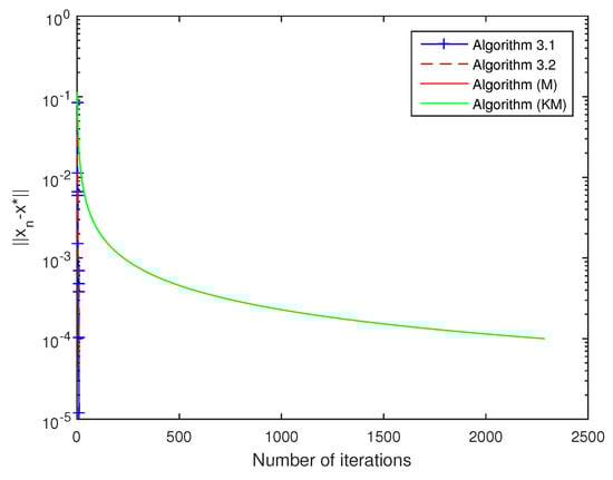
Figure 1. Comparison of all algorithms with $x_0=\frac{sin(-3t)}{100}$.

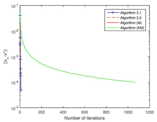
Figure 2. Comparison of all algorithms with $x_0=\frac{\left(sin\right(-3\ast t)+cos(-10\ast t\left)\right)}{300}$.

Example 2.

Assume that $A:{\mathbb{R}}^m\to {\mathbb{R}}^m$ is defined by $A\left(x\right)=Mx+q$ with $M=B{B}^T+S+D$, where S is an $m\times m$ skew-symmetric matrix, B is an $m\times m$ matrix, D is an $m\times m$ diagonal matrix, whose diagonal entries are positive (so M is positive definite), q is a vector in ${\mathbb{R}}^m$ and

$$C:=\{x\in {\mathbb{R}}^m:-5\le x_i\le 5,i=1,\cdots ,m\}.$$

Clearly, we can see that the operator A is monotone and Lipschitz continuous with a Lipschitz constant $L=\parallel M\parallel$. Given that $q=0$, the unique solution of the corresponding (VIP) is $\left\{0\right\}$.

We will compare Algorithm 3.1, Algorithm 3.2 with Tseng’s extragradient method (TEGM) [41], Inertial Tseng extragradient algorithm (ITEGM) of Thong and Hieu [33], subgradient extragradient method (SEGM) of Censor et al. [5]. We choose $\tau =\frac{0.9}{L}$ for all algorithm, ${\alpha }_n=\alpha =0.99\frac{\sqrt{1+8ϵ}-1-2ϵ}{2(1-ϵ)}$ where $ϵ=\frac{1-\lambda L}{1+\lambda L}$ for inertial Tseng extragradient algorithm. The starting points are $x_0={(1,1,\dots ,1)}^T\in {\mathbb{R}}^m.$

For experiment, all entries of B, S and D are generated randomly from a normal distribution with mean zero and unit variance. We use stopping rule $\parallel x_n-0\parallel <{10}^{-4}$ or Iter <= 1000 for all algorithms. The results are described in Table 2 and Figure 3 and Figure 4.

Table 2. Numerical results obtained by other algorithms.

Methods	m = 50			m = 100
	Sec.	Iter.	Error.	Sec.	Iter.	Error.
Algorithm 3.1	0.08	10	6.9882 × ${10}^{-5}$	0.14063	10	6.6947 × ${10}^{-5}$
Algorithm 3.2	0.078	8	9.0032 × ${10}^{-5}$	0.1	9	9.9385 × ${10}^{-5}$
TEGM	4.2438	1000	0.0849	9.4531	1000	0.2646
ITEGM	4.5188	1000	0.0790	9.6875	1000	0.2594
SEGM	4.3969	1000	0.0850	9.5156	1000	0.2647

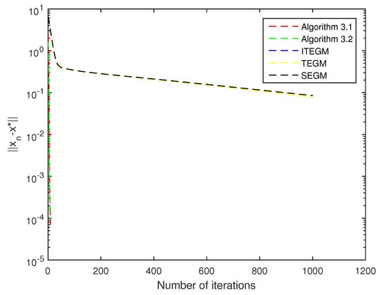
Figure 3. Comparison of all algorithms with $m=50$.

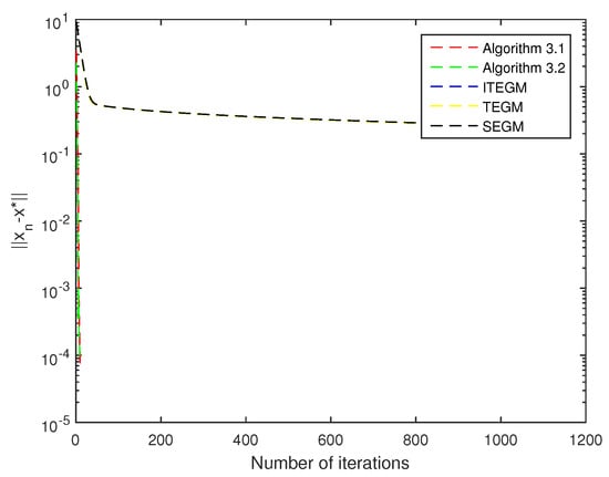
Figure 4. Comparison of all algorithms with $m=100$.

Table 1 and Table 2 and Figure 1, Figure 2, Figure 3 and Figure 4, give the errors of the Mainge’s algorithm [37] and Kraikaew and Saejung’s algorithm [40], Tseng’s extragradient method (TEGM) [41], Inertial Tseng extragradient algorithm (ITEGM) [33], subgradient extragradient method (SEGM) of Censor et al. [5] and Algorithms 3.1, 3.2 as well as their execution times. They show that Algorithms 3.1 and 3.2 are less time consuming and more accurate than those of Mainge [37], Kraikaew and Saejung [40], Tseng [41], Thong and Hieu [33] and Censor et al. [5].

5. Conclusions

In this study, we developed two new iterative algorithms for solving K-pseudomonotone variational inequality problems in the framework of real Hilbert spaces. We established some strong convergence theorems for our proposed algorithms under certain conditions. We proved via several numerical experiments that our proposed algorithms performs better in comparison than those of Mainge [37], Kraikaew and Saejung [40], Tseng [41], Thong and Hieu [33] and Censor et al. [5].

Data AvailabilityThe authors declare that all data relating to our results in this paper are available within the paper.

References

- Stampacchia, G. Formes bilineaires coercitives sur les ensembles convexes. C. R. Acad. Sci. 1964, 258, 4413–4416. [Google Scholar]
- Browder, F.E. The fixed point theory of multivalued mapping in topological vector spaces. Math. Ann. 1968, 177, 283–301. [Google Scholar] [CrossRef]
- Censor, Y.; Gibali, A.; Reich, S. The subgradient extragradient method for solving variational inequalities in Hilbert space. J. Optim. Theory Appl. 2011, 148, 318–335. [Google Scholar] [CrossRef] [PubMed]
- Censor, Y.; Gibali, A.; Reich, S. Strong convergence of subgradient extragradient methods for the variational inequality problem in Hilbert space. Optim. Methods Softw. 2011, 26, 827–845. [Google Scholar] [CrossRef]
- Censor, Y.; Gibali, A.; Reich, S. Algorithms for the split variational inequality problem. Numer. Algorithm 2012, 59, 301–323. [Google Scholar] [CrossRef]
- Censor, Y.; Gibali, A.; Reich, S. Extensions of Korpelevich’s extragradient method for the variational inequality problem in Euclidean space. Optimization 2012, 61, 1119–1132. [Google Scholar] [CrossRef]
- Gibali, A.; Shehu, Y. An efficient iterative method for finding common fixed point and variational inequalities in Hilbert spaces. Optimization 2019, 68, 13–32. [Google Scholar] [CrossRef]
- Gibali, A.; Ha, N.H.; Thuong, N.T.; Trang, T.H.; Vinh, N.T. Polyak’s gradient method for solving the split convex feasibility problem and its applications. J. Appl. Numer. Optim. 2019, 1, 145–156. [Google Scholar]
- Khan, A.R.; Ugwunnadi, G.C.; Makukula, Z.G.; Abbas, M. Strong convergence of inertial subgradient extragradient method for solving variational inequality in Banach space. Carpathian J. Math. 2019, 35, 327–338. [Google Scholar]
- Maingé, P.E. Projected subgradient techniques and viscosity for optimization with variational inequality constraints. Eur. J. Oper. Res. 2010, 205, 501–506. [Google Scholar] [CrossRef]
- Thong, D.V.; Vinh, N.T.; Cho, Y.J. Accelerated subgradient extragradient methods for variational inequality problems. J. Sci. Comput. 2019, 80, 1438–1462. [Google Scholar] [CrossRef]
- Wang, F.; Pham, H. On a new algorithm for solving variational inequality and fixed point problems. J. Nonlinear Var. Anal. 2019, 3, 225–233. [Google Scholar]
- Wang, L.; Yu, L.; Li, T. Parallel extragradient algorithms for a family of pseudomonotone equilibrium problems and fixed point problems of nonself-nonexpansive mappings in Hilbert space. J. Nonlinear Funct. Anal. 2020, 2020, 13. [Google Scholar]
- Alber, Y.I.; Iusem, A.N. Extension of subgradient techniques for nonsmooth optimization in Banach spaces. Set Valued Anal. 2001, 9, 315–335. [Google Scholar] [CrossRef]
- Xiu, N.H.; Zhang, J.Z. Some recent advances in projection-type methods for variational inequalities. J. Comput. Appl. Math. 2003, 152, 559–587. [Google Scholar] [CrossRef]
- Korpelevich, G.M. The extragradient method for finding saddle points and other problems. Ekon. Mat. Metod. 1976, 12, 747–756. [Google Scholar]
- Farouq, N.E. Pseudomonotone variational inequalities: Convergence of proximal methods. J. Optim. Theory Appl. 2001, 109, 311–326. [Google Scholar] [CrossRef]
- Hadjisavvas, N.; Schaible, S.; Wong, N.-C. Pseudomonotone operators: A survey of the theory and its applications. J. Optim. Theory Appl. 2012, 152, 1–20. [Google Scholar] [CrossRef]
- Kien, B.T.; Lee, G.M. An existence theorem for generalized variational inequalities with discontinuous and pseudomonotone operators. Nonlinear Anal. 2011, 74, 1495–1500. [Google Scholar] [CrossRef]
- Yao, J.-C. Variational inequalities with generalized monotone operators. Math. Oper. Res. 1994, 19, 691–705. [Google Scholar] [CrossRef]
- Karamardian, S. Complementarity problems over cones with monotone and pseudomonotone maps. J. Optim. Theory Appl. 1976, 18, 445–454. [Google Scholar] [CrossRef]
- Attouch, H.; Goudon, X.; Redont, P. The heavy ball with friction. I. The continuous dynamical system. Commun. Contemp. Math. 2000, 2, 1–34. [Google Scholar] [CrossRef]
- Attouch, H.; Czamecki, M.O. Asymptotic control and stabilization of nonlinear oscillators with non-isolated equilibria. J. Differ. Equ. 2002, 179, 278–310. [Google Scholar] [CrossRef]
- Alvarez, F.; Attouch, H. An inertial proximal method for maximal monotone operators via discretization of a nonlinear oscillator with damping. Set-Valued Anal. 2001, 9, 3–11. [Google Scholar] [CrossRef]
- Maingé, P.E. Inertial iterative process for fixed points of certain quasi-nonexpansive mappings. Set Valued Anal. 2007, 15, 67–69. [Google Scholar] [CrossRef]
- Maingé, P.E. Convergence theorems for inertial KM-type algorithms. J. Comput. Appl. Math. 2008, 219, 223–236. [Google Scholar] [CrossRef]
- Bot, R.I.; Csetnek, E.R.; Hendrich, C. Inertial Douglas-Rachford splitting for monotone inclusion problems. Appl. Math. Comput. 2015, 256, 472–487. [Google Scholar]
- Attouch, H.; Peypouquet, J.; Redont, P. A dynamical approach to an inertial forward-backward algorithm for convex minimization. SIAM J. Optim. 2014, 24, 232–256. [Google Scholar] [CrossRef]
- Chen, C.; Chan, R.H.; Ma, S.; Yang, J. Inertial proximal ADMM for linearly constrained separable convex optimization. SIAM J. Imaging Sci. 2015, 8, 2239–2267. [Google Scholar] [CrossRef]
- Bot, R.I.; Csetnek, E.R. A hybrid proximal-extragradient algorithm with inertial effects. Numer. Funct. Anal. Optim. 2015, 36, 951–963. [Google Scholar] [CrossRef]
- Bot, R.I.; Csetnek, E.R. An inertial forward-backward-forward primal-dual splitting algorithm for solving monotone inclusion problems. Numer. Algor. 2016, 71, 519–540. [Google Scholar] [CrossRef]
- Dong, L.Q.; Cho, Y.J.; Zhong, L.L.; Rassias, T.M. Inertial projection and contraction algorithms for variational inequalities. J. Glob. Optim. 2018, 70, 687–704. [Google Scholar] [CrossRef]
- Thong, D.V.; Hieu, D.V. Modified Tseng’s extragradient algorithms for variational inequality problems. J. Fixed Point Theory Appl. 2018, 20, 152. [Google Scholar] [CrossRef]
- Moudafi, A. Viscosity approximations methods for fixed point problems. J. Math. Anal. Appl. 2000, 241, 46–55. [Google Scholar] [CrossRef]
- Khan, S.H. A Picard-Mann hybrid iterative process. Fixed Point Theory Appl. 2013, 2013, 69. [Google Scholar] [CrossRef]
- Goebel, K.; Reich, S. Uniform Convexity, Hyperbolic Geometry and Nonexpansive Mappings; Marcel Dekker: New York, NY, USA; Basel, Switzerland, 1984. [Google Scholar]
- Maingé, P.E. A hybrid extragradient-viscosity method for monotone operators and fixed point problems. SIAM J. Control Optim. 2008, 47, 1499–1515. [Google Scholar] [CrossRef]
- Liu, L.S. Ishikawa and Mann iteration process with errors for nonlinear strongly accretive mappings in Banach spaces. J. Math. Anal. Appl. 1995, 194, 114–125. [Google Scholar] [CrossRef]
- Suantai, S.; Pholasa, N.; Cholamjiak, P. The modified inertial relaxed CQ algorithm for solving the split feasibility problems. J. Ind. Manag. Optim. 2018, 14, 1595–1615. [Google Scholar] [CrossRef]
- Kraikaew, R.; Saejung, S. Strong convergence of the Halpern subgradient extragradient method for solving variational inequalities in Hilbert spaces. J. Optim. Theory Appl. 2014, 163, 399–412. [Google Scholar] [CrossRef]
- Tseng, P. A modified forward-backward splitting method for maximal monotone mappings. SIAM J. Control Optim. 2000, 38, 431–446. [Google Scholar] [CrossRef]
© 2020 by the authors. Licensee MDPI, Basel, Switzerland. This article is an open access article distributed under the terms and conditions of the Creative Commons Attribution (CC BY) license (http://creativecommons.org/licenses/by/4.0/).