A Study Concerning Soft Computing Approaches for Stock Price Forecasting


Abstract
1. Introduction
2. Literature Review
2.1. Hidden Markov Model
2.2. Support Vector Machine
2.3. Artificial Neural Network
2.4. Discrete Wavelet Transform-Based Models
2.5. Empirical Mode Decomposition-Based Models
3. Data and Methods
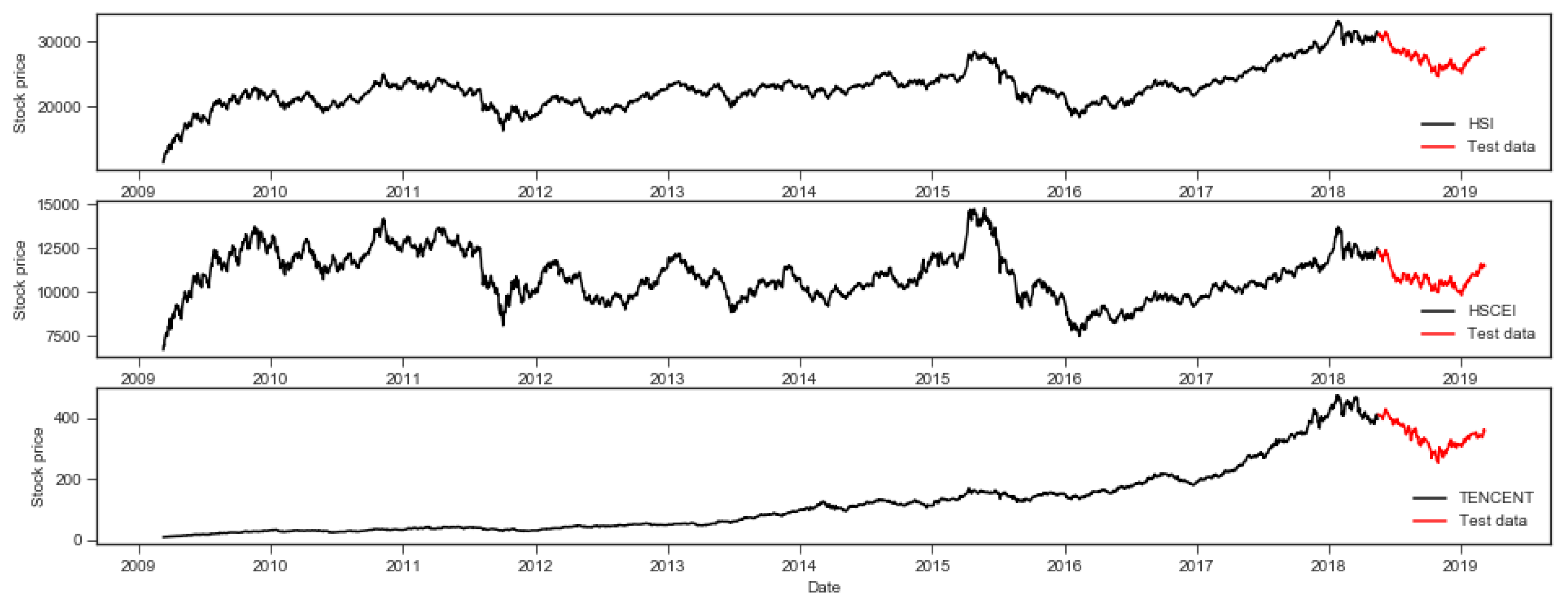
3.1. Data Sets
3.2. Comparison Criteria
3.3. HMM
3.4. SVM
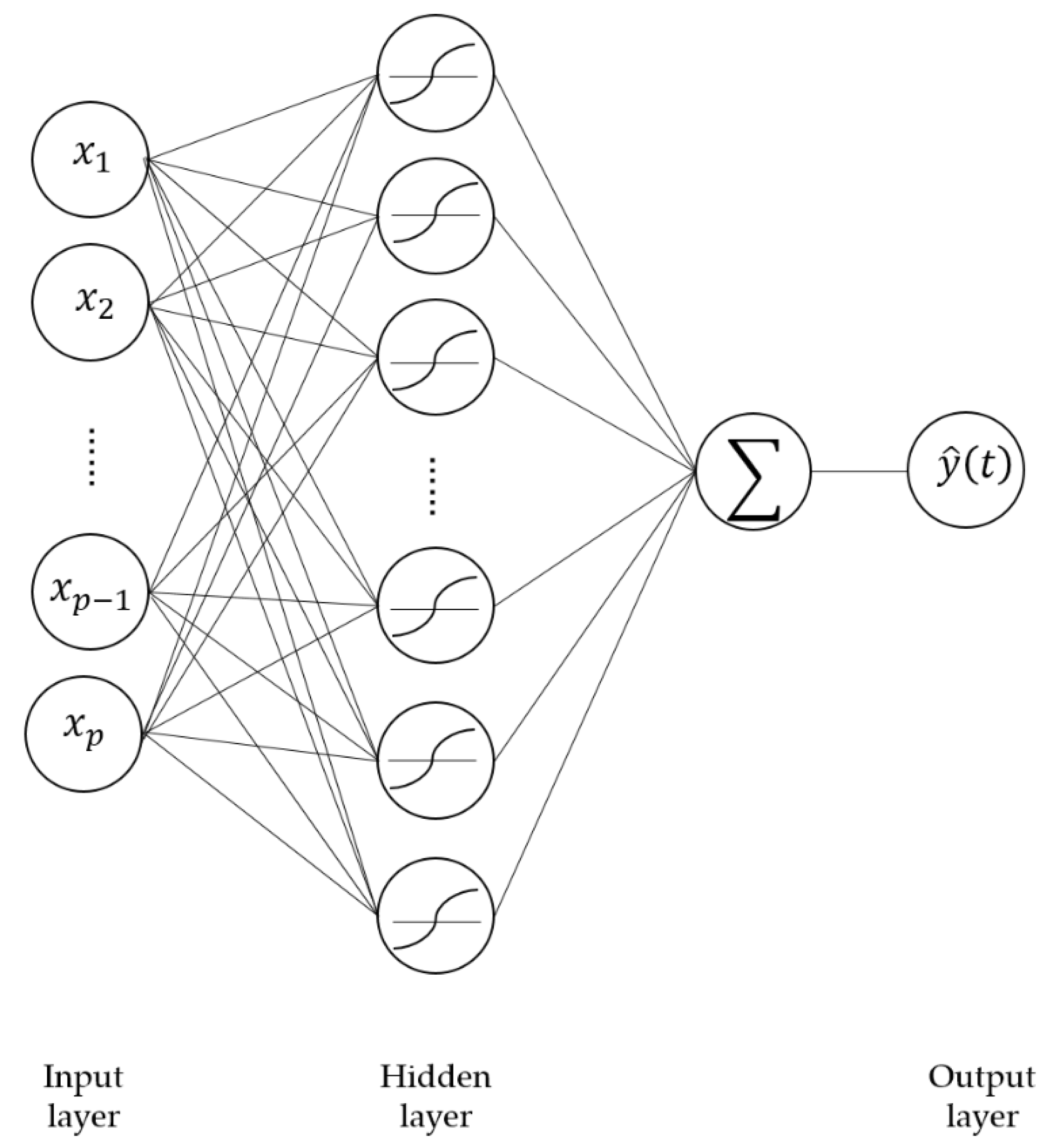
3.5. ANN
3.6. DWT
3.7. EMD
- (1)
- Identify all the local maxima and minima of .
- (2)
- Connect all the local maxima and local minima separately by the cubic spline to form the upper envelope line and lower envelope line .
- (3)
- Calculate the mean value of the upper and lower envelope .
- (4)
- Derive a new time-series by subtracting the mean envelope, .
- (5)
- If satisfies the properties of IMF [64]; then, is regarded as an IMF, and in step 1 is replaced with the new process Otherwise, substitute in step 1 by and repeat all of the above process.
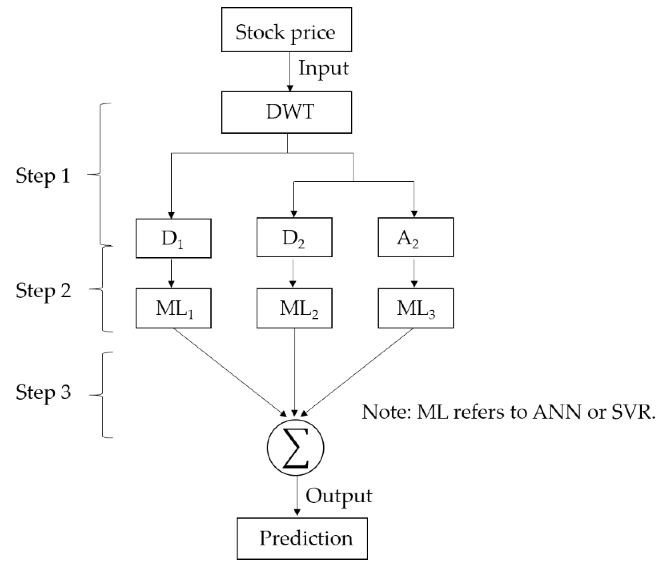
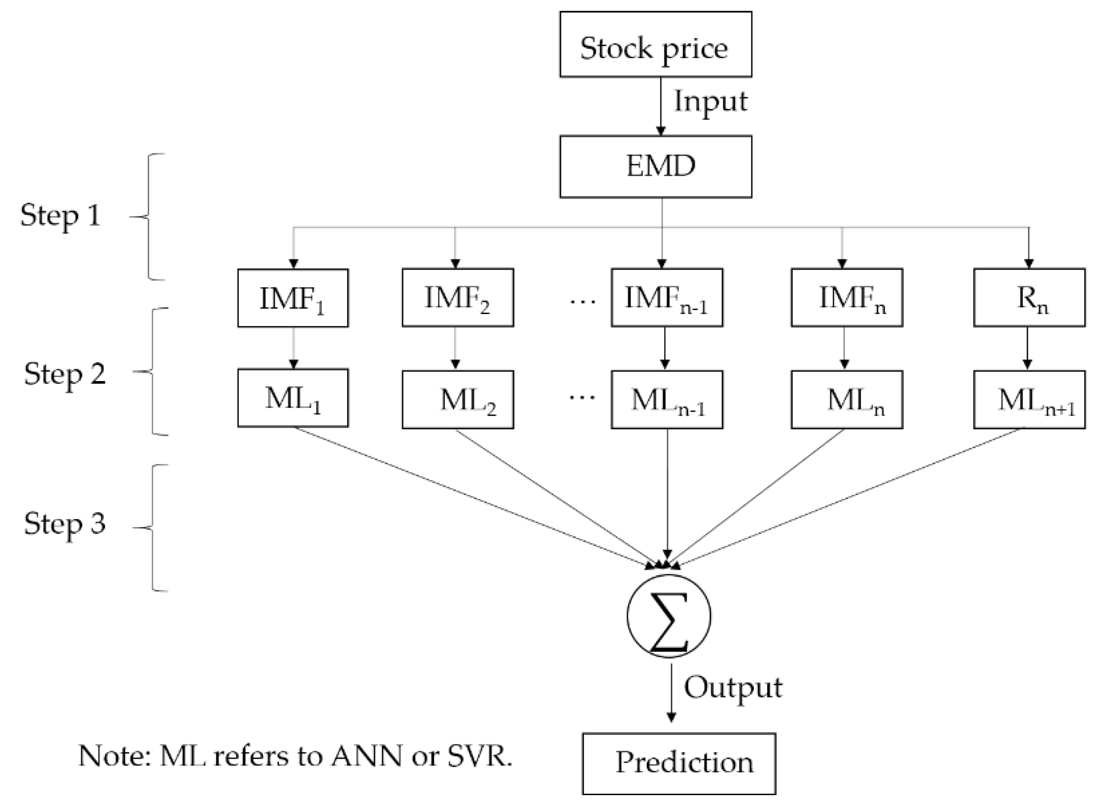
3.8. Overall Process of Hybrid Machine Learning Models
4. Experimental Results
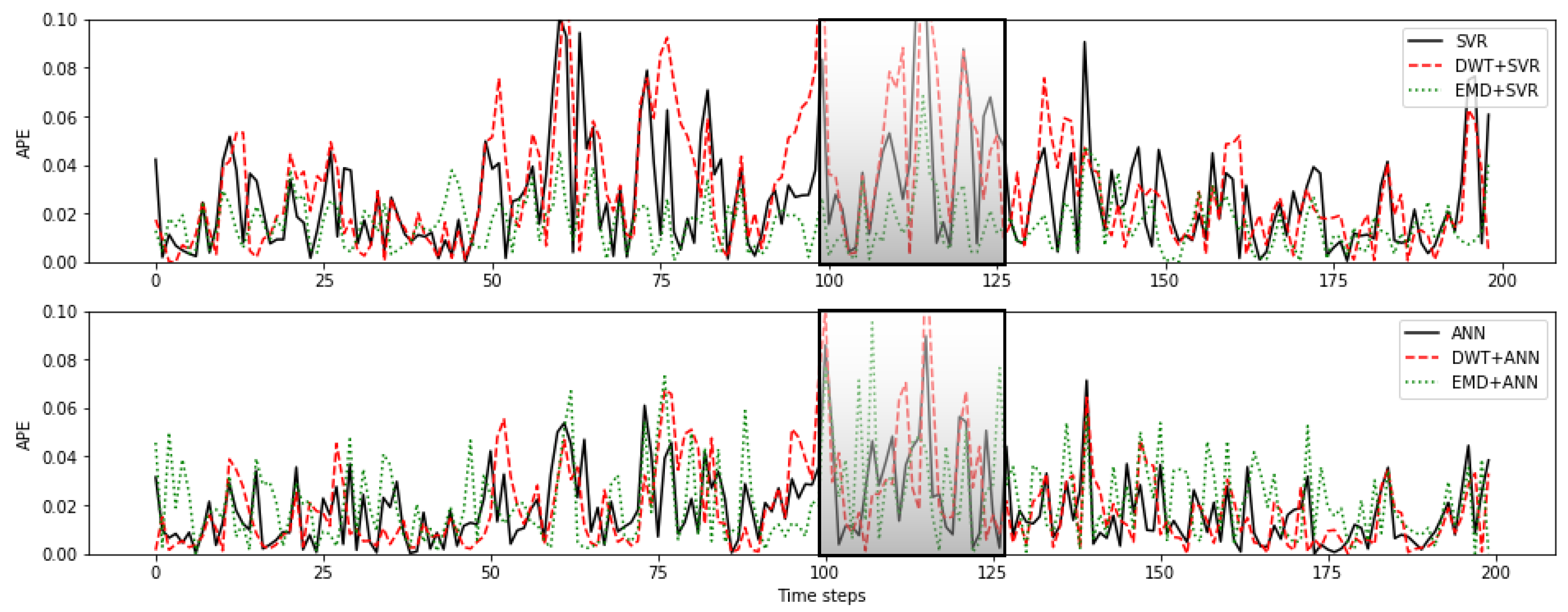
4.1. MAPE Comparison
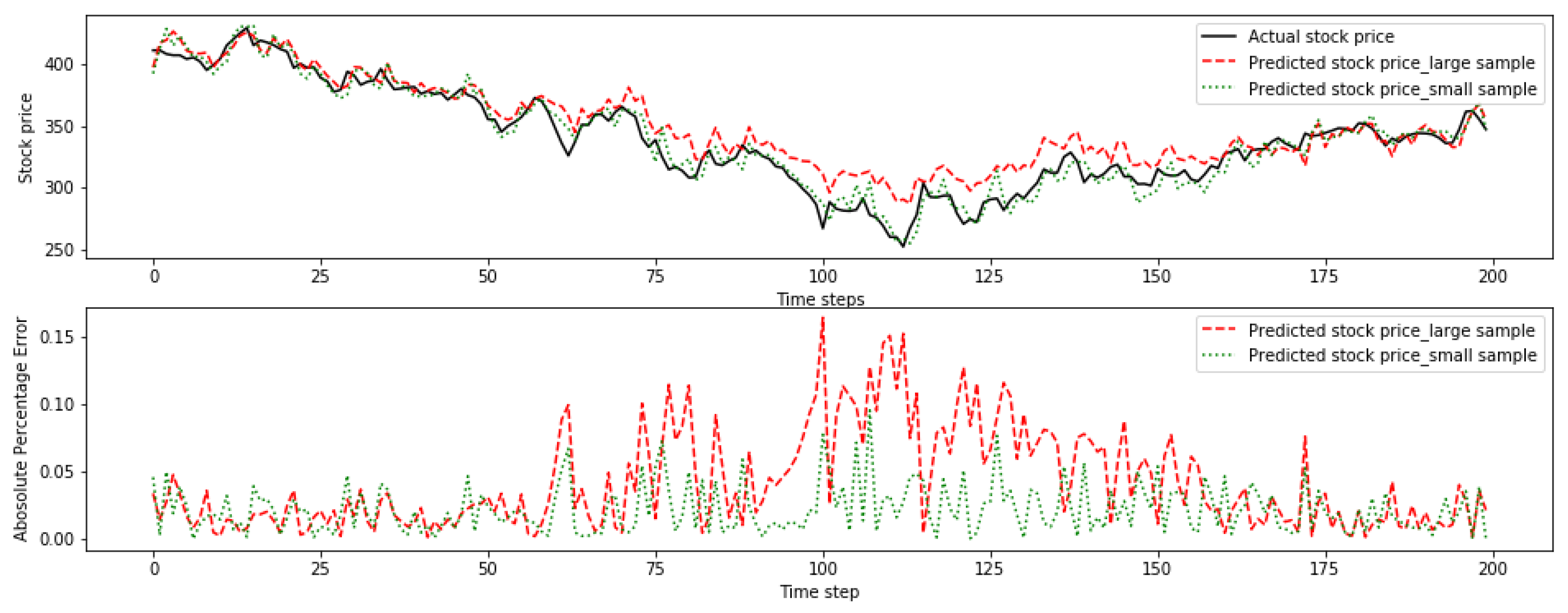
4.2. Sample Size Effect
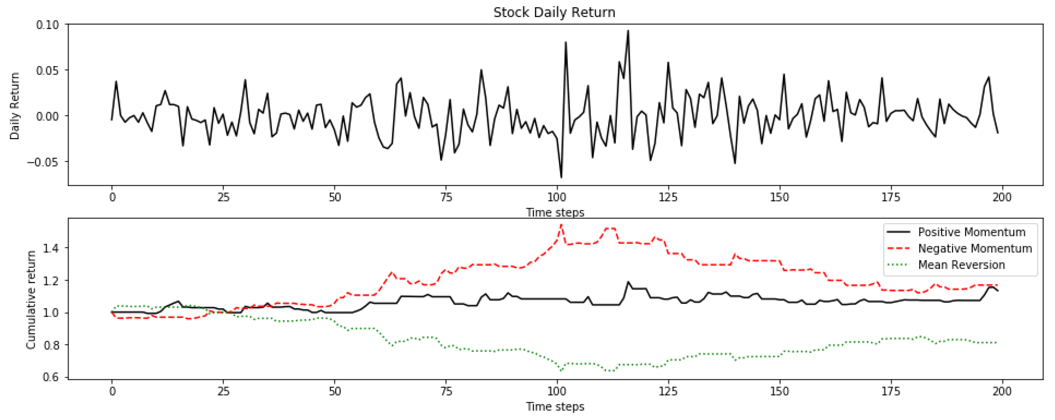
4.3. Momentum and Mean Reversion Stock Pattern Effect
5. Conclusions
Author Contributions
Acknowledgments
Conflicts of Interest
Abbreviations
| AIC | Akaike Information Criterion |
| ANFIS | Adaptive Neuro Fuzzy Inference System |
| ANN | Artificial Neural Network |
| APE | Absolute Percentage Error |
| AR | Autoregressive Model |
| ARCH | Autoregressive Conditional Heteroskedasticity Model |
| ARIMA | Autoregressive Integrated Moving Average |
| BDI | Baltic Dry Index |
| BP | Backpropagation |
| BPNN | Backpropagation Neural Network |
| CAPM | Capital Asset Pricing Model |
| DJIA | Down Jones Industrial Average |
| DWT | Discrete Wavelet Transform |
| EM | Expectation-Maximization Algorithm |
| EMD | Empirical Mode Decomposition |
| EMH | Efficient Market Hypothesis |
| GA | Genetic Algorithm |
| GMM | Gaussian Mixture Model |
| GRNN | General Regression Neural Network |
| HMM | Hidden Markov Model |
| HSCEI | Hong Seng China Enterprises Index |
| HSI | Hang Seng Index |
| IMF | Intrinsic Mode Function |
| LDA | Linear Discriminant Analysis |
| LS-SVR | Least Square Support Vector Regression |
| MAPE | Mean Absolute Percentage Error |
| MODWT | Maximum Overlap Discrete Wavelet Transform |
| ML | Machine Learning |
| NN | Neural Network |
| RBF | Radial Basis Function |
| RBFNN | Radial Basis Function Neural Network |
| S.D. | Standard Deviation |
| SVM | Support Vector Machine |
| SVR | Support Vector Regression |
References
- Malkiel, B.G. A Random Walk down Wall Street: Including a Life-Cycle Guide to Personal Investing, 7th ed.; WW Norton & Company: New York, NY, USA, 1999. [Google Scholar]
- Malkiel, B.G.; Fama, E.F. Efficient capital markets: A review of theory and empirical work. J. Financ. 1970, 25, 383–417. [Google Scholar] [CrossRef]
- Fama, E.F. Efficient capital markets: II. J. Financ. 1991, 46, 1575–1617. [Google Scholar] [CrossRef]
- Ramsey, J.B. Wavelets in economics and finance: Past and future. Stud. Nonlinear Dyn. Econom. 2002, 6, 1–27. [Google Scholar] [CrossRef]
- Atsalakis, G.S.; Valavanis, K.P. Forecasting stock market short-term trends using a neuro-fuzzy based methodology. Expert Syst. Appl. 2009, 36, 10696–10707. [Google Scholar] [CrossRef]
- Chollet, F. Deep Learning with Python, 1st ed.; Manning Publications Co.: Shelter Island, NY, USA, 2018. [Google Scholar]
- Vanstone, B.; Finnie, G. An empirical methodology for developing stockmarket trading systems using artificial neural networks. Expert Syst. Appl. 2009, 36, 6668–6680. [Google Scholar] [CrossRef]
- Zhong, X.; Enke, D. Forecasting daily stock market return using dimensionality reduction. Expert Syst. Appl. 2017, 67, 126–139. [Google Scholar] [CrossRef]
- Fabozzi, F.J.; Focardi, S.M.; Kolm, P.N. Quantitative Equity Investing: Techniques and Strategies, 1st ed.; John Wiley & Sons: Hoboken, NJ, USA, 2010. [Google Scholar]
- Cochrane, J.H. New Facts in Finance; Federal Reserve Bank of Chicago: Chicago, IL, USA, 1999; pp. 36–58. [Google Scholar]
- Devendra, K. Soft Computing: Techniques and Its Applications in Electrical Engineering; Springer: Berlin, Germany, 2008. [Google Scholar]
- Yin, S.; Jiang, Y.; Tian, Y.; Kaynak, O. A data-driven fuzzy information granulation approach for freight volume forecasting. IEEE Trans. Ind. Electron. 2016, 64, 1447–1456. [Google Scholar] [CrossRef]
- Jiang, Y.; Yin, S. Recent advances in key-performance-indicator oriented prognosis and diagnosis with a matlab toolbox: Db-kit. IEEE Trans. Ind. Inform. 2018, 15, 2849–2858. [Google Scholar] [CrossRef]
- Choudhary, A.; Upadhyay, K.; Tripathi, M. Soft computing applications in wind speed and power prediction for wind energy. In Proceedings of the 2012 IEEE Fifth Power India Conference, Murthal, India, 19–22 December 2012. [Google Scholar]
- Engle, R.F. Autoregressive conditional heteroscedasticity with estimates of the variance of United Kingdom inflation. Econom. J. Econom. Soc. 1982, 50, 987–1007. [Google Scholar] [CrossRef]
- Atsalakis, G.S.; Valavanis, K.P. Surveying stock market forecasting techniques-Part I: Conventional methods. J. Comput. Optim. Econ. Financ. 2010, 2, 45–92. [Google Scholar]
- De Luca, G.; Genton, M.G.; Loperfido, N. A skew-in-mean GARCH model for financial returns. In Skew-Elliptical Distributions and Their Applications: A Journey Beyond Normality; CRC/Chapman & Hall: Boca Rapton, FL, USA, 2004. [Google Scholar]
- Breiman, L. Statistical modeling: The two cultures. Stat. Sci. 2001, 16, 199–231. [Google Scholar] [CrossRef]
- Gerlein, E.A.; McGinnity, M.; Belatreche, A.; Coleman, S. Evaluating machine learning classification for financial trading: An empirical approach. Expert Syst. Appl. 2016, 54, 193–207. [Google Scholar] [CrossRef]
- Arnott, R.D.; Harvey, C.R.; Markowitz, H. A backtesting protocol in the era of machine learning. J. Financ. Data Sci. 2019, 1, 64–74. [Google Scholar] [CrossRef]
- Di Matteo, T. Multi-scaling in finance. Quant. Financ. 2007, 7, 21–36. [Google Scholar] [CrossRef]
- Yu, L.; Wang, S.; Lai, K.K. Forecasting crude oil price with an EMD-based neural network ensemble learning paradigm. Energy Econ. 2008, 30, 2623–2635. [Google Scholar] [CrossRef]
- Atsalakis, G.S.; Valavanis, K.P. Surveying stock market forecasting techniques–Part II: Soft computing methods. Expert Syst. Appl. 2009, 36, 5932–5941. [Google Scholar] [CrossRef]
- Bahrammirzaee, A. A comparative survey of artificial intelligence applications in finance: Artificial neural networks, expert system and hybrid intelligent systems. Neural Comput. Appl. 2010, 19, 1165–1195. [Google Scholar] [CrossRef]
- De Luca, G.; Genton, M.G.; Loperfido, N. A Multivariate Skew-Garch Model. In Advances in Econometrics: Econometric Analysis of Economic and Financial Time Series; Part A (Special volume in honor of Robert Engle and Clive Granger, the 2003 Winners of the Nobel Prize in Economics); Terrell, D., Ed.; Elsevier: Oxford, UK, 2006. [Google Scholar]
- Hassan, M.R.; Nath, B. Stock market forecasting using hidden Markov model: A new approach. In Proceedings of the 5th International Conference on Intelligent Systems Design and Applications (ISDA’05), Warsaw, Poland, 8–10 September 2005. [Google Scholar]
- Hassan, M.R. A combination of hidden Markov model and fuzzy model for stock market forecasting. Neurocomputing 2009, 72, 3439–3446. [Google Scholar] [CrossRef]
- Hassan, M.R.; Nath, B.; Kirley, M. A fusion model of HMM, ANN and GA for stock market forecasting. Expert Syst. Appl. 2007, 33, 171–180. [Google Scholar] [CrossRef]
- Gupta, A.; Dhingra, B. Stock market prediction using hidden markov models. In Proceedings of the 2012 Students Conference on Engineering and Systems, Allahabad, India, 16–18 March 2012. [Google Scholar]
- Zhang, X.; Li, Y.; Wang, S.; Fang, B.; Philip, S.Y. Enhancing stock market prediction with extended coupled hidden Markov model over multi-sourced data. Knowl. Inf. Syst. 2018, 61, 1071–1090. [Google Scholar] [CrossRef]
- Schmidt, M. Identifying speaker with support vector networks. In Proceedings of the Interface ’96 Sydney, Sydney, Australia, 9–13 December 1996. [Google Scholar]
- Vapnik, V. The Nature of Statistical Learning Theory, 2nd ed.; Springer Science & Business Media: New York, NY, USA, 2013. [Google Scholar]
- Kim, K. Financial time series forecasting using support vector machines. Neurocomputing 2003, 55, 307–319. [Google Scholar] [CrossRef]
- Tay, F.E.; Cao, L. Application of support vector machines in financial time series forecasting. Omega 2001, 29, 309–317. [Google Scholar] [CrossRef]
- Huang, W.; Nakamori, Y.; Wang, S. Forecasting stock market movement direction with support vector machine. Comput. Oper. Res. 2005, 32, 2513–2522. [Google Scholar] [CrossRef]
- Henrique, B.M.; Sobreiro, V.A.; Kimura, H. Stock price prediction using support vector regression on daily and up to the minute prices. J. Financ. Data Sci. 2018, 4, 183–201. [Google Scholar] [CrossRef]
- Rustam, Z.; Kintandani, P. Application of Support Vector Regression in Indonesian Stock Price Prediction with Feature Selection Using Particle Swarm Optimization. Model. Simul. Eng. 2019, 2019. [Google Scholar] [CrossRef]
- Lee, M. Using support vector machine with a hybrid feature selection method to the stock trend prediction. Expert Syst. Appl. 2009, 36, 10896–10904. [Google Scholar] [CrossRef]
- Zhang, G.; Patuwo, B.E.; Hu, M.Y. Forecasting with artificial neural networks: The state of the art. Int. J. 1998, 14, 35–62. [Google Scholar]
- White, H. Economic prediction using neural networks: The case of IBM daily stock returns. In Proceedings of the IEEE 1988 International Conference on Neural Networks, San Diego, CA, USA, 24–27 July 1988. [Google Scholar]
- Kimoto, T.; Asakawa, K.; Yoda, M.; Takeoka, M. Stock market prediction system with modular neural networks. In Proceedings of the IEEE International Joint Con-ference on Neural Networks, San Diego, CA, USA, 17–21 June 1990. [Google Scholar]
- Qiu, M.; Song, Y. Predicting the direction of stock market index movement using an optimized artificial neural network model. PLoS ONE 2016, 11, e0155133. [Google Scholar] [CrossRef]
- Kara, Y.; Boyacioglu, M.A.; Baykan, Ö.K. Predicting direction of stock price index movement using artificial neural networks and support vector machines: The sample of the Istanbul Stock Exchange. Expert Syst. Appl. 2011, 38, 5311–5319. [Google Scholar] [CrossRef]
- Cao, Q.; Leggio, K.B.; Schniederjans, M.J. A comparison between Fama and French’s model and artificial neural networks in predicting the Chinese stock market. Comput. Oper. Res. 2005, 32, 2499–2512. [Google Scholar] [CrossRef]
- Song, Y.; Zhou, Y.; Han, R. Neural networks for stock price prediction. arXiv 2018, arXiv:1805.11317. [Google Scholar]
- Lawrence, S.; Giles, C.L.; Tsoi, A.C. Lessons in neural network training: Overfitting may be harder than expected. In Proceedings of the Fourteenth National Conference on Artificial Intelligence and Ninth Innovative Applications of Artificial Intelligence Conference, AAAI 97, IAAI 97, Providence, Rhode Island, 27–31 July 1997. [Google Scholar]
- Adebiyi, A.A.; Adewumi, A.O.; Ayo, C.K. Comparison of ARIMA and artificial neural networks models for stock price prediction. J. Appl. Math. 2014, 2014, 1–7. [Google Scholar] [CrossRef]
- Han, B. Framelets and Wavelets: Algorithms, Analysis, and Applications, 1st ed.; Birkhäuser: Basel, Switzerland, 2018. [Google Scholar]
- Mallat, S. Wavelet Tour of Signal Processing, 3rd ed.; Academic: New York, NY, USA, 2008. [Google Scholar]
- Chui, C.K. An Introduction to Wavelets, 1st ed.; Academic Press: San Diego, CA, USA, 2016. [Google Scholar]
- Daubechies, I. Ten Lectures on Wavelets; Siam: Philadelphia, PA, USA, 1992. [Google Scholar]
- Han, B.; Zhuang, X. Matrix extension with symmetry and its application to symmetric orthonormal multiwavelets. Siam J. Math. Anal. 2010, 42, 2297–2317. [Google Scholar] [CrossRef]
- Zhuang, X. Digital affine shear transforms: Fast realization and applications in image/video processing. Siam J. Imaging Sci. 2016, 9, 1437–1466. [Google Scholar] [CrossRef]
- Gurley, K.; Kareem, A. Applications of wavelet transforms in earthquake, wind and ocean engineering. Eng. Struct. 1999, 21, 149–167. [Google Scholar]
- Gençay, R.; Selçuk, F.; Whitcher, B. Scaling properties of foreign exchange volatility. Phys. A Stat. Mech. Appl. 2001, 289, 249–266. [Google Scholar] [CrossRef]
- Lahmiri, S. Wavelet low-and high-frequency components as features for predicting stock prices with backpropagation neural networks. J. King Saud Univ. Comput. Inf. Sci. 2014, 26, 218–227. [Google Scholar] [CrossRef]
- Li, J.; Shi, Z.; Li, X. Genetic programming with wavelet-based indicators for financial forecasting. Trans. Inst. Meas. Control 2006, 28, 285–297. [Google Scholar] [CrossRef]
- Hsieh, T.; Hsiao, H.; Yeh, W. Forecasting stock markets using wavelet transforms and recurrent neural networks: An integrated system based on artificial bee colony algorithm. Appl. Soft Comput. 2011, 11, 2510–2525. [Google Scholar] [CrossRef]
- Wang, J.; Wang, J.; Zhang, Z.; Guo, S. Forecasting stock indices with back propagation neural network. Expert Syst. Appl. 2011, 38, 14346–14355. [Google Scholar] [CrossRef]
- Jothimani, D.; Shankar, R.; Yadav, S.S. Discrete wavelet transform-based prediction of stock index: A study on National Stock Exchange Fifty index. J. Financ. Manag. Anal. 2015, 28, 35–49. [Google Scholar]
- Chandar, S.K.; Sumathi, M.; Sivanandam, S. Prediction of stock market price using hybrid of wavelet transform and artificial neural network. Indian J. Sci. Technol. 2016, 9, 1–5. [Google Scholar] [CrossRef]
- Khandelwal, I.; Adhikari, R.; Verma, G. Time series forecasting using hybrid ARIMA and ANN models based on DWT decomposition. Procedia Comput. Sci. 2015, 48, 173–179. [Google Scholar] [CrossRef]
- Huang, N.E.; Shen, Z.; Long, S.R.; Wu, M.C.; Shih, H.H.; Zheng, Q.; Yen, N.; Tung, C.C.; Liu, H.H. The empirical mode decomposition and the Hilbert spectrum for nonlinear and non-stationary time series analysis. Proc. R. Soc. Lond. Ser. A Math. Phys. Eng. Sci. 1998, 454, 903–995. [Google Scholar] [CrossRef]
- Huang, N.E.; Wu, Z. A review on Hilbert-Huang transform: Method and its applications to geophysical studies. Rev. Geophys. 2008, 46. [Google Scholar] [CrossRef]
- Wei, L. A hybrid ANFIS model based on empirical mode decomposition for stock time series forecasting. Appl. Soft Comput. 2016, 42, 368–376. [Google Scholar] [CrossRef]
- Drakakis, K. Empirical mode decomposition of financial data. Int. Math. Forum 2008, 3, 1191–1202. [Google Scholar]
- Nava, N.; Di Matteo, T.; Aste, T. Financial time series forecasting using empirical mode decomposition and support vector regression. Risks 2018, 6, 7. [Google Scholar] [CrossRef]
- Cheng, C.; Wei, L. A novel time-series model based on empirical mode decomposition for forecasting TAIEX. Econ. Model. 2014, 36, 136–141. [Google Scholar] [CrossRef]
- Lin, C.; Chiu, S.; Lin, T. Empirical mode decomposition–based least squares support vector regression for foreign exchange rate forecasting. Econ. Model. 2012, 29, 2583–2590. [Google Scholar] [CrossRef]
- Zeng, Q.; Qu, C. An approach for Baltic Dry Index analysis based on empirical mode decomposition. Marit. Policy Manag. 2014, 41, 224–240. [Google Scholar] [CrossRef]
- Yu, H.; Liu, H. Improved stock market prediction by combining support vector machine and empirical mode decomposition. In Proceedings of the 2012 Fifth International Symposium on Computational Intelligence and Design, Hangzhou, China, 28–29 October 2012. [Google Scholar]
- Peiro, A. Skewness in financial returns. J. Bank. Financ. 1999, 23, 847–862. [Google Scholar] [CrossRef]
- Shcherbakov, M.V.; Brebels, A.; Shcherbakova, N.L.; Tyukov, A.P.; Janovsky, T.A.; Kamaev, V.A. A survey of forecast error measures. World Appl. Sci. J. 2013, 24, 171–176. [Google Scholar]
- Willmott, C.J.; Matsuura, K. Advantages of the mean absolute error (MAE) over the root mean square error (RMSE) in assessing average model performance. Clim. Res. 2005, 30, 79–82. [Google Scholar] [CrossRef]
- Sakamoto, Y.; Ishiguro, M.; Kitagawa, G. Akaike Information Criterion Statistics; KTK Scientific Publishers: Dordrecht, The Netherlands, 1986. [Google Scholar]
- Martin, J.H.; Jurafsky, D. Speech and Language Processing: An Introduction to Natural Language Processing, Computational Linguistics, and Speech Recognition; Pearson/Prentice Hall: Upper Saddle River, NJ, USA, 2009. [Google Scholar]
- Smola, A.J.; Schölkopf, B. A tutorial on support vector regression. Stat. Comput. 2004, 14, 199–222. [Google Scholar] [CrossRef]
- Madge, S.; Bhatt, S. Predicting Stock Price Direction Using Support Vector Machines; Independent Work Report Spring; Princeton University: Princeton, NJ, USA, 2015. [Google Scholar]
- Sheela, K.G.; Deepa, S.N. Review on methods to fix number of hidden neurons in neural networks. Math. Probl. Eng. 2013, 2013. [Google Scholar] [CrossRef]
- Subasi, A. EEG signal classification using wavelet feature extraction and a mixture of expert model. Expert Syst. Appl. 2007, 32, 1084–1093. [Google Scholar] [CrossRef]
- Balvers, R.; Wu, Y.; Gilliland, E. Mean reversion across national stock markets and parametric contrarian investment strategies. J. Financ. 2000, 55, 745–772. [Google Scholar] [CrossRef]
- Fama, E.F.; French, K.R. Size, value, and momentum in international stock returns. J. Financ. Econ. 2012, 105, 457–472. [Google Scholar] [CrossRef]
- Bai, L.; Yan, S.; Zheng, X.; Chen, B.M. Market turning points forecasting using wavelet analysis. Phys. A Stat. Mech. Appl. 2015, 437, 184–197. [Google Scholar] [CrossRef]


| Article | Stock Market | Input Variables | Training Method | Comparative Studies | Best Model |
|---|---|---|---|---|---|
| [26] | - | Opening, high, low and closing price | HMM | ANN | Similar performance |
| [28] | USA | Opening, high, low and closing price | ANN-HMM-GA | ARIMA | Similar performance |
| [27] | - | Opening, high, low and closing price | HMM-Fuzzy | HMM, HMM-ANN-GA, ARIMA and ANN | HMM-Fuzzy |
| [29] | USA | Fractional change, fractional high and low | Maximum a Posterior HMM | HMM-Fuzzy, ARIMA and ANN | HMM |
| [30] | China | Open, high, low and closing price; news articles | Extended coupled HMM | SVM, TeSIA, CMT, ECHMM-NE, ECHMM-NC, ECHMM | ECHMM |
| Article | Stock Market | Input Variables | Training Method | Comparative Studies | Best Model |
|---|---|---|---|---|---|
| [34] | USA | Daily closing price of five future contracts | SVM | BPNN | SVM |
| [33] | Korea | 12 technical indicators | SVM | ANN and CBR | SVM |
| [35] | Japan | Weekly price of S&P500 Index and USD/Yen exchange rate | SVM | LDA, QDA, EPNN | SVM |
| [38] | USA | 29 technical indicators and lagged index price | SVM | BPNN | SVM |
| [37] | Indonesia | 14 technical indicators | Particle swarm optimization-SVR | - | - |
| [36] | Brazil, USA and China | 5 technical indicators for daily and 1-minute price | SVR | Random walk model | SVR |
| Article | Stock Market | Input Variables | Training Method | Comparative Studies | Best Model |
|---|---|---|---|---|---|
| [40] | USA | Daily stock return | NN | - | Over-optimistic |
| [41] | Japan | Technical indicators and economic indexes | NN | Multiple regression analysis | NN |
| [44] | China | Daily closing price; quarterly book value; common share outstanding | ANN | CAPM, Fama and Frech’s 3 factor model | ANN |
| [43] | Turkey | 10 technical indicators | ANN | SVM | ANN |
| [47] | USA | Daily opening, high, low and closing price; trading volume | ANN | ARIMA | ANN |
| [42] | Japan | Technical indicators | GA-ANN | - | - |
| [45] | China | Weekly close price | BPNN | RBF, GRNN, SVR, LS-SVR | BPNN |
| Article | Stock Market | Input Variables | Training Method | Comparative Studies | Best Model |
|---|---|---|---|---|---|
| [62] | - | Weekly exchange rate GBP/USD | DWT-ANN/ARIMA | ARIMA, ANN and Zhang′s hybrid model | DWT-ANN/ARIMA |
| [60] | India | Weekly closing price | MODWT-ANN/SVR | ANN, SVR | MODWT-ANN/SVR |
| [56] | USA | Minute-in-day closing price | DWT-BPNN | ARMA, Random walk model | DWT-BPNN |
| [59] | China | Monthly closing price | DWT-BPNN | BPNN | DWT-BPNN |
| [58] | Taiwan, USA, UK, Japan | 10 technical indicators | DWT-ABC-RNN | DWT-BP-ANN, BNN | DWT-ABC-RNN |
| [57] | USA | 9 technical indicators | DWT-FGP | - | - |
| Article | Stock Market | Input Variables | Training Method | Comparative Studies | Best Model |
|---|---|---|---|---|---|
| [22] | USA, UK | Daily crude oil spot price | EMD + ARIMA + ALNN; EMD-FNN-ALNN; EMD-ARIMA-Average | ARIMA, FNN | EMD - FNN - ALNN |
| [71] | China | Closing price | EMD-SVM | SVM | EMD-SVM |
| [69] | - | Daily exchange rate USD/NTD, JPY/NTD and RMB/NTD | EMD-LSSVR | EMD-ARIMA, LSSVR, ARIMA | EMD-SVR |
| [68] | Taiwan | Closing price | EMD-SVR | AR, SVR | EMD-SVR |
| [65] | Taiwan, HK | Closing price | EMD-ANFIS | SVR, AR, ANFIS | EMD-ANFIS |
| [67] | USA | Intraday price | EMD-SVR | ARIMA, Directed SVR, Recursive SVR | EMD-SVR |
| Statistics 1 | Hang Seng Index | Hang Seng China Enterprises Index | Tencent |
|---|---|---|---|
| Mean () | 0.05% | 0.04% | 0.19% |
| Standard Deviation () | 1.24% | 1.54% | 2.07% |
| Skewness () | 0.01 | 0.10 | 0.14 |
| Kurtosis () | 2.51 | 1.98 | 2.04 |
| Methodology | Hang Seng Index | Hang Seng China Enterprises Index | Tencent | |||
|---|---|---|---|---|---|---|
| MAPE (%) | Rank | MAPE (%) | Rank | MAPE (%) | Rank | |
| Benchmark S. D. | 1.24 | - | 1.54 | - | 2.07 | - |
| Random walk | 0.97 | - | 1.13 | - | 1.68 | - |
| HMM | 1.42 | 4 | 1.27 | 3 | 2.41 | 4 |
| SVR | 1.69 | 6 | 1.86 | 6 | 2.70 | 5 |
| DWT - SVR | 1.85 | 7 | 2.04 | 7 | 3.10 | 7 |
| EMD - SVR | 1.45 | 5 | 1.57 | 5 | 2.60 | 6 |
| ANN | 1.12 | 2 | 1.04 | 1 | 1.81 | 1 |
| DWT - ANN | 1.11 | 1 | 1.20 | 2 | 1.83 | 2 |
| EMD - ANN | 1.21 | 3 | 1.35 | 4 | 2.25 1 | 3 |
© 2019 by the authors. Licensee MDPI, Basel, Switzerland. This article is an open access article distributed under the terms and conditions of the Creative Commons Attribution (CC BY) license (http://creativecommons.org/licenses/by/4.0/).
Share and Cite
Shi, C.; Zhuang, X. A Study Concerning Soft Computing Approaches for Stock Price Forecasting. Axioms 2019, 8, 116. https://doi.org/10.3390/axioms8040116
Shi C, Zhuang X. A Study Concerning Soft Computing Approaches for Stock Price Forecasting. Axioms. 2019; 8(4):116. https://doi.org/10.3390/axioms8040116
Chicago/Turabian StyleShi, Chao, and Xiaosheng Zhuang. 2019. "A Study Concerning Soft Computing Approaches for Stock Price Forecasting" Axioms 8, no. 4: 116. https://doi.org/10.3390/axioms8040116
APA StyleShi, C., & Zhuang, X. (2019). A Study Concerning Soft Computing Approaches for Stock Price Forecasting. Axioms, 8(4), 116. https://doi.org/10.3390/axioms8040116