GRSA Enhanced for Protein Folding Problem in the Case of Peptides

 ,
,  ,
, 
Abstract
1. Introduction
2. Background
- To design the physical code that aims to determine the interatomic forces of the protein structure for a given amino acid sequence.
- To solve the computational problem of designing an algorithm to predict the native structure from a given amino acid sequence.
- To perform an algorithm for the folding process by nature, which rapidly finds the routes or pathways from an initial solution to the NS or functional structure.
2.1. Computational Methods in PFP
2.2. Simulated Annealing
| Algorithm 1 Classical Simulated Annealing. |
| 1: SA (, , , ) |
| 2: |
| 3: |
| 4: while do |
| 5: while do |
| 6: |
| 7: |
| 8: if then |
| 9: |
| 10: else if then |
| 11: |
| 12: end |
| 13: end |
| 14: |
| 15: end |
| 16: end |
2.3. Chemical Reaction Optimization
- Unimolecular collisions: When the molecule hits the wall of the container.
- Intermolecular collision: When a molecule collides with other molecules.
- Unimolecular collision (low energy collisions). In this group, we find two reactions:
- On-wall ineffective collision is established as follows [39]:“It represents the situation when a molecule collides with a wall of the container and then bounces away remaining in one single unit”.In GRSA2, the current solution is changed by a new solution obtained by a perturbation function. This operation is equivalent to the classical SA perturbation. Thus, the complexity of GRSA2 is not modified. This operation is implemented in line seven of Algorithm 3, which calls the function soft perturbation or Algorithm 2, explained in Section 4. As we will see, this operation does not add complexity to the classical SA.
- Decomposition. In this case, a molecule (solution) hits a wall and then is divided into several parts. In the GRSA2 algorithm, decomposition is a perturbation operation that generates two new solutions from the current solution. This perturbation is implemented in GRSA2 in lines sixth and seven of Algorithms 2 and 3, respectively. Again, to include this operation in SA for obtaining GRSA2 does not increase the complexity of the new algorithm.
- Intermolecular collision (high energy collisions). This collision has the next elementary reactions:
- Intermolecular ineffective collision. These kinds of reactions occur when multiple molecules collide with each other and then bounce away. The number of molecules remains the same.
- Synthesis. In this reaction, several molecules are fused into a single one.
2.4. Analytical Tuning Method
3. Ab Initio Definition
3.1. Ab Initio Problem in PFP
- Given a sequence of amino acids; , which represents the primary structure of a protein with a set of dihedral angles , and an energy function which represents the free energy or Gibbs energy (G).
- Find the native structure of the protein, such that represents the minimum energy value, where the optimal solution defines the best three-dimensional configuration. The PFP variables are the set of dihedral angles.
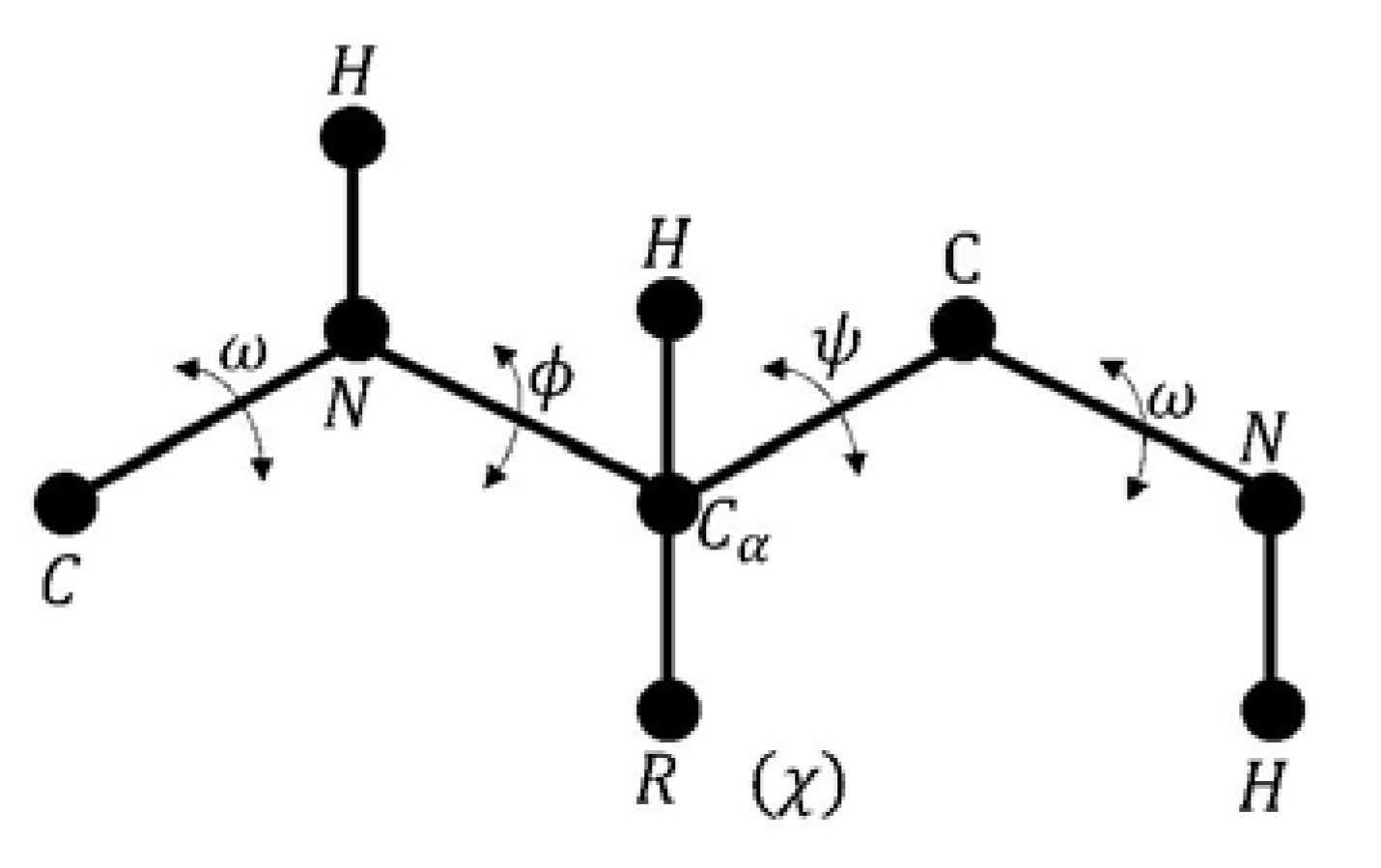
- Phi is the angle between the amino group and the alpha carbon.
- Psi is the angle between the alpha carbon and the carboxyl group.
- Omega is defined for each two consecutive amino acids.
- Chi is defined between the two planes conformed by two consecutive carbon atoms in the radical group.
3.2. Force Field
- is the distance in between the atoms and .
- and are the parameters of the empirical potentials.
- and are the partial charges on the atoms and , respectively.
- is the dielectric constant, which is usually set to .
- 332 is a factor used to obtain the energy in kcal/mol.
- is the energetic torsion barrier of rotation about the bond .
- is the multiplicity of the torsion angle .
4. An Enhancement of Golden Ratio Simulated Annealing
4.1. The Enhancement of GRSA
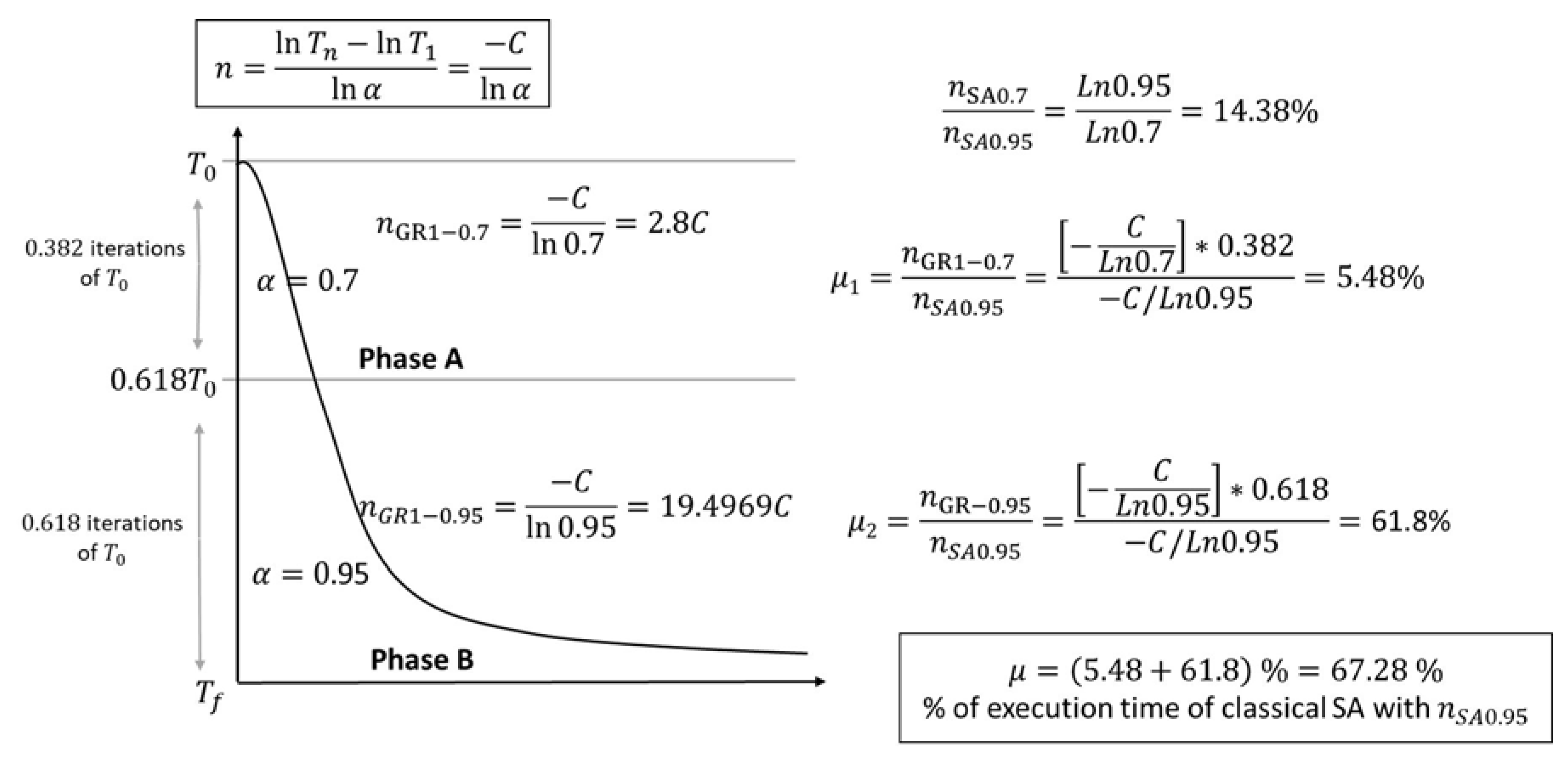
- GRSA with one cut-off temperature:
- The processing time of phase A is multiplied by the fraction of iterations where this phase is executed . Let be the proportion of time of phase A concerning the normal execution time of SA (); as is shown in Figure 2, of .
- The processing time of phase B is given by . Now, the time proportion of phase B for the normal execution of SA is of .
- The total proportion of GRSA processing time compared to SA is .
- GRSA with two or more cut-off temperatures
- Phase A is the same process as case 1 (with ) and uses of .
- Phase B is divided into nGolden sections. For instance, if nGolden equals 2, phase B is divided into two subphases. The new values for the next subsections can be again 0.7 and 0.95 for the next subphases. In other words, each time a subdivision is made, the last subphase will have a new parameter equal to 0.95. The division process continues until nGolden parameter is reached. When nGolden equals 2, the two new subphases (with and ) will have of the execution time of phase B. The proportion of the total processing time (time of phase A plus time of new subphases generated from B) will be of the execution time of SA.
- When nGolden is increased, a reduction of the time is obtained.
- The alpha values can be changed in several ways. Instead of using the last numbers (0.7, 0.95) to divide the subsections, a linear or exponential function for the alphas can be used. In our case, the linear approach was used [14], which gives similar reductions to those previously presented. Experimentation reveals that, in general, a nGolden value lower or equal to five gives good results in the case of peptides.
4.2. Soft Perturbation in GRSA
| Algorithm 2 Soft perturbation. |
| 1: SoftPertubation () |
| 2: |
| 3: if then |
| 4: Randomly select one particle |
| 5: if then |
| 6: |
| 7: else if |
| 8: |
| 9: end |
| 10: end |
| 11: end |
| Algorithm 3 GRSA2. |
| 1: GRSA2 (, , , E, S, , KE, EP nGolden) |
| 2: |
| 3: |
| 4: while do |
| 5: |
| 6: while do |
| 7: |
| 8: EP = Enew |
| 9: if then |
| 10: |
| 11: KE = ((Eold+KE)-EP)*random [0, 1] |
| 12: end if |
| 13: end while |
| 14: if then |
| 15: |
| 16: if then |
| 17: (the algorithm is stopped) |
| 18: end if |
| 19: end if |
| 20: if then |
| 21: |
| 22: |
| 23: else |
| 24: |
| 25: end if |
| 26: end while |
| 27: end |
5. Results
5.1. Experimental Description
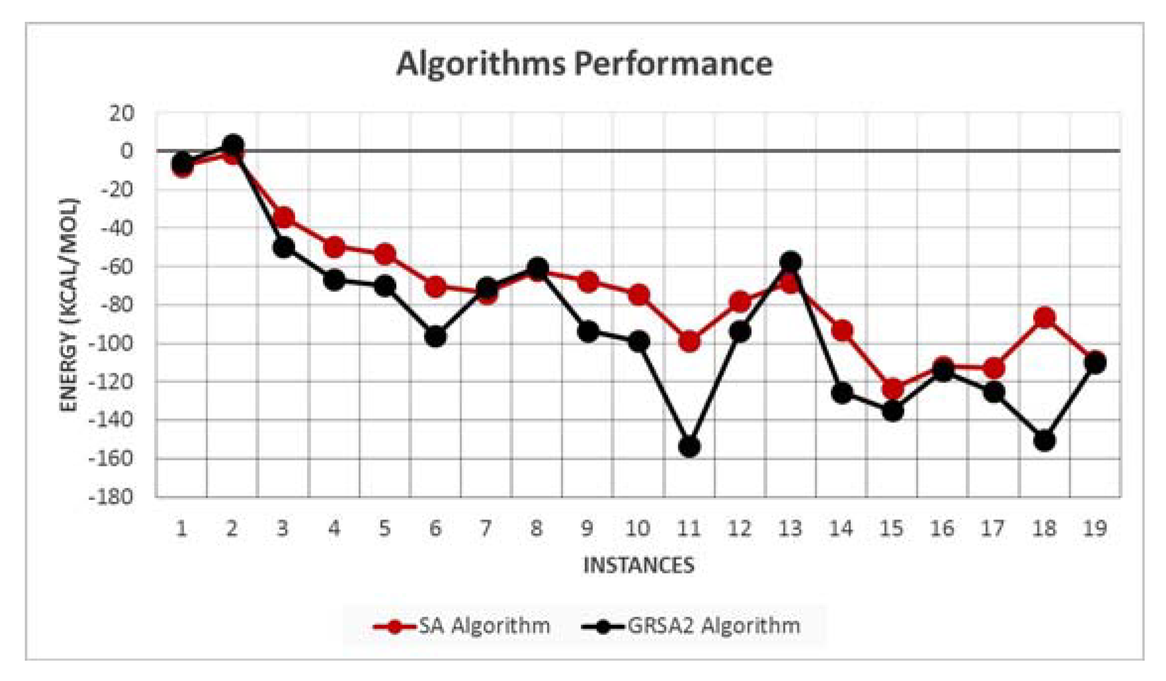
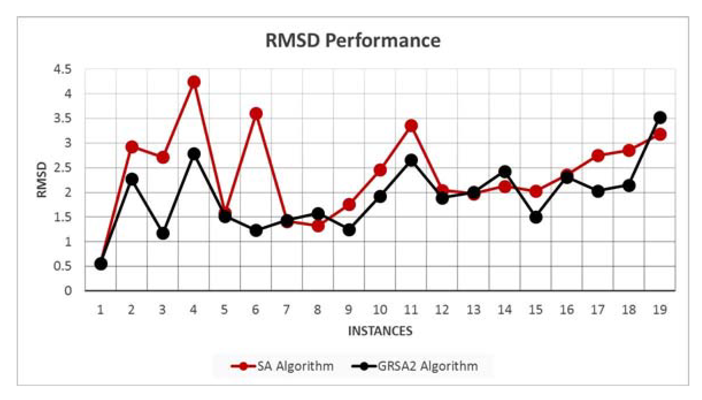
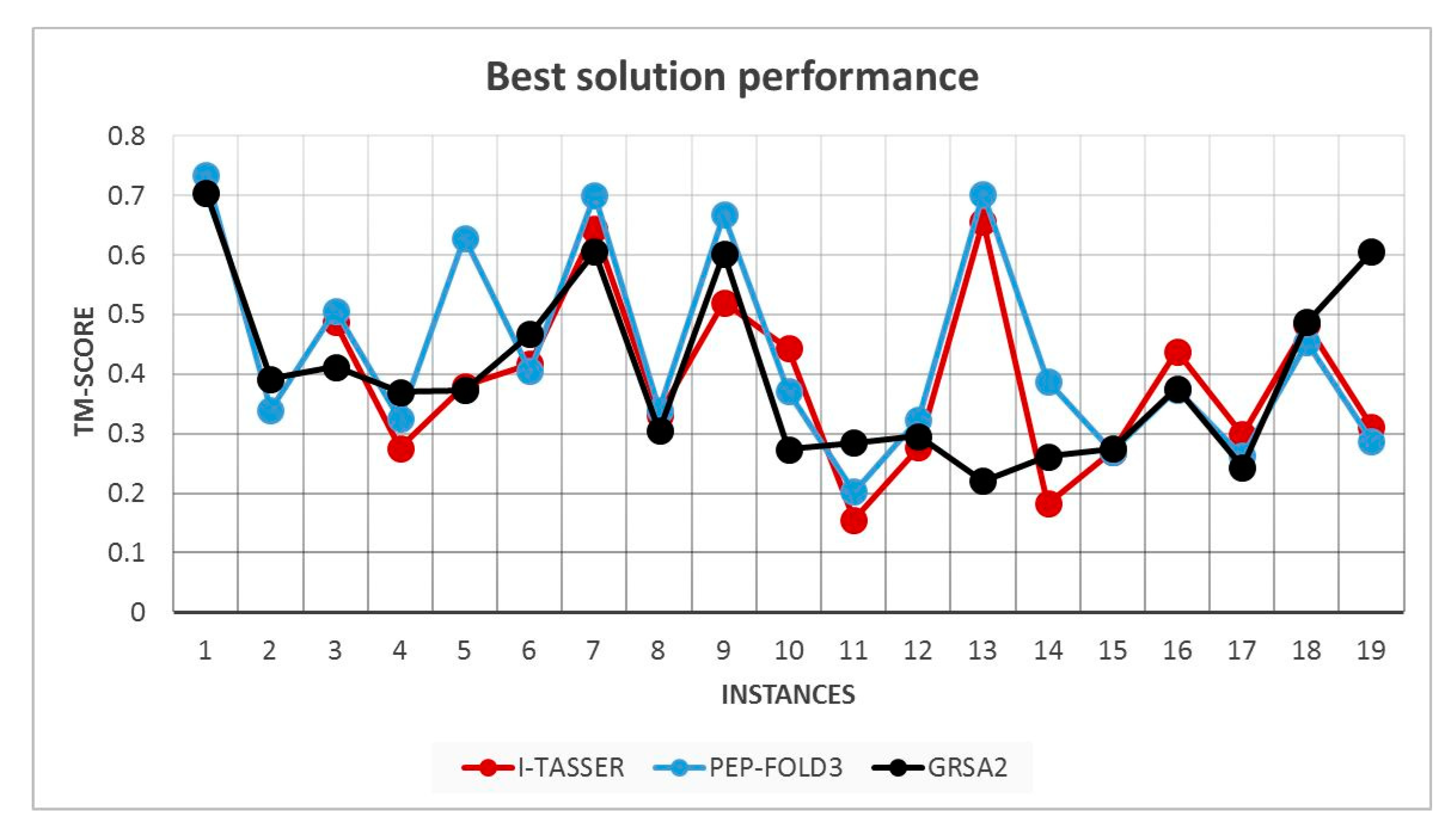
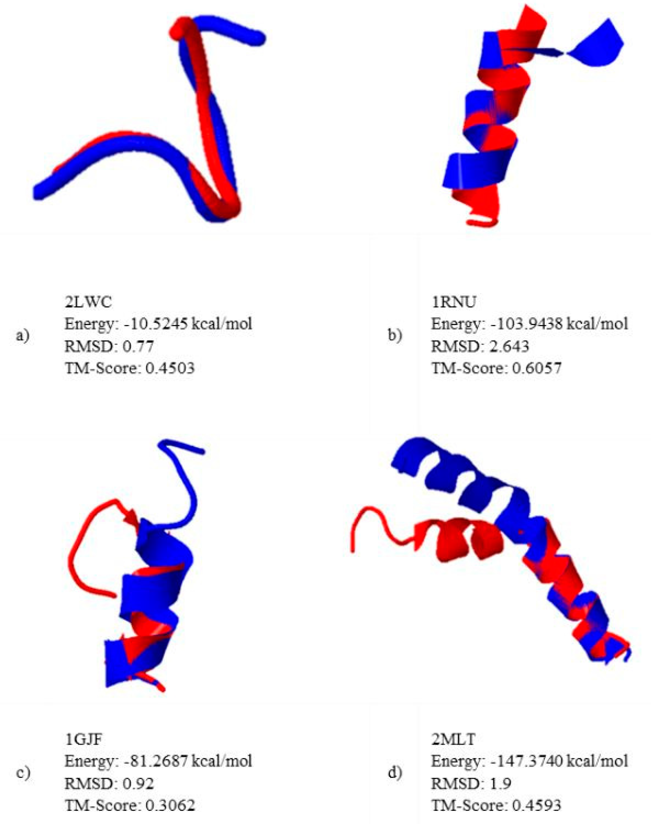
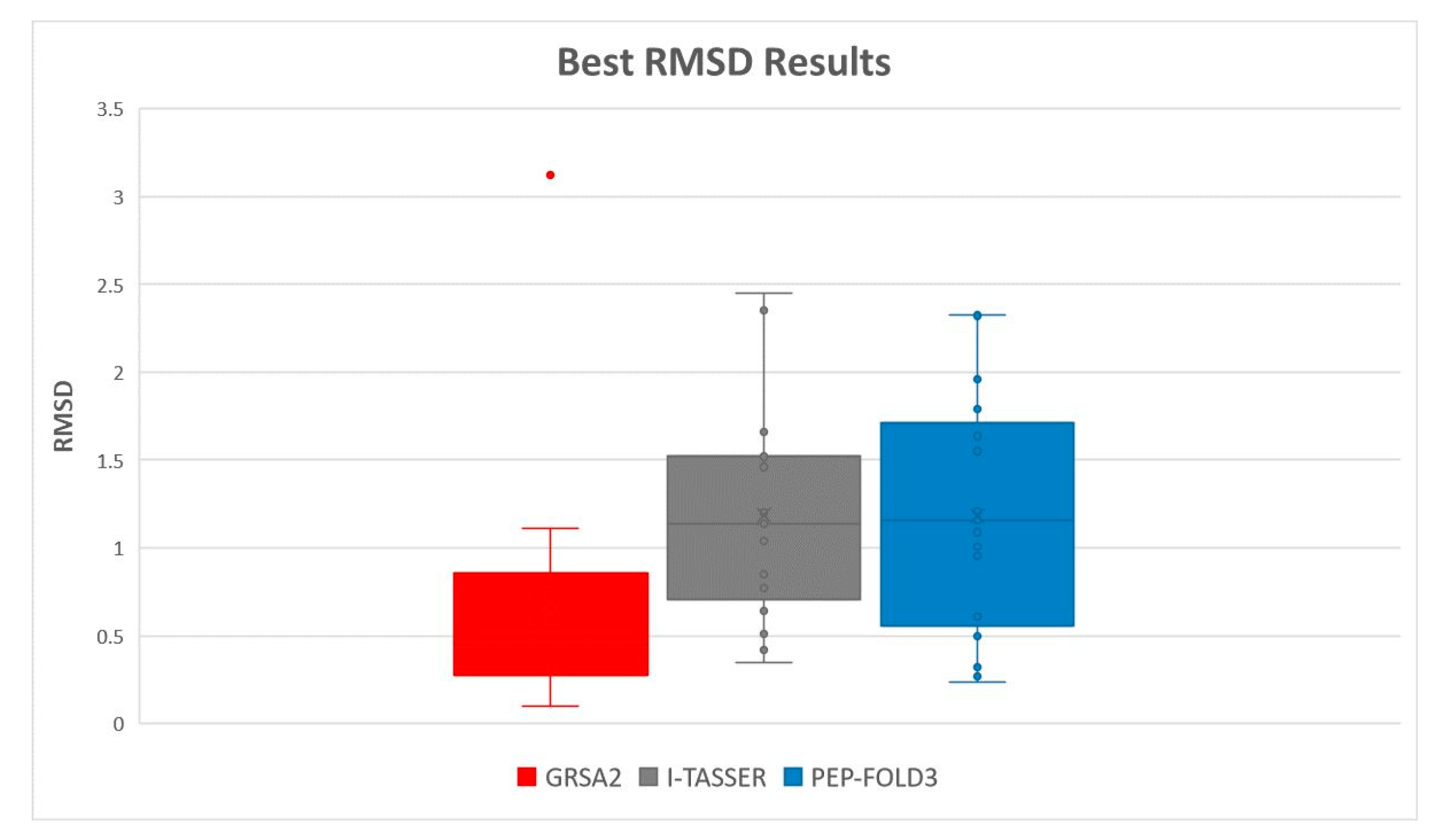
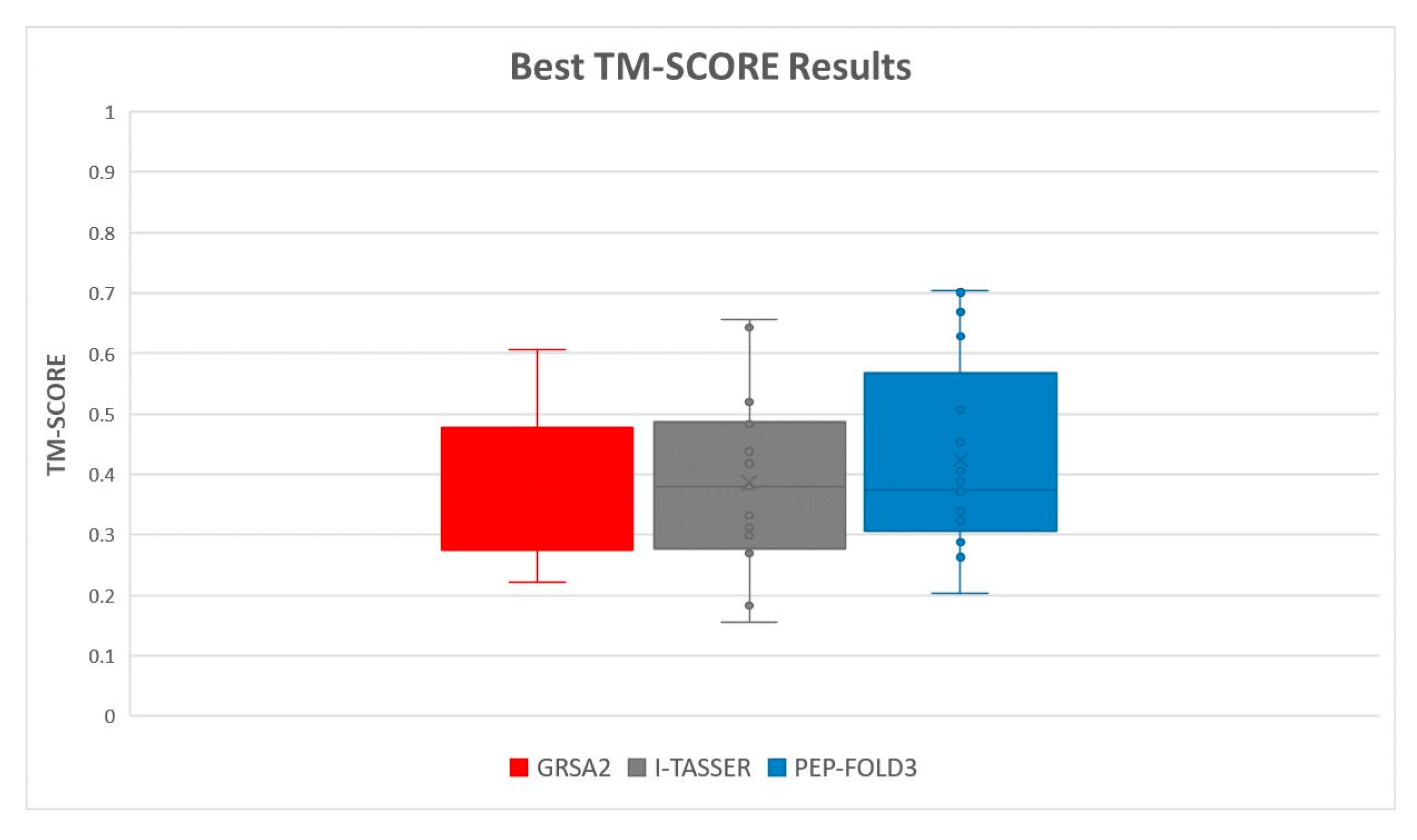
5.2. Results and Discussion
6. Conclusions
Author Contributions
Funding
Acknowledgments
Conflicts of Interest
References
- Khoury, G.A.; Smadbeck, J.; Kieslich, C.A.; Floudas, C.A. Protein Folding and de Novo Protein Design for Biotechnological Applications. Trends Biotechnol. 2014, 32, 99–109. [Google Scholar] [CrossRef] [PubMed]
- Anfinsen, C.B. Principles that Govern the Folding of Protein Chains. Science 1973, 181, 223–230. [Google Scholar] [CrossRef] [PubMed]
- Shin, M.H.; Lim, H.S. Screening Methods for Identifying Pharmacological Chaperones. Mol. Biosyst. 2017, 13, 638–647. [Google Scholar] [CrossRef] [PubMed]
- Hou, Z.S.; Ulloa-Aguirre, A.; Tao, Y.X. Pharmacoperone Drugs: Targeting Misfolded Proteins Causing Lysosomal Storage-, ion Channels-, and G protein-coupled receptors-associated conformational disorders. Expert Rev. Clin. Pharmacol. 2018, 11, 611–624. [Google Scholar] [CrossRef] [PubMed]
- Valastyan, J.S.; Lindquist, S. Mechanisms of Protein-folding Diseases at a Glance. Dis. Model. Mech. 2014, 7, 9–14. [Google Scholar] [CrossRef] [PubMed]
- Sohl, J.L.; Jaswal, S.S.; Agard, D.A. Unfolded Conformations of α-lytic Protease are More Stable Than its Native State. Nature 1998, 395, 817–819. [Google Scholar] [CrossRef]
- Levinthal, C. Are There Pathways for Protein Folding. J. Chim. Phys. 1968, 65, 44–45. [Google Scholar] [CrossRef]
- Yee, A.A.; Savchenko, A.; Ignachenko, A.; Lukin, J.; Xu, X.; Skarina, T.; Edwards, A.M. NMR and X-ray crystallography, complementary tools in structural proteomics of small proteins. J. Am. Chem. Soc. 2005, 127, 16512–16517. [Google Scholar] [CrossRef]
- Hart, W.E.; Istrail, S. Robust Proofs of NP-Hardness for Protein Folding: General Lattices and Energy Potentials. J. Comput. Biol. 1997, 4, 1–22. [Google Scholar] [CrossRef]
- Uhlig, T.; Kyprianou, T.; Martinelli, F.G.; Oppici, C.A.; Heiligers, D.; Hills, D.; Verhaert, P. The Emergence of Peptides in the Pharmaceutical Business: From Exploration to Exploitation. EuPA Open Proteom. 2014, 4, 58–69. [Google Scholar] [CrossRef]
- Fosgerau, K.; Hoffmann, T. Peptide Therapeutics: Current Status and Future Directions. Drug Discov. Today 2015, 20, 122–128. [Google Scholar] [CrossRef] [PubMed]
- Lamiable, A.; Thévenet, P.; Rey, J.; Vavrusa, M.; Derreumaux, P.; Tufféry, P. PEP-FOLD3: Faster de Novo Structure Prediction for Linear Peptides in Solution and in Complex. Nucleic Acids Res. 2016, 44, W449–W454. [Google Scholar] [CrossRef] [PubMed]
- Vetter, I.; Davis, J.L.; Rash, L.D.; Anangi, R.; Mobli, M.; Alewood, P.F.; King, G.F. Venomics: A New Paradigm for Natural Products-based Drug Discovery. Amino Acids 2011, 40, 15–28. [Google Scholar] [CrossRef] [PubMed]
- Frausto-Solis, J.; Sánchez-Hernández, J.P.; Sánchez-Pérez, M.; García, E.L. Golden Ratio Simulated Annealing for Protein Folding Problem. Int. J. Comput. Methods 2015, 12, 1550037. [Google Scholar] [CrossRef]
- Rohl, C.A.; Strauss, C.E.M.; Misura, K.M.S.; Baker, D. Protein Structure Prediction Using Rosetta. In Methods in Enzymology; Elsevier: Amsterdam, The Netherlands, 2004; Volume 383, pp. 66–93. [Google Scholar]
- Xu, D.; Zhang, Y. Ab initio Protein Structure Assembly Using Continuous Structure Fragments and Optimized Knowledge-based Force Field. Proteins Struct. Funct. Bioinform. 2012, 80, 1715–1735. [Google Scholar] [CrossRef] [PubMed]
- Xu, D.; Zhang, Y. Toward Optimal Fragment Generations for ab initio Protein Structure Assembly. Proteins Struct. Funct. Bioinform. 2013, 81, 229–239. [Google Scholar] [CrossRef]
- Yang, J.; Yan, R.; Roy, A.; Xu, D.; Poisson, J.; Zhang, Y. The I-TASSER Suite: Protein Structure and Function Prediction. Nat. Methods 2015, 12, 7–8. [Google Scholar] [CrossRef]
- Kennedy, D.; Norman, C. What Don’t We Know? American Association for the Advancement of Science. Science 2005, 309, 75. [Google Scholar] [CrossRef]
- Dill, K.A.; MacCallum, J.L. The Protein-Folding Problem, 50 Years On. Science 2012, 338, 1042–1046. [Google Scholar] [CrossRef]
- Kaufmann, K.W.; Lemmon, G.H.; DeLuca, S.L.; Sheehan, J.H.; Meiler, J. Practically Useful: What the Rosetta Protein Modeling Suite Can Do for You. Biochemistry 2010, 49, 2987–2998. [Google Scholar] [CrossRef]
- Bienert, S.; Waterhouse, A.; de Beer, T.A.; Tauriello, G.; Studer, G.; Bordoli, L.; Schwede, T. The SWISS-MODEL Repository-new Features and Functionality. Nucleic Acids Res. 2017, 45, D313–D319. [Google Scholar] [CrossRef] [PubMed]
- Nielsen, M.; Lundegaard, C.; Lund, O.; Petersen, T.N. CPHmodels-3.0—Remote Homology Modeling Using Structure-guided Sequence Profiles. Nucleic Acids Res. 2010, 38, W576–W581. [Google Scholar] [CrossRef] [PubMed]
- Kelley, L.A.; Mezulis, S.; Yates, C.M.; Wass, M.N.; Sternberg, M.J.E. The Phyre2 Web Portal for Protein Modeling, Prediction and Analysis. Nat. Protoc. 2015, 10, 845–858. [Google Scholar] [CrossRef] [PubMed]
- Xu, Y.; Xu, D. Protein Threading Using PROSPECT: Design and Evaluation. Proteins Struct. Funct. Genet. 2000, 40, 343–354. [Google Scholar] [CrossRef]
- Soding, J. Protein Homology Detection by HMM-HMM Comparison. Bioinformatics 2005, 21, 951–960. [Google Scholar] [CrossRef]
- Xu, J.; Li, M.; Kim, D.; Xu, Y. RAPTOR: Optimal Protein Threading by Linear Programming. J. Bioinform. Comput. Biol. 2003, 1, 95–117. [Google Scholar] [CrossRef]
- Buchan, D.W.A.; Jones, D.T. EigenTHREADER: Analogous Protein Fold Recognition by Efficient Contact Map Threading. Bioinformatics 2017, 33, 2684–2690. [Google Scholar] [CrossRef]
- Wu, S.; Zhang, Y. LOMETS: A Local Meta-threading-server for Protein Structure Prediction. Nucleic Acids Res. 2007, 35, 3375–3382. [Google Scholar] [CrossRef]
- Wang, Y.; Virtanen, J.; Xue, Z.; Tesmer, J.J.G.; Zhang, Y. Using Iterative Fragment Assembly and Progressive Sequence Truncation to Facilitate Phasing and Crystal Structure Determination of Distantly Related Proteins. Acta Crystallogr. Sect. D Struct. Biol. 2016, 72, 616–628. [Google Scholar] [CrossRef]
- Unger, R.; Moult, J. Finding the Lowest Free Energy Conformation of a Protein is an NP-hard Problem: Proof and Implications. Bull. Math. Biol. 1993, 55, 1183–1198. [Google Scholar] [CrossRef]
- Dorn, M.E.; Silva, M.B.; Buriol, L.S.; Lamb, L.C. Three-dimensional Protein Structure Prediction: Methods and Computational Strategies. Comput. Biol. Chem. 2014, 53, 251–276. [Google Scholar] [CrossRef] [PubMed]
- Delarue, M.; Koehl, P. Combined Approaches from Physics, Statistics, and Computer Science for ab initio Protein Structure Prediction: Ex Unitate Vires (unity is strength)? F1000Research 2018, 7, 1125. [Google Scholar] [CrossRef] [PubMed]
- Melo-Vega, A.; Frausto-Solís, J.; Castilla-Valdez, G.; Liñán-García, E.; González-Barbosa, J.J.; Terán-Villanueva, D. Protein Folding Problem in the Case of Peptides Solved by Hybrid Simulated Annealing Algorithms. In Fuzzy Logic Augmentation of Neural and Optimization Algorithms: Theoretical Aspects and Real Applications; Springer: Cham, Switzerland, 2018; pp. 141–152. [Google Scholar]
- Frausto-Solis, J.; Liñan-García, E.; Sánchez-Pérez, M.; Sánchez-Hernández, J.P. Chaotic Multiquenching Annealing Applied to the Protein Folding Problem. Sci. World J. 2014, 2014, 1–11. [Google Scholar] [CrossRef]
- Li, Z.; Scheraga, H.A. Monte Carlo-minimization Approach to the Multiple-minima Problem in Protein Folding. Proc. Natl. Acad. Sci. USA 1987, 84, 6611–6615. [Google Scholar] [CrossRef] [PubMed]
- Frausto-Solis, J.; Liñán-García, E.; Sánchez-Hernández, J.P.; González-Barbosa, J.J.; González-Flores, C.; Castilla-Valdez, G. Multiphase Simulated Annealing Based on Boltzmann and Bose-Einstein Distribution Applied to Protein Folding Problem. Adv. Bioinform. 2016, 2016, 1–16. [Google Scholar] [CrossRef] [PubMed]
- Vega, A.M.; Frausto-Solís, J.; García, E.L.; Valdez, G.C.; Barbosa, J.J.G.; Villanueva, D.T.; Hernández, J.P.S. Parallel Evolutionary Multi-Quenching Annealing for Protein Folding Problem. Int. J. Comb. Optim. Probl. Inform. 2018, 9, 41–54. [Google Scholar]
- Lam, A.Y.S.; Li, V.O.K. Chemical Reaction Optimization: A tutorial. Memetic Comput. 2012, 4, 3–17. [Google Scholar] [CrossRef]
- Zhang, Y.; Kolinski, A.; Skolnick, J. TOUCHSTONE II: A New Approach to ab initio Protein Structure Prediction. Biophys. J. 2003, 85, 1145–1164. [Google Scholar] [CrossRef]
- Maupetit, J.; Derreumaux, P.; Tuffery, P. PEP-FOLD: An Online Resource for de Novo Peptide Structure Prediction. Nucleic Acids Res. 2009, 37, W498–W503. [Google Scholar] [CrossRef]
- Kryshtafovych, A.; Monastyrskyy, B.; Fidelis, K.; Moult, J.; Schwede, T.; Tramontano, A. Evaluation of the Template-based Modeling in CASP12. Proteins Struct. Funct. Bioinform. 2018, 86, 321–334. [Google Scholar] [CrossRef]
- Kirkpatrick, S.; Gelatt, C.; Vecchi, M. Optimization by Simulated Annealing. Science 1983, 220, 671–680. [Google Scholar] [CrossRef] [PubMed]
- Hansen, P.B. Simulated Annealing. In Electrical Engineering and Computer Science Technical Reports; Syracuse University: Syracuse, NY, USA, 1992; Volume 170. [Google Scholar]
- Alatas, B. ACROA: Artificial Chemical Reaction Optimization Algorithm for Global Optimization. Expert Syst. Appl. 2011, 38, 13170–13180. [Google Scholar] [CrossRef]
- Sanvicente-Sánchez, H.; Frausto-Solís, J. A Method to Establish the Cooling Scheme in Simulated Annealing Like Algorithms. In International Conference on Computational Science and Its Applications; Springer: Berlin/Heidelberg, Germany, 2004; pp. 755–763. [Google Scholar]
- Ponder, J.W.; Case, D.A. Force Fields for Protein Simulations. Adv. Protein Chem. 2003, 66, 27–85. [Google Scholar] [PubMed]
- Brooks, B.R.; Bruccoleri, R.E.; Olafson, B.D.; States, D.J.; Swaminathan, S.; Karplus, M. CHARMM: A Program for Macromolecular Energy, Minimization, and Dynamics Calculations. J. Comput. Chem. 1983, 4, 187–217. [Google Scholar] [CrossRef]
- Eisenmenger, F.; Hansmann, U.H.E.; Hayryan, S.; Hu, C.K. [SMMP] A Modern Package for Simulation of Proteins. Comput. Phys. Commun. 2001, 138, 192–212. [Google Scholar] [CrossRef]
- Meinke, J.H.; Mohanty, S.; Eisenmenger, F.; Hansmann, U.H.E. SMMP v. 3.0-Simulating Proteins and Protein Interactions in Python and Fortran. Comput. Phys. Commun. 2008, 178, 459–470. [Google Scholar] [CrossRef]
- Pronzato, L. A Generalized Golden-section Algorithm for Line Search. IMA J. Math. Control Inf. 1998, 15, 185–214. [Google Scholar] [CrossRef]
- Frausto-Solis, J.; Martinez-Rios, F. Golden Annealing Method for Job Shop Scheduling Problem. In Proceedings of the 10th WSEAS International Conference on Mathematical and Computational Methods in Science and Engineering, Bucharest, Romania, 7–9 November 2008; World Scientific and Engineering Academy and Society (WSEAS): Stevens Point, WI, USA, 2008; pp. 374–379. [Google Scholar]
- Frausto-Solis, J.; Martinez-Rios, F. Golden Ratio Annealing for Satisfiability Problems Using Dynamically Cooling Schemes. In International Symposium on Methodologies for Intelligent Systems; Springer: Berlin/Heidelberg, Germany, 2008; pp. 215–224. [Google Scholar]
- Duek, G.; Scheuer, T. Threshold Accepting: A general Purpose Optimization Algorithm Appearing Superior to Simulated Annealing. J. Comput. Phys. 1990, 90, 161–175. [Google Scholar] [CrossRef]
- Zhan, L.; Chen, J.Z.Y.; Liu, W.K. Conformational Study of Met-Enkephalin Based on the ECEPP Force Fields. Biophys. J. 2006, 91, 2399–2404. [Google Scholar] [CrossRef]
- Zhang, Y.; Skolnick, J. Scoring Function for Automated Assessment of Protein Structure Template Quality. Proteins Struct. Funct. Bioinform. 2004, 57, 702–710. [Google Scholar] [CrossRef]
- Xu, J.; Zhang, Y. How Significant is a Protein Structure Similarity with TM-score = 0.5? Bioinformatics 2010, 26, 889–895. [Google Scholar] [CrossRef] [PubMed]
- Zhang, Y.; Skolnick, J. TM-align: A Protein Structure Alignment Algorithm Based on the TM-score. Nucleic Acids Res. 2005, 33, 2302–2309. [Google Scholar] [CrossRef] [PubMed]
- Wolpert, D.H.; Macready, W.G. No Free Lunch Theorems for Optimization. IEEE Trans. Evol. Comput. 1997, 1, 67–82. [Google Scholar] [CrossRef]
- Papadimitriou, C.H. Computational Complexity; Addison Wesley Longman: Boston, MA, USA, 1994; ISBN 0-201-53082-1. [Google Scholar]


| Number | Instance (PDB Code) | Number of Amino Acids | Number of Variables |
|---|---|---|---|
| 1 | 2LWC | 5 | 19 |
| 2 | 1EGS | 9 | 49 |
| 3 | 1UAO | 10 | 47 |
| 4 | 1L3Q | 12 | 62 |
| 5 | 2EVQ | 12 | 66 |
| 6 | 1IN3 | 12 | 74 |
| 7 | 1RNU | 13 | 68 |
| 8 | 1LCX | 13 | 81 |
| 9 | 1GJF | 14 | 79 |
| 10 | 1K43 | 14 | 84 |
| 11 | 2BTA | 15 | 100 |
| 12 | 1LE3 | 16 | 91 |
| 13 | 1PEF | 18 | 124 |
| 14 | 1L2Y | 20 | 100 |
| 15 | 1DU1 | 210 | 134 |
| 16 | 1PEI | 22 | 143 |
| 17 | 1WZ4 | 23 | 123 |
| 18 | 2MLT | 26 | 158 |
| 19 | 1T0C | 31 | 132 |
| Instances | Average Energy (kcal/mol) | Average RMSD | Average TM-Score |
|---|---|---|---|
| 2LWC | −7.7386 | 0.5538 | 0.5007 |
| 1EGS | −1.0498 | 2.9325 | 0.2816 |
| 1UAO | −34.2519 | 2.7139 | 0.2818 |
| 1L3Q | −49.5822 | 4.2446 | 0.2116 |
| 2EVQ | −53.3023 | 1.5843 | 0.2663 |
| 1IN3 | −70.1176 | 3.6054 | 0.2748 |
| 1RNU | −73.6159 | 1.4122 | 0.3526 |
| 1LCX | −61.9788 | 1.3277 | 0.2436 |
| 1GJF | −67.6448 | 1.76 | 0.2820 |
| 1K43 | −74.1248 | 2.46 | 0.2276 |
| 2BTA | −98.6907 | 3.3561 | 0.1992 |
| 1LE3 | −78.0697 | 2.0468 | 0.1791 |
| 1PEF | −68.1363 | 1.9766 | 0.1780 |
| 1L2Y | −92.8494 | 2.126 | 0.1805 |
| 1DU1 | −123.4410 | 2.0280 | 0.1760 |
| 1PEI | −111.8189 | 2.351 | 0.1435 |
| 1WZ4 | −112.8309 | 2.75 | 0.1572 |
| 2MLT | −86.3540 | 2.8553 | 0.1666 |
| 1T0C | −109.1762 | 3.1829 | 0.1970 |
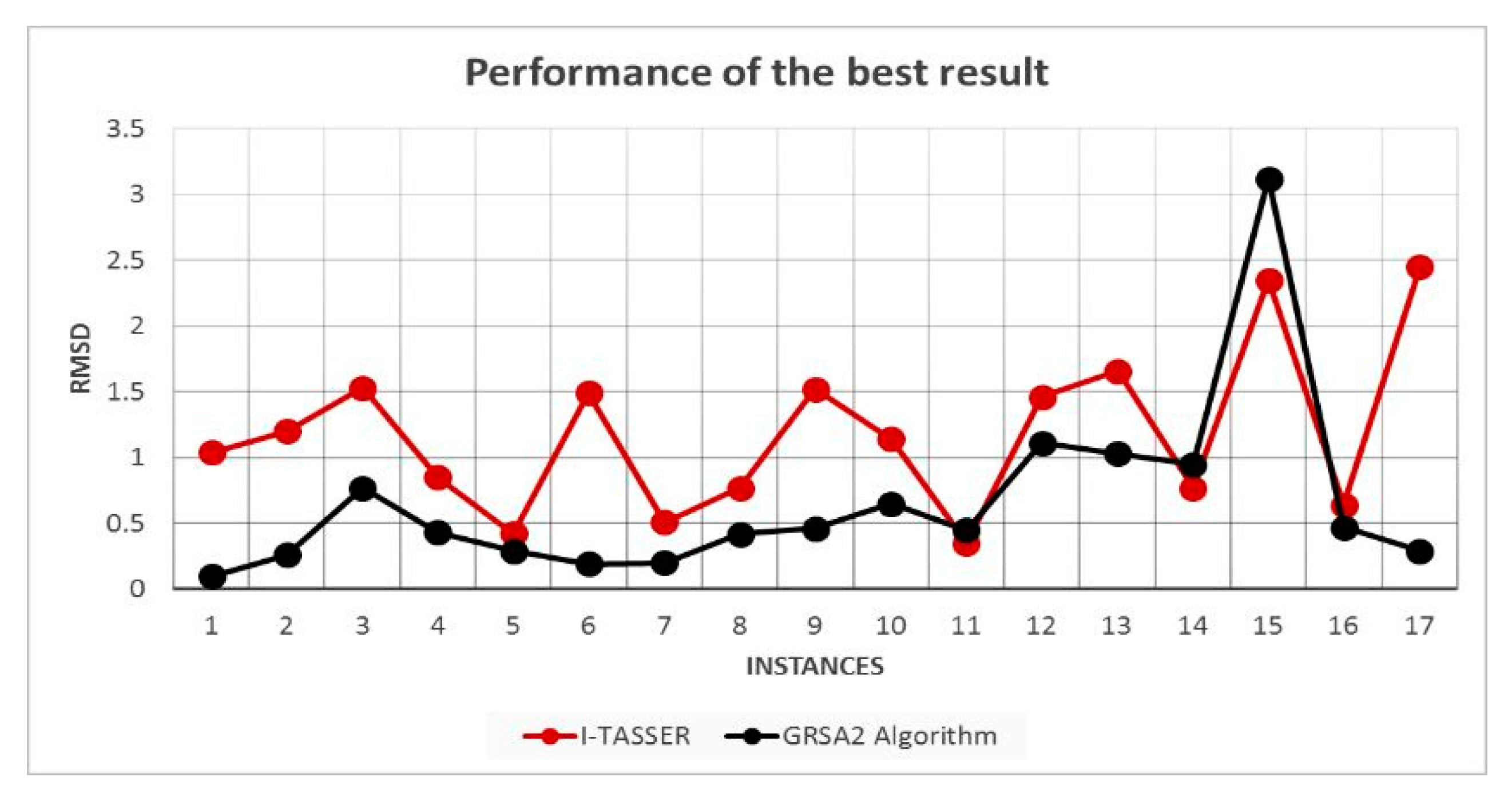
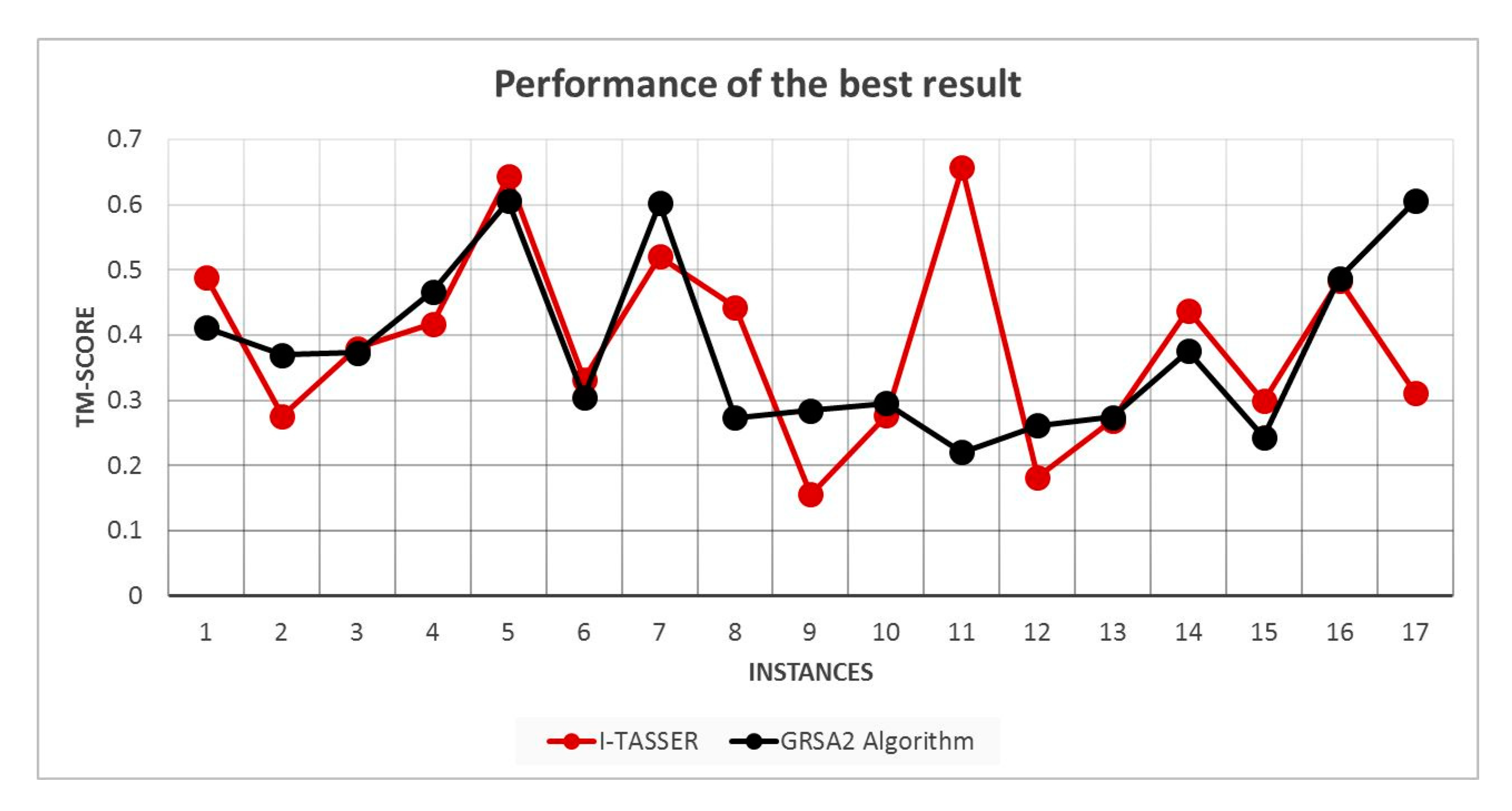
| Instances | Average Energy (kcal/mol) | Average RMSD | Average TM-Score |
|---|---|---|---|
| 2LWC | −5.7567 | 0.5593 | 0.4970 |
| 1EGS | 3.5779 | 2.2703 | 0.2830 |
| 1UAO | −49.4173 | 1.1766 | 0.2718 |
| 1L3Q | −66.6739 | 2.784 | 0.2203 |
| 2EVQ | −69.7577 | 1.5208 | 0.2576 |
| 1IN3 | −96.1027 | 1.2333 | 0.3469 |
| 1RNU | −70.9097 | 1.4382 | 0.2534 |
| 1LCX | −60.4809 | 1.5791 | 0.2205 |
| 1GJF | −93.3798 | 1.2517 | 0.3989 |
| 1K43 | −98.7355 | 1.9287 | 0.1730 |
| 2BTA | −153.3692 | 2.6587 | 0.2075 |
| 1LE3 | −93.4192 | 1.89333 | 0.1773 |
| 1PEF | −57.2994 | 2.0026 | 0.1534 |
| 1L2Y | −125.3933 | 2.4276 | 0.1734 |
| 1DU1 | −134.8380 | 1.5084 | 0.1695 |
| 1PEI | −114.1452 | 2.315 | 0.1936 |
| 1WZ4 | −125.0288 | 2.0323 | 0.1453 |
| 2MLT | −150.0441 | 2.1519 | 0.2899 |
| 1T0C | −110.1145 | 3.5264 | 0.1999 |
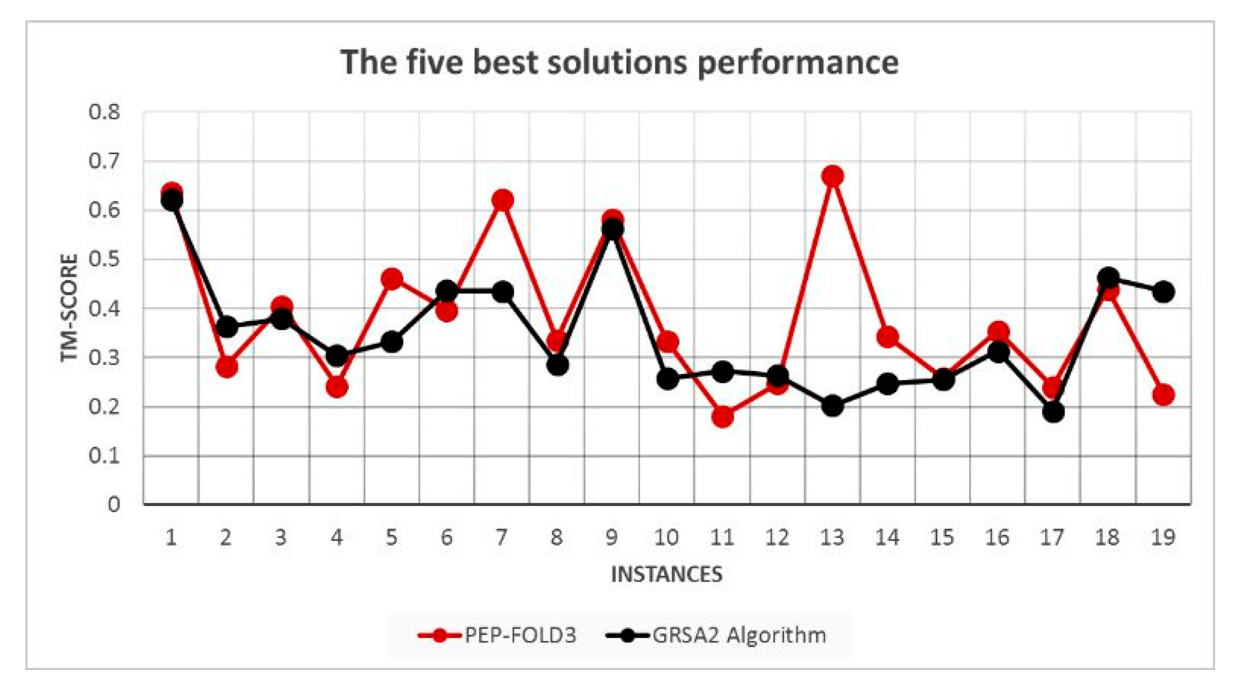
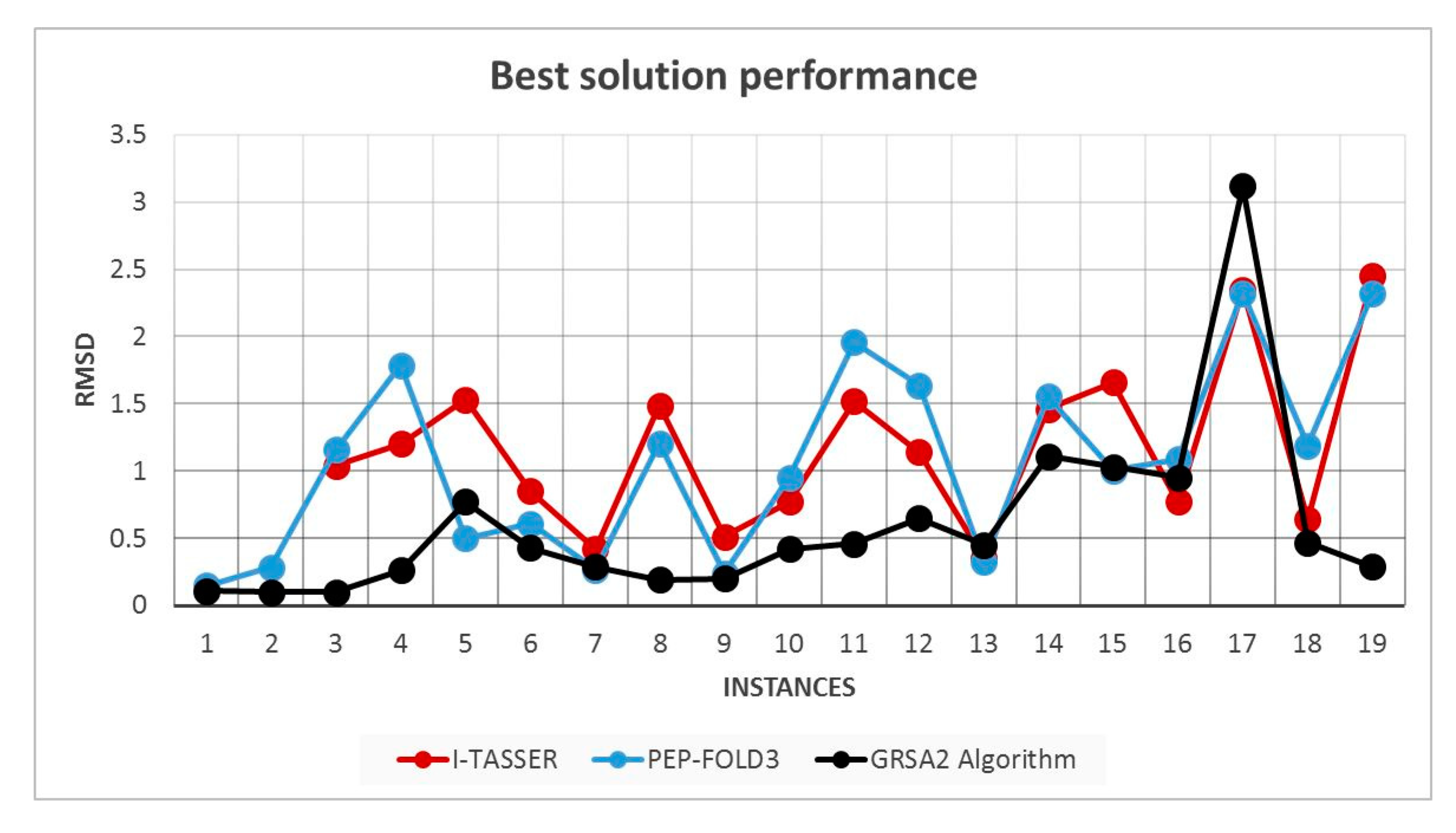
| Instances | RMSD GRSA2 | RMSD PEP-FOLD3 | TM-Score GRSA2 | TM-Score PEP-FOLD3 |
|---|---|---|---|---|
| 2LWC | 0.134 | 0.49915802 | 0.622022 | 0.63645887 |
| 1EGS | 0.174 | 0.73379194 | 0.363588 | 0.28297143 |
| 1UAO | 0.218 | 1.43239212 | 0.379374 | 0.40506025 |
| 1L3Q | 0.49 | 2.11590502 | 0.304162 | 0.24278709 |
| 2EVQ | 0.842 | 0.82452263 | 0.332682 | 0.46217599 |
| 1IN3 | 0.604 | 0.92708461 | 0.436492 | 0.39695857 |
| 1RNU | 0.352 | 0.80774343 | 0.435094 | 0.62276608 |
| 1LCX | 0.552 | 1.22937939 | 0.287596 | 0.33622833 |
| 1GJF | 0.308 | 0.65046896 | 0.562328 | 0.58219463 |
| 1K43 | 0.782 | 1.50581118 | 0.258046 | 0.33411994 |
| 2BTA | 0.594 | 2.43201208 | 0.27246 | 0.18155674 |
| 1LE3 | 0.826 | 1.96238744 | 0.263946 | 0.24700389 |
| 1PEF | 0.712 | 0.61298789 | 0.20271 | 0.66990523 |
| 1L2Y | 1.312 | 1.86484044 | 0.247734 | 0.3428772 |
| 1DU1 | 1.286 | 1.29916825 | 0.256142 | 0.25837997 |
| 1PEI | 1.198 | 1.29391279 | 0.313088 | 0.35394815 |
| 1WZ4 | 3.034 | 2.74149027 | 0.191944 | 0.23998161 |
| 2MLT | 0.972 | 1.57230256 | 0.462832 | 0.43948739 |
| 1T0C | 0.352 | 3.21218634 | 0.435094 | 0.22636347 |
© 2019 by the authors. Licensee MDPI, Basel, Switzerland. This article is an open access article distributed under the terms and conditions of the Creative Commons Attribution (CC BY) license (http://creativecommons.org/licenses/by/4.0/).
Share and Cite
Frausto-Solís, J.; Sánchez-Hernández, J.P.; Maldonado-Nava, F.G.; González-Barbosa, J.J. GRSA Enhanced for Protein Folding Problem in the Case of Peptides. Axioms 2019, 8, 136. https://doi.org/10.3390/axioms8040136
Frausto-Solís J, Sánchez-Hernández JP, Maldonado-Nava FG, González-Barbosa JJ. GRSA Enhanced for Protein Folding Problem in the Case of Peptides. Axioms. 2019; 8(4):136. https://doi.org/10.3390/axioms8040136
Chicago/Turabian StyleFrausto-Solís, Juan, Juan Paulo Sánchez-Hernández, Fanny G. Maldonado-Nava, and Juan J. González-Barbosa. 2019. "GRSA Enhanced for Protein Folding Problem in the Case of Peptides" Axioms 8, no. 4: 136. https://doi.org/10.3390/axioms8040136
APA StyleFrausto-Solís, J., Sánchez-Hernández, J. P., Maldonado-Nava, F. G., & González-Barbosa, J. J. (2019). GRSA Enhanced for Protein Folding Problem in the Case of Peptides. Axioms, 8(4), 136. https://doi.org/10.3390/axioms8040136