Deduction in Non-Fregean Propositional Logic SCI

Abstract

We study deduction systems for the weakest, extensional and two-valued non-Fregean propositional logic $\mathsf{SCI}$. The language of $\mathsf{SCI}$ is obtained by expanding the language of classical propositional logic with a new binary connective ≡ that expresses the identity of two statements; that is, it connects two statements and forms a new one, which is true whenever the semantic correlates of the arguments are the same. On the formal side, $\mathsf{SCI}$ is an extension of classical propositional logic with axioms characterizing the identity connective, postulating that identity must be an equivalence and obey an extensionality principle. First, we present and discuss two types of systems for $\mathsf{SCI}$ known from the literature, namely sequent calculus and a dual tableau-like system. Then, we present a new dual tableau system for $\mathsf{SCI}$ and prove its soundness and completeness. Finally, we discuss and compare the systems presented in the paper.

1. Introduction

One of the tasks of formal logic is to provide adequate tools for the formal analysis of certain fragments of natural language, as well as for the languages of particular fields of science. It is commonly accepted that the theory of interpretation of a language is semantics. The choice of semantics determines how we think about a given language and what meaning we assign to its components. It is often acknowledged that the first precisely formulated semantic principles—that serves as a foundation for contemporary formal logic and have determined its development—were presented by Frege in his Begriffsschrift. According to Frege, a correct and adequate formal system of a given language should meet the following conditions:

F1 

All names and all sentences have meaning and denotation. Meaning is not the same as denotation.

F2 

A name and a sentence are the proper names of their denotations.

F3 

Only one logical value can be assigned to each sentence: true or false.

F4 

If two expressions have the same denotation, then they are exchangeable in any propositional context of a sentence without changing the logical value of that sentence.

F5 

If two sentences are exchangeable in any propositional context of a sentence without changing its logical value, then they have the same denotation.

Note that crucial notions for Frege’s account are the following: meaning, denotation, and logical valuation. Frege admits that the meaning of a sentence is not the same as its denotation. Indeed, the same holds for names: ‘Evening Star’ and ‘Morning Star’ denote the same object, but they have different meanings. The meaning of a sentence should be understood as its sense that the sentence expresses. Thus, we should ask what a sentence is referring to. From the formal point of view, the answer to this question requires, in particular, to decide what the denotation of a propositional variable is.

Propositional variables have an unusual character due to the fact that, at the same time, they are formulas. In classical logic, this ambiguity is removed as it identifies denotations of sentences with their truth values. In other words, in classical logic, propositional variables occur only at the metalogical level (they are not treated as real variables) or, as it holds in propositional calculus, variables range over the two element set of logical values. Within such an account, only terms have a meaningful ontological reference. Thus, the advocate of classical logic, if he is also a proponent of the Fregean semantic principles, must accept that all true sentences have one and the same denotation, namely the logical value $\mathsf{Truth}$, and denotation of all false sentences is the logical value $\mathsf{False}$.

The consequence of Frege’s semantic principles, according to which denotations of sentences are logical values, is usually called the Fregean principle, and every logical system that adopts this principle is called a Fregean system. The Fregean approach can be considered as philosophically justified in the study of mathematical languages, but it is not obvious that such an approach is justified as a foundation of a philosophically adequate semantics. The debatable cases of the applicability of the Fregean account in the formalization of any language are, for instance, theories of meaning or ontology. If we admit that the references of sentences are situations (states of affairs) that these sentences describe (in analogy with the assumption that the semantic references of terms are objects named by these terms), then the Fregean principle is not only a semantic principle, but also an ontological one which imposes a quantitative restriction on the universe of situations: there are at most two situations described by sentences. This is an extremely strong assumption. Note that the Fregean account does not impose an upper limit on the universe of objects.

Roman Suszko in 1968 [1] proposed to change the Fregean paradigm and introduced the so-called non-Fregean logic (see also [2]). The basic philosophical assumption underlying non-Fregean logic is the thesis in reality to which the language is referring, and there exist semantic correlates of all expressions that are not purely syntactic. Therefore, in the non-Fregean approach, it is assumed that the semantic correlates of names are objects from the universe of objects, the semantic correlates of predicates are appropriate sets, and the semantic correlates of sentences are situations described by these sentences. Furthermore, a universe of situations cannot be quantitatively restricted, except that there are at least two situations.

The construction of a propositional non-Fregean logic, which at the same time preserves all properties of classical logic with respect to the classical connectives, is relatively simple. To make it possible to express statements on situations and interactions between them, propositional calculus is extended with the additional connective, named the identity connective and denoted by ≡. The intended interpretation of the identity connective is the following: $\varphi \equiv \psi$ is true if and only if the semantic correlates of $\varphi$ and $\psi$ are the same, that is, sentences $\phi$ and $\psi$ describe the same situation (the same state of affairs). Note that, in a general case, the identity connective is different than the classical equivalence. Equivalent sentences, that is, sentences that do not have the same logical value, do not have to refer to the same situation, and so they do not have to be identical. In other words, the logical value of a sentence and the situation described by this sentence are two different things.

Suszko states that the identity connective is more primitive than other non-truth functional connectives such as modal connectives of possibility and necessity. The identity connective is more primitive in the sense that it cannot be eliminated without identifying it with the equivalence connective. However, if we add the identity connective to classical logic, we do not lose two-valuedness. If a non-Fregean system of logic would be constructed based on classical logic, extending its language with the identity connective and constructing semantics in which classical connectives preserve their classical meaning, we will obtain a two-valued system, in which each sentence is either true or false. On the other hand, being logically two-valued, non-Fregean logics can be seen as systems that are ontologically (referentially) many-valued.

The weakest extensional and two-valued propositional non-Fregean logic is $\mathsf{SCI}$ (Sentential Calculus with Identity). A detailed description of the philosophical assumptions of $\mathsf{SCI}$ can be found in [2]. Originally, logic $\mathsf{SCI}$ was defined as an extension of classical propositional logic with four axioms expressing the following properties of the identity connective: (1) any sentence is identical with itself, (2) if two sentences are identical, then so are their negations, (3) identical sentences are equivalent, and (4) sentences that are identical are interchangeable in any propositional context. A sound and complete semantics for $\mathsf{SCI}$ was designed by Suszko and Bloom in [3]. A models for $\mathsf{SCI}$ is a structure that consists of a universe of situations, a distinguished subset of facts (situations that actually hold), and operations that represent all the connectives. Furthermore, it is assumed that the operations satisfy certain conditions with respect to the distinguished set of situations so that the classical connectives gain their classical meaning, and the operation corresponding to the identity connective represents the identity between situations. For details, see Section 2.

It is established that $\mathsf{SCI}$ has the finite model property and is decidable. Moreover, as shown in [4], the class of different axiomatic extensions of $\mathsf{SCI}$ is uncountable. There is also some research on non-standard (deviant) modifications of $\mathsf{SCI}$ obtained by rejecting some of its fundamental assumptions or extending its language with additional operators. Recently, the most studied modifications of $\mathsf{SCI}$ are Grzegorczyk’s non-Fregean logics, which are paraconsistent non-Fregean logics ([5,6,7]). Some research has been also focused on first-order non-Fregean logics, in particular ${\mathsf{SCI}}_{\mathsf{Q}}$. In [8], it has been proved that the logic ${\mathsf{SCI}}_{\mathsf{Q}}$, obtained by extending $\mathsf{SCI}$ with propositional quantifiers, is able to express infiniteness and many well-known mathematical theories (e.g., the theories of groups and fields, Peano arithmetic). Furthermore, ${\mathsf{SCI}}_{\mathsf{Q}}$ does not have the finite model property, is undecidable, satisfies the Löwenheim-Skolem Theorem, and is an analog of Fagin’s Theorem (the class of sets of natural numbers that are expressible in ${\mathsf{SCI}}_{\mathsf{Q}}$ is precisely the complexity class $\mathsf{NP}$).

The non-Fregean approach has many philosophical and logical advantages as it offers a relatively simple, natural and intuitive basis for exploring fundamental relationships between language and situations. Moreover, non-Fregean logics can be seen as a general framework for representing and comparing logics with different languages or semantics. Indeed, it turned out that many non-classical logics can be equivalently translated into some extensions of $\mathsf{SCI}$. For instance, modal logics $\mathsf{S}3$, $\mathsf{S}\mathsf{4}$, and $\mathsf{S}\mathsf{5}$ are equivalent to some extensions of $\mathsf{SCI}$, that is, there are translations—from a non-Fregean language to a modal one and the other way round—that preserve the satisfaction of formulas with respect to the appropriate class of structures (see [9]). It has been also proved in [10] that $\mathsf{SCI}$ can serve as a basis for expressing many-valued logics. Furthermore, it has been shown that the weakest non-Fregean logic $\mathsf{MGL}$ (Minimal Grzegorczyk Logic) introduced in [11] is able to express most non-classical logics, including uncountably many extensions of $\mathsf{SCI}$ and paraconsistent non-Fregean Grzegorczyk’s logics. Thus, $\mathsf{MGL}$ can be treated as a generic non-Fregean logic.

The non-Fregean approach could be relevant in cognitive science applications as well as in natural language processing. Last but not least, research on non-Fregean logics could lead to a better understanding of the capabilities and relationships of logics with mutually incompatible languages and semantics. Studies on various versions of non-Fregean logic may also shed light on which class of logics offers the most adequate account of logical symbols from point of view of natural language.

In this paper, we focus on deduction systems for the logic $\mathsf{SCI}$. The deduction system for $\mathsf{SCI}$ was originally defined in a Hilbert-style. Since then, some other systems for $\mathsf{SCI}$ have been proposed: Gentzen sequent calculus ([12,13,14]) and a dual tableau system ([15,16]). The aim of the paper is to present a new dual tableau system for $\mathsf{SCI}$, which is suitable for automated reasoning in $\mathsf{SCI}$. The main advantage of the new system is that, contrary to previously known systems, it is more efficient: it does not involve any substitution rule, its rules for the identity connective do not branch a proof tree, and it generates shorter and simpler proof trees.

The paper consists of five sections: in Section 2, we present the basics of the non-Fregean propositional logic $\mathsf{SCI}$, that is, its language, semantics, and axiomatization. In Section 3 and Section 4, we briefly survey sequent calculus and a dual tableau system for $\mathsf{SCI}$, respectively. In Section 5, we present a new dual tableau system for $\mathsf{SCI}$ and prove its soundness and completeness. Finally, in Section 6, we discuss and compare the systems presented in the paper.

2. The Non-Fregean Propositional Logic $\mathsf{SCI}$

The vocabulary of the language of the non-fregean propositional logic, $\mathsf{SCI}$, consists of the symbols from the following pairwise disjoint sets:

• $\mathbb{V}=\{p_1,p_2,p_3,\dots \}$—a countable infinite set of propositional variables;
• $\{\neg ,\vee ,\wedge ,\to ,\leftrightarrow ,\equiv \}$—the set of propositional operations of negation ¬, disjunction ∨, conjunction ∧, implication →, equivalence ↔, and identity ≡.

The set $\mathbb{FOR}$ of all $\mathsf{SCI}$-formulas is the smallest set including $\mathbb{V}$ and closed with respect to all propositional operations.

An $\mathsf{SCI}$-model is a structure $\mathcal{M}=(U,\sim ,\bigsqcup ,\sqcap ,\Rightarrow ,\iff ,\circ ,D)$, where U is a non-empty set referred to as a universe, D is any non-empty proper subset of U, and $\sim ,\bigsqcup ,\sqcap ,\Rightarrow ,\iff ,\circ$ are operations on U with arities 1, 2, 2, 2, 2, 2, respectively, such that, for all $a,b\in U$ the following hold:

• (SCI1) $\sim a\in D \mathrm{iff} (a\notin D)$;
• (SCI2) $a\bigsqcup b\in D \mathrm{iff} (a\in D \mathrm{or} b\in D)$;
• (SCI3) $a\sqcap b\in D \mathrm{iff} (a\in D \mathrm{and} b\in D)$;
• (SCI4) $a\Rightarrow b\in D \mathrm{iff} (a\notin D \mathrm{or} b\in D)$;
• (SCI5) $a\iff b\in D \mathrm{iff} (a\in D \mathrm{if} \mathrm{and} \mathrm{only} \mathrm{if} b\in D)$;
• (SCI6) $a\circ b\in D \mathrm{iff} a=b$.

Let $\mathcal{M}$ be an $\mathsf{SCI}$-model. A valuation in $\mathcal{M}$ is any mapping $v:\mathbb{FOR}\to U$ such that $v\left(p\right)\in D$, for every $p\in \mathbb{V}$, and the following conditions hold for all $\mathsf{SCI}$-formulas:

$v(\neg \phi )=\sim v\left(\phi \right)$	$v(\phi \to \psi )=v\left(\phi \right)\Rightarrow v\left(\psi \right)$
$v(\phi \vee \psi )=v\left(\phi \right)\bigsqcup v\left(\psi \right)$	$v(\phi \wedge \psi )=v\left(\phi \right)\sqcap v\left(\psi \right)$
$v(\phi \leftrightarrow \psi )=v\left(\phi \right)\iff v\left(\psi \right)$	$v(\phi \equiv \psi )=v\left(\phi \right)\circ v\left(\psi \right)$

Given an $\mathsf{SCI}$-model $\mathcal{M}$ and a valuation v in $\mathcal{M}$, an $\mathsf{SCI}$-formula $\phi$ is said to be satisfied in $\mathcal{M}$ by v (in short $\mathcal{M},v\models \phi$) whenever $v\left(\phi \right)\in D$. An $\mathsf{SCI}$-formula $\phi$ is true in $\mathcal{M}$ if and only if for every v in $\mathcal{M}$, $\mathcal{M},v\models \phi$. A formula is $\mathsf{SCI}$-valid if and only if it is true in all $\mathsf{SCI}$-models. An $\mathsf{SCI}$-formula $\phi$ is said to be satisfiable in an $\mathsf{SCI}$-model $\mathcal{M}$ whenever there exists a valuation v on $\mathcal{M}$ such that $\mathcal{M},v\models \phi$. A model is referred to as finite if its universe is finite.

The intended philosophical interpretation of an $\mathsf{SCI}$-model $\mathcal{M}=(U,\sim ,\bigsqcup ,\sqcap ,\Rightarrow ,\iff ,\circ ,D)$ is as follows: U is the set of situations (denotations of sentences); D is the set of facts, that is, it consists of those situations that correspond to true sentences; the operations correspond to the formation of new formulas with connectives.

The logic $\mathsf{SCI}$ is two-valued. We may define the logical value of a formula $\phi$ in a model $\mathcal{M}$ as:

$$va{l}_{\mathcal{M}}\left(\phi \right)\stackrel{\mathrm{df}}{=}\left\{\begin{array}{cc}\mathrm{t}\mathrm{r}\mathrm{u}\mathrm{e},\hfill & \mathrm{i}\mathrm{f} \mathrm{f}\mathrm{o}\mathrm{r} \mathrm{e}\mathrm{v}\mathrm{e}\mathrm{r}\mathrm{y} v \mathrm{i}\mathrm{n} \mathcal{M},v\left(\phi \right)\in D,\hfill \\ \mathrm{f}\mathrm{a}\mathrm{l}\mathrm{s}\mathrm{e},\hfill & \mathrm{o}\mathrm{t}\mathrm{h}\mathrm{e}\mathrm{r}\mathrm{w}\mathrm{i}\mathrm{s}\mathrm{e}.\hfill \end{array}\right.$$

The following proposition shows that $\mathsf{SCI}$ is extensional in the sense that any subformula $\psi$ of an $\mathsf{SCI}$-formula $\phi$ can be replaced with another formula $\vartheta$ denoting the same as $\psi$ without affecting the denotation of $\phi$.

Proposition 1.

Let $\mathcal{M}$ be an $\mathsf{SCI}$-model, let v be a valuation in $\mathcal{M}$, let φ be an $\mathsf{SCI}$-formula containing a subformula ψ, and let ${\phi }^{\prime }$ be the result of replacing some occurrences of ψ in φ by a formula ϑ. Then, $\mathcal{M},v\models \psi \equiv \vartheta$ implies $\mathcal{M},v\models \phi \equiv {\phi }^{\prime }$.

The proof of Proposition 1 is presented in [16]. It should be emphasized that two-valuedness and extensionality concern different levels. Two-valuedness is a property of truth values, while extensionality holds for denotations.

As shown in [3], the logic $\mathsf{SCI}$ has the finite model property and is decidable:

Theorem 1

(Finite model property and decidability of $\mathsf{SCI}$). The logic $\mathsf{SCI}$ has the finite model property, i.e., every satisfiable $\mathsf{SCI}$-formula is satisfiable in a finite $\mathsf{SCI}$-model. Furthermore, the logic $\mathsf{SCI}$ is decidable.

Corollary 1.

Let T be a set of $\mathsf{SCI}$-formulas such that T is true in all finite $\mathsf{SCI}$-models. Then, T is true in all infinite $\mathsf{SCI}$-models as well.

The proof of the above corollary can be found in [8].

A Hilbert-style axiomatization of $\mathsf{SCI}$ consists of axiom schemas of classical propositional logic $\mathsf{PC}$, which characterize the operations $\neg ,\vee ,\wedge ,\to ,\leftrightarrow$, and the following axiom schemas for the identity operation ≡:

• (${\equiv }_1$)$\phi \equiv \phi$;
• (${\equiv }_2$) $(\phi \equiv \psi )\to (\neg \phi \equiv \neg \psi )$;
• (${\equiv }_3$) $(\phi \equiv \psi )\to (\phi \to \psi )$;
• (${\equiv }_4$) $\left[\right(\phi \equiv \psi )\wedge (\vartheta \equiv \xi \left)\right]\to \left[\right(\phi \#\vartheta )\equiv (\psi \#\xi \left)\right]$, for $\#\in \{\wedge ,\vee ,\to ,\leftrightarrow ,\equiv \}$.

The only rule of inference is modus ponens. The notion of provability of a formula is defined as usual. Thus, an $\mathsf{SCI}$-formula $\phi$ is said to be $\mathsf{SCI}$-provable whenever there exists a finite sequence ${\phi }_1,\dots ,{\phi }_n$ of $\mathsf{SCI}$-formulas, $n\ge 1$, such that ${\phi }_n=\phi$ and each ${\phi }_i$, $i\in \{1,\dots ,n\}$, is an $\mathsf{SCI}$-axiom or follows from earlier formulas in the sequence by the modus ponens rule. It is easy to see that all theorems of classical propositional logic are $\mathsf{SCI}$-provable formulas.

Fact 2.

For every $\mathsf{PC}$-formula φ, the following conditions are equivalent:

1.

φ is provable in the classical propositional logic.

2.

φ is $\mathsf{SCI}$-provable.

Soundness and completeness of $\mathsf{SCI}$ with respect to the class of $\mathsf{SCI}$-models was proved in [3].

Theorem 2

(Soundness and Completeness of $\mathsf{SCI}$). For every $\mathsf{SCI}$-formula φ, the following conditions are equivalent:

1.

φ is $\mathsf{SCI}$-provable.

2.

φ is $\mathsf{SCI}$-valid.

The logic $\mathsf{SCI}$ is very weak as it does not impose any specific assumptions on the cardinality of the universe of situations (except that it has at least two elements). Furthermore, it does not assume any specific assumptions on the identities of equivalent formulas—for instance, the formula $(\phi \wedge \psi )\equiv (\psi \wedge \phi )$ is not $\mathsf{SCI}$-valid. Indeed, the reduct $(U,\sim ,\bigsqcup ,\sqcap )$ of an $\mathsf{SCI}$-model is not necessarily a Boolean algebra, since, for example, $a\sqcap b=b\sqcap a$ is not true in all $\mathsf{SCI}$-models. Consider an $\mathsf{SCI}$-model $\mathcal{M}=(U,\sim ,\bigsqcup ,\sqcap ,\Rightarrow ,\iff ,\circ ,D)$, where $U=\{0,1,2\}$, $D=\{1,2\}$, and the operations $\sim ,\bigsqcup ,\sqcap ,\Rightarrow ,\iff ,\circ$ are defined by:

$\sim a\stackrel{\mathrm{df}}{=}\left\{\begin{array}{cc}0,\hfill & \mathrm{i}\mathrm{f} a\ne 0,\hfill \\ 1,\hfill & \mathrm{o}\mathrm{t}\mathrm{h}\mathrm{e}\mathrm{r}\mathrm{w}\mathrm{i}\mathrm{s}\mathrm{e},\hfill \end{array}\right.$	$a\bigsqcup b\stackrel{\mathrm{df}}{=}\left\{\begin{array}{cc}0,\hfill & \mathrm{i}\mathrm{f} a=0 \mathrm{a}\mathrm{n}\mathrm{d} b=0,\hfill \\ 1,\hfill & \mathrm{o}\mathrm{t}\mathrm{h}\mathrm{e}\mathrm{r}\mathrm{w}\mathrm{i}\mathrm{s}\mathrm{e},\hfill \end{array}\right.$
$a\Rightarrow b\stackrel{\mathrm{df}}{=}\left\{\begin{array}{cc}0,\hfill & \mathrm{i}\mathrm{f} a\ne 0 \mathrm{a}\mathrm{n}\mathrm{d} b=0,\hfill \\ 1,\hfill & \mathrm{o}\mathrm{t}\mathrm{h}\mathrm{e}\mathrm{r}\mathrm{w}\mathrm{i}\mathrm{s}\mathrm{e},\hfill \end{array}\right.$	$a\sqcap b\stackrel{\mathrm{df}}{=}\left\{\begin{array}{cc}0,\hfill & \mathrm{i}\mathrm{f} a=0, \mathrm{o}\mathrm{r} b=0,\hfill \\ 1,\hfill & \mathrm{i}\mathrm{f} b=2 \mathrm{a}\mathrm{n}\mathrm{d} a\ne 0,\hfill \\ 2,\hfill & \mathrm{o}\mathrm{t}\mathrm{h}\mathrm{e}\mathrm{r}\mathrm{w}\mathrm{i}\mathrm{s}\mathrm{e},\hfill \end{array}\right.$
$a\iff b\stackrel{\mathrm{df}}{=}\left\{\begin{array}{cc}0,\hfill & \mathrm{i}\mathrm{f} a\ne 0,b=0 \mathrm{o}\mathrm{r} a=0,b\ne 0,\hfill \\ 1,\hfill & \mathrm{o}\mathrm{t}\mathrm{h}\mathrm{e}\mathrm{r}\mathrm{w}\mathrm{i}\mathrm{s}\mathrm{e},\hfill \end{array}\right.$
$a\circ b\stackrel{\mathrm{df}}{=}\left\{\begin{array}{cc}0,\hfill & \mathrm{i}\mathrm{f} a\ne b,\hfill \\ a,\hfill & \mathrm{i}\mathrm{f} a=b \mathrm{a}\mathrm{n}\mathrm{d} a\ne 0,\hfill \\ 1,\hfill & \mathrm{o}\mathrm{t}\mathrm{h}\mathrm{e}\mathrm{r}\mathrm{w}\mathrm{i}\mathrm{s}\mathrm{e}.\hfill \end{array}\right.$

It is easy to verify that such a structure is an $\mathsf{SCI}$-model. Then, the following hold in the model $\mathcal{M}$: $2\sqcap 1=2$ and $1\sqcap 2=1$. Hence, $a\sqcap b=b\sqcap a$ is not true in this model.

Therefore, if we remove from the $\mathsf{SCI}$-language some of the classical propositional connectives and define them equationally as usual, then the logic obtained in this way would not be a notational variant of $\mathsf{SCI}$. Indeed, suppose that we remove the connective ∨ from $\mathsf{SCI}$-language, and we add the definition $\phi \vee \psi \stackrel{\mathrm{df}}{=}\neg \phi \to \psi$. In such a logic, the formula $(\phi \vee \psi )\equiv (\neg \phi \to \psi )$ would be valid, while it is not an $\mathsf{SCI}$-valid formula.

However, in some applications, there may be a need to impose some specific properties of situations or interactions between them. If we add additional assumptions on the universe of situations, we will obtain an extension of $\mathsf{SCI}$. For example, if we add to the set of $\mathsf{SCI}$-axioms the so-called Fregean axiom

$$\left(\mathsf{Fregean}\mathsf{Axiom}\right)(\phi \leftrightarrow \psi )\to (\phi \equiv \psi ),$$

which identifies the denotations of sentences with their truth values, then we get classical propositional logic. It is easy to see that classical propositional logic is the strongest among all propositional extensions of $\mathsf{SCI}$. As shown in [4], there are uncountably many different non-Fregean theories stronger than $\mathsf{SCI}$ and weaker than classical propositional logic.

In the rest of the paper, we present and discuss two types of deduction systems for $\mathsf{SCI}$: a sequent-style and a tableau-like systems. Although, as mentioned above, any restriction of the $\mathsf{SCI}$-language leads to a different logic than the original $\mathsf{SCI}$, to make the presentation more readable, we will assume that $\mathsf{SCI}$-language consists of three connectives: ¬, →, and ≡. In the context of deduction systems, this restriction is minor because each of the presented system can be easily extended to the full $\mathsf{SCI}$-language without loss of soundness and completeness.

3. Sequent-Style Formalizations for $\mathsf{SCI}$

Sequent calculi constitute an important type of deduction systems. They were designed by Gerhard Gentzen for purely theoretical reasons, mainly as a theoretical framework for investigations properties of logical consequence. However, it turned out that Gentzen sequent calculus is not only another way of axiomatization of classical logic, but also a good alternative to Hilbert (axiomatic) systems: it is much easier and more convenient to use in practice. Anyone who has tried to construct an axiomatic proof of even a very simple formula knows that such a proof construction requires a lot of effort and creativity. The reason lies in the very nature of Hilbert systems: to prove a formula we must construct a sequence of formulas with this formula as the last element of the sequence. Thus, the main challenge in building axiomatic proofs is: How can we find the way to the formula in question? The Hilbert system itself does not provide any strategy on how to find proofs; it only says which sequences of formulas are proofs. In Gentzen systems, this weakness is mitigated by changing the notion of a proof: in order to build a proof of a formula, we start with that formula and decompose it according to the rules of the system; if the last formulas satisfy certain conditions, then we can conclude that a formula is a theorem. Thus, in each step of decomposition, a reasoner knows the given formulas and can analyze their possible derivations. This means that sequent calculus is a goal-oriented tool, and so it could be more easily implemented than Hilbert-style systems. In recent decades, systems that could be easily automated have become increasingly important, mainly due to growing interests in applications of logic and the rapid development of information technologies. Gentzen sequent calculus provides—among other systems like tableaux or resolution—a good tool for automated theorem proving.

The first sequent calculus for the logic $\mathsf{SCI}$ was built by Michaels (see [12]); then, it has been simplified by Wasilewska in [13]) and modified by Chlebowski in [14]. Below, we present the basics of a sequent calculus for $\mathsf{SCI}$, which is a version of systems from [12] and [13] adjusted to the well known sequent axiomatization of classical propositional logic.

By $\mathsf{\Gamma }$, $\Delta$, $\mathsf{\Sigma }$, with indices if necessary, we will denote finite (possibly empty) sequences of $\mathsf{SCI}$-formulas. If $\mathsf{\Gamma }$ and $\Delta$ are sequences ${\phi }_1,\dots ,{\phi }_n$ and ${\psi }_1,\dots ,{\psi }_m$, respectively, then $\mathsf{\Gamma },\Delta$ denotes a sequence ${\phi }_1,\dots ,{\phi }_n,{\psi }_1,\dots ,{\psi }_m$. Similarly, if $\phi$ is a formula and $\mathsf{\Gamma }=({\phi }_1,\dots ,{\phi }_n)$ is a sequence of formulas, then $\phi ,\mathsf{\Gamma }$ (resp. $\mathsf{\Gamma },\phi$) denotes the sequence $\phi ,{\phi }_1,\dots ,{\phi }_n$ (resp. ${\phi }_1,\dots ,{\phi }_n,\phi$). A sequence that contains only propositional variables (resp. identities of the form $\phi \equiv \psi$) will be referred to as an atomic sequence (resp. an identities sequence). If $\phi ,\psi ,\vartheta$ are $\mathsf{SCI}$-formulas, then, by $\phi [\psi /\vartheta ]$, we denote any sequence consisting of all formulas, including $\phi$, obtained from $\phi$ by replacing at least one occurrence of $\psi$ by $\vartheta$. Clearly, given formulas $\phi ,\psi ,\vartheta$, a sequence $\phi [\psi /\vartheta ]$ is finite. If $\mathsf{\Gamma }$ is a finite sequence of $\mathsf{SCI}$-formulas and $\psi ,\vartheta$ are $\mathsf{SCI}$-formulas, then $\mathsf{\Gamma }[\psi /\vartheta ]\stackrel{\mathrm{df}}{=}\{\phi [\psi /\vartheta ]:\phi \in \mathsf{\Gamma }\}$.

A sequent is an expression of the form $\mathsf{\Gamma }⊢\Delta$, where $\mathsf{\Gamma }$ ($\Delta$) is referred to as antecedent (resp. succedent) of a sequent. Validity of a sequent $\mathsf{\Gamma }⊢\Delta$, for $\mathsf{\Gamma }=({\phi }_1,\dots ,{\phi }_n)$ and $\Delta =({\psi }_1,\dots ,{\psi }_m)$ is equivalent with validity of a formula $({\phi }_1\wedge \dots \wedge {\phi }_n)\to ({\psi }_1\vee \dots \vee {\psi }_m)$. Thus, if a sequence of formulas is on the left of the ⊢, then it is considered conjunctively, while, if it is on the right of the ⊢, the sequence of formulas is considered disjunctively. Sequent rules can be divided on the left and right rules, which in general correspond to valid formulas of the form $({\phi }_1\wedge \dots \wedge {\phi }_n)\to ({\psi }_1\vee \dots \vee {\psi }_m)$. Sequent rules have the following general forms:

$${\displaystyle \left(\mathsf{left}\mathsf{rule}\right)\frac{{\psi }_1,{\phi }_1,\dots ,{\phi }_n,\mathsf{\Gamma }⊢\Delta |\dots |{\psi }_m,{\phi }_1,\dots ,{\phi }_n,\mathsf{\Gamma }⊢\Delta }{{\phi }_1,\dots ,{\phi }_n,\mathsf{\Gamma }⊢\Delta },}$$

$${\displaystyle \left(\mathsf{right}\mathsf{rule}\right)\frac{\mathsf{\Gamma }⊢\Delta ,{\psi }_1,\dots ,{\psi }_m,{\phi }_1|\dots |\mathsf{\Gamma }⊢\Delta ,{\psi }_1,\dots ,{\psi }_m,{\phi }_n}{\mathsf{\Gamma }⊢\Delta ,{\psi }_1,\dots ,{\psi }_m}.}$$

There are two major groups of sequent rules: logical and structural. A logical rule introduces a new formula either on the left or on the right of the ⊢. A structural rule operates on the structure of the sequents, ignoring the exact shape of the formulas. Some sequents are distinguished as axioms. In order to prove a sequent $\mathsf{\Gamma }⊢\Delta$, we write the sequent and then proceed to construct a tree in an upward direction. In each step, we follow the rules of a sequent calculus until we reach a closing sequent that is a sequent that is an axiom. If we apply a rule in which the symbol ‘|’ occurs, then the tree splits. Each split in a tree adds a new branch. If a given branch has at its top an axiom, then it is called closed; otherwise, it is open. If all branches are closed, then a derivation of a sequent is its proof.

The sequent calculus for $\mathsf{SCI}$, denoted by ${\mathsf{G}}_{\mathsf{SCI}}$, consists of logical rules for the classical connectives from

Table 1. ${\mathsf{G}}_{\mathsf{SCI}}$-rules for classical connectives.

(${\neg }_L$)    ${\displaystyle \frac{\mathsf{\Gamma }⊢\phi ,\Delta }{\mathsf{\Gamma },\neg \phi ⊢\Delta }}$       (${\neg }_R$)    ${\displaystyle \frac{\mathsf{\Gamma },\phi ⊢\Delta }{\mathsf{\Gamma }⊢\neg \phi ,\Delta }}$,

(${\to }_L$)    ${\displaystyle \frac{\mathsf{\Gamma }⊢\phi ,\Delta |{\mathsf{\Gamma }}^{\prime },\psi ⊢{\Delta }^{\prime }}{\mathsf{\Gamma },{\mathsf{\Gamma }}^{\prime },\phi \to \psi ⊢\Delta ,{\Delta }^{\prime }}}$       (${\to }_R$)    ${\displaystyle \frac{\mathsf{\Gamma },\phi ⊢\psi ,\Delta }{\mathsf{\Gamma }⊢\phi \to \psi ,\Delta }}$,

where $\phi ,\psi$ are any $\mathsf{SCI}$-formulas

$\mathsf{\Gamma },{\mathsf{\Gamma }}^{\prime },\Delta ,{\Delta }^{\prime }$ are any finite (possibly empty) sequences of $\mathsf{SCI}$-formulas

, the rule for the identity connective depicted in

Table 2. ${\mathsf{G}}_{\mathsf{SCI}}$-rule for the identity connective.

(${\equiv }_{{\mathsf{G}}_{\mathsf{SCI}}}$)    ${\displaystyle \frac{\mathsf{\Gamma },\Sigma ,{\mathsf{\Gamma }}^{\prime }[\phi /\psi ]⊢\Delta ,{\Delta }^{\prime }[\phi /\psi ]|\mathsf{\Gamma },{\mathsf{\Gamma }}^{\prime }[\phi /\psi ]⊢\Delta ,\Sigma ,{\Delta }^{\prime }[\phi /\psi ]}{\mathsf{\Gamma },\phi \equiv \psi ,{\mathsf{\Gamma }}^{\prime }⊢\Delta ,{\Delta }^{\prime }}}$,

where $\phi ,\psi$ are any $\mathsf{SCI}$-formulas and $\mathsf{\Sigma }$ is the sequence $\phi ,\psi ,\phi \equiv \psi ,\psi \equiv \phi$

$\mathsf{\Gamma },\Delta$ are atomic sequences and ${\mathsf{\Gamma }}^{\prime },{\Delta }^{\prime }$ are identities sequences

, and structural rules given in

Table 3. Structural rules of ${\mathsf{G}}_{\mathsf{SCI}}$-calculus.

($W_L$)    ${\displaystyle \frac{\mathsf{\Gamma }⊢\Delta }{\mathsf{\Gamma },\phi ⊢\Delta }}$       ($W_R$)    ${\displaystyle \frac{\mathsf{\Gamma }⊢\Delta }{\mathsf{\Gamma }⊢\phi ,\Delta }}$

($C_L$)    ${\displaystyle \frac{\mathsf{\Gamma },\phi ,\phi ⊢\Delta }{\mathsf{\Gamma },\phi ⊢\Delta }}$       ($C_R$)    ${\displaystyle \frac{\mathsf{\Gamma }⊢\phi ,\phi ,\Delta }{\mathsf{\Gamma }⊢\phi ,\Delta }}$

($P_L$)    ${\displaystyle \frac{\mathsf{\Gamma },\phi ,\psi ,{\mathsf{\Gamma }}^{\prime }⊢\Delta }{\mathsf{\Gamma },\psi ,\phi ,{\mathsf{\Gamma }}^{\prime }⊢\Delta }}$       ($P_R$)    ${\displaystyle \frac{\mathsf{\Gamma }⊢\Delta ,\phi ,\psi ,{\Delta }^{\prime }}{\mathsf{\Gamma }⊢\Delta ,\psi ,\phi ,{\Delta }^{\prime }}}$

($\mathsf{cut}$)    ${\displaystyle \frac{\mathsf{\Gamma }⊢\phi ,\Delta |\phi ,{\mathsf{\Gamma }}^{\prime }⊢{\Delta }^{\prime }}{\mathsf{\Gamma },{\mathsf{\Gamma }}^{\prime }⊢\Delta ,{\Delta }^{\prime }}}$

where $\phi ,\psi$ are any $\mathsf{SCI}$-formulas

$\mathsf{\Gamma },{\mathsf{\Gamma }}^{\prime },\Delta ,{\Delta }^{\prime }$ are any finite (possibly empty) sequences of $\mathsf{SCI}$-formulas

. ${\mathsf{G}}_{\mathsf{SCI}}$-axioms are sequents of either of the following forms, for any $\mathsf{SCI}$-formula $\phi$ and any finite sequences $\mathsf{\Gamma }$, ${\mathsf{\Gamma }}^{\prime }$, $\Delta$, ${\Delta }^{\prime }$ of $\mathsf{SCI}$-formulas: $\mathsf{\Gamma },\phi ,{\mathsf{\Gamma }}^{\prime }⊢\Delta ,\phi ,{\Delta }^{\prime }$ or $\mathsf{\Gamma },⊢\Delta ,\phi \equiv \phi ,{\Delta }^{\prime }$.

An $\mathsf{SCI}$-formula $\phi$ is said to be ${\mathsf{G}}_{\mathsf{SCI}}$-provable if and only if there is a ${\mathsf{G}}_{\mathsf{SCI}}$-proof for the sequent $⊢\phi$. As proved in [12] (cf. [13]), the system ${\mathsf{G}}_{\mathsf{SCI}}$ is sound and complete:

Theorem 3

(Soundness and Completeness of ${\mathsf{G}}_{\mathsf{SCI}}$). Let φ be an $\mathsf{SCI}$-formula. Then, the following conditions are equivalent:

1.

φ is $\mathsf{SCI}$-valid;

2.

φ is ${\mathsf{G}}_{\mathsf{SCI}}$-provable.

Note that the rule $\left({\equiv }_{{\mathsf{G}}_{\mathsf{SCI}}}\right)$ for the identity connective is a branching rule, and it can be applied only if no other logical rule can be applied that is all formulas in sequents are either propositional variables or identities. Furthermore, observe that the rule $\left({\equiv }_{{\mathsf{G}}_{\mathsf{SCI}}}\right)$ corresponds to the extensionality property as stated in Proposition 1. This means that the rule $\left({\equiv }_{{\mathsf{G}}_{\mathsf{SCI}}}\right)$ reflects the following property of the logic $\mathsf{SCI}$: if $\left(\right(\phi \equiv \psi )\wedge \vartheta )\to \chi$ is $\mathsf{SCI}$-valid, then $((\phi \equiv \psi )\wedge {\vartheta }^{\prime })\to {\chi }^{\prime }$ is $\mathsf{SCI}$-valid, where $\phi ,\psi ,\vartheta ,\chi$ are any $\mathsf{SCI}$-formulas and ${\vartheta }^{\prime }$ (resp. ${\chi }^{\prime }$) is the result of replacing some occurrences of $\phi$ in $\vartheta$ (resp. $\chi$) by a formula $\psi$.

Clearly, the rule $\left({\equiv }_{{\mathsf{G}}_{\mathsf{SCI}}}\right)$ uses substitution, thus it may produce many formulas which are not necessary to close a tree. Chlebowski in 2018 proposed two sound and complete sequent calculi for $\mathsf{SCI}$ whose rules for identity do not make use of substitution. The idea of Chlebowski’s systems is to translate each of the $\mathsf{SCI}$-axiom schemas $\left({\equiv }_3\right)$–$\left({\equiv }_4\right)$ to sequent rules. For instance, a left rule corresponding to the axiom schema $\left({\equiv }_4\right)$ for → has the following form:

$${\displaystyle \frac{(\phi \to \vartheta )\equiv (\psi \to \chi ),\phi \equiv \psi ,\vartheta \equiv \chi ,\mathsf{\Gamma }⊢\Delta }{\phi \equiv \psi ,\vartheta \equiv \chi ,\mathsf{\Gamma }⊢\Delta }.}$$

For details of Chlebowski’s systems, we refer the reader to [14].

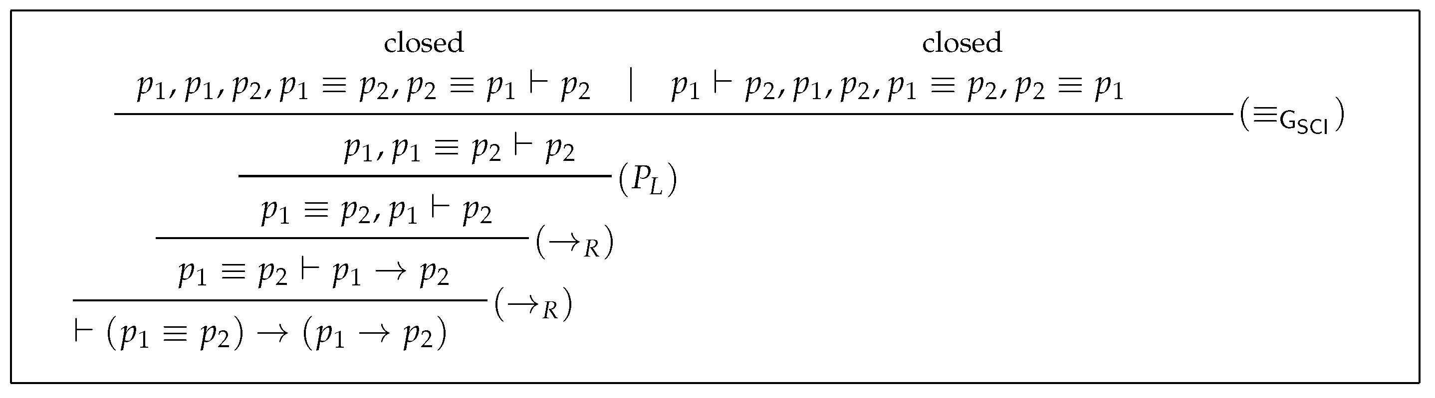
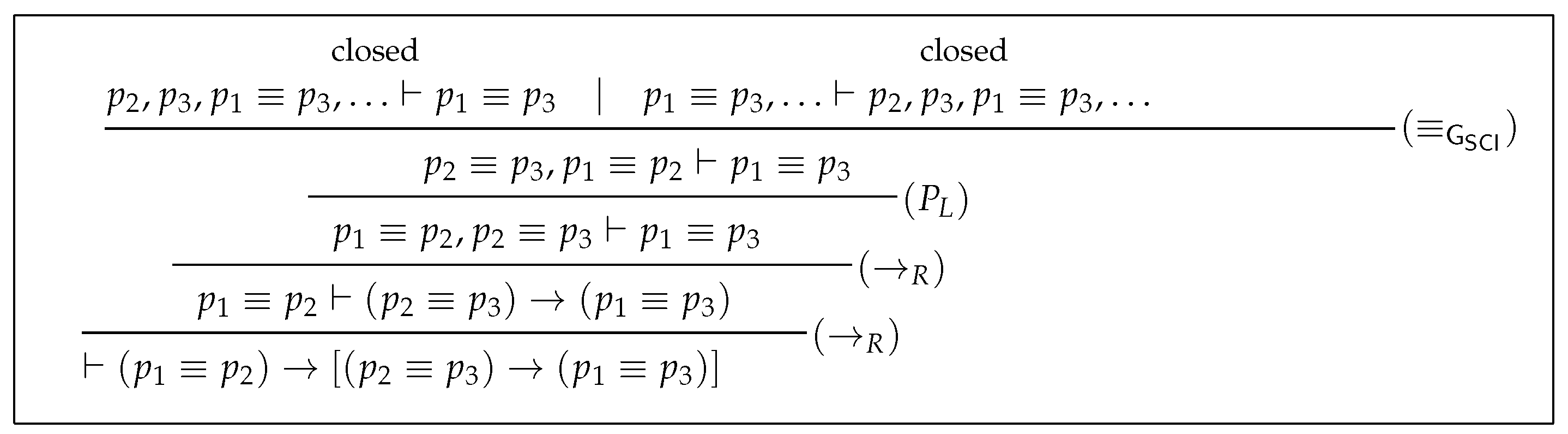
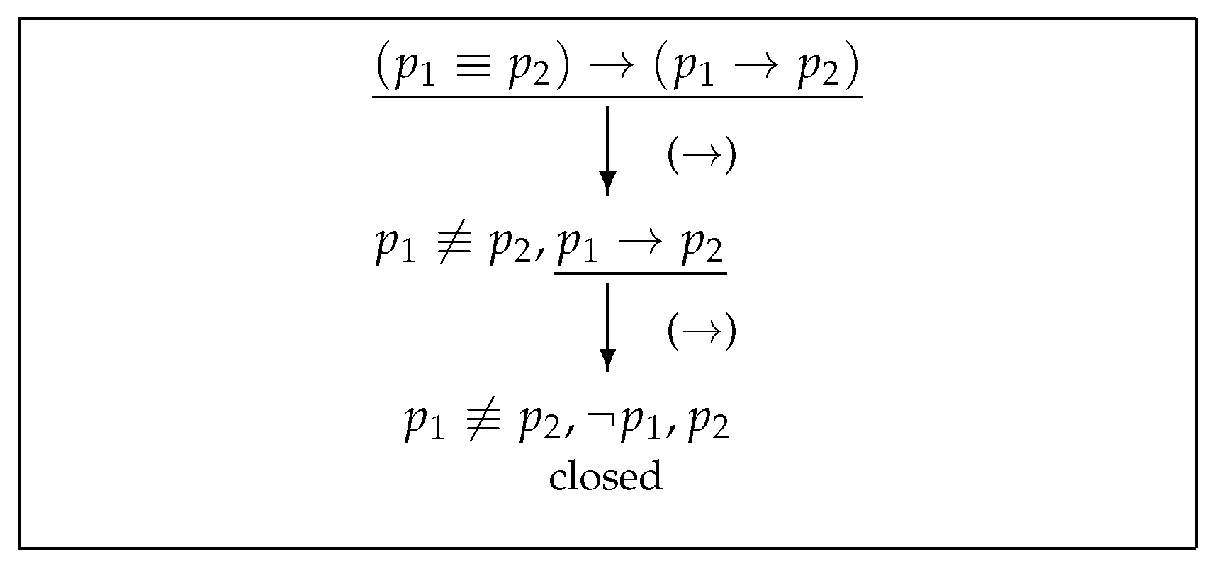
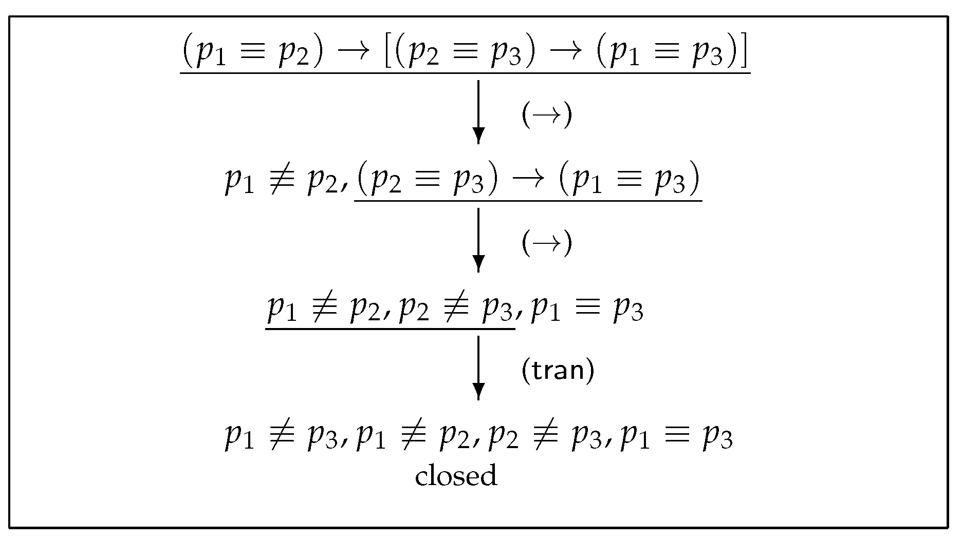
Figure 1 presents a closed ${\mathsf{G}}_{\mathsf{SCI}}$-derivation of the formula $(p_1\equiv p_2)\to (p_1\to p_2)$, which is an instance of the axiom schema $\left({\equiv }_3\right)$, while, in Figure 2, we show how to prove in ${\mathsf{G}}_{\mathsf{SCI}}$ the formula $(p_1\equiv p_2)\to [(p_2\equiv p_3)\to (p_1\equiv p_3)]$, which expresses the fact that the identity connective represents a transitive relation.

4. Dual Tableau System ${\mathsf{DT}}_{\mathsf{SCI}}$

Dual tableau systems are based on Rasiowa–Sikorski diagrams for classical predicate logic (see [17]). They are top–down systems determined by the rules of inferences and axioms. Rules have the following form $\left(\mathsf{rule}\right)$ $\frac{\mathsf{\Phi }}{{\mathsf{\Phi }}_1|\dots |{\mathsf{\Phi }}_n}$, $n\ge 1$, where $\mathsf{\Phi }$, ${\mathsf{\Phi }}_1$, …, ${\mathsf{\Phi }}_n$ are finite sets of formulas. The set $\mathsf{\Phi }$ is called the premise of the rule. Sets ${\mathsf{\Phi }}_1$, …, ${\mathsf{\Phi }}_n$ are said to be conclusions. Some systems allow infinitary rules with infinitely countable many conclusions. The rules are supposed to preserve the validity of the sets of formulas to which they are applied, where the validity of a finite set of formulas is understood as the validity of the disjunction of its elements. Thus, a comma in the sets of a rule $\left(\mathsf{rule}\right)$ can be interpreted as the meta-disjunction, while branching ‘|’ as the meta-conjunction. The rules apply to finite sets of formulas. A rule $\left(\mathsf{rule}\right)$ is applicable to a finite set X, whenever $X=\mathsf{\Phi }$, and there is $i\in \{1,\dots ,n\}$ such that $X\ne {\mathsf{\Phi }}_i$. Axioms are distinguished valid sets of formulas, also referred to as axiomatic sets. The key notion in the methodology of dual tableau systems is a proof tree. A proof tree for a formula $\phi$ is a (finitely) branching tree whose root consists of the set $\left\{\phi \right\}$ and each node of the tree, except the root, is obtained by an application of a rule to its predecessor node. A formula $\phi$ is said to be provable, whenever there is a proof tree for $\phi$ such that all of its branches ends with an axiom.

Dual tableau systems are validity checkers that are in order to prove a formula $\phi$ we build a proof tree directly for that formula. It distinguishes dual tableaux from tableau systems, which are unsatisfiability checkers, as in tableau systems in order to prove a formula a proof tree for its negation is constructed.

Over the years, dual tableaux have been constructed for a great variety of logics, in particular for modal, intuitionistic, relevant, many-valued, temporal, spatial, fuzzy, dynamic programming logics, among others. A very recent comprehensive survey on the foundations and applications of dual tableaux is the book [16].

The first sound and complete dual tableau for the fragment of $\mathsf{SCI}$-language was presented in [15]. A dual tableau for the full $\mathsf{SCI}$-language is described in [16]. The system presented in [15] (resp. [16]) was defined for $\mathsf{SCI}$-language which among its classical connectives contains ¬, ∧, and ∨ (resp. ¬, ∧, ∨, →, ↔). In this section, we present the basics of a dual tableau from [16] adjusted to $\mathsf{SCI}$-language that contains only three connectives ¬, →, and ≡. For the simplicity of our presentation, we will write $\phi \not\equiv \psi$ instead of $\neg (\phi \equiv \psi )$.

The dual tableau system for $\mathsf{SCI}$, denoted by ${\mathsf{DT}}_{\mathsf{SCI}}$, consists of ${\mathsf{DT}}_{\mathsf{SCI}}$-axiomatic sets, decomposition rules $(\neg )$, $(\to )$, $(\neg \to )$ presented in

Table 4. ${\mathsf{DT}}_{\mathsf{SCI}}$-decomposition rules.

(→)   ${\displaystyle \frac{\{\phi \to \psi \}\cup X}{\{\neg \phi ,\psi \}\cup X}}$       ($\neg \to$)    ${\displaystyle \frac{\{\neg (\phi \to \psi \left)\right\}\cup X}{\left\{\phi \right\}\cup X\left|\right\{\neg \psi \}\cup X}}$

(¬)    ${\displaystyle \frac{\{\neg \neg \phi \}\cup X}{\left\{\phi \right\}\cup X}}$

where $\phi$ and $\psi$ are any $\mathsf{SCI}$-formulas,

and X is a finite (possibly empty) set of $\mathsf{SCI}$-formulas.

, and the specific rule $(\equiv )$ depicted in

Table 5. ${\mathsf{DT}}_{\mathsf{SCI}}$-specific rule for the identity connective ≡.

(≡)    ${\displaystyle \frac{\left\{\phi \right(\psi \left)\right\}\cup X}{\{\psi \equiv \vartheta ,\phi (\psi \left)\right\}\cup X\left|\right\{\phi (\psi /\vartheta ),\phi \left(\psi \right)\}\cup X}}$

where $\phi$ and $\vartheta$ are any $\mathsf{SCI}$-formulas, $\psi$ is any subformula of $\phi$,

$\phi \left(\vartheta \right)$ is obtained from $\phi \left(\psi \right)$ by replacing some occurrences of $\psi$ with $\vartheta$

and X is a finite (possibly empty) set of $\mathsf{SCI}$-formulas.

. Decomposition rules enable us to decompose formulas built by means of the classical connectives ¬ and →, while the specific rule reflects properties of the identity connective ≡. ${\mathsf{DT}}_{\mathsf{SCI}}$-axiomatic sets have either of the following forms, where $\phi$ is an $\mathsf{SCI}$-formula and X is a finite (possible empty) set of $\mathsf{SCI}$-formulas: $\{\phi \equiv \phi \}\cup X$ or $\{\phi ,\neg \phi \}\cup X$.

A finite set of $\mathsf{SCI}$-formulas $\{{\phi }_1,\dots ,{\phi }_n\}$ is said to be $\mathsf{SCI}$-valid whenever the disjunction of its elements is $\mathsf{SCI}$-valid that is for every $\mathsf{SCI}$-model $\mathcal{M}$ and for every valuation v in $\mathcal{M}$ there exists $i\in \{1,\dots ,n\}$ such that $\mathcal{M},v\models {\phi }_i$. A ${\mathsf{DT}}_{\mathsf{SCI}}$-proof tree for an $\mathsf{SCI}$-formula $\phi$ is a finitely branching tree whose nodes are sets of formulas satisfying the following conditions:

• the formula $\phi$ is at the root of this tree,
• each node except the root is obtained by an application of a ${\mathsf{DT}}_{\mathsf{SCI}}$-rule to its predecessor node,
• a node does not have successors whenever it is a ${\mathsf{DT}}_{\mathsf{SCI}}$-axiomatic set or none of the rules applies to its set of formulas.

A branch of a ${\mathsf{DT}}_{\mathsf{SCI}}$-proof tree is said to be closed whenever it contains a node with a ${\mathsf{DT}}_{\mathsf{SCI}}$-axiomatic set of formulas. A ${\mathsf{DT}}_{\mathsf{SCI}}$-proof tree is closed whenever all of its branches are closed. A formula $\phi$ is ${\mathsf{DT}}_{\mathsf{SCI}}$-provable whenever there is a closed ${\mathsf{DT}}_{\mathsf{SCI}}$-proof tree for $\phi$, which is then referred to as its ${\mathsf{DT}}_{\mathsf{SCI}}$-proof.

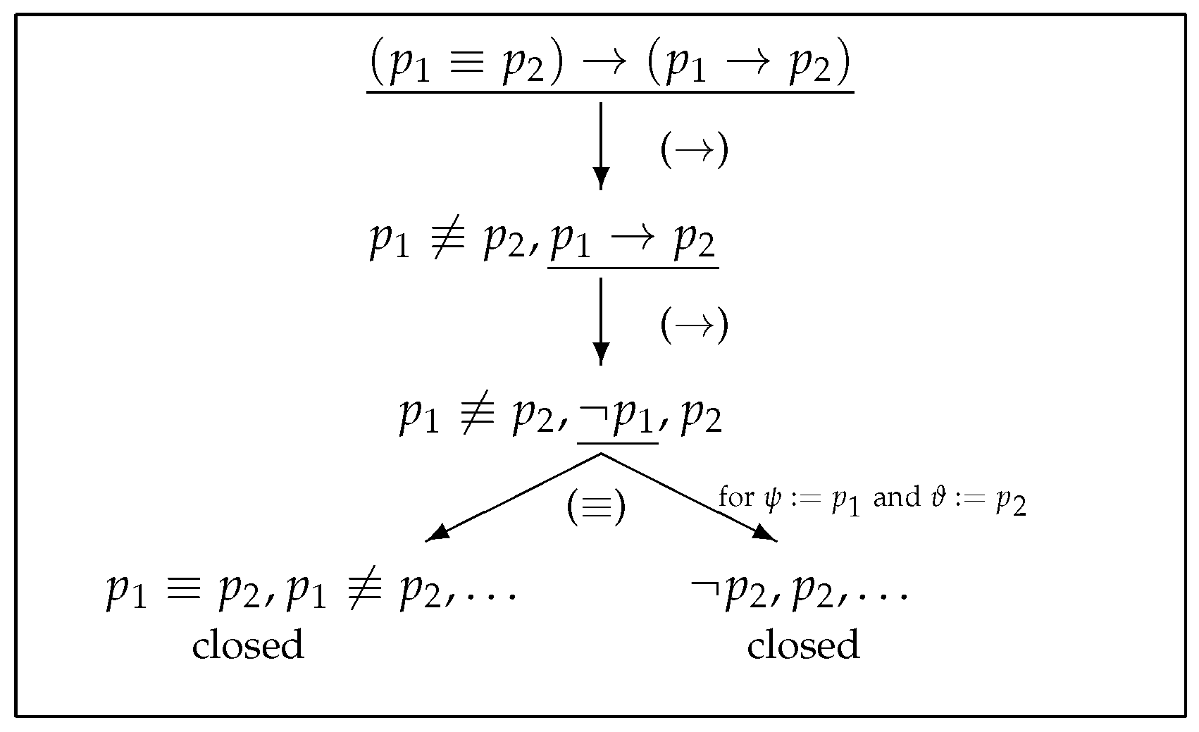
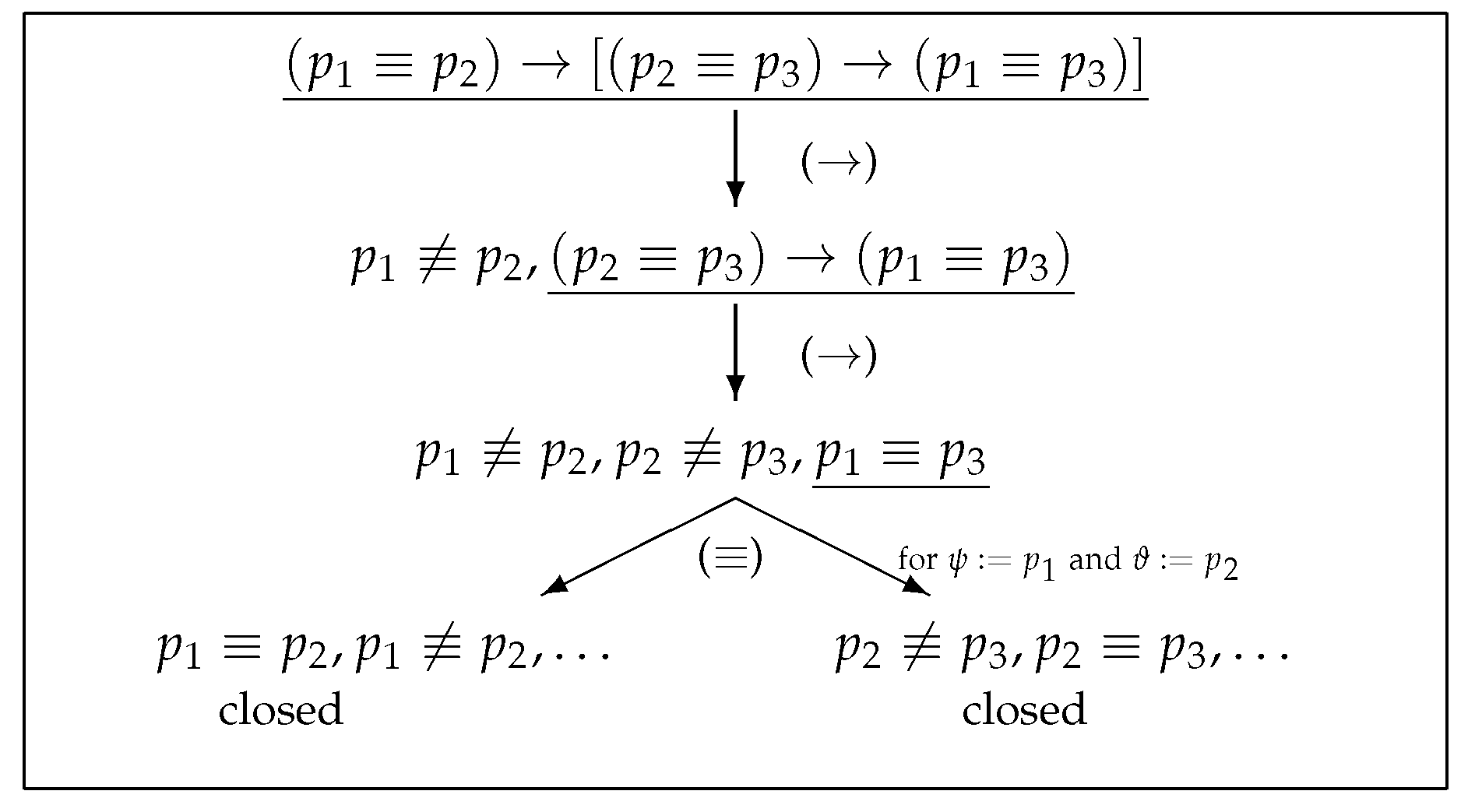
Figure 3 presents a ${\mathsf{DT}}_{\mathsf{SCI}}$-proof for the formula $(p_1\equiv p_2)\to (p_1\to p_2)$, which is an instance of the axiom schema $\left({\equiv }_3\right)$. Figure 4 presents a closed ${\mathsf{DT}}_{\mathsf{SCI}}$-proof tree for the formula $(p_1\equiv p_2)\to [(p_2\equiv p_3)\to (p_1\equiv p_3)]$. In each node of the proof tree, we underline the formula to which a rule has been applied during the construction of the proof tree, and we indicate only those formulas in a node which are essential for this construction.

The proof of soundness and completeness of ${\mathsf{DT}}_{\mathsf{SCI}}$-system is presented in [16] (cf. [15]):

Theorem 4

(Soundness and Completeness of ${\mathsf{DT}}_{\mathsf{SCI}}$). Let φ be an $\mathsf{SCI}$-formula. Then, the following conditions are equivalent:

1.

φ is $\mathsf{SCI}$-valid;

2.

φ is ${\mathsf{DT}}_{\mathsf{SCI}}$-provable.

As in ${\mathsf{G}}_{\mathsf{SCI}}$-system, the rule for the identity connective of the system ${\mathsf{DT}}_{\mathsf{SCI}}$ branches a tree and involves use of substitution. In the next section, we present a new dual tableau that has no such disadvantages.

5. A Substitution-Free Dual Tableau for $\mathsf{SCI}$

In this section, we present the system ${\mathsf{DT}}_{\mathsf{SCI}}^{*}$, which is a modification of ${\mathsf{DT}}_{\mathsf{SCI}}$-system by replacing the rule $(\equiv )$ with several rules for the identity connective that do not involve substitutions. The system ${\mathsf{DT}}_{\mathsf{SCI}}^{*}$ consists of ${\mathsf{DT}}_{\mathsf{SCI}}$-decomposition rules presented in Table 4 (see Section 4) and the specific rules presented in

Table 6. ${\mathsf{DT}}_{\mathsf{SCI}}^{*}$-specific rules for the identity connective.

($\mathsf{ref}$)   ${\displaystyle \frac{X}{\{\phi \not\equiv \phi \}\cup X}}$       ($\mathsf{sym}$)    ${\displaystyle \frac{\{\phi \not\equiv \psi \}\cup X}{\{\psi \not\equiv \phi ,\phi \not\equiv \psi \}\cup X}}$

($\mathsf{tran}$)    ${\displaystyle \frac{\{\phi \not\equiv \psi ,\psi \not\equiv \vartheta \}\cup X}{\{\phi \not\equiv \vartheta ,\phi \not\equiv \psi ,\psi \not\equiv \vartheta \}\cup X}}$

(${\equiv }_{\neg }$)   ${\displaystyle \frac{\{\phi \not\equiv \psi \}\cup X}{\{\neg \phi \not\equiv \neg \psi ,\phi \not\equiv \psi \}\cup X}}$

(${\equiv }_{\to }$)    ${\displaystyle \frac{\{\phi \not\equiv \psi ,\vartheta \not\equiv \chi \}\cup X}{\left\{\right(\phi \to \vartheta )\not\equiv (\psi \to \chi ),\phi \not\equiv \psi ,\vartheta \not\equiv \chi \}\cup X}}$

(${\equiv }_{\equiv }$)    ${\displaystyle \frac{\{\phi \not\equiv \psi ,\vartheta \not\equiv \chi \}\cup X}{\left\{\right(\phi \equiv \vartheta )\not\equiv (\psi \equiv \chi ),\phi \not\equiv \psi ,\vartheta \not\equiv \chi \}\cup X}}$

where $\phi ,\psi ,\vartheta ,\chi$ are any $\mathsf{SCI}$-formulas,

and X is a finite (possibly empty) set of $\mathsf{SCI}$-formulas.

. The specific rule $\left(\mathsf{ref}\right)$ (resp. $\left(\mathsf{sym}\right)$, $\left(\mathsf{tran}\right)$) expresses reflexivity (resp. symmetry, transitivity) of a relation which in $\mathsf{SCI}$-models corresponds to the identity connective. Thus, specific rules $\left(\mathsf{ref}\right)$, $\left(\mathsf{sym}\right)$, and $\left(\mathsf{tran}\right)$ reflect the fact that the relation corresponding to the identity connective is an equivalence relation. The specific rule $\left({\equiv }_{\neg }\right)$ (resp. $\left({\equiv }_{\to }\right)$, $\left({\equiv }_{\equiv }\right)$) expresses the instance of $\mathsf{SCI}$-axiom $\left({\equiv }_2\right)$ (resp. $\left({\equiv }_4\right)$ for → and $\left({\equiv }_4\right)$ for ≡) presented in Section 2. Therefore, specific rules $\left({\equiv }_{\neg }\right)$, $\left({\equiv }_{\to }\right)$, and $\left({\equiv }_{\equiv }\right)$ correspond to the extensionality property for connectives ¬, →, and ≡ (see Proposition 1). As the identity connective can be characterized as an operation that satisfies the extensionality property and represents an equivalence relation, we will show that specific rules $\left(\mathsf{ref}\right)$, $\left(\mathsf{sym}\right)$, $\left(\mathsf{tran}\right)$, $\left({\equiv }_{\neg }\right)$, $\left({\equiv }_{\to }\right)$, and $\left({\equiv }_{\equiv }\right)$ are sufficient to prove completeness of the system ${\mathsf{DT}}_{\mathsf{SCI}}^{*}$.

The axiomatic sets of ${\mathsf{DT}}_{\mathsf{SCI}}^{*}$ have either of the following forms, where $\phi ,\psi$ are any $\mathsf{SCI}$-formulas and X is a finite (possible empty) set of $\mathsf{SCI}$-formulas:

$\left({\mathsf{Ax}}_{{\mathsf{DT}}_{\mathsf{SCI}}^{*}}^1\right)$$\{\phi \equiv \phi \}\cup X$,	$\left({\mathsf{Ax}}_{{\mathsf{DT}}_{\mathsf{SCI}}^{*}}^2\right)$$\{\phi ,\neg \phi \}\cup X$,
$\left({\mathsf{Ax}}_{{\mathsf{DT}}_{\mathsf{SCI}}^{*}}^3\right)$$\{\phi ,\neg \psi ,\phi \not\equiv \psi \}\cup X$,	$\left({\mathsf{Ax}}_{{\mathsf{DT}}_{\mathsf{SCI}}^{*}}^4\right)$$\{\neg \phi ,\psi ,\phi \not\equiv \psi \}\cup X$.

The notions of an $\mathsf{SCI}$-valid set of formulas, a ${\mathsf{DT}}_{\mathsf{SCI}}^{*}$-proof tree, a closed branch of such a tree, a closed ${\mathsf{DT}}_{\mathsf{SCI}}^{*}$-proof tree, and ${\mathsf{DT}}_{\mathsf{SCI}}^{*}$-provability are defined in a similar way as for ${\mathsf{DT}}_{\mathsf{SCI}}$-system in Section 4. Observe that none of the specific rules split a tree or use substitutions.

Now, we will prove the soundness and completeness of ${\mathsf{DT}}_{\mathsf{SCI}}^{*}$-system.

Proposition 3

(Correctness of ${\mathsf{DT}}_{\mathsf{SCI}}^{*}$-rules).For every ${\mathsf{DT}}_{\mathsf{SCI}}^{*}$-rule $\left(\mathsf{rule}\right)$, the premise of $\mathsf{rule}$ is $\mathsf{SCI}$-valid if and only if all of its conclusions are $\mathsf{SCI}$-valid.

Proof. 

The proof for decomposition rules is straightforward, so we will prove the proposition for the specific rules of ${\mathsf{DT}}_{\mathsf{SCI}}^{*}$: $\left(\mathsf{ref}\right)$, $\left(\mathsf{sym}\right)$, $\left(\mathsf{tran}\right)$, $\left({\equiv }_{\neg }\right)$, $\left({\equiv }_{\to }\right)$, $\left({\equiv }_{\equiv }\right)$. Let $\phi ,\psi ,\vartheta ,\chi$ be any $\mathsf{SCI}$-formulas and let X be a finite (possibly empty) set of $\mathsf{SCI}$-formulas. Observe that, in each of the specific ${\mathsf{DT}}_{\mathsf{SCI}}^{*}$-rules, the premise of a rule is a subset of its conclusion. Thus, if the premise is $\mathsf{SCI}$-valid, then so is its conclusion. Therefore, it suffices to show that $\mathsf{SCI}$-validity of the conclusion of a rule implies $\mathsf{SCI}$-validity of its premise.

Correctness of the rule $\left(\mathsf{ref}\right)$

Assume $\{\phi \not\equiv \phi \}\cup X$ is $\mathsf{SCI}$-valid and suppose X is not $\mathsf{SCI}$-valid. Then, there are an $\mathsf{SCI}$-model $\mathcal{M}$ and a valuation v in $\mathcal{M}$ such that, for every $\xi \in X$, $\mathcal{M},v⊭\xi$. Thus, since $\{\phi \not\equiv \phi \}\cup X$ is $\mathsf{SCI}$-valid and $\mathcal{M},v⊭\xi$ for every $\xi \in X$, we obtain $\mathcal{M},v\models \phi \not\equiv \phi$, so $\mathcal{M},v⊭\phi \equiv \phi$. However, all $\mathsf{SCI}$-formulas, $\mathsf{SCI}$-models $\mathcal{M}$, and valuations satisfy $\mathcal{M},v\models \phi \equiv \phi$, a contradiction.

Correctness of the rule $\left(\mathsf{sym}\right)$

Assume that $\{\psi \not\equiv \phi ,\phi \not\equiv \psi \}\cup X$ is $\mathsf{SCI}$-valid and suppose $\{\phi \not\equiv \psi \}\cup X$ is not $\mathsf{SCI}$-valid. Then, there exist an $\mathsf{SCI}$-model $\mathcal{M}$ and a valuation v in $\mathcal{M}$ such that $\mathcal{M},v⊭\phi \not\equiv \psi$ and, for every $\xi \in X$, $\mathcal{M},v⊭\xi$. Thus, $\mathcal{M},v\models \phi \equiv \psi$, which means that $v\left(\phi \right)=v\left(\psi \right)$. Furthermore, by the assumption, the model $\mathcal{M}$ and the valuation v must satisfy the formula $\psi \not\equiv \phi$, so $v\left(\psi \right)\ne v\left(\phi \right)$, a contradiction.

Correctness of the rule $\left(\mathsf{tran}\right)$

Assume $\{\phi \not\equiv \vartheta ,\phi \not\equiv \psi ,\psi \not\equiv \vartheta \}\cup X$ is $\mathsf{SCI}$-valid and suppose $\{\phi \not\equiv \psi ,\psi \not\equiv \vartheta \}\cup X$ is not $\mathsf{SCI}$-valid. Then, there exists an $\mathsf{SCI}$-model $\mathcal{M}$ and a valuation v in $\mathcal{M}$ that do not satisfy any formula from the set $\{\phi \not\equiv \psi ,\psi \not\equiv \vartheta \}\cup X$, so $\mathcal{M},v\models \phi \equiv \psi$ and $\mathcal{M},v\models \psi \equiv \vartheta$. Hence, we obtain $v\left(\phi \right)=v\left(\psi \right)=v\left(\vartheta \right)$. However, by the assumption, it must hold that $\mathcal{M},v\models \phi \not\equiv \vartheta$, which imply $v\left(\phi \right)\ne v\left(\vartheta \right)$, a contradiction.

Correctness of the rule $\left({\equiv }_{\neg }\right)$

Assume $\{\neg \phi \not\equiv \neg \psi ,\phi \not\equiv \psi \}\cup X$ is $\mathsf{SCI}$-valid and suppose $\{\phi \not\equiv \psi \}\cup X$ is not $\mathsf{SCI}$-valid. Then, there exist an $\mathsf{SCI}$-model $\mathcal{M}=(U,\sim ,\Rightarrow ,\circ ,D)$ and a valuation v such that $\mathcal{M},v\models \phi \equiv \psi$ that is $v\left(\phi \right)=v\left(\psi \right)$. On the other hand, by the assumption, $\mathcal{M},v\models \neg \phi \not\equiv \neg \psi$, which imply $v(\neg \phi )\ne v(\neg \psi )$. However, if $v\left(\phi \right)=v\left(\psi \right)$, then clearly $v(\neg \phi )=\sim v\left(\phi \right)=\sim v\left(\psi \right)=v(\neg \psi )$, which contradicts $v(\neg \phi )\ne v(\neg \psi )$.

Correctness of the rule $\left({\equiv }_{\to }\right)$

Assume $\left\{\right(\phi \to \vartheta )\not\equiv (\psi \to \chi ),\phi \not\equiv \psi ,\vartheta \not\equiv \chi \}\cup X$ is $\mathsf{SCI}$-valid and suppose $\{\phi \not\equiv \psi ,\vartheta \not\equiv \chi \}\cup X$ is not $\mathsf{SCI}$-valid. Then, there exist an $\mathsf{SCI}$-model $\mathcal{M}=(U,\sim ,\Rightarrow ,\circ ,D)$ and a valuation v such that $\mathcal{M},v\models \phi \equiv \psi$ and $\mathcal{M},v\models \vartheta \equiv \chi$, that is, $v\left(\phi \right)=v\left(\psi \right)$ and $v\left(\vartheta \right)=v\left(\chi \right)$. Hence, due to the definition of an $\mathsf{SCI}$-model, we obtain: $v(\phi \to \vartheta )=v\left(\phi \right)\Rightarrow v\left(\vartheta \right)=v\left(\psi \right)\Rightarrow v\left(\chi \right)=v(\psi \to \chi )$. Therefore, $\mathcal{M},v\models (\phi \to \vartheta )\equiv (\psi \to \chi )$. However, by the assumption, $\mathcal{M},v\models (\phi \to \vartheta )\not\equiv (\psi \to \chi )$, a contradiction.

Correctness of the rule $\left({\equiv }_{\equiv }\right)$

Assume $\left\{\right(\phi \equiv \vartheta )\not\equiv (\psi \equiv \chi ),\phi \not\equiv \psi ,\vartheta \not\equiv \chi \}\cup X$ is $\mathsf{SCI}$-valid and suppose $\{\phi \not\equiv \psi ,\vartheta \not\equiv \chi \}\cup X$ is not $\mathsf{SCI}$-valid. Then, there exist an $\mathsf{SCI}$-model $\mathcal{M}=(U,\sim ,\Rightarrow ,\circ ,D)$ and a valuation v such that $\mathcal{M},v\models \phi \equiv \psi$ and $\mathcal{M},v\models \vartheta \equiv \chi$ that is $v\left(\phi \right)=v\left(\psi \right)$ and $v\left(\vartheta \right)=v\left(\chi \right)$. Thus, by the definition of an $\mathsf{SCI}$-model, we obtain that $v(\phi \equiv \vartheta )=v\left(\phi \right)\circ v\left(\vartheta \right)=v\left(\psi \right)\circ v\left(\chi \right)=v(\psi \equiv \chi )$, and so $\mathcal{M},v\models (\phi \equiv \vartheta )\equiv (\psi \equiv \chi )$. By the assumption, $\mathcal{M},v\models (\phi \equiv \vartheta )\not\equiv (\psi \equiv \chi )$, a contradiction. □

Proposition 4

(Validity of ${\mathsf{DT}}_{\mathsf{SCI}}^{*}$-axiomatic sets). All the ${\mathsf{DT}}_{\mathsf{SCI}}^{*}$-axiomatic sets are $\mathsf{SCI}$-valid.

Proof. 

Let $\phi$, $\psi$ be any $\mathsf{SCI}$-formulas and let X be any finite (possibly empty) set of $\mathsf{SCI}$-formulas. The proof of validity of sets $\left({\mathsf{Ax}}_{{\mathsf{DT}}_{\mathsf{SCI}}^{*}}^1\right)$ and $\left({\mathsf{Ax}}_{{\mathsf{DT}}_{\mathsf{SCI}}^{*}}^2\right)$ is obvious. By way of example, we will prove validity of sets $\left({\mathsf{Ax}}_{{\mathsf{DT}}_{\mathsf{SCI}}^{*}}^3\right)$, since the proof for $\left({\mathsf{Ax}}_{{\mathsf{DT}}_{\mathsf{SCI}}^{*}}^4\right)$ is similar. Suppose a set $\{\phi ,\neg \psi ,\phi \not\equiv \psi \}\cup X$ is not $\mathsf{SCI}$-valid. Then, there exist an $\mathsf{SCI}$-model $\mathcal{M}=(U,\sim ,\Rightarrow ,\circ ,D)$ and a valuation v such that $\mathcal{M},v⊭\phi$, $\mathcal{M},v⊭\neg \psi$, and $\mathcal{M},v⊭\phi \equiv \psi$. Thus, by the definition of an $\mathsf{SCI}$-model, $v\left(\phi \right)\notin D$, $\sim v\left(\psi \right)\notin D$, and $\sim \left(v\right(\phi )\circ v(\psi \left)\right)\notin D$. However, this means that $v\left(\phi \right)\notin D$, $v\left(\psi \right)\in D$, and $v\left(\phi \right)=v\left(\psi \right)$, which is not possible since the latter implies $v\left(\phi \right)\in D$ iff $v\left(\psi \right)\in D$. □

Due to Propositions 3 and 4, the soundness of ${\mathsf{DT}}_{\mathsf{SCI}}^{*}$ can be easily proved:

Theorem 5

(Soundness of ${\mathsf{DT}}_{\mathsf{SCI}}^{*}$). If an $\mathsf{SCI}$-formula is ${\mathsf{DT}}_{\mathsf{SCI}}^{*}$-provable, then it is $\mathsf{SCI}$-valid.

Proof. 

Let $\phi$ be a ${\mathsf{DT}}_{\mathsf{SCI}}^{*}$-provable formula. Then, there exists a closed ${\mathsf{DT}}_{\mathsf{SCI}}^{*}$-proof tree for $\phi$ that is all of its branches end with ${\mathsf{DT}}_{\mathsf{SCI}}^{*}$-axiomatic sets. By Proposition 4, all ${\mathsf{DT}}_{\mathsf{SCI}}^{*}$-axiomatic sets are $\mathsf{SCI}$-valid, so the leaves in the closed ${\mathsf{DT}}_{\mathsf{SCI}}^{*}$-proof tree for $\phi$ are $\mathsf{SCI}$-valid sets of formulas. Moreover, by Proposition 3, if conclusions of a rule are $\mathsf{SCI}$-valid, then so is its premise. Therefore, going from the leaves to the root of the tree, in each step, we obtain nodes that are $\mathsf{SCI}$-valid. Hence, the root $\left\{\phi \right\}$ is $\mathsf{SCI}$-valid, and so we conclude that the formula $\phi$ is $\mathsf{SCI}$-valid. □

In order to prove completeness of ${\mathsf{DT}}_{\mathsf{SCI}}^{*}$, we will construct an $\mathsf{SCI}$-model and a valuation that do not satisfy a formula, which is not ${\mathsf{DT}}_{\mathsf{SCI}}^{*}$-provable. We call a branch b of a ${\mathsf{DT}}_{\mathsf{SCI}}^{*}$-proof tree ${\mathsf{DT}}_{\mathsf{SCI}}^{*}$-complete whenever it satisfies the following completion conditions for all $\mathsf{SCI}$-formulas $\phi ,\psi ,\vartheta ,\chi$:

Cpl(¬) If $\neg \neg \phi \in b$, then $\phi \in b$.

Cpl(→) If $\phi \to \psi \in b$, then both $\neg \phi \in b$ and $\psi \in b$.

Cpl($\neg \to$) If $\neg (\phi \to \psi )\in b$, then either $\phi \in b$ or $\neg \psi \in b$.

Cpl($\mathsf{ref}$) For every $\mathsf{SCI}$-formula $\phi$, $\phi \not\equiv \phi \in b$.

Cpl($\mathsf{sym}$) If $\phi \not\equiv \psi \in b$, then $\psi \not\equiv \phi \in b$.

Cpl($\mathsf{tran}$) If $\phi \not\equiv \psi \in b$ and $\psi \not\equiv \vartheta \in b$, then $\phi \not\equiv \vartheta \in b$.

Cpl(${\equiv }_{\neg }$) If $\phi \not\equiv \psi \in b$, then $\neg \phi \not\equiv \neg \psi \in b$.

Cpl(${\equiv }_{\to }$) If $\phi \not\equiv \psi \in b$ and $\vartheta \not\equiv \chi \in b$, then $(\phi \to \vartheta )\not\equiv (\psi \to \chi )\in b$.

Cpl(${\equiv }_{\equiv }$) If $\phi \not\equiv \psi \in b$ and $\vartheta \not\equiv \chi \in b$, then $(\phi \equiv \vartheta )\not\equiv (\psi \equiv \chi )\in b$.

A ${\mathsf{DT}}_{\mathsf{SCI}}^{*}$-proof tree is said to be ${\mathsf{DT}}_{\mathsf{SCI}}^{*}$-complete whenever each of its branches is either closed or ${\mathsf{DT}}_{\mathsf{SCI}}^{*}$-complete. The rules of ${\mathsf{DT}}_{\mathsf{SCI}}^{*}$-system guarantee that, for every $\mathsf{SCI}$-formula, there is a complete ${\mathsf{DT}}_{\mathsf{SCI}}^{*}$-proof tree. A non-closed branch that is ${\mathsf{DT}}_{\mathsf{SCI}}^{*}$-complete will be referred to as open. The following property can be easily proved:

Proposition 5

(Closed Branch Property). For every complete branch b of a ${\mathsf{DT}}_{\mathsf{SCI}}^{*}$-proof tree and for every $\mathsf{SCI}$-formula φ, if both $\phi \in b$ and $\neg \phi \in b$, then the branch b is closed.

Proof. 

Let b be a complete branch of ${\mathsf{DT}}_{\mathsf{SCI}}^{*}$-proof tree and let $\phi$ be an $\mathsf{SCI}$-formula such that both $\phi \in b$ and $\neg \phi \in b$. Suppose b is not closed. We will prove the proposition by the induction on complexity of formulas. First, observe that all the ${\mathsf{DT}}_{\mathsf{SCI}}^{*}$-rules preserves propositional variables, negations of propositional variables, identities and negations of identities, that is, if a node contains $\phi$ or $\neg \phi$, for $\phi \in \mathbb{V}\cup \{\psi \equiv \vartheta ;\psi ,\vartheta \in \mathbb{FOR}\}$, then all of its successors contain these formulas. Thus, if $\phi \in b$ and $\neg \phi \in b$, then there exists a node t in branch b such that both $\phi \in t$ and $\neg \phi \in t$, which means that a node t is ${\mathsf{DT}}_{\mathsf{SCI}}^{*}$-axiomatic, and branch b is closed. Hence, the proposition holds for formulas from the set $\mathbb{V}\cup \{\psi \equiv \vartheta ;\psi ,\vartheta \in \mathbb{FOR}\}$. Assume the proposition holds for $\phi$ and $\psi$. We will show that it holds for formulas $\neg \phi$ and $\phi \to \psi$. Assume $\neg \phi \in b$ and $\neg \neg \phi \in b$. Then, as b is a non-closed complete branch and $\neg \neg \phi \in b$, by the completion condition Cpl(¬), $\phi \in b$. Thus, we have $\neg \phi \in b$ and $\phi \in b$, so by the inductive hypothesis, b is closed. Now, let $\phi \to \psi \in b$ and $\neg (\phi \to \psi )\in b$. Since b is a non-closed complete branch and $\phi \to \psi \in b$, by the completion condition Cpl(→), we obtain that both $\neg \phi \in b$ and $\psi \in b$. Similarly, by the completion condition Cpl($\neg \to$), we have that either $\phi \in b$ or $\neg \psi \in b$. Therefore, either both $\phi \in b$ and $\neg \phi \in b$ or both $\psi \in b$ and $\neg \psi \in b$. Hence, by the inductive hypothesis, the branch b must be closed, which ends the proof. □

Let b be an open branch of a ${\mathsf{DT}}_{\mathsf{SCI}}^{*}$-proof tree and let $R_{\circ }$ be defined on the set of all $\mathsf{SCI}$-formulas as follows:

$$(\phi ,\psi )\in R_{\circ }\stackrel{\mathrm{df}}{⟺}(\phi \not\equiv \psi )\in b.$$

Proposition 6.

For every open branch b of a ${\mathsf{DT}}_{\mathsf{SCI}}^{*}$-proof tree, $R_{\circ }$ is an equivalence relation on the set of all $\mathsf{SCI}$-formulas.

Proof. 

Let b be an open branch of a ${\mathsf{DT}}_{\mathsf{SCI}}^{*}$-proof tree and let $\phi$ be an $\mathsf{SCI}$-formula. Then, by the completion condition Cpl($\mathsf{ref}$), $\phi \not\equiv \phi$ belongs to the branch b, and so $(\phi ,\phi )\in R_{\circ }$, that is, $R_{\circ }$ is reflexive. Assume $\phi$ and $\psi$ are $\mathsf{SCI}$-formulas such that $(\phi ,\psi )\in R_{\circ }$. Then, $\phi \not\equiv \psi \in b$, and by the completion condition Cpl($\mathsf{sym}$), $\psi \not\equiv \phi \in b$. Thus, $(\psi ,\phi )\in R_{\circ }$, which means that $R_{\circ }$ is symmetric. Now, assume that $(\phi ,\psi )\in R_{\circ }$ and $(\psi ,\vartheta )\in R_{\circ }$, that is, both formulas $\phi \not\equiv \psi$ and $\psi \not\equiv \vartheta$ are in b. Therefore, by the completion condition Cpl($\mathsf{tran}$), $\phi \not\equiv \vartheta \in b$, so $(\phi ,\vartheta )\in R_{\circ }$. Thus, the relation $R_{\circ }$ is transitive. Hence, we have proved that $R_{\circ }$ is an equivalence relation. □

Proposition 7.

For every open branch b of a ${\mathsf{DT}}_{\mathsf{SCI}}^{*}$-proof tree, the relation $R_{\circ }$ is compatible with all the connectives of $\mathsf{SCI}$.

Proof. 

Let b be an open branch of a ${\mathsf{DT}}_{\mathsf{SCI}}^{*}$-proof tree and let $\phi ,\psi ,\vartheta ,\chi$ be $\mathsf{SCI}$-formulas. Assume $(\phi ,\psi )\in R_{\circ }$, that is, $\phi \not\equiv \psi \in b$. Then, due to the completion condition Cpl(${\equiv }_{\neg }$), $\neg \phi \not\equiv \neg \psi \in b$, so $(\neg \phi ,\neg \psi )\in R_{\circ }$. Thus, $R_{\circ }$ is compatible with ¬. Now, let $(\phi ,\psi )\in R_{\circ }$ and $(\vartheta ,\chi )\in R_{\circ }$, that is, $\phi \not\equiv \psi \in b$ and $\vartheta \not\equiv \chi \in b$. Then, by the completion condition Cpl(${\equiv }_{\to }$), we obtain $(\phi \to \vartheta )\not\equiv (\psi \to \chi )\in b$, that is, $((\phi \to \vartheta ),(\psi \to \chi ))\in R_{\circ }$, so $R_{\circ }$ is compatible with →. Finally, assume that $(\phi ,\psi )\in R_{\circ }$ and $(\vartheta ,\chi )\in R_{\circ }$, that is, $\phi \not\equiv \psi \in b$ and $\vartheta \not\equiv \chi \in b$. Then, by the completion condition Cpl(${\equiv }_{\equiv }$), we have $(\phi \equiv \vartheta )\not\equiv (\psi \equiv \chi )\in b$, that is, $((\phi \equiv \vartheta ),(\psi \equiv \chi ))\in R_{\circ }$, so $R_{\circ }$ is compatible with ≡, which ends the proof. □

Let $p\in \mathbb{V}$ and let $\phi ,\psi$ be $\mathsf{SCI}$-formulas. We define the depth of an $\mathsf{SCI}$-formula as follows:

$d\left(p\right)=d(\phi \equiv \psi )=0$$d(\neg \phi )=d\left(\phi \right)+1$$d(\phi \to \psi )=max\left(d\right(\phi ),d(\psi \left)\right)+1$.

By ${\mathbb{FOR}}^n$, we denote the set of all $\mathsf{SCI}$-formulas of depth n. Given an $\mathsf{SCI}$-formula $\phi$, by ${\left[\phi \right]}_{R_{\circ }}$ we denote the equivalence class of $R_{\circ }$ determined by $\phi$. Let b be an open branch of a ${\mathsf{DT}}_{\mathsf{SCI}}^{*}$-proof tree and let ${\mathcal{M}}^b=(U^b,{\sim }^b,{\Rightarrow }^b,{\circ }^b,D^b)$ be the branch structure defined as follows:

• $U^b=\{{\left[\phi \right]}_{R_{\circ }}:\phi \in \mathbb{FOR}\}$,
• $D^b=\{{\left[\phi \right]}_{R_{\circ }}:\phi \in {\bigcup }_{n\in \mathbb{N}}{D}_n\}$, where
  • $D_0=\{\phi \in {\mathbb{FOR}}^0:\neg \phi \in b\}$,
  • $D_{n+1}=D_{n+1}^1\cup D_{n+1}^2$, for
    $D_{n+1}^1=\{\neg \phi \in {\mathbb{FOR}}^{n+1}:\phi \notin D_n\}$
    $D_{n+1}^2=\{\phi \to \psi \in {\mathbb{FOR}}^{n+1}:\phi \notin {\bigcup }_{k\le n}{D}_{k}or\psi \in {\bigcup }_{k\le n}{D}_k)\}$,
• operations ${\sim }^b$, ${\Rightarrow }^b$, ${\circ }^b$ are defined as:
  ${\sim }^b{\left[\phi \right]}_{R_{\circ }}\stackrel{\mathrm{df}}{=}{[\neg \phi ]}_{R_{\circ }}$${\left[\phi \right]}_{R_{\circ }}{\Rightarrow }^b{\left[\psi \right]}_{R_{\circ }}\stackrel{\mathrm{df}}{=}{[\phi \to \psi ]}_{R_{\circ }}$${\left[\phi \right]}_{R_{\circ }}{\circ }^b{\left[\psi \right]}_{R_{\circ }}=\stackrel{\mathrm{df}}{=}{[\phi \equiv \psi ]}_{R_{\circ }}$.

Proposition 8

(Branch Model Property). For every open branch b of a ${\mathsf{DT}}_{\mathsf{SCI}}^{*}$-proof tree, the branch structure ${\mathcal{M}}^b$ is an $\mathsf{SCI}$-model.

Proof. 

Let b be an open branch of a ${\mathsf{DT}}_{\mathsf{SCI}}^{*}$-proof tree. Clearly, $U^b$ is not empty. Observe also that, for every formula $\phi \in {\mathbb{FOR}}^n$, it holds that $\phi \in {\bigcup }_{n\in \mathbb{N}}{D}_n$ iff $\phi \in D_n$. Hence, for every formula $\phi \in {\mathbb{FOR}}^n$, ${\left[\phi \right]}_{R_{\circ }}\in D^b$ iff $\phi \in D_n$. Moreover, by the completion condition Cpl($\mathsf{ref}$), for every $\mathsf{SCI}$-formula $\phi$, $\phi \not\equiv \phi \in b$, which means that $\phi \equiv \phi \in D_0$, and so ${[\phi \equiv \phi ]}_{R_{\circ }}\in D^b$. Thus, $D^b\ne \varnothing$. Now, as $\phi \equiv \phi \in D_0$ and $\phi \not\equiv \phi \in {\mathbb{FOR}}^1$, by the definition of $D_n$, $\phi \not\equiv \phi \notin D_1$, and so ${[\phi \not\equiv \phi ]}_{R_{\circ }}\notin D^b$. Thus, $U^b\setminus D^b\ne \varnothing$.

Due to Proposition 7, operations ${\sim }^b$, ${\Rightarrow }^b$, and ${\circ }^b$ are well defined. Indeed, assume ${\left[\phi \right]}_{R_{\circ }}={\left[\psi \right]}_{R_{\circ }}$, that is, $(\phi ,\psi )\in R_{\circ }$. Then, by Proposition 7, $(\neg \phi ,\neg \psi )\in R_{\circ }$, and so ${[\neg \phi ]}_{R_{\circ }}={[\neg \psi ]}_{R_{\circ }}$. Thus, since ${\sim }^b{\left[\phi \right]}_{R_{\circ }}={[\neg \phi ]}_{R_{\circ }}$ and ${\sim }^b{\left[\psi \right]}_{R_{\circ }}={[\neg \psi ]}_{R_{\circ }}$, we get ${\sim }^b{\left[\phi \right]}_{R_{\circ }}={\sim }^b{\left[\psi \right]}_{R_{\circ }}$. Therefore, if ${\left[\phi \right]}_{R_{\circ }}={\left[\psi \right]}_{R_{\circ }}$, then ${\sim }^b{\left[\phi \right]}_{R_{\circ }}={\sim }^b{\left[\psi \right]}_{R_{\circ }}$. Now, let $\#\in \{\to ,\equiv \}$ and let ${\#}^b$ be defined as: ${\#}^b={\Rightarrow }^b$, if $\#=\to$; and ${\#}^b={\circ }^b$ otherwise. Assume ${\left[\phi \right]}_{R_{\circ }}={\left[\psi \right]}_{R_{\circ }}$ and ${\left[\vartheta \right]}_{R_{\circ }}={\left[\chi \right]}_{R_{\circ }}$, that is, $(\phi ,\psi )\in R_{\circ }$ and $(\vartheta ,\chi )\in R_{\circ }$. By Proposition 7, we obtain that $((\phi \#\vartheta ),(\psi \#\chi ))\in R_{\circ }$, and so ${[\phi \#\vartheta ]}_{R_{\circ }}={[\psi \#\chi ]}_{R_{\circ }}$. Therefore, we have:

${\left[\phi \right]}_{R_{\circ }}{\#}^b{\left[\vartheta \right]}_{R_{\circ }}={[\phi \#\vartheta ]}_{R_{\circ }}={[\psi \#\chi ]}_{R_{\circ }}={\left[\psi \right]}_{R_{\circ }}{\#}^b{\left[\chi \right]}_{R_{\circ }}.$

Hence, operations ${\sim }^b$, ${\Rightarrow }^b$, and ${\circ }^b$ are well defined. Now, we will prove that they satisfy semantic conditions with respect to $D^b$. Note that $D^b$ satisfy the following properties for every $\mathsf{SCI}$-formula $\phi$ and for all $n,k\in \mathbb{N}$:

(*)	If $d\left(\phi \right)=n$, then ${\left[\phi \right]}_{R_{\circ }}\in D^b$ iff $\phi \in D_n$.
(**)	If $\phi \in D_n$, then $d\left(\phi \right)=n$.
(***)	If $d\left(\phi \right)=n$ and $k\ne n$, then $\phi \notin D_k$.

Let ${\left[\phi \right]}_{R_{\circ }}\in U^b$ be such that $d\left(\phi \right)=n$, for some $n\in \mathbb{N}$. Assume ${\sim }^b{\left[\phi \right]}_{R_{\circ }}\in D^b$, which by the definition of the operation ${\sim }^b$ means that ${[\neg \phi ]}_{R_{\circ }}\in D^b$. Thus, since $d(\neg \phi )=n+1$, by (*), we have $\neg \phi \in D_{n+1}$. Then, by the definition of $D^b$, it holds that $\phi \notin D_n$, and thus due to (*) we obtain that ${\left[\phi \right]}_{R_{\circ }}\notin D^b$. Now, assume that ${\left[\phi \right]}_{R_{\circ }}\notin D^b$, that is, by (*), we obtain $\phi \notin D_n$. Thus, by the definition of $D^b$, we get $\neg \phi \in D_{n+1}$, which due to (*) means that ${[\neg \phi ]}_{R_{\circ }}\in D^b$. Hence, by the definition of the operation ${\sim }^b$, we have ${\sim }^b{\left[\phi \right]}_{R_{\circ }}\in D^b$. Therefore, we have proved that ${\sim }^b{\left[\phi \right]}_{R_{\circ }}\in D^b$ iff ${\left[\phi \right]}_{R_{\circ }}\notin D^b$.

Let ${\left[\phi \right]}_{R_{\circ }},{\left[\psi \right]}_{R_{\circ }}\in U^b$. Assume ${\left[\phi \right]}_{R_{\circ }}{\Rightarrow }^b{\left[\psi \right]}_{R_{\circ }}\in D^b$. Then, by the definition of ${\Rightarrow }^b$, ${[\phi \to \psi ]}_{R_{\circ }}\in D^b$. By the definition of $D^b$, there exists $n\in \mathbb{N}$ such that $\phi \to \psi \in D_n$, which, by (**), implies $d(\phi \to \psi )=n$, and clearly $n\ge 1$. Since $\phi \to \psi \in D_n$, by the definition of $D^b$, we obtain that either $\phi \notin {\bigcup }_{k<n}{D}_k$ or $\psi \in {\bigcup }_{k<n}{D}_k$. Clearly, $d\left(\phi \right)<n$, so, if $\phi \notin {\bigcup }_{k<n}{D}_k$, then, due to (*), we get ${\left[\phi \right]}_{R_{\circ }}\notin D^b$. Moreover, $d\left(\psi \right)<n$, so, if $\psi \in {\bigcup }_{k<n}{D}_k$, then, by (*), it holds that ${\left[\psi \right]}_{R_{\circ }}\in D^b$. Hence, we have proved that, if ${\left[\phi \right]}_{R_{\circ }}{\Rightarrow }^b{\left[\psi \right]}_{R_{\circ }}\in D^b$, then either ${\left[\phi \right]}_{R_{\circ }}\notin D^b$ or ${\left[\psi \right]}_{R_{\circ }}\in D^b$. Now, let us assume that $d\left(\phi \right)=i$, $d\left(\psi \right)=j$, for some $i,j\in \mathbb{N}$, and either ${\left[\phi \right]}_{R_{\circ }}\notin D^b$ or ${\left[\psi \right]}_{R_{\circ }}\in D^b$. Thus, by (**), $\phi \notin D_i$ or $\psi \in D_j$. Let $n=max(i,j)+1$. If $\phi \notin D_i$, then, by (***), it can be easily proved that $\phi \notin {\bigcup }_{k<n}{D}_k$. If $\psi \in D_j$, then, by (*), $\psi \in {\bigcup }_{k<n}{D}_k$. Therefore, either $\phi \notin {\bigcup }_{k<n}{D}_k$ or $\psi \in {\bigcup }_{k<n}{D}_k$. Then, by the definition of $D^b$, it follows that $\phi \to \psi \in D_n$, and, by (*), we have ${[\phi \to \psi ]}_{R_{\circ }}\in D^b$. Thus, by the definition of the operation ${\Rightarrow }^b$, we obtain that ${\left[\phi \right]}_{R_{\circ }}{\Rightarrow }^b{\left[\psi \right]}_{R_{\circ }}\in D^b$. Hence, we have proved that ${\left[\phi \right]}_{R_{\circ }}{\Rightarrow }^b{\left[\psi \right]}_{R_{\circ }}\in D^b$ iff either ${\left[\phi \right]}_{R_{\circ }}\notin D^b$ or ${\left[\psi \right]}_{R_{\circ }}\in D^b$.

Now, let ${\left[\phi \right]}_{R_{\circ }},{\left[\psi \right]}_{R_{\circ }}\in U^b$. Clearly, $d(\phi \equiv \psi )=0$. Then, the following can be easily shown:

${\left[\phi \right]}_{R_{\circ }}{\circ }^b{\left[\psi \right]}_{R_{\circ }}\in D^b$ iff ${[\phi \equiv \psi ]}_{R_{\circ }}\in D^b$ iff $\phi \equiv \psi \in D_0$ iff $\phi \not\equiv \psi \in b$ iff $(\phi ,\psi )\in R_{\circ }$ iff ${\left[\phi \right]}_{R_{\circ }}={\left[\psi \right]}_{R_{\circ }}$.

Hence, we have shown that ${\left[\phi \right]}_{R_{\circ }}{\circ }^b{\left[\psi \right]}_{R_{\circ }}\in D^b$ iff ${\left[\phi \right]}_{R_{\circ }}={\left[\psi \right]}_{R_{\circ }}$. Therefore, we have proved that the branch structure ${\mathcal{M}}^b$ is an $\mathsf{SCI}$-model. □

Let ${\mathcal{M}}^b=(U^b,{\sim }^b,{\Rightarrow }^b,{\circ }^b,D^b)$ be the branch structure for an open branch b of a ${\mathsf{DT}}_{\mathsf{SCI}}^{*}$-proof tree. Let $v^b:\mathbb{FOR}\to U^b$ be a function such that $v^b\left(\phi \right)={\left[\phi \right]}_{R_{\circ }}$, for all $\phi \in \mathbb{FOR}$. Due to the definition of ${\mathcal{M}}^b$, the following can be easily proved:

Proposition 9.

Let b be an open branch of a ${\mathsf{DT}}_{\mathsf{SCI}}^{*}$-proof tree and let ${\mathcal{M}}^b=(U^b,{\sim }^b,{\Rightarrow }^b,{\circ }^b,D^b)$ be the branch structure. Then, the function $v^b:\mathbb{FOR}\to U^b$ such that $v^b\left(\phi \right)={\left[\phi \right]}_{R_{\circ }}$, for all $\phi \in \mathbb{FOR}$, is an $\mathsf{SCI}$-valuation in ${\mathcal{M}}^b$, that is, for all $\mathsf{SCI}$-formulas φ and ψ, the following hold:

$v^b(\neg \phi )={\sim }^b{\left[\phi \right]}_{R_{\circ }}$$v^b(\phi \to \psi )={\left[\phi \right]}_{R_{\circ }}{\Rightarrow }^b{\left[\psi \right]}_{R_{\circ }}$$v^b(\phi \equiv \psi )={\left[\phi \right]}_{R_{\circ }}{\circ }^b{\left[\psi \right]}_{R_{\circ }}$.

The valuation $v^b$ will be referred to as the branch valuation. Now, we will prove the property that will enable us to prove the completeness theorem.

Proposition 10

(Satisfaction in Branch Model Property). Let ${\mathcal{M}}^b=(U^b,{\sim }^b,{\Rightarrow }^b,{\circ }^b,D^b)$ be the branch structure for an open branch b of a ${\mathsf{DT}}_{\mathsf{SCI}}^{*}$-proof tree and let $v^b$ be the branch valuation in ${\mathcal{M}}^b$. Then, for every $\mathsf{SCI}$-formula φ, if ${\mathcal{M}}^b,v^b\models \phi$, then $\phi \notin b$.

Proof. 

Let ${\mathcal{M}}^b=(U^b,{\sim }^b,{\Rightarrow }^b,{\circ }^b,D^b)$ be the branch structure for an open branch b of a ${\mathsf{DT}}_{\mathsf{SCI}}^{*}$-proof tree and $v^b$ the branch valuation in ${\mathcal{M}}^b$. We will prove the proposition by the induction on the depth of $\mathsf{SCI}$-formulas. Let $\phi$ be an $\mathsf{SCI}$-formula such that $d\left(\phi \right)=0$.

Assume ${\mathcal{M}}^b,v^b\models \phi$. Note that the following holds: ${\mathcal{M}}^b,v^b\models \phi$ iff $v^b\left(\phi \right)={\left[\phi \right]}_{R_{\circ }}\in D^b$ iff $\phi \in D_0$ iff $\neg \phi \in b$. Thus, by the assumption, we obtain $\neg \phi \in b$, which, by Proposition 5, implies $\phi \notin b$.

Assume ${\mathcal{M}}^b,v^b\models \neg \phi$. Then, ${\mathcal{M}}^b,v^b\models \neg \phi$ iff $v^b(\neg \phi )={[\neg \phi ]}_{R_{\circ }}\in D^b$ iff $\neg \phi \in D_1$. Suppose $\neg \phi \in b$. Then, $\phi \in D_0$, so, by the definition of $D_1$, we have $\neg \phi \notin D_1$, a contradiction.

Assume that the proposition holds for $\mathsf{SCI}$-formulas $\phi$ and $\psi$ and their negations. We will show that it holds for formulas $\neg \neg \phi$, $\phi \to \psi$, and $\neg (\phi \to \psi )$.

Let ${\mathcal{M}}^b,v^b\models \neg \neg \phi$. Since ${\mathcal{M}}^b$ is an $\mathsf{SCI}$-model, by the assumption ${\mathcal{M}}^b,v^b\models \phi$. Thus, by the inductive hypothesis, $\phi \notin b$. Suppose $\neg \neg \phi \in b$. Then, by the completion condition Cpl(¬), $\phi \in b$, a contradiction.

Let ${\mathcal{M}}^b,v^b\models \phi \to \psi$. Then, either ${\mathcal{M}}^b,v^b\models \neg \phi$ or ${\mathcal{M}}^b,v^b\models \psi$. Then, by the inductive hypothesis, either $\neg \phi \notin b$ or $\psi \notin b$. Suppose $\phi \to \psi \in b$. Then, by the completion condition Cpl(→), both $\neg \phi \in b$ and $\psi \in b$, a contradiction.

Let ${\mathcal{M}}^b,v^b\models \neg (\phi \to \psi )$. Then, both ${\mathcal{M}}^b,v^b\models \phi$ and ${\mathcal{M}}^b,v^b\models \neg \psi$. Then, by the inductive hypothesis, both $\phi \notin b$ and $\neg \psi \notin b$. Suppose $\neg (\phi \to \psi )\in b$. Then, by the completion condition Cpl($\neg \to$), either $\phi \in b$ or $\neg \psi \in b$, a contradiction. □

Now, we will prove completeness of an ${\mathsf{DT}}_{\mathsf{SCI}}^{*}$-system:

Theorem 6

(Completeness of ${\mathsf{DT}}_{\mathsf{SCI}}^{*}$). If an $\mathsf{SCI}$-formula is $\mathsf{SCI}$-valid, then it is ${\mathsf{DT}}_{\mathsf{SCI}}^{*}$-provable.

Proof. 

Let $\phi$ be $\mathsf{SCI}$-valid and suppose that a closed ${\mathsf{DT}}_{\mathsf{SCI}}^{*}$-proof tree for $\phi$ does not exist. Then, there exists a complete ${\mathsf{DT}}_{\mathsf{SCI}}^{*}$-proof tree for $\phi$ with an open branch, say b. Clearly, $\phi \in b$, so by Proposition 10, the branch structure ${\mathcal{M}}^b$ and the branch valuation $v^b$ do not satisfy $\phi$. However, by Proposition 8, ${\mathcal{M}}^b$ is an $\mathsf{SCI}$-model. Thus, $\phi$ is not true in some $\mathsf{SCI}$-model, and hence $\phi$ is not $\mathsf{SCI}$-valid, a contradiction. □

Theorems 5 and 6 imply:

Theorem 7

(Soundness and Completeness of ${\mathsf{DT}}_{\mathsf{SCI}}^{*}$). Let φ be an $\mathsf{SCI}$-formula. Then, the following conditions are equivalent:

1.

φ is $\mathsf{SCI}$-valid;

2.

φ is ${\mathsf{DT}}_{\mathsf{SCI}}^{*}$-provable.

Below, we present examples of ${\mathsf{DT}}_{\mathsf{SCI}}^{*}$-proofs, namely ${\mathsf{DT}}_{\mathsf{SCI}}^{*}$-proofs of $(p_1\equiv p_2)\to (p_1\to p_2)$ and $(p_1\equiv p_2)\to [(p_2\equiv p_3)\to (p_1\equiv p_3)]$ are presented in Figure 5 and Figure 6, respectively. Note that ${\mathsf{DT}}_{\mathsf{SCI}}^{*}$-proofs are much shorter than the corresponding proofs of these formulas in the systems ${\mathsf{G}}_{\mathsf{SCI}}$ and ${\mathsf{DT}}_{\mathsf{SCI}}$. Furthermore, contrary to the proofs in ${\mathsf{G}}_{\mathsf{SCI}}$ and ${\mathsf{DT}}_{\mathsf{SCI}}$, ${\mathsf{DT}}_{\mathsf{SCI}}^{*}$-proofs of formulas in question are one-branching proofs.

6. Discussion

All the systems presented in the previous sections are sound and complete deduction systems for $\mathsf{SCI}$. Comparing with systems ${\mathsf{G}}_{\mathsf{SCI}}$ and ${\mathsf{DT}}_{\mathsf{SCI}}$, the system ${\mathsf{DT}}_{\mathsf{SCI}}^{*}$ seems to be simpler, more intuitive, and more effective. Its rules for the identity connective do not split a branch of a tree and do not make use of substitution. It should also be emphasized that the only rule of ${\mathsf{DT}}_{\mathsf{SCI}}^{*}$-system that may introduce branching is the rule $(\neg \to )$. Furthermore, although ${\mathsf{DT}}_{\mathsf{SCI}}^{*}$ contains nine rules, while ${\mathsf{G}}_{\mathsf{SCI}}$-system has 12 rules, ${\mathsf{DT}}_{\mathsf{SCI}}^{*}$-system generates proofs that are much simpler and shorter than corresponding proofs in ${\mathsf{G}}_{\mathsf{SCI}}$.

However, all the systems presented in this paper have one important disadvantage. The logic $\mathsf{SCI}$ is decidable, while the systems in question are not decision procedures for $\mathsf{SCI}$ as, in particular, they may generate infinite trees. Although there is a decision procedure for $\mathsf{SCI}$ based on ${\mathsf{G}}_{\mathsf{SCI}}$-system, as shown in [13], but a procedure described in [13] contains external machinery that is not a part of the system itself, so it provides rather another proof for decidability of $\mathsf{SCI}$ than a decision procedure itself. Hence, further research on deduction systems for $\mathsf{SCI}$ should focus on seeking its decision procedure. The system ${\mathsf{DT}}_{\mathsf{SCI}}^{*}$ seems to have a significant advantage over other systems ${\mathsf{G}}_{\mathsf{SCI}}$ and ${\mathsf{DT}}_{\mathsf{SCI}}$, as its relatively simple modification could provide a decision procedure for $\mathsf{SCI}$. A possible modification of ${\mathsf{DT}}_{\mathsf{SCI}}^{*}$ should restrict applicability of the rules for the identity connective as follows: (1) the rule $\left(\mathsf{ref}\right)$ can be applied only for $\phi$ that are subformulas or negated subformulas of the initial formula; (2) given the formulas $\phi$, $\psi$, $\vartheta$, the rules $\left(\mathsf{sym}\right)$ and $\left(\mathsf{tran}\right)$ can be applied only once; (3) the rules $\left({\equiv }_{\neg }\right)$, $\left({\equiv }_{\to }\right)$, and $\left({\equiv }_{\equiv }\right)$ can be applied to a finite set of formulas provided that the length of new formulas introduced by rules is not greater than the length of the initial formula plus 1. Additionally, we should also impose a general restriction on closeness of a branch, namely that, if a node is a ‘copy’ of some earlier node, then the branch is closed. It seems that such a modification could guarantee termination of proof trees, and thus it could provide a decision procedure for $\mathsf{SCI}$.

7. Conclusions

We have presented and discussed two types of systems for $\mathsf{SCI}$ known from the literature: sequent calculus ${\mathsf{G}}_{\mathsf{SCI}}$ and a dual tableau-like system ${\mathsf{DT}}_{\mathsf{SCI}}$. Then, we presented the system ${\mathsf{DT}}_{\mathsf{SCI}}^{*}$, which is a new dual tableau system for the logic $\mathsf{SCI}$. We proved soundness and completeness of ${\mathsf{DT}}_{\mathsf{SCI}}^{*}$ and we showed that it is more efficient than ${\mathsf{G}}_{\mathsf{SCI}}$ and ${\mathsf{DT}}_{\mathsf{SCI}}$: it does not involve any substitution rule, its rules for the identity connective do not branch a proof tree, and it generates shorter and simpler proof trees. Further research on deduction systems for non-Fregean logics should concentrate on decision procedures for $\mathsf{SCI}$ and a methodology of designing deduction systems in tableuax style for non-Fregean logics which are extensions and modifications of $\mathsf{SCI}$.