Projector Approach to Constructing Asymptotic Solution of Initial Value Problems for Singularly Perturbed Systems in Critical Case

Abstract

Under some conditions, an asymptotic solution containing boundary functions was constructed in a paper by Vasil’eva and Butuzov (Differ. Uravn. 1970, 6(4), 650–664 (in Russian); English transl.: Differential Equations 1971, 6, 499–510) for an initial value problem for weakly non-linear differential equations with a small parameter standing before the derivative, in the case of a singular matrix $A\left(t\right)$ standing in front of the unknown function. In the present paper, the orthogonal projectors onto $kerA\left(t\right)$ and $kerA{\left(t\right)}^{\prime }$ (the prime denotes the transposition) are used for asymptotics construction. This approach essentially simplifies understanding of the algorithm of asymptotics construction.

1. Introduction

The bibliography of publications devoted to singularly perturbed problems is very extensive. Most of them deal with problems in which a degenerate equation, following from the original one where a small parameter is equal to zero, is resolvable with respect to a fast component of an unknown variable. If it is not so, then this more complicated case is known as critical [1], singular [2], nonstandard [3], or as a case where the unperturbed (degenerate) system is situated on the spectrum [4]. Numerous applications of singularly perturbed systems in the critical cases have been listed in [5].

Vasil’eva and Butuzov were the first to study initial value problems for singularly perturbed differential and difference systems in the critical case. Asymptotic solutions of boundary value problems for such systems have been obtained in [1,2,6]. Numerical methods for singularly perturbed systems in the critical case have been researched in [7] for initial value problems, and in [8] for boundary value problems.

An asymptotic solution containing boundary functions for the initial value problem of the weakly non-linear differential equation in a real m-dimensional space X:

$$\begin{array}{c}\epsilon \frac{dx}{dt}=A\left(t\right)x+\epsilon f(x,t,\epsilon ),t\in [0,T],\end{array}$$

(1)

$$\begin{array}{c}x(0,\epsilon )=x^0,\end{array}$$

(2)

where $x=x(t,\epsilon )\in X$ and the matrix $A\left(t\right)$ is singular, has been constructed in [4]. A discrete analogue of problem (1)-(2) was also considered. The results from this paper are also presented in [1,9]. In these publications, the purpose of studying equations of the last form is also explained. Here and further $\epsilon \ge 0$ means a small parameter, and the $m\times m$ matrix $A\left(t\right)$ and the m-dimensional vector-function $f(x,t,\epsilon )$ are sufficiently smooth with respect to their arguments.

In contrast [4], the projector approach will be used in this paper for constructing an asymptotic solution of problem (1)-(2). It allows us to represent the algorithm of the boundary functions method for constructing an asymptotic solution of initial-value singularly perturbed problems in the critical case more clearly than in [4].

Note that the projector approach has been used in [10] for constructing the zero-order asymptotic solution for a singularly perturbed linear-quadratic control problem in the critical case.

We will assume the same assumptions as in [4] that the matrix $A\left(t\right)$ has for each $t\in [0,T]$ m eigenvalues ${\lambda }_1\left(t\right),{\lambda }_2\left(t\right),...,{\lambda }_m\left(t\right)$, and that they satisfy the conditions:

Assumption 1.

${\lambda }_j\left(t\right)=0$ for $j=1,2,...,k$, $k<m$.

Assumption 2.

All k eigenvectors $v_1\left(t\right),v_2\left(t\right),...,v_k\left(t\right)$ of the matrix $A\left(t\right)$, corresponding to ${\lambda }_j\left(t\right)=0$, $j=1,2,...,k$, are linearly independent.

Following [4], we will here use eigenvectors having the same smoothness as the matrix $A\left(t\right)$. The existence of such eigenvectors has been proved in [11].

Furthermore, some assumptions will be yet added.

The transposition will be denoted by the prime. By I, as usual, we mean the identity operator. For the expansion of a function $w\left(\epsilon \right)$ into the series with respect to integer non-negative powers of $\epsilon$ $w(t,\epsilon )={\displaystyle \sum _{j\ge 0}}{\epsilon }^j{w}_j\left(t\right)$, we introduce the notation ${\left[w\left(\epsilon \right)\right]}_j=w_j$.

The paper is organized as follows. In Section 2, we present the standard decomposition of the original system (1) into systems with respect to functions from the asymptotic solution, depending on t, and with respect to so-called boundary functions, depending on the argument $t/\epsilon$. In the next section, we introduce orthogonal projectors of the space X onto $kerA\left(t\right)$ and $kerA{\left(t\right)}^{\prime }$. Based on these projectors, the algorithm of constructing the zero-order asymptotic approximation of a solution of problem (1)-(2) is given in Section 4, and the algorithm of constructing the n-th order asymptotic approximation, $n\ge 1$, is developed in Section 5. Table 1 and Table 2 in these two sections show the sequence of actions for finding asymptotics terms. In the sixth section, we present an example illustrating the projector approach for constructing the first-order asymptotic approximation. The last section presents our conclusions.

Table 1. The algorithm for finding the zero-order asymptotics terms.

Asymptotics Terms	Formulas
$(I-P\left(t\right)){\overline{x}}_0\left(t\right)=0$	(9)
$(I-P\left(0\right)){\Pi }_{0}x\left(\tau \right)$	(10), (11)
$P\left(0\right){\Pi }_{0}x\left(\tau \right)$	(13)
$P\left(t\right){\overline{x}}_0\left(t\right)$	(14), (16)

Table 2. The algorithm for finding the n-th order asymptotics terms, $n\ge 1$.

Asymptotics Terms	Formulas
$(I-P\left(t\right)){\overline{x}}_n\left(t\right)$	(18)
$(I-P\left(0\right)){\Pi }_{n}x\left(\tau \right)$	(19), (20)
$P\left(0\right){\Pi }_{n}x\left(\tau \right)$	(22)
$P\left(t\right){\overline{x}}_n\left(t\right)$	(23),(24)

2. Problem Decomposition

In view of [4], we will seek the asymptotic solution of problem (1)-(2) in the form:

$$\begin{array}{c}x(t,\epsilon )=\overline{x}(t,\epsilon )+\Pi x(\tau ,\epsilon ),\end{array}$$

(3)

where $\overline{x}(t,\epsilon )={\sum }_{j\ge 0}{\epsilon }^j{\overline{x}}_j\left(t\right)$, $\Pi x(\tau ,\epsilon )={\sum }_{j\ge 0}{\epsilon }^j{\Pi }_{j}x\left(\tau \right)$, $\tau =t/\epsilon$. Functions ${\Pi }_{j}x\left(\tau \right)$ will be found as in [4] with the help of the additional condition

$${\Pi }_{j}x\left(\tau \right)\to 0\mathrm{as}\tau \to +\infty .$$

(4)

Following tradition (see, for instance, [1], p. 8), a series ${\sum }_{j\ge 0}{\epsilon }^j{\overline{x}}_j\left(t\right)$ with terms depending on the original argument t is called regular series, in contrast with boundary series ${\sum }_{j\ge 0}{\epsilon }^j{\Pi }_{j}x\left(\tau \right)$ consisting of so-called boundary functions depending on the argument $\tau \ge 0$, which are essential only for arguments in some vicinities of points where additional conditions are prescribed (in a vicinity of zero in the considered case).

As usual in the theory of singular perturbations, the following representation will be used

$$f(\overline{x}(t,\epsilon )+\Pi x(\tau ,\epsilon ),t,\epsilon )\equiv \overline{f}+\Pi f,$$

where $\overline{f}=f(\overline{x}(t,\epsilon ),t,\epsilon )={\sum }_{j\ge 0}{\epsilon }^j{\overline{f}}_j\left(t\right)$ and $\Pi f=f(\overline{x}(\epsilon \tau ,\epsilon )+\Pi x(\tau ,\epsilon ),\epsilon \tau ,\epsilon )-f(\overline{x}(\epsilon \tau ,\epsilon ),\epsilon \tau ,\epsilon )={\sum }_{j\ge 0}{\epsilon }^j{\Pi }_{j}f\left(\tau \right).$

Substituting expansion (3) into (1) and equating terms of the same order of $\epsilon$ separately depending on t and $\tau$, we obtain the following equations for the terms of series (3):

$$\frac{d{\overline{x}}_{j-1}\left(t\right)}{dt}=A\left(t\right){\overline{x}}_j\left(t\right)+{\overline{f}}_{j-1}\left(t\right),$$

(5)

$$\frac{d{\Pi }_{j}x\left(\tau \right)}{d\tau }=A\left(0\right){\Pi }_{j}x\left(\tau \right)+{\Pi }_{j-1}f\left(\tau \right)+{[(A\left(\epsilon \tau \right)-A\left(0\right))\Pi x(\tau ,\epsilon )]}_j,$$

(6)

where $j=0,1,...$,

$${[(A\left(\epsilon \tau \right)-A\left(0\right))\Pi x(\tau ,\epsilon )]}_j=\sum _{k=0}^{j-1}\frac{1}{(j-k)!}\frac{d^{j-k}A}{d{t}^{j-k}}\left(0\right){\Pi }_{k}x\left(\tau \right).$$

In order to write equations (5) and (6) in the same forms for the cases $j=0$ and $j>0$, we suppose that terms of expansions with negative indices are equal to zero.

Substituting expansion (3) into (2) and equating terms of the same order of $\epsilon$, we obtain the equalities:

$${\overline{x}}_0\left(0\right)+{\Pi }_{0}x\left(0\right)=x^0,$$

(7)

$${\overline{x}}_j\left(0\right)+{\Pi }_{j}x\left(0\right)=0,j>0.$$

(8)

3. Space Decomposition

Further, we will use the decompositions of the space X in the orthogonal sums (see, for instance, [12], p. 38)

$$X=kerA\left(t\right)\oplus imA{\left(t\right)}^{\prime }=kerA{\left(t\right)}^{\prime }\oplus imA\left(t\right).$$

Orthogonal projectors $P\left(t\right)$ and $Q\left(t\right)$ of the space X onto the subspaces $kerA\left(t\right)$ and $kerA{\left(t\right)}^{\prime }$, respectively, corresponding to the decompositions of the space X into two last orthogonal sums, will be applied. We can write the explicit form of these projectors. Namely, let $V\left(t\right)=(v_1\left(t\right),...,v_k\left(t\right))$ and $S\left(t\right)=(s_1\left(t\right),...,s_k\left(t\right))$, where $s_1\left(t\right),...,s_k\left(t\right)$ are the eigenvectors of the matrix $A{\left(t\right)}^{\prime }$ corresponding to eigenvalues ${\lambda }_j\left(t\right)=0$, $j=1,...,k$. Following [9], we believe that the eigenvectors $s_i\left(t\right)$ have been chosen in such a way that $V{\left(t\right)}^{\prime }S\left(t\right)$ is the $k\times k$ identity matrix. We explain that this is possible. The invertibility of the matrix $V{\left(t\right)}^{\prime }S\left(t\right)$ is proved in [1]. If $V{\left(t\right)}^{\prime }S\left(t\right)=B\left(t\right)\ne I$, then we take the columns of the matrix $S\left(t\right)B{\left(t\right)}^{-1}$ as $s_1\left(t\right),...,s_k\left(t\right)$.

It easily follows from Assumption 2 that the $k\times k$ matrices $V{\left(t\right)}^{\prime }V\left(t\right)$ and $S{\left(t\right)}^{\prime }S\left(t\right)$ are invertible. It is not difficult to see that $P\left(t\right)=V\left(t\right){\left(V{\left(t\right)}^{\prime }V\left(t\right)\right)}^{-1}V{\left(t\right)}^{\prime }$ and $Q\left(t\right)=S\left(t\right){\left(S{\left(t\right)}^{\prime }S\left(t\right)\right)}^{-1}S{\left(t\right)}^{\prime }$ are orthogonal projectors of the space X onto the subspaces $kerA\left(t\right)$ and $kerA{\left(t\right)}^{\prime }$, respectively, corresponding to the decompositions of the space X into the orthogonal sums.

The operator

$$A\left(t\right)=(I-Q\left(t\right))A\left(t\right)(I-P\left(t\right)):imA{\left(t\right)}^{\prime }⟶imA\left(t\right)$$

has the inverse operator. It will be denoted as $A{\left(t\right)}^{+}=(I-P\left(t\right))A{\left(t\right)}^{+}(I-Q\left(t\right))$.

The following condition is assumed.

Assumption 3.

For each $t\in [0,T]$ the operator $(I-P\left(t\right))A\left(t\right)(I-P\left(t\right)):imA{\left(t\right)}^{\prime }\to imA{\left(t\right)}^{\prime }$ is stable—that is, all eigenvalues of this operator have negative real parts.

It is not difficult to prove that the operator $Q\left(t\right)P\left(t\right):kerA\left(t\right)\to kerA{\left(t\right)}^{\prime }$ is invertible. Let us take a vector x from $kerA\left(t\right)$. Then, $x=V\left(t\right)c\left(t\right)$, where $c\left(t\right)={(c_1\left(t\right),c_2\left(t\right),...,c_k\left(t\right))}^{\prime }$ and $c_i\left(t\right)$, $i=1,2,...,k,$ are some scalar functions. Consider the equation $Q\left(t\right)P\left(t\right)x=0$. It follows from this that $V{\left(t\right)}^{\prime }S\left(t\right){\left(S{\left(t\right)}^{\prime }S\left(t\right)\right)}^{-1}S{\left(t\right)}^{\prime }V\left(t\right)c\left(t\right)=0$. Since $V{\left(t\right)}^{\prime }S\left(t\right)$ is a $k\times k$ identity matrix, then $c\left(t\right)=0$, which gives the provable invertibility.

4. Zero-Order Asymptotic Solution

From (5), we have the equation for ${\overline{x}}_0\left(t\right)$:

$$A\left(t\right){\overline{x}}_0\left(t\right)=0.$$

Hence,

$$(I-P\left(t\right)){\overline{x}}_0\left(t\right)=0.$$

(9)

Using (9), we find from (7) the initial value

$$(I-P\left(0\right)){\Pi }_{0}x\left(0\right)=(I-P\left(0\right))x^0.$$

(10)

From (6), we have the equation for ${\Pi }_{0}x\left(\tau \right)$

$$\frac{d{\Pi }_{0}x\left(\tau \right)}{d\tau }=A\left(0\right){\Pi }_{0}x\left(\tau \right).$$

This equation is equivalent to two ones:

$$\frac{d(I-P\left(0\right)){\Pi }_{0}x\left(\tau \right)}{d\tau }=(I-P\left(0\right))A\left(0\right)(I-P\left(0\right)){\Pi }_{0}x\left(\tau \right),$$

(11)

$$\frac{d\left(P\left(0\right){\Pi }_{0}x\left(\tau \right)\right)}{d\tau }=P\left(0\right)A\left(0\right)(I-P\left(0\right)){\Pi }_{0}x\left(\tau \right).$$

(12)

In view of Assumption 3, we obtain a unique solution of initial problem (10)-(11) satisfying the inequality

$$\parallel (I-P\left(0\right)){\Pi }_{0}x\left(\tau \right)\parallel \le cexp(-\alpha \tau ),\tau \ge 0,$$

with some positive constants c and $\alpha$ independent of $\tau$ (see, for instance, [13], p. 106). In this estimate, any norm may be used, since all norms in a finite dimensional space are equivalent. Functions satisfying the last inequality are called exponential-type boundary functions.

From (12), we get the equality $P\left(0\right){\Pi }_{0}x\left(\tau \right)=P\left(0\right){\Pi }_{0}x\left(0\right)+\underset{0}{\overset{\tau }{\int }}P\left(0\right)A\left(0\right)(I-P\left(0\right)){\Pi }_{0}x\left(s\right)ds$. Since $P\left(0\right){\Pi }_{0}x\left(\tau \right)\to 0$ as $\tau \to +\infty$, then $P\left(0\right){\Pi }_{0}x\left(0\right)=-{\int }_0^{+\infty }P\left(0\right)A\left(0\right)(I-P\left(0\right)){\Pi }_{0}x\left(s\right)ds$. Using the exponential estimate for $(I-P\left(0\right)){\Pi }_{0}x\left(s\right)$, we uniquely define the exponential-type boundary function $P\left(0\right){\Pi }_{0}x\left(\tau \right)$, namely,

$$P\left(0\right){\Pi }_{0}x\left(\tau \right)=-{\int }_{\tau }^{+\infty }P\left(0\right)A\left(0\right)(I-P\left(0\right)){\Pi }_{0}x\left(s\right)ds.$$

(13)

Hence, the exponential-type boundary function ${\Pi }_{0}x\left(\tau \right)$ has been found. Then, we can get the initial value from (7):

$$P\left(0\right){\overline{x}}_0\left(0\right)=P\left(0\right)(x^0-{\Pi }_{0}x\left(0\right)).$$

(14)

In view of (5), the equation for ${\overline{x}}_1\left(t\right)$ has the form

$$A\left(t\right){\overline{x}}_1\left(t\right)=-{\overline{f}}_0\left(t\right)+\frac{d{\overline{x}}_0\left(t\right)}{dt}.$$

Taking into account (9), we can write the solvability condition for the last equation in the form

$$Q\left(t\right)\frac{d\left(P\left(t\right){\overline{x}}_0\left(t\right)\right)}{dt}=Q\left(t\right)f(P\left(t\right){\overline{x}}_0\left(t\right),t,0).$$

Since

$$\frac{d\left(P\right(t\left)x\right(t\left)\right)}{dt}=\frac{d\left(P{\left(t\right)}^{2}x\left(t\right)\right)}{dt}=\frac{d\left(P\right(t\left)\right)}{dt}P\left(t\right)x\left(t\right)+P\left(t\right)\frac{d\left(P\right(t\left)x\right(t\left)\right)}{dt},$$

(15)

we obtain the equation

$$\frac{d\left(P\left(t\right){\overline{x}}_0\left(t\right)\right)}{dt}={\left(Q\left(t\right)P\left(t\right)\right)}^{-1}Q\left(t\right)(-\frac{dP\left(t\right)}{dt}P\left(t\right){\overline{x}}_0\left(t\right)+f(P\left(t\right){\overline{x}}_0\left(t\right),t,0))+(I-P\left(t\right))\frac{dP\left(t\right)}{dt}P\left(t\right){\overline{x}}_0\left(t\right).$$

(16)

If operator $A\left(t\right)$ is constant, then projectors $P\left(t\right)=P$ and $Q\left(t\right)=Q$ are constant too, and the last equation has the form

$$\frac{d\left(P{\overline{x}}_0\left(t\right)\right)}{dt}={\left(QP\right)}^{-1}Qf(P{\overline{x}}_0\left(t\right),t,0).$$

(17)

We will yet assume the condition.

Assumption 4.

Problem (14)–(16) has a unique solution on the segment $[0,T]$.

A similar assumption regarding the solvability of some initial-value problem for a non-linear equation of the smaller dimension than the original one was presented in [1] (Assumption IV, p. 13).

Thus, the function ${\overline{x}}_0\left(t\right)$ is defined. Hence, the zero-order asymptotics for a solution of problem (1)-(2) is found.

The following Table 1 shows the sequence of finding zero-order asymptotics terms.

5. Higher-Order Asymptotic Solutions

Suppose that the terms ${\overline{x}}_j\left(t\right)$ and ${\Pi }_{j}x\left(\tau \right)$ of expansion (3), $j=0,1,...,n-1,n\ge 1$, have been found.

From equation (5) with $j=n$, we obtain the relation

$$A\left(t\right){\overline{x}}_n\left(t\right)=\frac{d{\overline{x}}_{n-1}\left(t\right)}{dt}-{\overline{f}}_{n-1}\left(t\right),$$

where the right-hand side is known. Applying the operator $(I-Q(t\left)\right)$ to this equation, we have

$$\begin{array}{c}(I-Q\left(t\right))A\left(t\right)(I-P\left(t\right)){\overline{x}}_n\left(t\right)=(I-Q\left(t\right))(\frac{d{\overline{x}}_{n-1}\left(t\right)}{dt}-{\overline{f}}_{n-1}\left(t\right)).\end{array}$$

From here, we find:

$$(I-P\left(t\right)){\overline{x}}_n\left(t\right)=A{\left(t\right)}^{+}(I-Q\left(t\right))(\frac{d{\overline{x}}_{n-1}\left(t\right)}{dt}-{\overline{f}}_{n-1}\left(t\right)).$$

(18)

Then, we can find from (8) with $j=n$ the initial value

$$(I-P\left(0\right)){\Pi }_{n}x\left(0\right)=-(I-P\left(0\right)){\overline{x}}_n\left(0\right).$$

(19)

The equation (6) with $j=n$ has the form

$$\frac{d{\Pi }_{n}x\left(\tau \right)}{d\tau }=A\left(0\right){\Pi }_{n}x\left(\tau \right)+{\Pi }_{n-1}f\left(\tau \right)+{[(A\left(\epsilon \tau \right)-A\left(0\right))\Pi x(\tau ,\epsilon )]}_n.$$

This equation is equivalent to two ones.

$$\begin{array}{ll}\frac{d(I-P\left(0\right)){\Pi }_{n}x\left(\tau \right)}{d\tau }& =(I-P\left(0\right))A\left(0\right)(I-P\left(0\right)){\Pi }_{n}x\left(\tau \right)+(I-P\left(0\right)){\Pi }_{n-1}f\left(\tau \right)+\\ & +(I-P\left(0\right)){[(A\left(\epsilon \tau \right)-A\left(0\right))\Pi x(\tau ,\epsilon )]}_n,\end{array}$$

(20)

$$\begin{array}{cc}\frac{d\left(P\left(0\right){\Pi }_{n}x\left(\tau \right)\right)}{d\tau }& =P\left(0\right)(A\left(0\right)(I-P\left(0\right)){\Pi }_{n}x\left(\tau \right)+{\Pi }_{n-1}f\left(\tau \right)+\\ & +{[(A\left(\epsilon \tau \right)-A\left(0\right))\Pi x(\tau ,\epsilon )]}_n).\end{array}$$

(21)

The sum of two last summands in the right-hand side in (20) is a known exponential-type boundary function. Therefore, in view of Assumption 3, we can find from (19) and (20) the exponential-type boundary function $(I-P\left(0\right)){\Pi }_{n}x\left(\tau \right)$. Note that the proof of exponential estimates for boundary functions is given in detail in monograph [14].

As the function in the braces on the right-hand side in (21) is a known exponential type boundary function, we can get from (21) the exponential-type boundary function $P\left(0\right){\Pi }_{n}x\left(\tau \right)$, namely

$$P\left(0\right){\Pi }_{n}x\left(\tau \right)=-{\int }_{\tau }^{+\infty }P\left(0\right)(A\left(0\right)(I-P\left(0\right)){\Pi }_{n}x\left(s\right)+{\Pi }_{n-1}f\left(s\right)+{[(A\left(\epsilon s\right)-A\left(0\right))\Pi x(s,\epsilon )]}_n)ds.$$

(22)

Hence, the exponential-type boundary function ${\Pi }_{n}x\left(\tau \right)$ is defined. Then, we can find from (8) with $j=n$ the initial value

$$P\left(0\right){\overline{x}}_n\left(0\right)=-P\left(0\right){\Pi }_{n}x\left(0\right).$$

(23)

Writing out equation (5) with $j=n+1$, we get

$$\begin{array}{c}\frac{d{\overline{x}}_n\left(t\right)}{dt}=A\left(t\right){\overline{x}}_{n+1}\left(t\right)+{\overline{f}}_n\left(t\right).\end{array}$$

The solvability condition for this equation has the form

$$\begin{array}{c}Q\left(t\right)\frac{d\left(P\left(t\right){\overline{x}}_n\left(t\right)\right)}{dt}=Q\left(t\right)({\overline{f}}_n\left(t\right)-\frac{d\left((I-P\left(t\right)){\overline{x}}_n\left(t\right)\right)}{dt}).\end{array}$$

In view of (15), we obtain from here the equation

$$\begin{array}{c}\frac{d\left(P\left(t\right){\overline{x}}_n\left(t\right)\right)}{dt}={\left(Q\left(t\right)P\left(t\right)\right)}^{-1}Q\left(t\right)({\overline{f}}_n\left(t\right)+\frac{dP\left(t\right)}{dt}P\left(t\right){\overline{x}}_n\left(t\right)-\\ -\frac{d\left((I-P\left(t\right)){\overline{x}}_n\left(t\right)\right)}{dt})+(I-P\left(t\right))\frac{dP\left(t\right)}{dt}P\left(t\right){\overline{x}}_n\left(t\right).\end{array}$$

(24)

If operator $A\left(t\right)$ is constant, then this equation has the form:

$$\frac{d\left(P{\overline{x}}_n\left(t\right)\right)}{dt}={\left(QP\right)}^{-1}Q({\overline{f}}_n\left(t\right)-\frac{d\left((I-P){\overline{x}}_n\left(t\right)\right)}{dt}).$$

(25)

It should be noted that equation (24) is linear with respect to $P\left(t\right){\overline{x}}_n\left(t\right)$. As $(I-P\left(t\right)){\overline{x}}_n\left(t\right)$ has been found (see (18)), we can define the function $P\left(t\right){\overline{x}}_n\left(t\right)$ from (23) and (24).

Hence, we have found the terms of the n-th order in expansion (3).

The following Table 2 shows the sequence of finding the n-th order terms in expansion (3).

The previous arguments have, as a consequence, the following assertion.

Theorem 1.

Under Assumptions 1–4, the asymptotic solution of problem (1) and (2) in form (3) can be constructed with the help of orthogonal projectors onto $kerA\left(t\right)$ and $kerA{\left(t\right)}^{\prime }$. The order of finding the asymptotics terms is the following: $(I-P\left(t\right)){\overline{x}}_j\left(t\right)$, $(I-P\left(0\right)){\Pi }_{j}x\left(\tau \right)$, $P\left(0\right){\Pi }_{j}x\left(\tau \right)$, $P\left(t\right){\overline{x}}_j\left(t\right)$, $j\ge 0$.

6. Illustrative Example

Consider the following initial value problem of form (1)-(2) on the segment $[0,T]$:

$$\begin{array}{c}\epsilon \frac{dy}{dt}=-y+\epsilon z^2,\\ \epsilon \frac{dz}{dt}=y,\end{array}$$

(26)

$$y(0,\epsilon )=1,z(0,\epsilon )=1.$$

(27)

Here, $t\in [0,0.3]$, $x(t,\epsilon )={(y(t,\epsilon ),z(t,\epsilon ))}^{\prime }$; $y=y(t,\epsilon )$, $z=z(t,\epsilon )\in IR$; $x^0={(1,1)}^{\prime }$,

$$A\left(t\right)=A=\left(\begin{array}{cc}-1& 0\\ 1& 0\end{array}\right),f(x,t,\epsilon )=\left(\begin{array}{c}{z}^2\\ 0\end{array}\right).$$

Hence,

$${\lambda }_1=0,{\lambda }_2=-1,kerA=\left\{{(0,a)}^{\prime }\right\},V={(0,1)}^{\prime },ker{A}^{\prime }=\left\{{(a,a)}^{\prime }\right\},$$

$$S={(1,1)}^{\prime },imA=\left\{{(-a,a)}^{\prime }\right\},im{A}^{\prime }=\left\{{(a,0)}^{\prime }\right\},$$

$$P=\left(\begin{array}{cc}0& 0\\ 0& 1\end{array}\right),I-P=\left(\begin{array}{cc}1& 0\\ 0& 0\end{array}\right),Q=\left(\begin{array}{cc}1/2& 1/2\\ 1/2& 1/2\end{array}\right),$$

$$(I-P)A(I-P)=\left(\begin{array}{cc}-1& 0\\ 0& 0\end{array}\right):im{A}^{\prime }\to im{A}^{\prime },$$

$${\left(QP\right)}^{-1}=\left(\begin{array}{cc}0& 0\\ 0& 2\end{array}\right):ker{A}^{\prime }\to kerA,A^{+}=\left(\begin{array}{cc}-1/2& 1/2\\ 0& 0\end{array}\right):imA\to im{A}^{\prime }.$$

We will construct the first-order approximation for the asymptotic solution of problem (26)-(27) using projectors P and Q.

Relation (9), in this case, has the form:

$$\left(\begin{array}{cc}1& 0\\ 0& 0\end{array}\right)\left(\begin{array}{c}{\overline{y}}_0\left(t\right)\\ {\overline{z}}_0\left(t\right)\end{array}\right)=\left(\begin{array}{c}{\overline{y}}_0\left(t\right)\\ 0\end{array}\right)=\left(\begin{array}{c}0\\ 0\end{array}\right).$$

Therefore, ${\overline{y}}_0\left(t\right)=0$.

From (10), we get ${\Pi }_{0}y\left(0\right)=1$.

Equation (11) has the form:

$$\frac{d}{d\tau }\left(\begin{array}{c}{\Pi }_{0}y\left(\tau \right)\\ 0\end{array}\right)=\left(\begin{array}{c}-{\Pi }_{0}y\left(\tau \right)\\ 0\end{array}\right).$$

Taking into account the initial value ${\Pi }_{0}y\left(0\right)=1$ found from (10), we obtain from the last equation ${\Pi }_{0}y\left(\tau \right)=e^{-\tau }.$

From (13), we find ${\Pi }_{0}z\left(\tau \right)=-{\int }_{\tau }^{+\infty }{\Pi }_{0}y\left(s\right)ds=-e^{-\tau }.$

From (14) and (17) we derive, respectively,

$$\left(\begin{array}{cc}0& 0\\ 0& 1\end{array}\right)\left(\begin{array}{c}{\overline{y}}_0\left(0\right)\\ {\overline{z}}_0\left(0\right)\end{array}\right)=\left(\begin{array}{c}0\\ {\overline{z}}_0\left(0\right)\end{array}\right)=\left(\begin{array}{cc}0& 0\\ 0& 1\end{array}\right)\left(\left(\begin{array}{c}1\\ 1\end{array}\right)-\left(\begin{array}{c}1\\ -1\end{array}\right)\right)=\left(\begin{array}{c}0\\ 2\end{array}\right).$$

$$\frac{d}{dt}\left(\begin{array}{c}0\\ {\overline{z}}_0\left(t\right)\end{array}\right)=\left(\begin{array}{cc}0& 0\\ 0& 2\end{array}\right)\left(\begin{array}{cc}1/2& 1/2\\ 1/2& 1/2\end{array}\right)\left(\begin{array}{c}{\left({\overline{z}}_0\left(t\right)\right)}^2\\ 0\end{array}\right)=\left(\begin{array}{c}0\\ {\left({\overline{z}}_0\left(t\right)\right)}^2\end{array}\right),$$

In view of the last two relations, we have ${\overline{z}}_0\left(t\right)=1/(0.5-t)$.

It is easy to verify that conditions 1–4 are satisfied for problem (26)-(27).

Thus, we have found the zero-order asymptotic solution of form (3) ${\tilde{x}}_0(t,\epsilon )$ for the solution of problems (26)-(27). Namely, we have

$$\begin{array}{c}{\tilde{y}}_0(t,\epsilon )=e^{-\tau },\\ {\tilde{z}}_0(t,\epsilon )=1/(0.5-t)-e^{-\tau },\tau =t/\epsilon .\end{array}$$

Now, we will seek for the first-order asymptotics.

Equation (18) for $n=1$ has the form:

$$\left(\begin{array}{c}{\overline{y}}_1\left(t\right)\\ 0\end{array}\right)=\left(\begin{array}{cc}-1/2& 1/2\\ 0& 0\end{array}\right)\left(\begin{array}{cc}1/2& -1/2\\ -1/2& 1/2\end{array}\right)\left(\frac{d}{dt}\left(\begin{array}{c}0\\ {\overline{z}}_0\left(t\right)\end{array}\right)-\left(\begin{array}{c}{\left({\overline{z}}_0\left(t\right)\right)}^2\\ 0\end{array}\right)\right)=\left(\begin{array}{c}1/{(0.5-t)}^2\\ 0\end{array}\right).$$

Therefore, ${\overline{y}}_1\left(t\right)=1/{(0.5-t)}^2$.

From (19) with $n=1$, we get ${\Pi }_{1}y\left(0\right)=-4$.

Equation (20) for $n=1$ has the form:

$$\frac{d}{d\tau }\left(\begin{array}{c}{\Pi }_{1}y\left(\tau \right)\\ 0\end{array}\right)=\left(\begin{array}{c}-{\Pi }_{1}y\left(\tau \right)+4{\Pi }_{0}z\left(\tau \right)+{\left({\Pi }_{0}z\left(\tau \right)\right)}^2\\ 0\end{array}\right).$$

From the last two relations, we obtain ${\Pi }_{1}y\left(\tau \right)=-(3+4\tau +e^{-\tau })e^{-\tau }$.

From (22) with $n=1$, we find ${\Pi }_{1}z\left(\tau \right)=-{\int }_{\tau }^{+\infty }{\Pi }_{1}y\left(s\right)ds=(7+4\tau +e^{-\tau }/2)e^{-\tau }.$

From (23) and (25) with $n=1$, we derive, respectively,

$$\frac{d}{dt}\left(\begin{array}{c}0\\ {\overline{z}}_1\left(t\right)\end{array}\right)=\left(\begin{array}{cc}0& 0\\ 0& 2\end{array}\right)\left(\begin{array}{cc}1/2& 1/2\\ 1/2& 1/2\end{array}\right)\left(\left(\begin{array}{c}2{\overline{z}}_0\left(t\right){\overline{z}}_1\left(t\right)\\ 0\end{array}\right)-\frac{d}{dt}\left(\begin{array}{c}{\overline{y}}_1\left(t\right)\\ 0\end{array}\right)\right)=\left(\begin{array}{c}0\\ 2{\overline{z}}_0\left(t\right){\overline{z}}_1\left(t\right)-d{\overline{y}}_1\left(t\right)/dt\end{array}\right),$$

$$\left(\begin{array}{c}0\\ {\overline{z}}_1\left(0\right)\end{array}\right)=\left(\begin{array}{c}0\\ -{\Pi }_{1}z\left(0\right)\end{array}\right).$$

In view of the last two relations, we have ${\overline{z}}_1\left(t\right)=(ln{(0.5-t)}^2-15/8+ln4)/{(0.5-t)}^2.$

Thus, we have found for problems (26)-(27) the first-order asymptotic solution of form (3) ${\tilde{x}}_1(t,\epsilon )$. Namely, we have

$${\tilde{y}}_1(t,\epsilon )={\tilde{y}}_0(t,\epsilon )+\epsilon ({\overline{y}}_1\left(t\right)+{\Pi }_{1}y\left(\tau \right)),$$

$${\tilde{z}}_1(t,\epsilon )={\tilde{z}}_0(t,\epsilon )+\epsilon ({\overline{z}}_1\left(t\right)+{\Pi }_{1}z\left(\tau \right)).$$

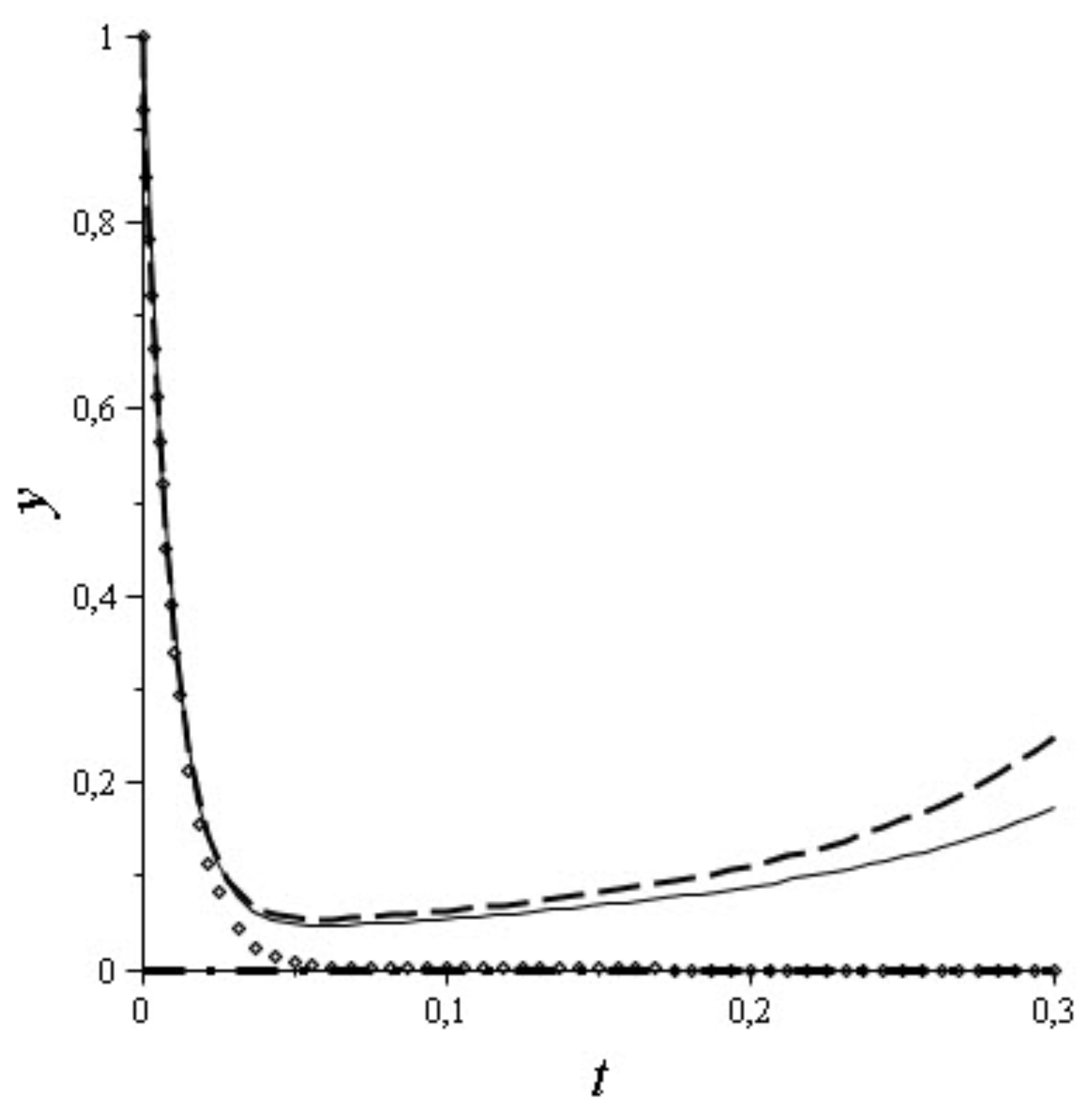
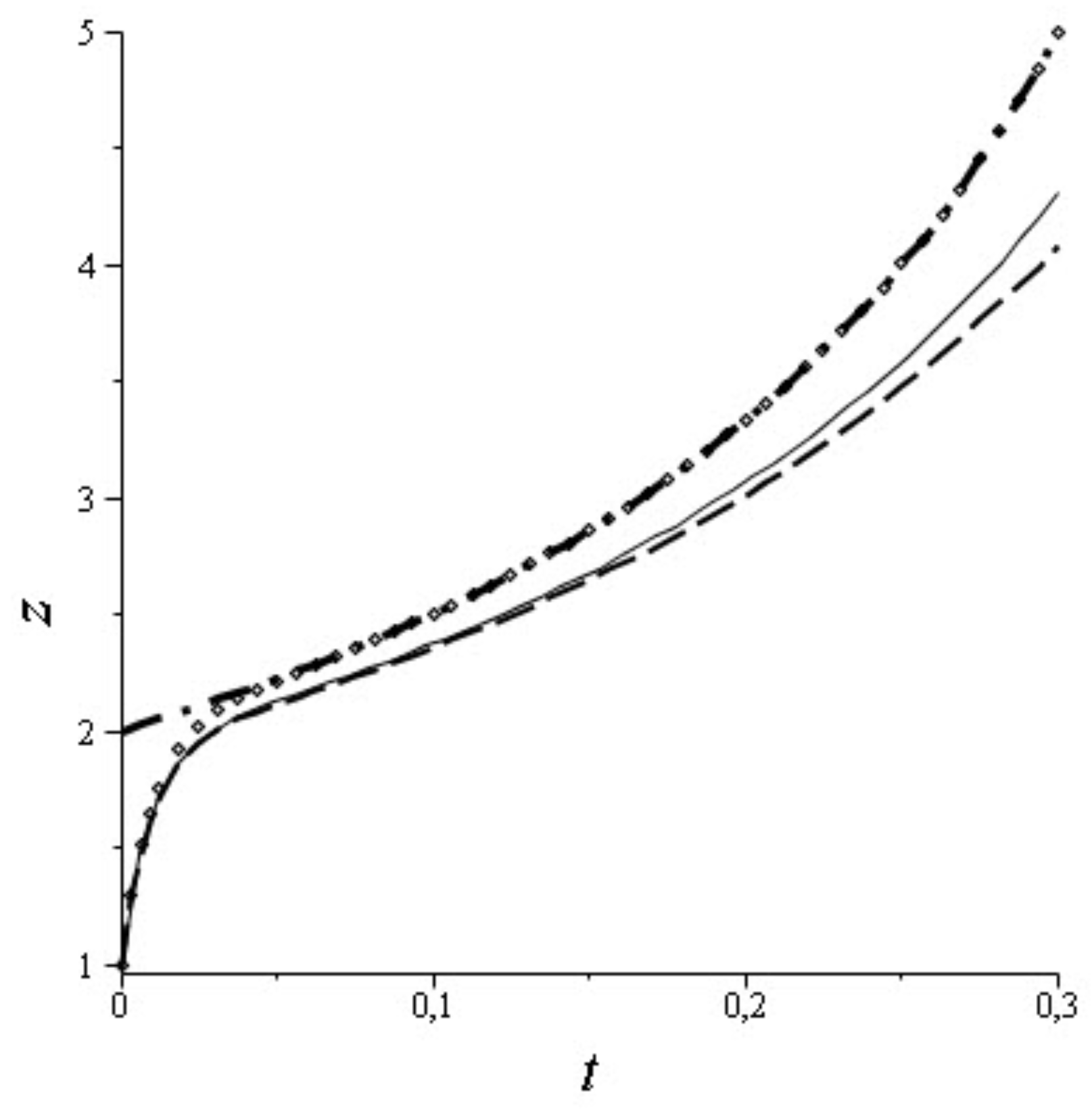
Of course, these results can be obtained using the algorithm from [4], but we would like to demonstrate here the use of projectors for finding asymptotics terms. The results obtained by Maple 13 are given in Figure 1 and Figure 2. They have been presented for the completeness of the paper. The solid line represents the exact solution; the dash-dotted line—the solution of the degenerate problem, the line consisting of squares represents the zero-order approximation; and the dash line represents the the first-order approximation. These graphs show that an asymptotic solution is closer to the exact one if we use higher-order asymptotics. If we use the smaller value of $\epsilon$, then it will result in an asymptotic solution more similar to the exact one. The graphs of the solution of the degenerate problem and the zero-order approximation illustrate the known property of boundary functions that are essential only for arguments in some vicinities of points where additional conditions are prescribed.

Figure 1. Trajectory $y(t,\epsilon )$ with $\epsilon =0.01$ and its approximations.

Figure 2. Trajectory $z(t,\epsilon )$ with $\epsilon =0.01$ and its approximations.

7. Conclusions

This paper dealt with a new approach to the algorithm of the method of boundary functions from [4] for asymptotic solving initial value problem of form (1)-(2) in the critical case. Namely, the algorithm was formulated with the help of orthogonal projectors of the space X onto $kerA\left(t\right)$ and $kerA{\left(t\right)}^{\prime }$. Such an approach clearly shows the structure of the algorithm for finding asymptotics terms, given in Table 1 and Table 2 of the paper.