Correlated Mean–Precision Random-Effects Beta Regression for Clustered Proportion Data

Abstract

Clustered proportion responses often exhibit bounded support, skewness, heterogeneous dispersion, and within-cluster dependence. We propose a correlated mean–precision random-effects beta regression model that jointly represents cluster-level heterogeneity in the conditional mean and conditional precision. Its main innovation is to treat the cross-submodel random-effect correlation as a scientific estimand. The same frequentist Beta mixed model estimates and tests this correlation while allowing nonlinear adjustment and cluster-level interpretation. Penalized B-splines allow nonlinear effects in both submodels, and estimation is performed by maximizing a Laplace-approximated penalized marginal likelihood. The fitted model provides likelihood-based inference for the mean–stability association and empirical Bayes estimates for cluster ranking and quadrant classification. Among M1–M5, M5 gives the lowest average errors for conditional-mean and conditional-precision recovery and the best average AIC, cluster-level BIC, and full-data NLPD across the Monte Carlo settings considered. It is also the only model compared here that estimates and tests the latent association while retaining paired cluster effects for interpretation. All M5 fits succeeded in the enlarged 30-replication stress suite, and the five aggregate mean M5–M4 criteria favored M5 across 299 successful pairs; quadrature checks indicate where safeguards are needed under weak information. In both CDC PLACES and the representative World Bank panel of 128 eligible countries, M5 has the largest marginal likelihood, the smallest AIC and cluster-level BIC, a significant M4–M5 likelihood-ratio test, and the lowest application-specific point-prediction errors. For the World Bank data, $\widehat{\rho }=-0.500$ (profile 95% interval $-0.621$ to $-0.295$), the likelihood-ratio statistic is $17.370$ ($p=3.08\times {10}^{-5}$), and M5 has the lowest rolling-origin MSPE, RMSE, and MAE. On the combined evidence from fit, prediction, and correlation inference, M5 is the best overall model evaluated in both applications.

1. Introduction

Proportion responses are frequently encountered in empirical research, including biomedical rates, ecological coverage, educational achievement shares, regional economic proportions, financial ratios, and other bounded outcomes. Such responses are naturally constrained to the unit interval and often display skewness, heteroscedasticity, and non-Gaussian distributional shapes. When the response satisfies $0<Y<1$, direct use of ordinary Gaussian regression may be inappropriate because it ignores the bounded support and may lead to fitted values outside the admissible range. Beta regression provides a natural likelihood-based framework for continuous proportion data because the Beta distribution is supported on $(0,1)$ and can flexibly accommodate asymmetric and heteroscedastic response patterns [1,2,3].

A key advantage of Beta regression is the mean–precision parameterization. Under this parameterization, the conditional distribution is written as $Y\sim \mathrm{Beta}(\mu \varphi ,(1-\mu \left)\varphi \right)$, where $\mu$ represents the conditional mean and $\varphi$ represents the conditional precision. The parameter $\mu$ describes the average proportion level, whereas $\varphi$ controls the concentration of the response around the mean. A larger value of $\varphi$ corresponds to a smaller conditional variance and hence a more stable response in the conditional distributional sense. Therefore, Beta regression is not only a model for the conditional mean but also a distributional model that can describe the reliability or concentration of proportion responses through the precision component. This distinction is important in applications where the scientific question concerns both the magnitude and the variability of a proportion response [2,4,5].

Many practical proportion datasets are clustered or longitudinal. Observations may be grouped by subjects, hospitals, schools, regions, firms, states, or other higher-level units. In such data, observations from the same cluster are usually more similar than observations from different clusters because they share unobserved characteristics. Ignoring this dependence may underestimate uncertainty and obscure important between-cluster heterogeneity. Random-effects models and generalized linear mixed models are commonly used to account for clustered data structures [6,7,8]. For proportion responses, random effects may enter the mean submodel to describe cluster-specific deviations in average levels. However, between-cluster heterogeneity may also appear in the precision submodel. Two clusters may have similar conditional means but very different levels of conditional concentration. Conversely, one cluster may have a high average proportion but unstable responses, whereas another may have a lower average proportion but much more concentrated responses. This phenomenon cannot be fully characterized by a mean-only random-effects model [6,7,8].

Existing Beta regression-type models have developed in several directions. Classical Beta regression focuses primarily on the conditional mean, with either constant or varying precision [1,2,4]. Distributional regression and generalized additive models for location, scale, and shape allow covariates to affect more than one distributional parameter [9,10,11]. Semiparametric extensions further introduce smooth effects to capture nonlinear covariate relationships, often through splines or penalized splines [12,13,14]. Mixed Beta regression models introduce random effects for clustered or longitudinal proportion data [15,16,17]. These developments provide important tools for bounded responses, but the direct association between cluster-specific mean heterogeneity and cluster-specific precision heterogeneity has received comparatively less focused treatment [18,19,20].

The proposed model jointly specifies semiparametric predictors for the mean and precision, paired cluster-level random effects, and an estimated cross-submodel correlation. We treat this correlation as a scientific quantity in its own right, rather than as an ancillary covariance term, and link it to likelihood-based inference and cluster-level interpretation.

This formulation estimates both sources of cluster heterogeneity together with their covariance. It also distinguishes the correlated model from its nested independence model and converts the fitted association into interpretable cluster summaries. Penalized B-splines adjust for nonlinear effects in both submodels.

Frequentist inference is based on the M4–M5 likelihood-ratio comparison and confidence intervals for $\rho$ constructed on a transformed scale. Empirical Bayes estimates of the paired random effects are used for prediction, ranking, and mean–stability quadrant classification. A Laplace-approximated penalized marginal likelihood supplies a tractable likelihood target for estimation and testing [21].

The resulting model extends mean-focused cluster adjustment to joint inference on mean heterogeneity, precision heterogeneity, and their dependence. It can therefore address whether clusters with higher adjusted average levels tend to be more or less stable, a question that ordinary mean regression, independent mean–precision random-effects models, and point-prediction methods do not answer [22].

The association between mean level and stability is scientifically meaningful. In a regional study, it may be important to know whether regions with larger average shares are also more stable in the conditional distributional sense. In a biomedical study, one may ask whether subjects with higher average response rates have more concentrated or more dispersed outcomes. In an educational or institutional study, groups with high average performance may not necessarily be the most stable groups. These questions cannot be answered by marginal mean regression alone. They require a model that simultaneously contains cluster-level heterogeneity in the mean and precision submodels and explicitly quantifies the dependence between the two latent components. This motivates the correlated mean–precision random-effects Beta regression model proposed in this paper [23,24].

Motivated by this distinction, the proposed model uses a logit link for the conditional mean and a log link for the conditional precision. Cluster-specific random effects are introduced into both submodels. Let $b_i$ denote the mean random effect and $c_i$ denote the precision random effect for cluster i. The central modeling assumption is that ${(b_i,c_i)}^{\top }$ follows a bivariate normal distribution with covariance matrix containing the correlation parameter $\rho$. The parameter $\rho =\mathrm{Corr}(b_i,c_i)$ is the primary inferential target. If $\rho >0$, clusters with higher latent mean levels tend to have higher latent precision, meaning that higher-average clusters are also more concentrated around their conditional means. If $\rho <0$, clusters with higher latent mean levels tend to have lower precision, meaning that higher-average clusters are more variable. If $\rho =0$, the latent mean heterogeneity and latent precision heterogeneity are uncorrelated after adjusting for observed covariates and smooth effects [6,23]. This interpretation is conditional on the observed covariates, the smooth effects, and the assumed bivariate random-effects structure.

Recent computational work has used a radial-basis-function neural network to solve a diffusion partial differential equation and an RBF–FD method to price options under stochastic volatility and jump processes [25,26]. Although these studies address differential equations rather than clustered regression, each adapts its basis construction to the numerical problem at hand.

The proposed model also incorporates semiparametric smooth effects in both distributional components. Specifically, unknown smooth functions are represented by penalized B-splines. This allows nonlinear covariate effects to be captured without sacrificing the interpretability of the mean and precision submodels. Centering constraints are imposed on the smooth components to avoid confounding with intercepts. Roughness penalties are used to regularize the spline coefficients. Thus, the model combines three elements in a single likelihood-based framework: Beta mean–precision modeling, bivariate cluster-level random effects, and semiparametric nonlinear effects [12,13].

Estimation is carried out by maximizing a penalized marginal likelihood. Because the random effects are latent, the likelihood involves cluster-level integration. The bivariate integral generally has no closed-form solution due to the nonlinear Beta likelihood. We therefore use a Laplace approximation to obtain a computationally tractable marginal likelihood. For each cluster, the posterior mode of the random effect is computed and the local curvature is used to approximate the integral. The resulting Laplace-approximated penalized marginal likelihood is then optimized over the fixed effects, spline coefficients, variance components, and correlation parameter. To handle parameter constraints, the standard deviations are transformed by logarithms and the correlation parameter is transformed through $\rho =\tanh \left(\xi \right)$. This guarantees positive variance components and $-1<\rho <1$ during numerical optimization [7,27].

Under the fitted model, the proposed framework provides several inferential and exploratory diagnostic outputs. First, it yields estimates of fixed effects and nonlinear smooth components in both the mean and precision submodels. Second, it provides estimates of the between-cluster mean heterogeneity, between-cluster precision heterogeneity, and their correlation. Third, it supports formal testing of the mean–stability association through Wald-type or likelihood-ratio procedures for $H_0:\rho =0$. Fourth, it produces empirical Bayes estimates of the cluster-level random effects. These estimates can be used to rank clusters by adjusted mean level and adjusted stability. They also support exploratory mean–stability quadrant diagnosis, separating clusters into high mean–high stability, high mean–low stability, low mean–high stability, and low mean–low stability groups [8,28]. This diagnostic summary is not intended to replace full uncertainty quantification, but it provides an interpretable cluster-level view that cannot be obtained from ordinary mean regression or black-box point-prediction methods. In the numerical studies, the likelihood-ratio test is used as the primary inferential tool for $\rho$.

This paper develops a frequentist model for clustered continuous proportions. M5 jointly represents heterogeneity in the conditional mean and precision and uses $\rho$ to quantify their latent association. Estimation uses a Laplace-approximated penalized marginal likelihood with centered penalized B-splines in both submodels. Confidence intervals on a transformed scale and the nested M4–M5 likelihood-ratio comparison provide inference for $\rho$; paired empirical Bayes effects support cluster ranking and mean–stability quadrant diagnosis. We examine the model in Monte Carlo experiments and in two different domains: CDC PLACES county-level short-sleep prevalence and a World Bank country-year panel of renewable-energy consumption shares.

Table 1. Comparison of established approaches for clustered continuous proportions. The final column records the features that distinguish M5, including direct frequentist inference for $\rho$ and a paired mean–stability interpretation.

Framework	Mean and Precision Predictors	Paired Group Effects	Cross-Submodel Correlation	Primary Inferential Paradigm	Relation to the Proposed Innovation
Mean-only Beta mixed model	Mean only	No	No	Frequentist or Bayesian	Models clustered means but cannot recover cluster-specific precision heterogeneity or mean–stability dependence.
GAMLSS/structured distributional regression	Yes	Implementation-dependent	Possible	Frequentist or Bayesian	Offers broad distributional flexibility, whereas M5 supplies a dedicated $\rho$-centered likelihood test and paired cluster interpretation.
Generalized additive mixed model	Usually one response parameter	Model-dependent	Model-dependent	Usually frequentist	Provides smooth mixed modeling, whereas M5 jointly targets mean heterogeneity, precision heterogeneity, and their association.
Bayesian hierarchical Beta regression	Yes	Yes	Yes	Posterior inference	Provides posterior inference; M5 contributes a direct frequentist marginal likelihood route with a nested independence test and transformed-scale interval.
Independent mean–precision effects (M4)	Yes	Yes	Fixed at zero	Frequentist marginal likelihood	Is the nested comparator that M5 extends by estimating, testing, and interpreting cross-submodel dependence.
Proposed correlated model (M5)	Yes	Yes	Estimated as $\rho$	Frequentist penalized marginal likelihood	Combines nonlinear adjustment, correlated paired effects, formal $\rho$ inference, prediction, and empirical Bayes mean–stability diagnosis.

compares the proposed model with commonly used alternatives. M5 is the only approach in the table that combines semiparametric mean and precision predictors, paired correlated cluster effects, direct frequentist inference for $\rho$, a nested independence test, and an empirical Bayes interpretation of mean and stability. Its distinguishing feature is that cluster-level dependence between the two submodels is estimated, tested, and interpreted. The comparison draws on recent SCI studies of distributional regression, hierarchical Beta models, likelihood-based GLMM inference, and multivariate distributional modeling [8,10,16,29,30].

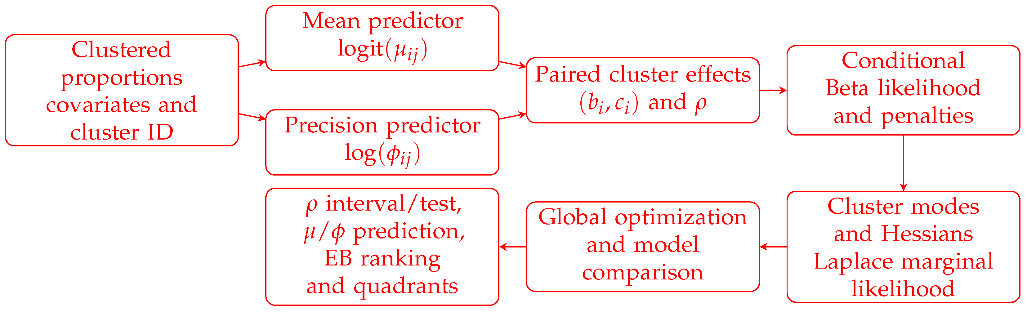
Figure 1 separates the statistical workflow from the numerical details in Algorithm 1.

Monte Carlo simulations examine finite-sample performance across different correlations, sample sizes, variance settings, nonlinear functions, and boundary cases. Among M1–M5, M5 has the lowest average recovery errors for the conditional mean and precision and the best average AIC, cluster-level BIC, and full-data NLPD across the 23 settings. The enlarged stress suite uses 30 replications in each of ten nonnull settings; every M5 fit succeeds, and all five aggregate mean M5–M4 criteria favor M5 across 299 successful pairs. The M4–M5 likelihood-ratio test controls type I error when $\rho =0$ and has high power under strong positive or negative latent correlations. For new clusters, M5 matches the point-prediction accuracy of the leading competitors and, unlike them, recovers and tests the latent correlation while retaining the paired effects needed for mean–stability interpretation [4].

A real-data analysis of the CDC PLACES county-level dataset is used to illustrate the practical value of the proposed framework. The observational unit is a county, and counties are clustered by state. The response is the county-level adjusted prevalence proportion for short sleep duration, constructed as SLEEP-AdjPrev/100. The fitted results are used to assess whether state-level heterogeneity appears only in the mean component or also in the precision component, and whether the two latent state-level components are associated under the fitted model [31].

The second application tests the model outside public health using the World Bank World Development Indicators country-year panel. The response is the observed share of renewable energy in total final energy consumption, countries are the clusters, and covariates describing development, industry, urbanization, and energy systems enter the mean and precision submodels. The main analysis includes all 128 countries that meet the prespecified completeness and open-interval rules and fits the same M1–M5 hierarchy. Model-consistent residual and influence diagnostics are reported. Prediction to unseen countries is assessed by repeated grouped cross-validation in a fixed balanced sample of 24 countries, and prediction of future years for observed countries is assessed at three rolling origins.

Section 2 defines the correlated mean–precision random-effects Beta regression model, its semiparametric components, identifiability conditions, and nested special cases. Section 3 describes estimation, inference for $\rho$, model comparison, prediction, and cluster-level interpretation. Section 4 and Section 5 report the Monte Carlo experiments and the two real-data applications, respectively. Section 6 summarizes the findings, limitations, and possible extensions.

2. Methodology

2.1. Model Setting

Let $Y_{ij}$ denote the proportion response observed from the j-th unit in the i-th cluster, where $i=1,\dots ,m$ and $j=1,\dots ,n_i$. The total sample size is $N={\sum }_{i=1}^m{n}_i$. Throughout this paper, we consider continuous proportion responses satisfying $0<Y_{ij}<1$. Such data naturally arise in longitudinal, regional, biomedical, ecological, educational, and economic studies, where observations are grouped by subjects, regions, schools, hospitals, firms, or other cluster-level units. The cluster structure is important because observations from the same cluster may share unobserved characteristics that simultaneously affect the average proportion level and the stability of the observed proportions. For each observation, let $x_{ij}\in {\mathbb{R}}^p$ be a vector of covariates associated with the conditional mean of $Y_{ij}$, and let $z_{ij}\in {\mathbb{R}}^q$ be a vector of covariates associated with the conditional precision of $Y_{ij}$. Unless otherwise stated, the first components of $x_{ij}$ and $z_{ij}$ are set to one, so that both the mean and precision submodels contain intercept terms. The two covariate vectors may be identical, partially overlapping, or completely different. In addition, let $w_{ij}$ and $s_{ij}$ denote scalar or low-dimensional covariates whose effects on the mean and precision components are allowed to be nonlinear. The proposed model is designed to answer three related questions: whether the average proportion differs across clusters, whether the stability of the proportion differs across clusters, and whether the cluster-specific average level and cluster-specific stability are associated. The Beta distribution is adopted for the response variable. Conditional on the cluster-level random effects and observed covariates, observations within the same cluster are assumed to be independent. Therefore, the within-cluster dependence is induced by the shared random effects. Conditional on the mean parameter ${\mu }_{ij}$ and the precision parameter ${\varphi }_{ij}$, we assume

$$Y_{ij}\mid {\mu }_{ij},{\varphi }_{ij}\sim \mathrm{Beta}\left({\mu }_{ij}{\varphi }_{ij},(1-{\mu }_{ij}){\varphi }_{ij}\right),$$

(1)

where $0<{\mu }_{ij}<1$ and ${\varphi }_{ij}>0$. Under this mean–precision parameterization,

$$E(Y_{ij}\mid {\mu }_{ij},{\varphi }_{ij})={\mu }_{ij},$$

(2)

and

$$\mathrm{Var}(Y_{ij}\mid {\mu }_{ij},{\varphi }_{ij})={\displaystyle \frac{{\mu }_{ij}(1-{\mu }_{ij})}{1+{\varphi }_{ij}}}.$$

(3)

Thus, ${\mu }_{ij}$ controls the conditional average proportion, whereas ${\varphi }_{ij}$ controls the conditional concentration of the response around its mean. In this paper, stability is used in a conditional distributional sense: after adjusting for covariates and cluster-level effects, a larger precision parameter implies a smaller conditional variance and hence a more stable proportion response. For notational convenience, define the two shape parameters

$$A_{ij}={\mu }_{ij}{\varphi }_{ij},Q_{ij}=(1-{\mu }_{ij}){\varphi }_{ij}.$$

(4)

The conditional density of $Y_{ij}$ is

$$f(y_{ij}\mid {\mu }_{ij},{\varphi }_{ij})={\displaystyle \frac{\mathrm{\Gamma }\left({\varphi }_{ij}\right)}{\mathrm{\Gamma }\left({\mu }_{ij}{\varphi }_{ij}\right)\mathrm{\Gamma }\left((1-{\mu }_{ij}){\varphi }_{ij}\right)}}{y}_{ij}^{{\mu }_{ij}{\varphi }_{ij}-1}{(1-y_{ij})}^{(1-{\mu }_{ij}){\varphi }_{ij}-1}.$$

(5)

The corresponding conditional log-density is

$$\begin{array}{cc}\hfill {\mathsf{\ell }}_{ij}=& \log \mathrm{\Gamma }\left({\varphi }_{ij}\right)-\log \mathrm{\Gamma }\left({\mu }_{ij}{\varphi }_{ij}\right)-\log \mathrm{\Gamma }\left((1-{\mu }_{ij}){\varphi }_{ij}\right)\hfill \\ \hfill & +({\mu }_{ij}{\varphi }_{ij}-1)\log y_{ij}+((1-{\mu }_{ij}){\varphi }_{ij}-1)\log (1-y_{ij}).\hfill \end{array}$$

(6)

The proposed model contains two distributional submodels. The conditional mean is modeled by

$$\mathrm{logit}\left({\mu }_{ij}\right)=x_{ij}^{\top }\beta +f\left(w_{ij}\right)+b_i,$$

(7)

where $\beta \in {\mathbb{R}}^p$ is the fixed-effect coefficient vector in the mean submodel, $f(·)$ is an unknown smooth function, and $b_i$ is a cluster-specific random effect acting on the mean component. The random effect $b_i$ represents the latent deviation of cluster i from the population-level mean structure after adjusting for the observed covariates and the smooth effect. The conditional precision is modeled by

$$\log \left({\varphi }_{ij}\right)=z_{ij}^{\top }\gamma +g\left(s_{ij}\right)+c_i,$$

(8)

where $\gamma \in {\mathbb{R}}^q$ is the fixed-effect coefficient vector in the precision submodel, $g(·)$ is an unknown smooth function, and $c_i$ is a cluster-specific random effect acting on the precision component. Since the precision parameter is inversely related to the conditional variance, $c_i$ can be interpreted as a latent stability effect of cluster i. Define the two linear predictors by

$${\eta }_{ij}^{\mu }=x_{ij}^{\top }\beta +f\left(w_{ij}\right)+b_i,$$

(9)

and

$${\eta }_{ij}^{\varphi }=z_{ij}^{\top }\gamma +g\left(s_{ij}\right)+c_i.$$

(10)

Then,

$${\mu }_{ij}={\displaystyle \frac{\exp \left({\eta }_{ij}^{\mu }\right)}{1+\exp \left({\eta }_{ij}^{\mu }\right)}},$$

(11)

and

$${\varphi }_{ij}=\exp \left({\eta }_{ij}^{\varphi }\right).$$

(12)

The two submodels have distinct interpretations. The coefficient vector $\beta$ and the smooth function $f(·)$ explain systematic changes in the average proportion, whereas $\gamma$ and $g(·)$ explain systematic changes in the response stability. A covariate may affect the conditional mean, the conditional precision, or both. The central component of the proposed model is the joint distribution of $b_i$ and $c_i$. We assume that the cluster-level mean random effect and the cluster-level precision random effect follow a bivariate normal distribution:

$$\left(\begin{array}{c}{b}_i\\ c_i\end{array}\right)\sim N_2\left[\left(\begin{array}{c}0\\ 0\end{array}\right),\mathrm{\Sigma }\right],$$

(13)

where

$$\mathrm{\Sigma }=\left(\begin{array}{cc}{\sigma }_b^2& \rho {\sigma }_b{\sigma }_c\\ \rho {\sigma }_b{\sigma }_c& {\sigma }_c^2\end{array}\right),{\sigma }_b>0,{\sigma }_c>0,-1<\rho <1.$$

(14)

Here, ${\sigma }_b^2$ measures the magnitude of between-cluster heterogeneity in the mean component, while ${\sigma }_c^2$ measures the magnitude of between-cluster heterogeneity in the precision component [6,15,23]. The parameter

$$\rho =\mathrm{Corr}(b_i,c_i)$$

(15)

is the main inferential target of the proposed model. The interpretation of $\rho$ is meaningful when both variance components are positive. If either ${\sigma }_b^2$ or ${\sigma }_c^2$ is zero, the corresponding random effect degenerates and the correlation parameter is not identifiable. If $\rho >0$, clusters with higher latent mean levels tend to have higher latent precision levels. In this case, groups with higher average proportions are also more stable. If $\rho <0$, clusters with higher latent mean levels tend to have lower latent precision levels, meaning that groups with higher average proportions are more variable. If $\rho =0$, the latent mean heterogeneity and latent precision heterogeneity are uncorrelated after adjusting for observed covariates. The covariance matrix in (14) has determinant

$$\left|\mathrm{\Sigma }\right|={\sigma }_b^2{\sigma }_c^2(1-{\rho }^2),$$

(16)

and inverse

$${\mathrm{\Sigma }}^{-1}={\displaystyle \frac{1}{1-{\rho }^2}}\left(\begin{array}{cc}{\sigma }_b^{-2}& -\rho {\left({\sigma }_b{\sigma }_c\right)}^{-1}\\ -\rho {\left({\sigma }_b{\sigma }_c\right)}^{-1}& {\sigma }_c^{-2}\end{array}\right).$$

(17)

To allow nonlinear effects while preserving interpretability, the unknown functions $f(·)$ and $g(·)$ are represented by penalized B-splines [12,13]. Let $B_1(·),\dots ,B_{K_f}(·)$ be B-spline basis functions for the mean submodel and $C_1(·),\dots ,C_{K_g}(·)$ be B-spline basis functions for the precision submodel. We write

$$f\left(w\right)={\displaystyle \sum _{k=1}^{K_f}}{\alpha }_k{B}_k\left(w\right)=B{\left(w\right)}^{\top }\alpha ,$$

(18)

and

$$g\left(s\right)={\displaystyle \sum _{l=1}^{K_g}}{\delta }_l{C}_l\left(s\right)=C{\left(s\right)}^{\top }\delta ,$$

(19)

where $B\left(w\right)={(B_1\left(w\right),\dots ,B_{K_f}\left(w\right))}^{\top }$, $C\left(s\right)={(C_1\left(s\right),\dots ,C_{K_g}\left(s\right))}^{\top }$, $\alpha ={({\alpha }_1,\dots ,{\alpha }_{K_f})}^{\top }$, and $\delta ={({\delta }_1,\dots ,{\delta }_{K_g})}^{\top }$. To avoid confounding between intercepts and smooth components, the spline bases are centered in implementation. Equivalently, the smooth functions satisfy the empirical centering constraints

$${\displaystyle \sum _{i=1}^m}{\displaystyle \sum _{j=1}^{n_i}}f\left(w_{ij}\right)=0,{\displaystyle \sum _{i=1}^m}{\displaystyle \sum _{j=1}^{n_i}}g\left(s_{ij}\right)=0.$$

(20)

Let $D_f$ and $D_g$ denote difference matrices for the mean and precision smooth terms. The roughness penalties are

$$P_f\left(\alpha \right)={\displaystyle \frac{{\lambda }_f}{2}}{\alpha }^{\top }{D}_f^{\top }{D}_f\alpha ,$$

(21)

and

$$P_g\left(\delta \right)={\displaystyle \frac{{\lambda }_g}{2}}{\delta }^{\top }{D}_g^{\top }{D}_g\delta ,$$

(22)

where ${\lambda }_f\ge 0$ and ${\lambda }_g\ge 0$ are smoothing parameters. The smooth components improve model flexibility, but the primary inferential target remains the correlation parameter $\rho$. Substituting (18) and (19) into (7) and (8), the semiparametric predictors are

$${\eta }_{ij}^{\mu }=x_{ij}^{\top }\beta +B{\left(w_{ij}\right)}^{\top }\alpha +b_i,$$

(23)

and

$${\eta }_{ij}^{\varphi }=z_{ij}^{\top }\gamma +C{\left(s_{ij}\right)}^{\top }\delta +c_i.$$

(24)

Definition 1.

The model defined by (1), (23), (24), and (13) is called the correlated mean–precision random-effects Beta regression model. It is a distributional random-effects model because random effects are introduced into both the mean and precision submodels, and the association between the two latent cluster-level components is explicitly quantified by ρ. The sign of ρ has a conditional, model-scale interpretation. If $\rho >0$, clusters above the fitted population mean on the logit scale tend also to have higher conditional precision. If $\rho <0$, clusters above the fitted mean tend to have lower precision and hence greater conditional dispersion. If $\rho \approx 0$, the two adjusted latent deviations have little linear association. These statements concern the random effects after adjustment for the specified covariates and smooth terms. They are not causal statements, and the practical magnitude depends jointly on ρ, ${\sigma }_b$, ${\sigma }_c$, and the two link functions. In particular,

$$E(c_i\mid b_i)=\rho {\displaystyle \frac{{\sigma }_c}{{\sigma }_b}}{b}_i,\mathrm{Cov}(b_i,c_i)=\rho {\sigma }_b{\sigma }_c.$$

(25)

Thus, the same numerical correlation can imply different changes in precision when the variance components differ.

2.2. Identifiability and Special Cases

For the full correlated random-effects model to be identifiable, the following conditions are assumed.

Assumption 1.

The fixed-effect design matrices in the mean and precision submodels have full column rank after accounting for intercept terms and centered spline bases. The smooth components are centered as in (20). The random effects have zero means. The covariance matrix Σ is positive definite, namely ${\sigma }_b>0$, ${\sigma }_c>0$, and $-1<\rho <1$. The response values lie in the open unit interval, namely $0<Y_{ij}<1$.

Under Assumption 1, the population-level intercepts, smooth components, and cluster-level deviations are separated. The fixed effects and smooth terms in the mean submodel determine the population-level average proportion, whereas the fixed effects and smooth terms in the precision submodel determine the population-level stability. The random effect $b_i$ measures how much cluster i deviates from the population-level mean structure, while $c_i$ measures how much cluster i deviates from the population-level stability structure. The correlation $\rho$ summarizes whether these two latent cluster characteristics tend to move together.

Remark 1

(weak identification of $\rho$). The covariance sensitivity to the correlation parameter is

$${\displaystyle \frac{\partial \mathrm{\Sigma }}{\partial \rho }}={\sigma }_b{\sigma }_c\left(\begin{array}{cc}0& 1\\ 1& 0\end{array}\right).$$

(26)

Consequently, the marginal likelihood becomes progressively less sensitive to ρ as either standard deviation approaches zero. The number of independent clusters m, rather than only the total observation count, supplies the main replication for estimating a between-cluster correlation. Larger $n_i$ improves estimation of each cluster’s paired effects, but it cannot replace an adequate number of clusters. Strong imbalance can further concentrate information in a small number of large clusters. If either variance is exactly zero, ρ is undefined and the corresponding reduced model should be fitted. Near a boundary, a flat profile likelihood, a poorly conditioned observed information matrix, or a confidence interval spanning most of $(-1,1)$ should be reported as weak-identification warnings rather than interpreted as precise evidence about association.

Assumption 1 is imposed for the full correlated random-effects model. Some reduced models discussed below are obtained by placing variance components on the boundary of the parameter space [16,17,32]. These reduced models are used for interpretation, model comparison, and sensitivity analysis [33,34]. The proposed model contains several important models as special cases. If ${\sigma }_b^2={\sigma }_c^2=0$, the random effects vanish and the model reduces to a semiparametric varying-precision Beta regression:

$$\mathrm{logit}\left({\mu }_{ij}\right)=x_{ij}^{\top }\beta +f\left(w_{ij}\right),\log \left({\varphi }_{ij}\right)=z_{ij}^{\top }\gamma +g\left(s_{ij}\right).$$

(27)

If ${\varphi }_{ij}=\varphi$ is constant and ${\sigma }_b^2={\sigma }_c^2=0$, the model reduces to a semiparametric constant-precision Beta regression:

$$Y_{ij}\sim \mathrm{Beta}({\mu }_{ij}\varphi ,(1-{\mu }_{ij})\varphi ),\mathrm{logit}\left({\mu }_{ij}\right)=x_{ij}^{\top }\beta +f\left(w_{ij}\right).$$

(28)

If, in addition, $f(·)=0$, the model becomes the classical Beta regression model with constant precision:

$$Y_{ij}\sim \mathrm{Beta}({\mu }_{ij}\varphi ,(1-{\mu }_{ij})\varphi ),\mathrm{logit}\left({\mu }_{ij}\right)=x_{ij}^{\top }\beta .$$

(29)

If $\rho =0$, the two random effects are independent:

$$b_i\perp c_i.$$

(30)

This independent mean–precision random-effects model still allows separate cluster heterogeneity in the mean and precision components, but it does not allow the two latent heterogeneities to be associated. It is therefore the most important competing model for testing the necessity of the proposed correlated random-effects structure. If ${\sigma }_c^2=0$, the precision random effect is absent and the model reduces to a Beta mixed model with a random effect only in the mean submodel. If ${\sigma }_b^2=0$, the model contains a random effect only in the precision submodel.

Proposition 1.

The classical constant-precision Beta regression model, the varying-precision Beta regression model, the mean-only random-effects Beta model, and the independent mean–precision random-effects Beta model are nested special cases of the proposed correlated mean–precision random-effects Beta regression model.

Proof. 

The result follows directly from the restrictions ${\sigma }_b^2={\sigma }_c^2=0$, ${\varphi }_{ij}=\varphi$, $f(·)=0$, ${\sigma }_c^2=0$, and $\rho =0$, respectively. These restrictions reduce the proposed model to the corresponding submodels described above.    □

The proposed model has three main features. First, it models the conditional mean and conditional precision simultaneously. Second, it allows both components to contain cluster-level heterogeneity. Third, it directly quantifies the latent association between group-specific mean level and group-specific stability through the correlation parameter $\rho$.

3. Parameter Estimation and Inference

3.1. Penalized Marginal Likelihood and Laplace Approximation

The estimation problem is challenging because the likelihood involves integration over bivariate random effects and because the smooth components require regularization. We therefore construct a penalized marginal likelihood and approximate the cluster-level integrals using the Laplace approximation [7,27]. Let $r_i={(b_i,c_i)}^{\top }$ denote the bivariate random effect for cluster i. Let

$$\theta ={({\beta }^{\top },{\gamma }^{\top },{\alpha }^{\top },{\delta }^{\top },{\sigma }_b,{\sigma }_c,\rho )}^{\top }$$

(31)

collect the finite-dimensional model parameters. The smoothing parameters ${\lambda }_f$ and ${\lambda }_g$ are treated as tuning parameters selected by information criteria or cross-validation and are therefore not included in $\theta$. Conditional on $r_i$, observations within cluster i are assumed to be independent. The conditional log-likelihood contribution of cluster i is

$${\mathsf{\ell }}_i(\theta ;r_i)={\displaystyle \sum _{j=1}^{n_i}}{\mathsf{\ell }}_{ij}(\theta ;r_i),$$

(32)

where ${\mathsf{\ell }}_{ij}$ is given in (6), with ${\mu }_{ij}$ and ${\varphi }_{ij}$ determined by (23) and (24). The complete-data log-likelihood, treating the random effects as latent variables, is

$${\mathsf{\ell }}_c(\theta ;R)={\displaystyle \sum _{i=1}^m}\left\{{\mathsf{\ell }}_i(\theta ;r_i)+\log {\phi }_2(r_i;0,\mathrm{\Sigma })\right\},$$

(33)

where $R={(r_1^{\top },\dots ,r_m^{\top })}^{\top }$ and ${\phi }_2(·;0,\mathrm{\Sigma })$ denotes the bivariate normal density with mean zero and covariance matrix $\mathrm{\Sigma }$. Using (16) and (17), the log-density of $r_i$ is

$$\log {\phi }_2(r_i;0,\mathrm{\Sigma })=-\log \left(2\pi \right)-{\displaystyle \frac{1}{2}}\log \left|\mathrm{\Sigma }\right|-{\displaystyle \frac{1}{2}}{r}_i^{\top }{\mathrm{\Sigma }}^{-1}{r}_i.$$

(34)

Substituting (34) into (33), we obtain

$${\mathsf{\ell }}_c(\theta ;R)={\displaystyle \sum _{i=1}^m}{\displaystyle \sum _{j=1}^{n_i}}{\mathsf{\ell }}_{ij}(\theta ;r_i)-{\displaystyle \frac{m}{2}}\log \left|\mathrm{\Sigma }\right|-{\displaystyle \frac{1}{2}}{\displaystyle \sum _{i=1}^m}{r}_i^{\top }{\mathrm{\Sigma }}^{-1}{r}_i-m\log \left(2\pi \right).$$

(35)

Since $r_i$ is unobserved, inference is based on the marginal likelihood obtained by integrating out the random effects. The marginal likelihood contribution of cluster i is

$$L_i\left(\theta \right)={\int }_{{\mathbb{R}}^2}\exp \left\{{\mathsf{\ell }}_i(\theta ;r_i)\right\}{\phi }_2(r_i;0,\mathrm{\Sigma })d{r}_i.$$

(36)

Define

$$h_i(r_i;\theta )={\mathsf{\ell }}_i(\theta ;r_i)+\log {\phi }_2(r_i;0,\mathrm{\Sigma }).$$

(37)

Then, (36) can be written as

$$L_i\left(\theta \right)={\int }_{{\mathbb{R}}^2}\exp \left\{h_i(r_i;\theta )\right\}d{r}_i.$$

(38)

The full marginal log-likelihood is

$$\mathsf{\ell }\left(\theta \right)={\displaystyle \sum _{i=1}^m}\log L_i\left(\theta \right).$$

(39)

When smooth functions are included, the spline coefficients are regularized. The penalized marginal log-likelihood is

$${\mathsf{\ell }}_p\left(\theta \right)=\mathsf{\ell }\left(\theta \right)-{\displaystyle \frac{{\lambda }_f}{2}}{\alpha }^{\top }{D}_f^{\top }{D}_f\alpha -{\displaystyle \frac{{\lambda }_g}{2}}{\delta }^{\top }{D}_g^{\top }{D}_g\delta .$$

(40)

The corresponding penalized maximum likelihood estimator is

$$\widehat{\theta }=\arg \underset{\theta }{\max }{\mathsf{\ell }}_p\left(\theta \right).$$

(41)

The integral in (38) is two-dimensional but generally has no closed-form solution because the Beta likelihood is nonlinear in $b_i$ and $c_i$. For each cluster, let

$${\widehat{r}}_i\left(\theta \right)=\arg \underset{r_i\in {\mathbb{R}}^2}{\max }{h}_i(r_i;\theta )$$

(42)

be the posterior mode of the random effect under the current value of $\theta$, and let

$$H_i\left(\theta \right)=-{\left.{\displaystyle \frac{{\partial }^2{h}_i(r_i;\theta )}{\partial r_i\partial r_i^{\top }}}\right|}_{r_i={\widehat{r}}_i\left(\theta \right)}$$

(43)

be the negative Hessian matrix evaluated at the posterior mode. If $H_i\left(\theta \right)$ is positive definite, a second-order Taylor expansion of $h_i(r_i;\theta )$ around ${\widehat{r}}_i\left(\theta \right)$ gives

$$h_i(r_i;\theta )\approx h_i({\widehat{r}}_i;\theta )-{\displaystyle \frac{1}{2}}{(r_i-{\widehat{r}}_i)}^{\top }{H}_i\left(\theta \right)(r_i-{\widehat{r}}_i).$$

(44)

Substituting (44) into (38), we have

$$L_i\left(\theta \right)\approx \exp \left\{h_i({\widehat{r}}_i;\theta )\right\}{\int }_{{\mathbb{R}}^2}\exp \left\{-{\displaystyle \frac{1}{2}}{(r_i-{\widehat{r}}_i)}^{\top }{H}_i\left(\theta \right)(r_i-{\widehat{r}}_i)\right\}d{r}_i.$$

(45)

Since the random-effect dimension is two, the Gaussian integral is

$${\int }_{{\mathbb{R}}^2}\exp \left\{-{\displaystyle \frac{1}{2}}{(r_i-{\widehat{r}}_i)}^{\top }{H}_i\left(\theta \right)(r_i-{\widehat{r}}_i)\right\}d{r}_i=\left(2\pi \right){\left|H_i\left(\theta \right)\right|}^{-1/2}.$$

(46)

Thus,

$$\log L_i\left(\theta \right)\approx h_i({\widehat{r}}_i\left(\theta \right);\theta )+\log \left(2\pi \right)-{\displaystyle \frac{1}{2}}\log \left|H_i\left(\theta \right)\right|.$$

(47)

The Laplace-approximated penalized marginal log-likelihood is

$${\mathsf{\ell }}_{p,L}\left(\theta \right)={\displaystyle \sum _{i=1}^m}\left\{h_i({\widehat{r}}_i\left(\theta \right);\theta )+\log \left(2\pi \right)-{\displaystyle \frac{1}{2}}\log \left|H_i\left(\theta \right)\right|\right\}-{\displaystyle \frac{{\lambda }_f}{2}}{\alpha }^{\top }{D}_f^{\top }{D}_f\alpha -{\displaystyle \frac{{\lambda }_g}{2}}{\delta }^{\top }{D}_g^{\top }{D}_g\delta .$$

(48)

Let ${\mathsf{\ell }}_L\left(\theta \right)$ denote the unpenalized Laplace-approximated marginal log-likelihood, namely the summation term in (48) before subtracting the spline penalties. The estimator used in this paper is

$$\widehat{\theta }=\arg \underset{\theta }{\max }{\mathsf{\ell }}_{p,L}\left(\theta \right).$$

(49)

The Laplace approximation replaces the intractable marginal likelihood by a tractable objective function while preserving the cluster-level integration over the bivariate random effects. If $H_i\left(\theta \right)$ is nearly singular or not numerically positive definite, a small ridge correction can be used by replacing $H_i\left(\theta \right)$ with $H_i\left(\theta \right)+\epsilon I_2$, where $\epsilon >0$ is small [29]. For optimization, define

$$L_{ij}=\log y_{ij}-\log (1-y_{ij}).$$

(50)

Let $\psi (·)$ and ${\psi }_1(·)$ denote the digamma and trigamma functions. Differentiating (6) with respect to ${\mu }_{ij}$ and ${\varphi }_{ij}$ gives

$${\displaystyle \frac{\partial {\mathsf{\ell }}_{ij}}{\partial {\mu }_{ij}}}={\varphi }_{ij}\left\{-\psi \left(A_{ij}\right)+\psi \left(Q_{ij}\right)+L_{ij}\right\},$$

(51)

and

$${\displaystyle \frac{\partial {\mathsf{\ell }}_{ij}}{\partial {\varphi }_{ij}}}=\psi \left({\varphi }_{ij}\right)-{\mu }_{ij}\psi \left(A_{ij}\right)-(1-{\mu }_{ij})\psi \left(Q_{ij}\right)+{\mu }_{ij}\log y_{ij}+(1-{\mu }_{ij})\log (1-y_{ij}).$$

(52)

The link derivatives are

$${\displaystyle \frac{\partial {\mu }_{ij}}{\partial {\eta }_{ij}^{\mu }}}={\mu }_{ij}(1-{\mu }_{ij}),{\displaystyle \frac{\partial {\varphi }_{ij}}{\partial {\eta }_{ij}^{\varphi }}}={\varphi }_{ij}.$$

(53)

Therefore, the score contributions with respect to the two linear predictors are

$$S_{ij}^{\mu }={\displaystyle \frac{\partial {\mathsf{\ell }}_{ij}}{\partial {\eta }_{ij}^{\mu }}}={\displaystyle \frac{\partial {\mathsf{\ell }}_{ij}}{\partial {\mu }_{ij}}}{\mu }_{ij}(1-{\mu }_{ij}),$$

(54)

and

$$S_{ij}^{\varphi }={\displaystyle \frac{\partial {\mathsf{\ell }}_{ij}}{\partial {\eta }_{ij}^{\varphi }}}={\displaystyle \frac{\partial {\mathsf{\ell }}_{ij}}{\partial {\varphi }_{ij}}}{\varphi }_{ij}.$$

(55)

Consequently,

$${\displaystyle \frac{\partial {\mathsf{\ell }}_i}{\partial \beta }}={\displaystyle \sum _{j=1}^{n_i}}{S}_{ij}^{\mu }{x}_{ij},{\displaystyle \frac{\partial {\mathsf{\ell }}_i}{\partial \gamma }}={\displaystyle \sum _{j=1}^{n_i}}{S}_{ij}^{\varphi }{z}_{ij},$$

(56)

and

$${\displaystyle \frac{\partial {\mathsf{\ell }}_i}{\partial \alpha }}={\displaystyle \sum _{j=1}^{n_i}}{S}_{ij}^{\mu }B\left(w_{ij}\right),{\displaystyle \frac{\partial {\mathsf{\ell }}_i}{\partial \delta }}={\displaystyle \sum _{j=1}^{n_i}}{S}_{ij}^{\varphi }C\left(s_{ij}\right).$$

(57)

After adding the spline penalties, the penalized score components for the spline coefficients are

$${\displaystyle \frac{\partial {\mathsf{\ell }}_{p,L}}{\partial \alpha }}={\displaystyle \frac{\partial {\mathsf{\ell }}_L}{\partial \alpha }}-{\lambda }_f{D}_f^{\top }{D}_f\alpha ,{\displaystyle \frac{\partial {\mathsf{\ell }}_{p,L}}{\partial \delta }}={\displaystyle \frac{\partial {\mathsf{\ell }}_L}{\partial \delta }}-{\lambda }_g{D}_g^{\top }{D}_g\delta .$$

(58)

The negative Hessian $H_i\left(\theta \right)$ required in the Laplace approximation is computed from the second derivatives with respect to $b_i$ and $c_i$. Define

$$U_{ij}=-\psi \left(A_{ij}\right)+\psi \left(Q_{ij}\right)+L_{ij}.$$

(59)

Then

$${\displaystyle \frac{{\partial }^2{\mathsf{\ell }}_{ij}}{\partial {\mu }_{ij}^2}}=-{\varphi }_{ij}^2\left\{{\psi }_1\left(A_{ij}\right)+{\psi }_1\left(Q_{ij}\right)\right\},$$

(60)

$${\displaystyle \frac{{\partial }^2{\mathsf{\ell }}_{ij}}{\partial {\varphi }_{ij}^2}}={\psi }_1\left({\varphi }_{ij}\right)-{\mu }_{ij}^2{\psi }_1\left(A_{ij}\right)-{(1-{\mu }_{ij})}^2{\psi }_1\left(Q_{ij}\right),$$

(61)

and

$${\displaystyle \frac{{\partial }^2{\mathsf{\ell }}_{ij}}{\partial {\mu }_{ij}\partial {\varphi }_{ij}}}=U_{ij}+{\varphi }_{ij}\left\{-{\mu }_{ij}{\psi }_1\left(A_{ij}\right)+(1-{\mu }_{ij}){\psi }_1\left(Q_{ij}\right)\right\}.$$

(62)

Let

$$M_{ij}={\mu }_{ij}(1-{\mu }_{ij}),M_{ij}^{\prime }=M_{ij}(1-2{\mu }_{ij}).$$

(63)

By the chain rule,

$${\displaystyle \frac{{\partial }^2{\mathsf{\ell }}_{ij}}{\partial {\left({\eta }_{ij}^{\mu }\right)}^2}}={\displaystyle \frac{{\partial }^2{\mathsf{\ell }}_{ij}}{\partial {\mu }_{ij}^2}}{M}_{ij}^2+{\displaystyle \frac{\partial {\mathsf{\ell }}_{ij}}{\partial {\mu }_{ij}}}{M}_{ij}^{\prime },$$

(64)

$${\displaystyle \frac{{\partial }^2{\mathsf{\ell }}_{ij}}{\partial {\left({\eta }_{ij}^{\varphi }\right)}^2}}={\displaystyle \frac{{\partial }^2{\mathsf{\ell }}_{ij}}{\partial {\varphi }_{ij}^2}}{\varphi }_{ij}^2+{\displaystyle \frac{\partial {\mathsf{\ell }}_{ij}}{\partial {\varphi }_{ij}}}{\varphi }_{ij},$$

(65)

and

$${\displaystyle \frac{{\partial }^2{\mathsf{\ell }}_{ij}}{\partial {\eta }_{ij}^{\mu }\partial {\eta }_{ij}^{\varphi }}}={\displaystyle \frac{{\partial }^2{\mathsf{\ell }}_{ij}}{\partial {\mu }_{ij}\partial {\varphi }_{ij}}}{M}_{ij}{\varphi }_{ij}.$$

(66)

Since $b_i$ and $c_i$ enter the two predictors additively, the negative Hessian in (43) is

$$H_i\left(\theta \right)={\mathrm{\Sigma }}^{-1}-{\displaystyle \sum _{j=1}^{n_i}}\left(\begin{array}{cc}{\displaystyle \frac{{\partial }^2{\mathsf{\ell }}_{ij}}{\partial {\left({\eta }_{ij}^{\mu }\right)}^2}}& {\displaystyle \frac{{\partial }^2{\mathsf{\ell }}_{ij}}{\partial {\eta }_{ij}^{\mu }\partial {\eta }_{ij}^{\varphi }}}\\ {\displaystyle \frac{{\partial }^2{\mathsf{\ell }}_{ij}}{\partial {\eta }_{ij}^{\mu }\partial {\eta }_{ij}^{\varphi }}}& {\displaystyle \frac{{\partial }^2{\mathsf{\ell }}_{ij}}{\partial {\left({\eta }_{ij}^{\varphi }\right)}^2}}\end{array}\right).$$

(67)

The sign in (67) follows from the definition of $H_i\left(\theta \right)$ as the negative Hessian of $h_i(r_i;\theta )$. Equation (67) also shows that the bivariate random-effects structure remains computationally tractable because the dimension of the random effect is fixed at two for each cluster.

3.2. Numerical Optimization and Parameter Inference

The variance parameters and the correlation parameter are constrained. To conduct unconstrained numerical optimization, we use

$${\sigma }_b=\exp \left({\omega }_b\right),{\sigma }_c=\exp \left({\omega }_c\right),\rho =\tanh \left(\xi \right),$$

(68)

where ${\omega }_b,{\omega }_c,\xi \in \mathbb{R}$. The unconstrained optimization parameter is

$$\vartheta ={({\beta }^{\top },{\gamma }^{\top },{\alpha }^{\top },{\delta }^{\top },{\omega }_b,{\omega }_c,\xi )}^{\top }.$$

(69)

The transformation in (68) guarantees ${\sigma }_b>0$, ${\sigma }_c>0$, and $-1<\rho <1$. Therefore, $\mathrm{\Sigma }$ remains positive definite throughout the optimization procedure. The proposed estimator is obtained by maximizing (48). In practice, the optimization is implemented as a nested profiled Laplace procedure: for each trial value of the global parameter vector, the cluster-level posterior modes and curvature matrices are computed, and the resulting Laplace-approximated objective is then supplied to a quasi-Newton optimizer. In the implementation, a stable fitting sequence is recommended: first fit a classical Beta regression, then a varying-precision Beta regression, then an independent mean–precision random-effects model, and finally the proposed correlated model. Multi-start optimization is used for the variance components and the correlation parameter because the objective function may be locally flat when the cluster size is small.

Algorithm 1 Profiled Laplace estimation for the correlated mean–precision random-effects Beta regression model

Require: Clustered data $\{y_{ij},x_{ij},z_{ij},w_{ij},s_{ij}\}$, smoothing parameters ${\lambda }_f,{\lambda }_g$, tolerance $\epsilon$, and maximum number of outer iterations $T_{\max }$.   1: Fit simpler nested models to obtain initial values for $\beta ,\gamma ,\alpha ,\delta ,{\sigma }_b,{\sigma }_c$, and $\rho$.   2: Transform ${\sigma }_b,{\sigma }_c,\rho$ to ${\omega }_b,{\omega }_c,\xi$ using ${\sigma }_b=\exp \left({\omega }_b\right)$, ${\sigma }_c=\exp \left({\omega }_c\right)$, and $\rho =\tanh \left(\xi \right)$.   3: for each outer quasi-Newton iteration do   4:      for $i=1,\dots ,m$ do   5:         Compute ${\widehat{r}}_i=\arg {\max }_{r_i}{h}_i(r_i;\theta )$ for the current trial value of $\theta$.   6:         Compute $H_i\left(\theta \right)=-{\partial }^2{h}_i(r_i;\theta )/\partial r_i\partial r_i^{\top }$ at $r_i={\widehat{r}}_i$.   7:      end for   8:      Evaluate ${\mathsf{\ell }}_{p,L}\left(\theta \right)$ using the Laplace approximation.   9:      Update the global unconstrained parameter vector $\vartheta$ using a quasi-Newton step. 10:      if the change in ${\mathsf{\ell }}_{p,L}$ is smaller than $\epsilon$ then 11:         Stop. 12:      end if 13: end for Ensure: $\widehat{\beta },\widehat{\gamma },\widehat{\alpha },\widehat{\delta },{\widehat{\sigma }}_b,{\widehat{\sigma }}_c,\widehat{\rho }$, and ${\widehat{r}}_i={({\widehat{b}}_i,{\widehat{c}}_i)}^{\top }$.

The algorithm outputs $\widehat{\beta }$, $\widehat{\gamma }$, $\widehat{\alpha }$, $\widehat{\delta }$, ${\widehat{\sigma }}_b$, ${\widehat{\sigma }}_c$, $\widehat{\rho }$, and the empirical Bayes estimates ${\widehat{r}}_i={({\widehat{b}}_i,{\widehat{c}}_i)}^{\top }$.

3.2.1. Spline and Smoothing Specification

The simulation and CDC analyses use cubic B-splines with $K_f=K_g=8$ basis functions on covariates scaled to $[0,1]$. Interior knots are equally spaced, each basis is centered over the analysis sample, and second-order coefficient differences define the penalty matrices. The smoothing parameters are fixed at ${\lambda }_f={\lambda }_g=1$ for every M2–M5 fit, so differences across models reflect their random-effect structures rather than different tuning choices. Information-criterion and cross-validation selection are possible extensions but are not used in the reported analyses. With data-adaptive tuning, candidate pairs should be evaluated within each training fold and the model refitted at the selected pair; held-out clusters must not contribute to basis centering or tuning.

3.2.2. Numerical Implementation and Convergence

The implementation uses L-BFGS-B for the transformed global parameter vector and BFGS for the two-dimensional cluster modes. Nested models supply warm starts, and the random-effect scales are initialized at 0.15, 0.50, and 0.90 in addition to the default start. The global tolerance is ${10}^{-7}$, the cluster-mode gradient tolerance is ${10}^{-5}$, and non-positive curvature is stabilized only by the stated nearest-positive-definite ridge. A fit is accepted only when the optimizer produces a finite objective, all fitted distributional parameters are finite, the transformed covariance parameters are valid, and all stabilized cluster Hessians are positive definite. The enlarged stress suite uses safeguards fixed before fitting: both M4 and M5 impose $-8\le \log {\sigma }_b,\log {\sigma }_c\le 4$, M5 imposes $-4\le \xi \le 4$, and the fitted M4 point with $\xi =0$ is included among the valid M5 starts. The bounds avoid line-search overflow; the data, objective, and tuning parameters are otherwise unchanged. The analyses use random seed 20260518. The numerical checks use Python 3.13.9, NumPy 2.3.5, SciPy 1.16.3, pandas 2.3.3, and scikit-learn 1.7.2 on an Apple M5 computer with 24 GB RAM. The targeted stress suite uses four process workers, so its wall-time and memory summaries describe this implementation and hardware rather than general complexity bounds.

3.2.3. Checking the Laplace Approximation

Because each cluster integral is only two-dimensional, adaptive Gauss–Hermite quadrature (AGHQ) provides a direct numerical check; recent SCI studies use quadrature to audit or compare Laplace likelihood approximations in latent and generalized mixed models [29,35]. At a fitted parameter vector, the nodes are centered at ${\widehat{r}}_i$ and scaled by $H_i^{-1/2}$. Agreement between 15- and 25-node AGHQ is first checked; the resulting cluster log-integrals are then compared with Equation (47). This diagnostic isolates integration error at the fitted parameters. It does not prove a uniform approximation error for all possible cluster sizes or variance components. Small clusters, diffuse random effects, weak curvature, and modes near numerically unstable regions remain warning conditions. Let $\widehat{\vartheta }$ denote the maximizer of the Laplace-approximated penalized marginal log-likelihood. The observed information matrix is

$$\widehat{\mathcal{I}}\left(\widehat{\vartheta }\right)=-{\left.{\displaystyle \frac{{\partial }^2{\mathsf{\ell }}_{p,L}\left(\vartheta \right)}{\partial \vartheta \partial {\vartheta }^{\top }}}\right|}_{\vartheta =\widehat{\vartheta }}.$$

(70)

Under standard regularity conditions and as the number of clusters m tends to infinity,

$$\widehat{\vartheta }\stackrel{a}{\sim }N\left({\vartheta }_0,\widehat{\mathcal{I}}{\left(\widehat{\vartheta }\right)}^{-1}\right),$$

(71)

where ${\vartheta }_0$ denotes the true parameter vector. The standard errors of the unconstrained parameters are obtained from the diagonal entries of $\widehat{\mathcal{I}}{\left(\widehat{\vartheta }\right)}^{-1}$. For the penalized spline coefficients, the reported standard errors are based on the penalized observed information and should be interpreted as approximate frequentist standard errors conditional on the selected smoothing parameters. For transformed parameters, the delta method is used. Since $\rho =\tanh \left(\xi \right)$,

$${\displaystyle \frac{\partial \rho }{\partial \xi }}=1-{\tanh }^2\left(\xi \right)=1-{\rho }^2.$$

(72)

Therefore,

$$\mathrm{Var}\left(\widehat{\rho }\right)\approx {(1-{\widehat{\rho }}^2)}^2\mathrm{Var}\left(\widehat{\xi }\right).$$

(73)

A confidence interval can be constructed on the unconstrained $\xi$ scale and transformed back:

$$\left[\tanh \left(\widehat{\xi }-z_{1-\alpha /2}\mathrm{se}\left(\widehat{\xi }\right)\right),\tanh \left(\widehat{\xi }+z_{1-\alpha /2}\mathrm{se}\left(\widehat{\xi }\right)\right)\right].$$

(74)

The interval in (74) automatically satisfies $-1<\rho <1$. The central inferential problem is to test whether the group-specific mean level and group-specific stability are associated:

$$H_0:\rho =0\mathrm{against}{H}_1:\rho \ne 0.$$

(75)

A Wald statistic is

$$W_{\rho }={\displaystyle \frac{{\widehat{\rho }}^2}{\mathrm{Var}\left(\widehat{\rho }\right)}}.$$

(76)

Under $H_0$ and regularity conditions,

$$W_{\rho }\stackrel{a}{\sim }{\chi }_1^2.$$

(77)

A likelihood-ratio test can also be used. The model is fitted by maximizing the penalized Laplace-approximated marginal log-likelihood, whereas the nested-model comparison is based on the unpenalized Laplace-approximated marginal log-likelihood evaluated at the corresponding penalized estimates. Let $\widehat{\theta }$ be the estimator under the unrestricted model and let ${\widehat{\theta }}_0$ be the estimator under the restriction $\rho =0$. The likelihood-ratio statistic is

$$T_{\mathrm{LR}}=2\{{\mathsf{\ell }}_L\left(\widehat{\theta }\right)-{\mathsf{\ell }}_L\left({\widehat{\theta }}_0\right)\}.$$

(78)

When both variance components are away from the boundary, namely ${\sigma }_b^2>0$ and ${\sigma }_c^2>0$, $\rho =0$ is an interior point of the parameter space, and

$$T_{\mathrm{LR}}\stackrel{a}{\sim }{\chi }_1^2.$$

(79)

The reference ${\chi }_1^2$ approximation is used only when both fitted variance components are clearly separated from zero, so that $\rho =0$ is an interior restriction. If either variance component is exactly zero, $\rho$ is not identified and the corresponding reduced model is fitted without testing $H_0:\rho =0$. When a variance estimate is near zero, the preferred calibration is a parametric bootstrap under M4. Conditional on the observed covariates and cluster sizes, bootstrap data are generated from the fitted null model, and M4 and M5 are refitted to each sample. The bootstrap p-value is

$$p_{\mathrm{boot}}={\displaystyle \frac{1+{\sum }_{b=1}^{B}I\{T_b^{*}\ge T_{\mathrm{obs}}\}}{B+1}}.$$

(80)

This calculation preserves the finite-sample cluster structure and includes uncertainty from refitting. The increasing-number-of-clusters ${\chi }_1^2$ approximation can still be reported as a sensitivity result. Because the spline coefficients are penalized and the smoothing parameters are fixed, both versions use the unpenalized Laplace-approximated marginal log-likelihood evaluated at the penalized estimates. The two standard-deviation estimates in the CDC application are well away from zero, so its likelihood-ratio test uses the regular interior-point calibration. The targeted stress study examines near-boundary behavior separately.

3.3. Interpretation, Model Comparison, and Prediction

After estimating the global parameters, the cluster-specific random effects are estimated by their posterior modes:

$${\widehat{r}}_i={({\widehat{b}}_i,{\widehat{c}}_i)}^{\top }=\arg \underset{r_i}{\max }{h}_i(r_i;\widehat{\theta }).$$

(81)

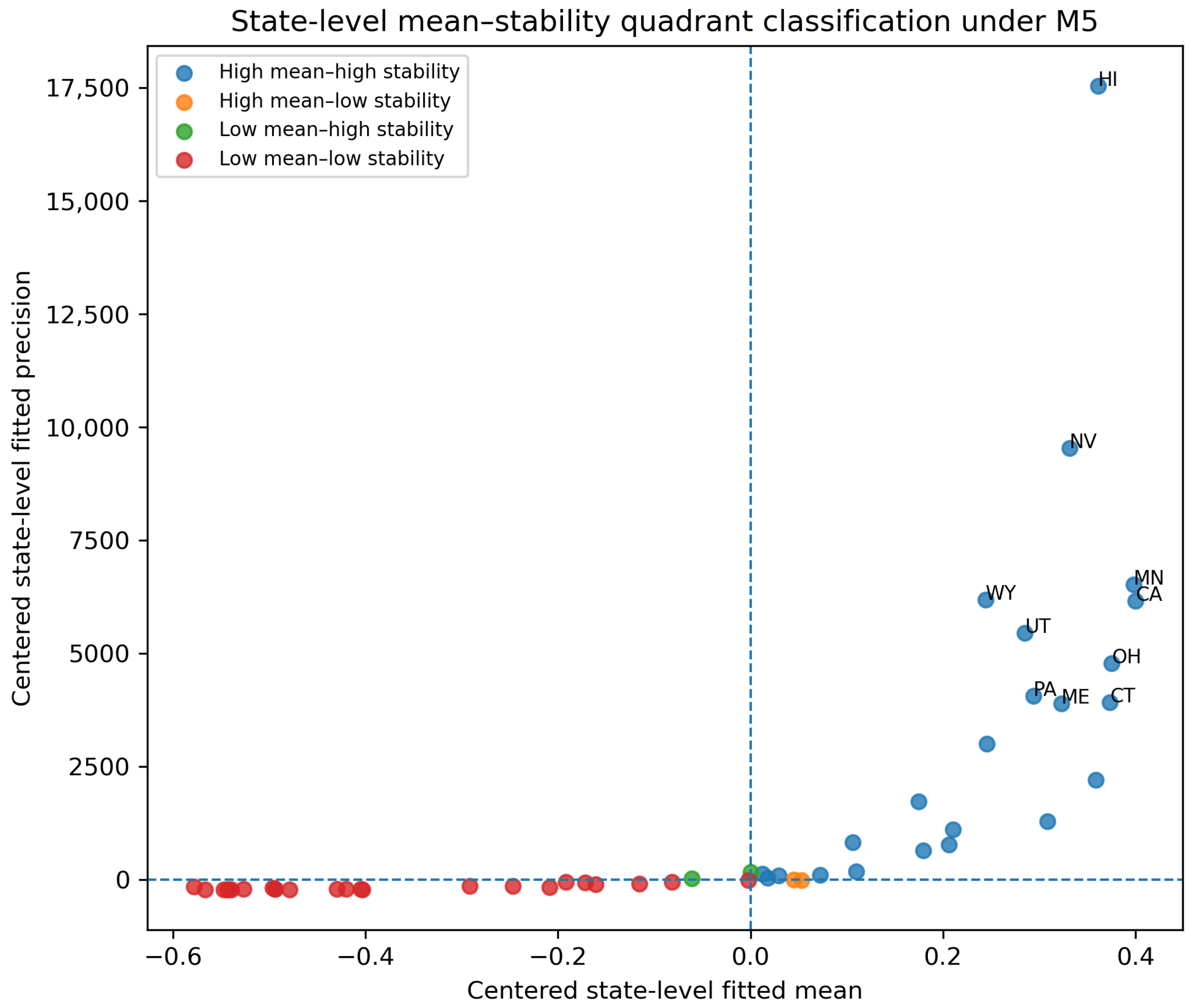
These estimates are empirical Bayes estimates. The value ${\widehat{b}}_i$ is interpreted as the adjusted latent mean-level score of cluster i, and ${\widehat{c}}_i$ is interpreted as the adjusted latent stability score of cluster i. The word adjusted means that these scores are obtained after controlling for observed covariates and nonlinear smooth effects in both submodels [11,13]. Since larger precision corresponds to smaller conditional variance, a larger value of ${\widehat{c}}_i$ indicates greater stability. When classification uncertainty is of interest, the posterior covariance matrix of $r_i$ can be approximated by $H_i{\left(\widehat{\theta }\right)}^{-1}$. This approximation allows uncertainty bands or probabilistic quadrant assignment to be constructed for the cluster-level mean–stability classification. Let ${\tau }_b$ and ${\tau }_c$ be thresholds for the latent mean-level and stability scores. They can be chosen as zero or as the empirical medians of ${\left\{{\widehat{b}}_i\right\}}_{i=1}^m$ and ${\left\{{\widehat{c}}_i\right\}}_{i=1}^m$. Cluster i is classified as high mean–high stability if

$${\widehat{b}}_i>{\tau }_b,{\widehat{c}}_i>{\tau }_c.$$

(82)

It is classified as high mean–low stability if

$${\widehat{b}}_i>{\tau }_b,{\widehat{c}}_i\le {\tau }_c.$$

(83)

It is classified as low mean–high stability if

$${\widehat{b}}_i\le {\tau }_b,{\widehat{c}}_i>{\tau }_c.$$

(84)

It is classified as low mean–low stability if

$${\widehat{b}}_i\le {\tau }_b,{\widehat{c}}_i\le {\tau }_c.$$

(85)

This classification separates clusters with high and stable proportions from those with high but unstable proportions. It also distinguishes clusters with consistently low proportions from clusters whose low average levels are accompanied by substantial instability. Therefore, the proposed model provides not only parameter estimates but also an interpretable group-level diagnostic framework. For model comparison, let ${\widehat{\mathsf{\ell }}}_L$ denote the unpenalized Laplace-approximated marginal log-likelihood evaluated at the penalized maximum likelihood estimate. Following recent model-selection studies for generalized, additive, and Beta regressions [36,37], we define the Akaike information criterion as

$$\mathrm{AIC}=-2{\widehat{\mathsf{\ell }}}_L+2d_{\mathrm{eff}}.$$

(86)

The Bayesian information criterion replaces the AIC penalty with a logarithmic dimension penalty [36,37]. Because the marginal likelihood factorizes over independent clusters, we use the cluster-level definition

$${\mathrm{BIC}}_m=-2{\widehat{\mathsf{\ell }}}_L+d_{\mathrm{eff}}\log m.$$

(87)

If observation-level comparison is desired, one may alternatively report ${\mathrm{BIC}}_N=-2{\widehat{\mathsf{\ell }}}_L+d_{\mathrm{eff}}\log N$. In the numerical studies, $d_{\mathrm{eff}}$ is taken as the number of estimated finite-dimensional parameters for comparability across Monte Carlo replications. A sensitivity analysis using spline effective degrees of freedom may be reported as a robustness check. Because penalized splines are included, this choice should be interpreted as a working information criterion rather than a full effective-degrees-of-freedom correction. The same counting rule is applied across all competing semiparametric models to maintain comparability [38]. The main competing models include the classical Beta regression with constant precision, the varying-precision Beta regression without random effects, the Beta mixed model with a random effect only in the mean submodel, the independent mean–precision random-effects Beta model with $\rho =0$, and the proposed correlated mean–precision random-effects Beta model. For an existing cluster i, conditional prediction uses the empirical Bayes estimates of the random effects. The predicted mean is

$${\widehat{\mu }}_{ij}={\displaystyle \frac{\exp \left({\widehat{\eta }}_{ij}^{\mu }\right)}{1+\exp \left({\widehat{\eta }}_{ij}^{\mu }\right)}},$$

(88)

where

$${\widehat{\eta }}_{ij}^{\mu }=x_{ij}^{\top }\widehat{\beta }+B{\left(w_{ij}\right)}^{\top }\widehat{\alpha }+{\widehat{b}}_i.$$

(89)

The predicted precision is

$${\widehat{\varphi }}_{ij}=\exp \left({\widehat{\eta }}_{ij}^{\varphi }\right),$$

(90)

where

$${\widehat{\eta }}_{ij}^{\varphi }=z_{ij}^{\top }\widehat{\gamma }+C{\left(s_{ij}\right)}^{\top }\widehat{\delta }+{\widehat{c}}_i.$$

(91)

The fitted predictive distribution is

$$Y_{ij}^{\mathrm{pred}}\sim \mathrm{Beta}\left({\widehat{\mu }}_{ij}{\widehat{\varphi }}_{ij},(1-{\widehat{\mu }}_{ij}){\widehat{\varphi }}_{ij}\right).$$

(92)

For a new cluster with no prior observations, marginal prediction can be obtained by setting $b_i=0$ and $c_i=0$ to obtain population-level predictions, or by simulating ${(b_i,c_i)}^{\top }$ from the fitted bivariate normal distribution with covariance matrix $\widehat{\mathrm{\Sigma }}$. Conditional prediction is therefore used for clusters already observed in the data, whereas marginal prediction is used for new clusters.

4. Simulation Studies

4.1. Simulation Design

Monte Carlo simulation studies were conducted to evaluate the finite-sample performance of the proposed correlated mean–precision random-effects Beta regression model. The simulation study was designed to examine five aspects of the proposed method: the recovery of the conditional mean component, the recovery of the conditional precision component, the estimation and testing of the latent mean–stability correlation $\rho$, the recovery of cluster-level random effects, and the out-of-sample predictive performance compared with nested Beta regression-type models and mainstream machine-learning predictors. For each simulated dataset, clustered proportion responses were generated from the model introduced in Section 2. Let $i=1,\dots ,m$ denote the cluster index and $j=1,\dots ,n_i$ denote the within-cluster observation index. Conditional on the cluster-level random effects $b_i$ and $c_i$, the response was generated as

$$Y_{ij}\mid b_i,c_i\sim \mathrm{Beta}\{{\mu }_{ij}{\varphi }_{ij},(1-{\mu }_{ij}){\varphi }_{ij}\}.$$

(93)

The conditional mean and precision were specified by

$$\mathrm{logit}\left({\mu }_{ij}\right)=x_{ij}^{\top }\beta +f\left(w_{ij}\right)+b_i,$$

(94)

and

$$\log \left({\varphi }_{ij}\right)=z_{ij}^{\top }\gamma +g\left(s_{ij}\right)+c_i.$$

(95)

The cluster-level random effects followed

$$\left(\begin{array}{c}{b}_i\\ c_i\end{array}\right)\sim N_2\left[\left(\begin{array}{c}0\\ 0\end{array}\right),\left(\begin{array}{cc}{\sigma }_b^2& \rho {\sigma }_b{\sigma }_c\\ \rho {\sigma }_b{\sigma }_c& {\sigma }_c^2\end{array}\right)\right].$$

(96)

The covariate vectors were $x_{ij}={(1,x_{1ij},x_{2ij})}^{\top }$ and $z_{ij}={(1,z_{1ij},z_{2ij})}^{\top }$, where

$$x_{1ij},z_{1ij}\sim N(0,1),x_{2ij},z_{2ij}\sim U(-1,1).$$

(97)

The nonlinear covariates were independently generated as

$$w_{ij},s_{ij}\sim U(0,1).$$

(98)

The true fixed-effect coefficients were

$$\beta ={(0.30,0.80,-0.60)}^{\top },\gamma ={(1.00,0.50,-0.40)}^{\top }.$$

(99)

The baseline nonlinear functions were

$$f\left(w\right)=0.50\sin \left(2\pi w\right),g\left(s\right)=0.40\cos \left(2\pi s\right).$$

(100)

The baseline random-effect standard deviations were

$${\sigma }_b=0.50,{\sigma }_c=0.40.$$

(101)

To examine different directions and strengths of the latent association between group-specific mean level and group-specific stability, the correlation parameter was set as

$$\rho \in \{-0.60,-0.30,0,0.30,0.60\}.$$

(102)

The cases $\rho =0.30$ and $\rho =0.60$ represent weak and strong positive latent associations, whereas $\rho =-0.30$ and $\rho =-0.60$ represent weak and strong negative latent associations. The case $\rho =0$ was included to examine whether the likelihood-ratio test maintains an appropriate false positive rate when the two random effects are truly independent. To evaluate the effects of the number of clusters and the number of observations within clusters, we considered

$$m\in \{50,100,200\},n_i=n\in \{5,10,20\}.$$

(103)

Thus, each simulation setting was balanced and had total sample size $N=mn$. Unless otherwise stated, the baseline sample size was $m=100$ and $n=10$. Each simulation setting was independently repeated $B_{\mathrm{mc}}=50$ times. Several supplementary settings were considered. First, to examine the impact of between-cluster heterogeneity, we used

$$({\sigma }_b,{\sigma }_c)\in \{(0.30,0.30),(0.50,0.40),(0.80,0.60)\}.$$

(104)

Second, to evaluate the semiparametric smooth components under different nonlinear structures, four function cases were considered:

$$\begin{array}{cc}\mathrm{Case}\mathrm{I}:\hfill & f\left(w\right)=0.50\sin \left(2\pi w\right),g\left(s\right)=0.40\cos \left(2\pi s\right),\hfill \\ \mathrm{Case}\mathrm{II}:\hfill & f\left(w\right)=0.60\{{(w-0.50)}^2-1/12\},g\left(s\right)=0.50\sin \left(\pi s\right)-1/\pi ,\hfill \\ \mathrm{Case}\mathrm{III}:\hfill & f\left(w\right)=0.40\{\exp (w-0.50)-(e^{0.5}-e^{-0.5})\},g\left(s\right)=0.30(s^2-1/3),\hfill \\ \mathrm{Case}\mathrm{IV}:\hfill & f\left(w\right)=0,g\left(s\right)=0.\hfill \end{array}$$

(105)

Case I is the baseline nonlinear setting. Cases II and III represent alternative nonlinear shapes, while Case IV corresponds to a purely linear data-generating mechanism. Third, two boundary settings were considered. In the mean-only boundary setting, the data were generated with ${\sigma }_c=0$, so that only the mean random effect was present. In the precision-only boundary setting, the data were generated with ${\sigma }_b=0$, so that only the precision random effect was present. In both boundary cases, the correlation parameter $\rho$ is not identifiable in the data-generating process. Five Beta regression-type models were fitted to each simulated dataset. The competing models are summarized in

Table 2. Competing Beta regression-type models fitted in the simulation study.

Model	Mean Submodel	Precision Submodel and Random-Effect Structure
M1	$\mathrm{logit}\left({\mu }_{ij}\right)=x_{ij}^{\top }\beta$	${\varphi }_{ij}=\varphi$
M2	$\mathrm{logit}\left({\mu }_{ij}\right)=x_{ij}^{\top }\beta +f\left(w_{ij}\right)$	$\log \left({\varphi }_{ij}\right)=z_{ij}^{\top }\gamma +g\left(s_{ij}\right)$
M3	$\mathrm{logit}\left({\mu }_{ij}\right)=x_{ij}^{\top }\beta +f\left(w_{ij}\right)+b_i$	$\log \left({\varphi }_{ij}\right)=z_{ij}^{\top }\gamma +g\left(s_{ij}\right)$
M4	$\mathrm{logit}\left({\mu }_{ij}\right)=x_{ij}^{\top }\beta +f\left(w_{ij}\right)+b_i$	$\log \left({\varphi }_{ij}\right)=z_{ij}^{\top }\gamma +g\left(s_{ij}\right)+c_i$, $b_i\perp c_i$
M5	$\mathrm{logit}\left({\mu }_{ij}\right)=x_{ij}^{\top }\beta +f\left(w_{ij}\right)+b_i$	$\log \left({\varphi }_{ij}\right)=z_{ij}^{\top }\gamma +g\left(s_{ij}\right)+c_i$, $\mathrm{Corr}(b_i,c_i)=\rho$

. Model M4 is the most important nested competitor because it is obtained from M5 by imposing $\rho =0$.

For all models involving smooth functions, cubic B-spline bases were used. In the implementation, $K_f=K_g=8$ basis functions were used, and second-order difference penalties were imposed on the spline coefficients. To make the model comparison stable across Monte Carlo replications, the smoothing parameters were fixed at ${\lambda }_f={\lambda }_g=1$ in the main simulation. Random effects were integrated out using the Laplace approximation described in Section 3, and the finite-dimensional parameters were estimated using the quasi-Newton optimization procedure. In addition to the five Beta regression-type models, four mainstream machine-learning regressors were included for train/test point-prediction comparison: decision tree, random forest, gradient boosting, and K-nearest neighbors. These benchmark methods were fitted using the covariates $(x_{1ij},x_{2ij},z_{1ij},z_{2ij},w_{ij},$ and $s_{ij})$ as predictors and $Y_{ij}$ as the response. The random forest and gradient boosting regressors used 100 trees or boosting iterations, the minimum leaf size was set to 5, and the K-nearest-neighbor model used $K=10$. These machine-learning methods were used only as point-prediction benchmarks; they do not provide estimates of ${\varphi }_{ij}$, $\rho$, cluster-level random effects, or Beta likelihood-based criteria [11,13].

4.2. Evaluation Criteria

The evaluation criteria were divided into five groups. RMSE and MAE follow their recent SCI model-evaluation definitions [39], while NLPD is the negative logarithmic score, a strictly proper density score [40]. Because a continuous density may exceed one, its logarithm may be positive and an average NLPD may be negative; smaller values remain better. First, we evaluated the estimation accuracy of finite-dimensional parameters. For a generic parameter vector ${\theta }_0$ and its estimator ${\widehat{\theta }}^{\left(r\right)}$ in the r-th Monte Carlo replication, the empirical bias and root mean squared error are defined as

$$\mathrm{Bias}\left(\widehat{\theta }\right)={\displaystyle \frac{1}{B_{\mathrm{mc}}}}{\displaystyle \sum _{r=1}^{B_{\mathrm{mc}}}}\left({\widehat{\theta }}^{\left(r\right)}-{\theta }_0\right),$$

(106)

and

$$\mathrm{RMSE}\left(\widehat{\theta }\right)={\left[{\displaystyle \frac{1}{B_{\mathrm{mc}}}}{\displaystyle \sum _{r=1}^{B_{\mathrm{mc}}}}{∥{\widehat{\theta }}^{\left(r\right)}-{\theta }_0∥}_2^2\right]}^{1/2}.$$

(107)

These quantities were reported for $\beta$, $\gamma$, and $\rho$ whenever the corresponding parameters were included and identifiable. Second, we evaluated the recovery of the latent conditional mean and precision. Let ${\widehat{\mu }}_{ij}^{\left(r\right)}$ and ${\widehat{\varphi }}_{ij}^{\left(r\right)}$ denote the fitted conditional mean and precision in the r-th replication. The in-sample recovery errors were defined as

$${\mathrm{RMSE}}_{\mu }={\left[{\displaystyle \frac{1}{B_{\mathrm{mc}}}}{\displaystyle \sum _{r=1}^{B_{\mathrm{mc}}}}{\displaystyle \frac{1}{N}}{\displaystyle \sum _{i=1}^m}{\displaystyle \sum _{j=1}^{n_i}}{\left({\widehat{\mu }}_{ij}^{\left(r\right)}-{\mu }_{ij}^{\left(r\right)}\right)}^2\right]}^{1/2},$$

(108)

and

$${\mathrm{RMSE}}_{\varphi }={\left[{\displaystyle \frac{1}{B_{\mathrm{mc}}}}{\displaystyle \sum _{r=1}^{B_{\mathrm{mc}}}}{\displaystyle \frac{1}{N}}{\displaystyle \sum _{i=1}^m}{\displaystyle \sum _{j=1}^{n_i}}{\left({\widehat{\varphi }}_{ij}^{\left(r\right)}-{\varphi }_{ij}^{\left(r\right)}\right)}^2\right]}^{1/2}.$$

(109)

Third, inference on the mean–stability association was assessed through the likelihood-ratio test comparing M5 with M4. Since M4 is obtained from M5 by setting $\rho =0$, the likelihood-ratio statistic was

$$T_{\mathrm{LR}}=2\{{\mathsf{\ell }}_L\left({\widehat{\theta }}_{\mathrm{M}5}\right)-{\mathsf{\ell }}_L\left({\widehat{\theta }}_{\mathrm{M}4}\right)\},$$

(110)

where ${\mathsf{\ell }}_L(·)$ denotes the unpenalized Laplace-approximated marginal log-likelihood. Under the null hypothesis $H_0:\rho =0$, the test statistic was compared with a ${\chi }_1^2$ reference distribution. The empirical rejection rate at the $5\%$ level was recorded. Fourth, likelihood-based fit and distributional prediction were evaluated using AIC, cluster-level BIC, and the negative log predictive density. The cluster-level BIC was computed as

$${\mathrm{BIC}}_m=-2{\mathsf{\ell }}_L\left(\widehat{\theta }\right)+d\log m,$$

(111)

where d is the number of estimated finite-dimensional parameters. The full-data negative log predictive density was

$${\mathrm{NLPD}}_{\mathrm{full}}=-{\displaystyle \frac{1}{N}}{\displaystyle \sum _{i=1}^m}{\displaystyle \sum _{j=1}^{n_i}}\log p_{\mathrm{B}}\left(Y_{ij}\mid {\widehat{\mu }}_{ij},{\widehat{\varphi }}_{ij}\right),$$

(112)

where $p_{\mathrm{B}}(·\mid \mu ,\varphi )$ denotes the Beta density under the mean–precision parameterization. Fifth, train/test prediction was evaluated by holding out $30\%$ of the clusters as test clusters. Because the test clusters were not observed during training, the prediction for M1–M5 used population-level random effects for the held-out clusters. The test-set mean squared prediction error and root mean squared prediction error were defined as

$${\mathrm{MSPE}}_{\mathrm{test}}={\displaystyle \frac{1}{N_{\mathrm{test}}}}\sum _{(i,j)\in \mathcal{T}}{\left(Y_{ij}-{\widehat{\mu }}_{ij}\right)}^2,$$

(113)

and

$${\mathrm{RMSE}}_{Y,\mathrm{test}}={\left[{\displaystyle \frac{1}{N_{\mathrm{test}}}}\sum _{(i,j)\in \mathcal{T}}{\left(Y_{ij}-{\widehat{\mu }}_{ij}\right)}^2\right]}^{1/2},$$

(114)

where $\mathcal{T}$ denotes the test set. For the Beta regression-type models, test-set NLPD was also computed using the fitted Beta density.

4.3. Simulation Results

A fit was regarded as numerically successful if the optimizer returned a finite objective value, the fitted variance components were positive, the fitted correlation satisfied $|\widehat{\rho }|<1$, the Laplace Hessian matrices were positive definite after the prescribed ridge stabilization, and the fitted ${\widehat{\mu }}_{ij}$ and ${\widehat{\varphi }}_{ij}$ were finite for all observations. Under this criterion, all reported simulation runs were numerically successful. The raw simulation output contained $23\times 50\times 9=$ 10,350 fitted model records, corresponding to 23 simulation settings, 50 Monte Carlo replications, five Beta regression-type models, and four machine-learning benchmark models.

4.3.1. Overall Performance of the Beta Regression-Type Models

Table 3. Average performance of M1–M5 across the 23 simulation settings, with 50 Monte Carlo replications per setting. Metrics are first computed within each fitted dataset and then averaged across settings and replications. Bold marks the best values for the five recovery and full-data model-selection criteria. Test-set MSPE and NLPD evaluate new-cluster transportability; success equals 1.00 for every model.

Model	${\mathrm{RMSE}}_{\mathit{\mu }}$	${\mathrm{RMSE}}_{\mathit{\varphi }}$	NLPDfull	MSPEtest	NLPDtest	AIC	BICm	Success
M1	0.1219	3.5407	−0.4722	0.0741	−0.4606	−1066.48	−1056.06	1.00
M2	0.1006	2.3332	−0.6230	0.0699	−0.5904	−1372.59	−1315.28	1.00
M3	0.0588	1.9136	−0.7598	0.0698	−0.5609	−1483.99	−1424.07	1.00
M4	0.0574	1.4647	−0.8257	0.0698	−0.5574	−1515.50	−1452.97	1.00
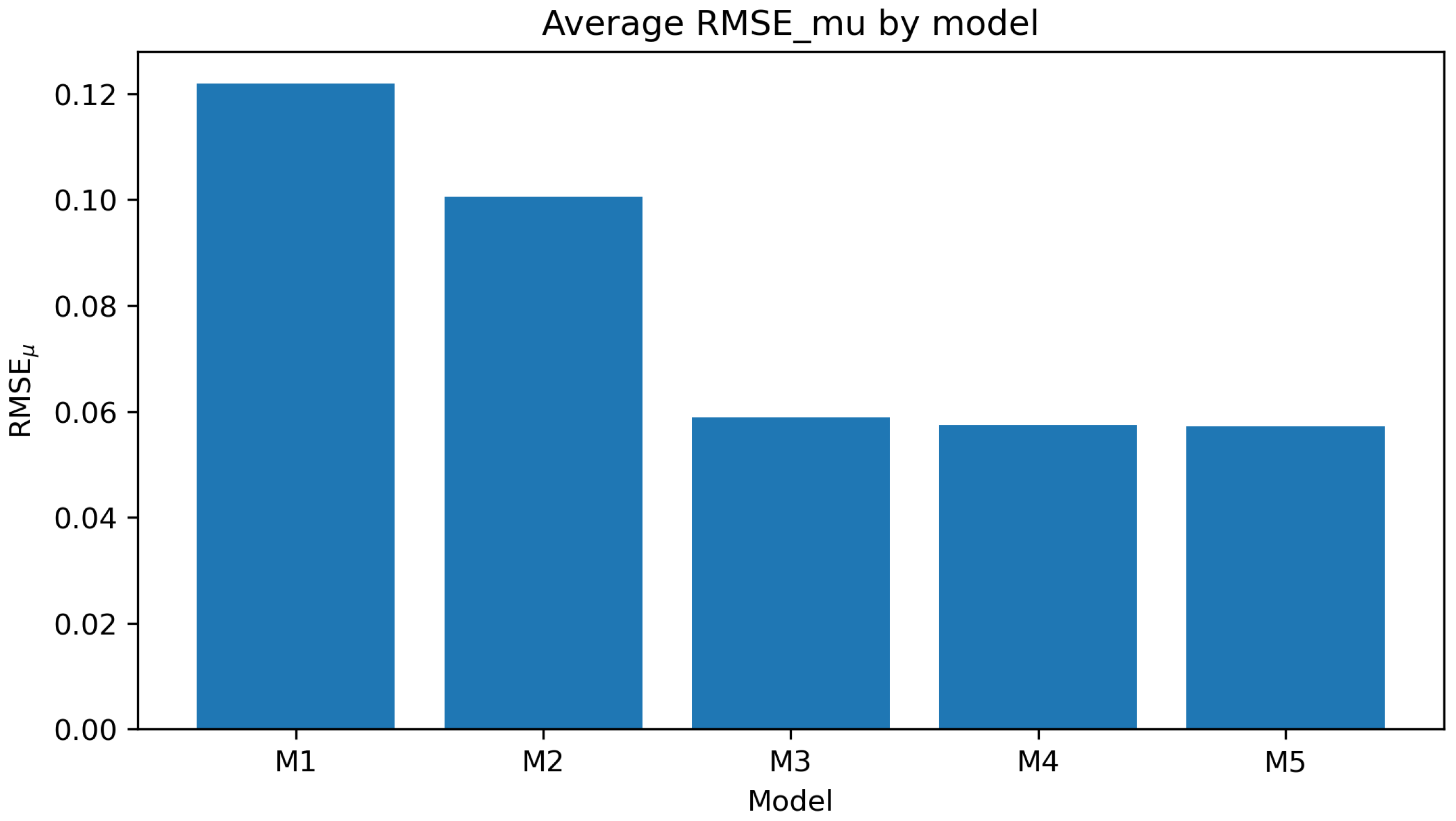
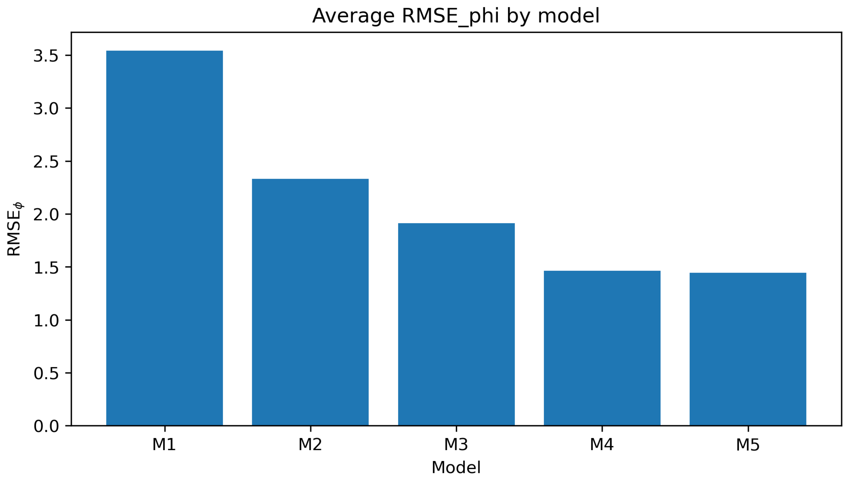
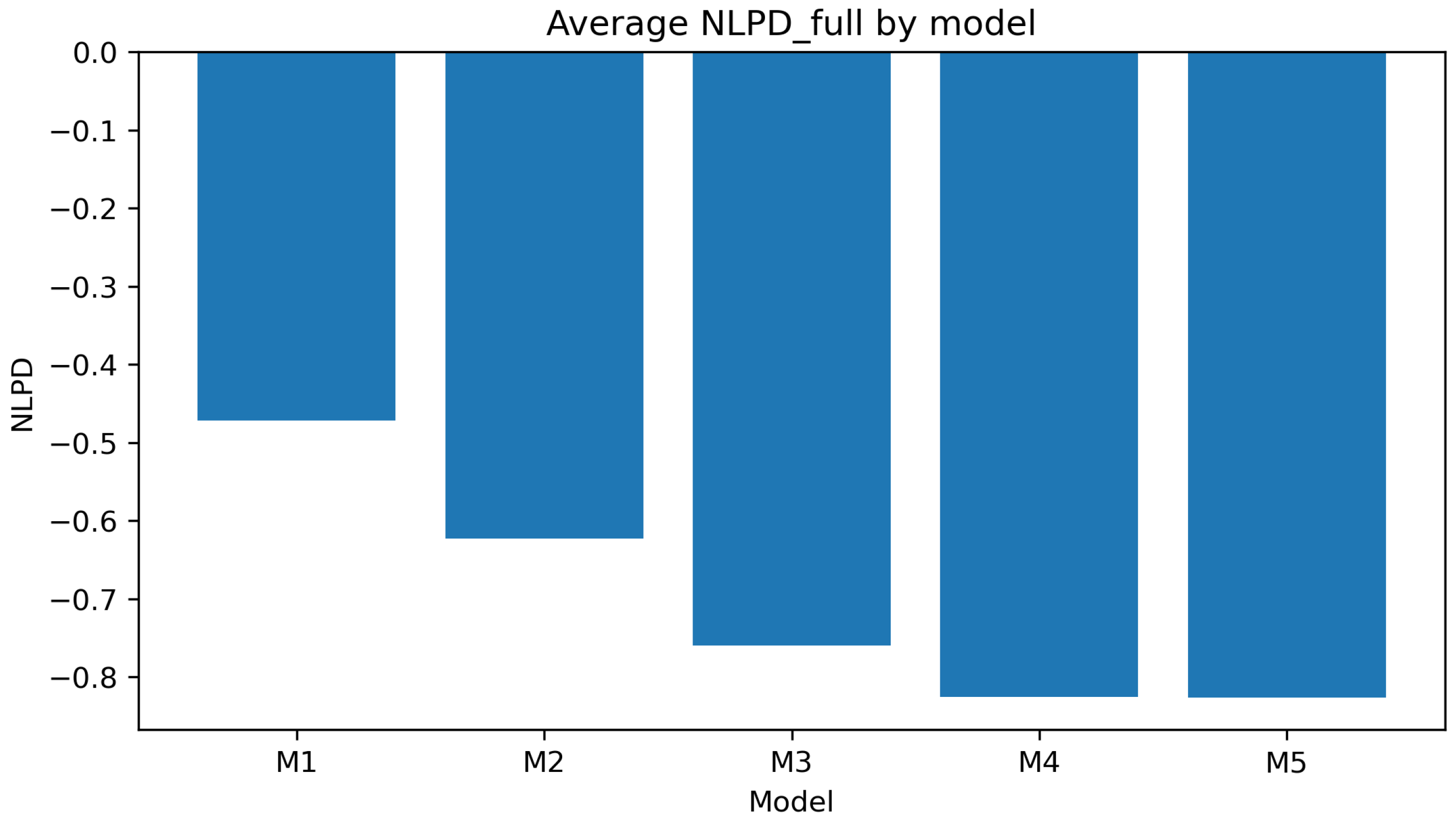
M5	0.0571	1.4455	−0.8260	0.0699	−0.5575	−1518.11	−1452.99	1.00

reports the average performance of M1–M5 across all simulation settings. M1, which assumes constant precision and ignores cluster heterogeneity, has the largest errors in both $\mu$ and $\varphi$. Modeling precision in M2 and adding random effects in M3 and M4 improve recovery and fit. M5, which also models dependence between the two random effects, has the smallest average ${\mathrm{RMSE}}_{\mu }$, ${\mathrm{RMSE}}_{\varphi }$, AIC, BIC_m, and ${\mathrm{NLPD}}_{\mathrm{full}}$. On the combined recovery, fit, and inferential criteria used here, M5 is the best overall Beta regression-type model. The held-out scores evaluate prediction for new clusters. M5 is comparable to the leading models on that target and also provides a formal test of dependence and a cluster-level interpretation of $\rho$.

Figure 2, Figure 3 and Figure 4 summarize the average recovery of $\mu$ and $\varphi$ and the full-data density score. M5 has the lowest average value in all three displays. Its advantage in ${\mathrm{RMSE}}_{\varphi }$ is consistent with modeling cluster-specific stability heterogeneity together with its dependence on mean heterogeneity.

4.3.2. Recovery and Testing of the Mean–Stability Correlation

Table 4. Recovery of $\rho$ and empirical rejection of the M5-versus-M4 LRT in the five baseline settings ($m=100$, $n_i=10$, 50 replications). Parentheses give 95% Wilson intervals for the rejection proportion, quantifying Monte Carlo uncertainty.

True $\mathit{\rho }$	Bias $\left(\widehat{\mathit{\rho }}\right)$	RMSE $\left(\widehat{\mathit{\rho }}\right)$	LRT Rejection Rate	95% Wilson Interval
−0.60	−0.0031	0.1074	0.94	(0.838, 0.979)
−0.30	−0.0029	0.1575	0.26	(0.159, 0.396)
0.00	−0.0087	0.2016	0.04	(0.011, 0.135)
0.30	−0.0244	0.1929	0.38	(0.259, 0.518)
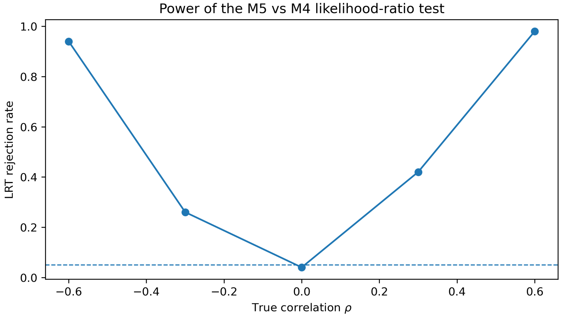
0.60	0.0073	0.1201	0.98	(0.895, 0.996)

reports the recovery of $\rho$ under the baseline sample size $m=100$ and $n=10$. The proposed M5 estimates $\rho$ with small empirical bias across all five baseline correlation settings. When $\rho =-0.60$ and $\rho =0.60$, the likelihood-ratio test has high empirical rejection rates, 0.94 and 0.98, respectively. Because each setting was repeated $B_{\mathrm{mc}}=50$ times, the Monte Carlo standard error of an empirical rejection rate $\widehat{p}$ is approximately ${\{\widehat{p}(1-\widehat{p})/50\}}^{1/2}$. For example, when $\rho =0$, the empirical rejection rate is 0.04 and the corresponding Monte Carlo standard error is approximately 0.0277. Therefore, the rejection rate should be interpreted as being close to the nominal level rather than as an exact estimate of the type I error probability. When $\rho =0$, the rejection rate is 0.04, close to the nominal $5\%$ level. For the weak association settings $\rho =-0.30$ and $\rho =0.30$, the rejection rates are lower, which is consistent with the difficulty of detecting weak latent correlations in finite samples.

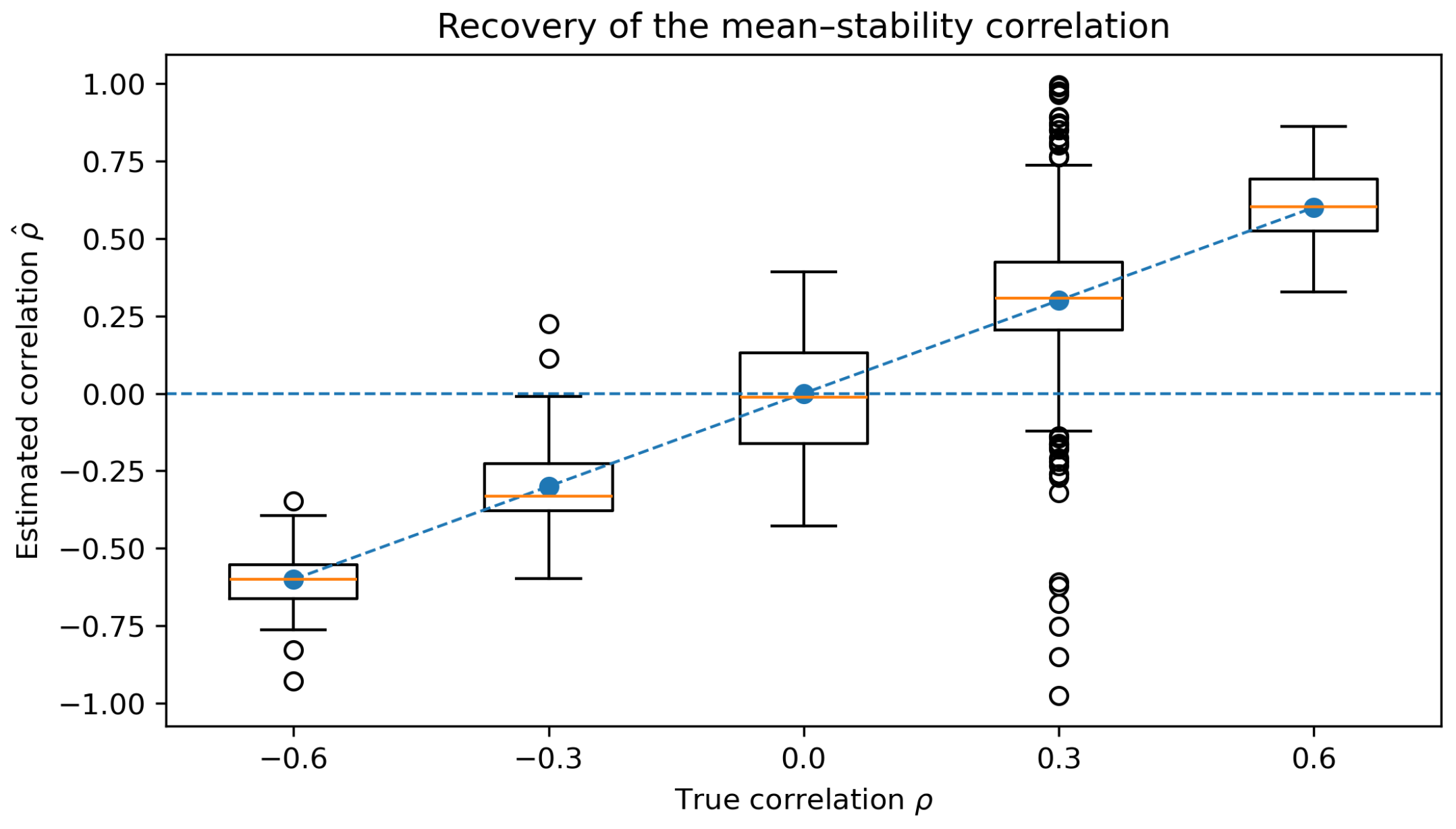
Figure 5 and Figure 6 provide graphical summaries. The boxplot shows that $\widehat{\rho }$ tracks the true value of $\rho$ reasonably well. The empirical power curve confirms that strong positive and negative latent associations are detected with high probability, while the type I error under $\rho =0$ remains close to the nominal level.

4.3.3. Direct Comparison Between M5 and M4

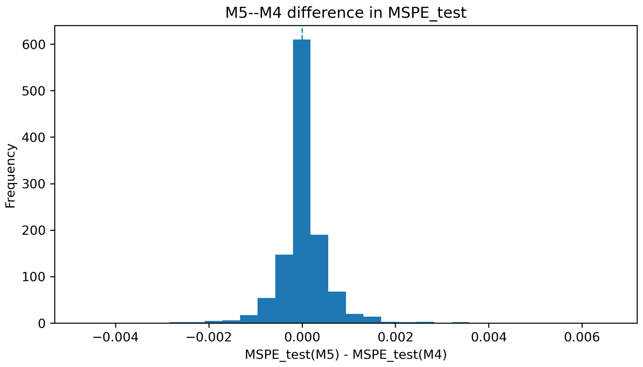
Because M4 is the independent mean–precision random-effects model and is nested within M5, the comparison between M5 and M4 directly evaluates the value of modeling $\rho$.

Table 5. Direct comparison between M5 and M4. The reported difference is $\mathrm{\Delta }=\mathrm{criterion}\left(\mathrm{M}5\right)-\mathrm{criterion}\left(\mathrm{M}4\right)$. Negative values favor M5.

Criterion	Mean $\mathbf{\Delta }$	Median $\mathbf{\Delta }$	$Pr(\mathbf{\Delta }<0)$
${\mathrm{RMSE}}_{\mu }$	−0.0003	−0.0002	0.6235
${\mathrm{RMSE}}_{\varphi }$	−0.0191	−0.0159	0.6548
AIC	−2.6178	−0.8290	0.5913
BICm	−0.0126	1.7233	0.3583
NLPDfull	−0.0003	−0.0003	0.5600
MSPEtest	0.0000	0.0000	0.4826
NLPDtest	−0.0001	0.0001	0.4904

reports the average difference $\mathrm{\Delta }=\mathrm{criterion}\left(\mathrm{M}5\right)-\mathrm{criterion}\left(\mathrm{M}4\right)$ across all simulation settings and replications. Negative values favor M5. M5 improves over M4 on average in ${\mathrm{RMSE}}_{\mu }$, ${\mathrm{RMSE}}_{\varphi }$, AIC, BIC_m, NLPD_full, and NLPD_test. The largest relative improvement is observed in AIC and ${\mathrm{RMSE}}_{\varphi }$, showing that the correlated random-effects structure mainly improves likelihood-based fit and precision recovery. The MSPE difference is close to zero, indicating that M4 and M5 have nearly identical point-prediction performance for new clusters.

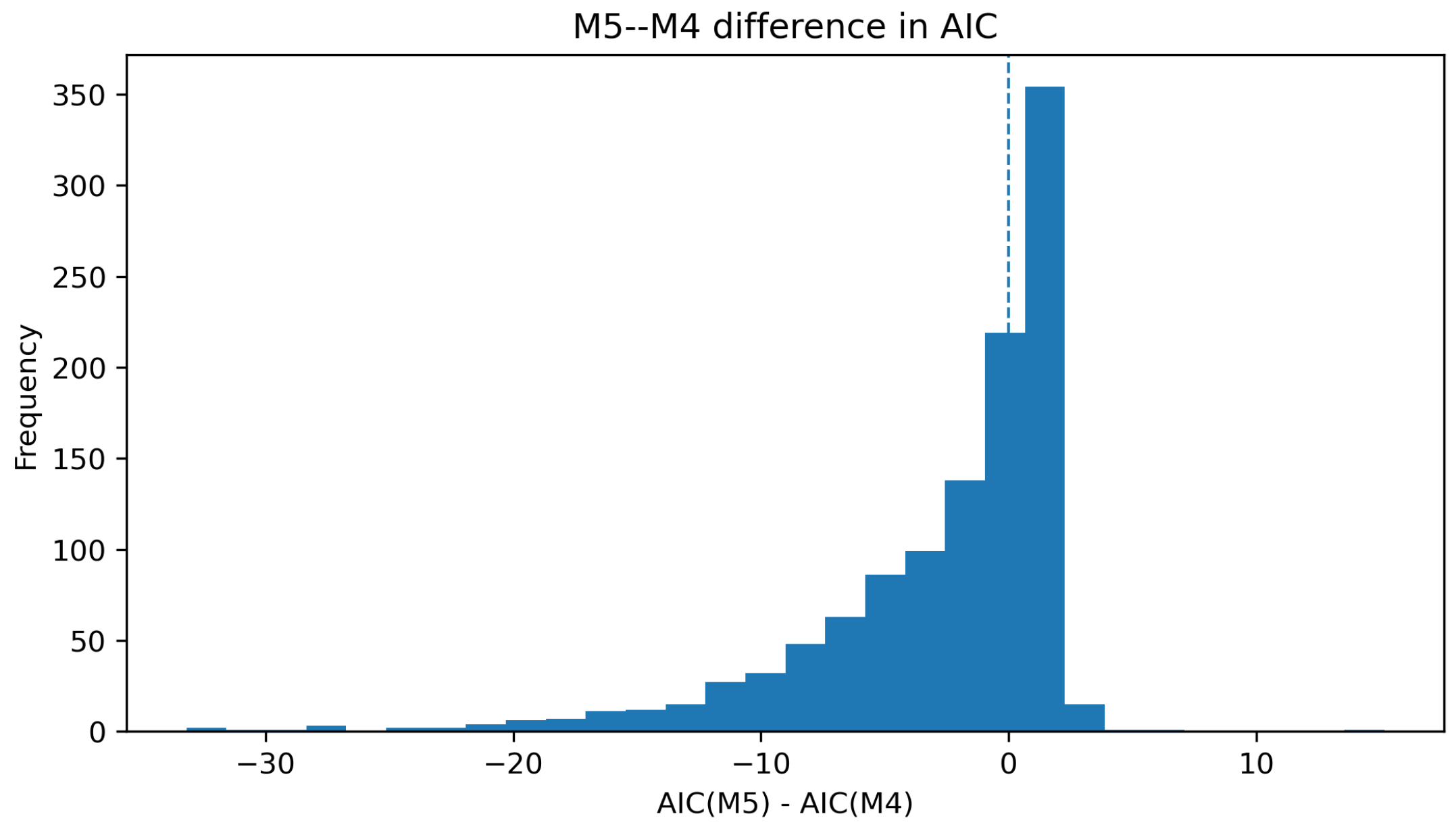
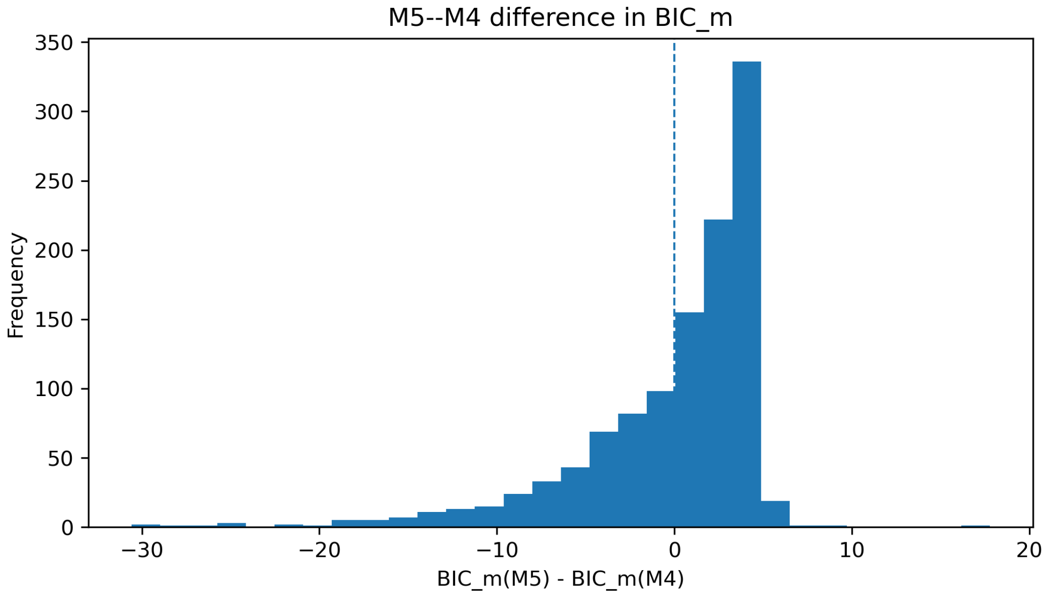
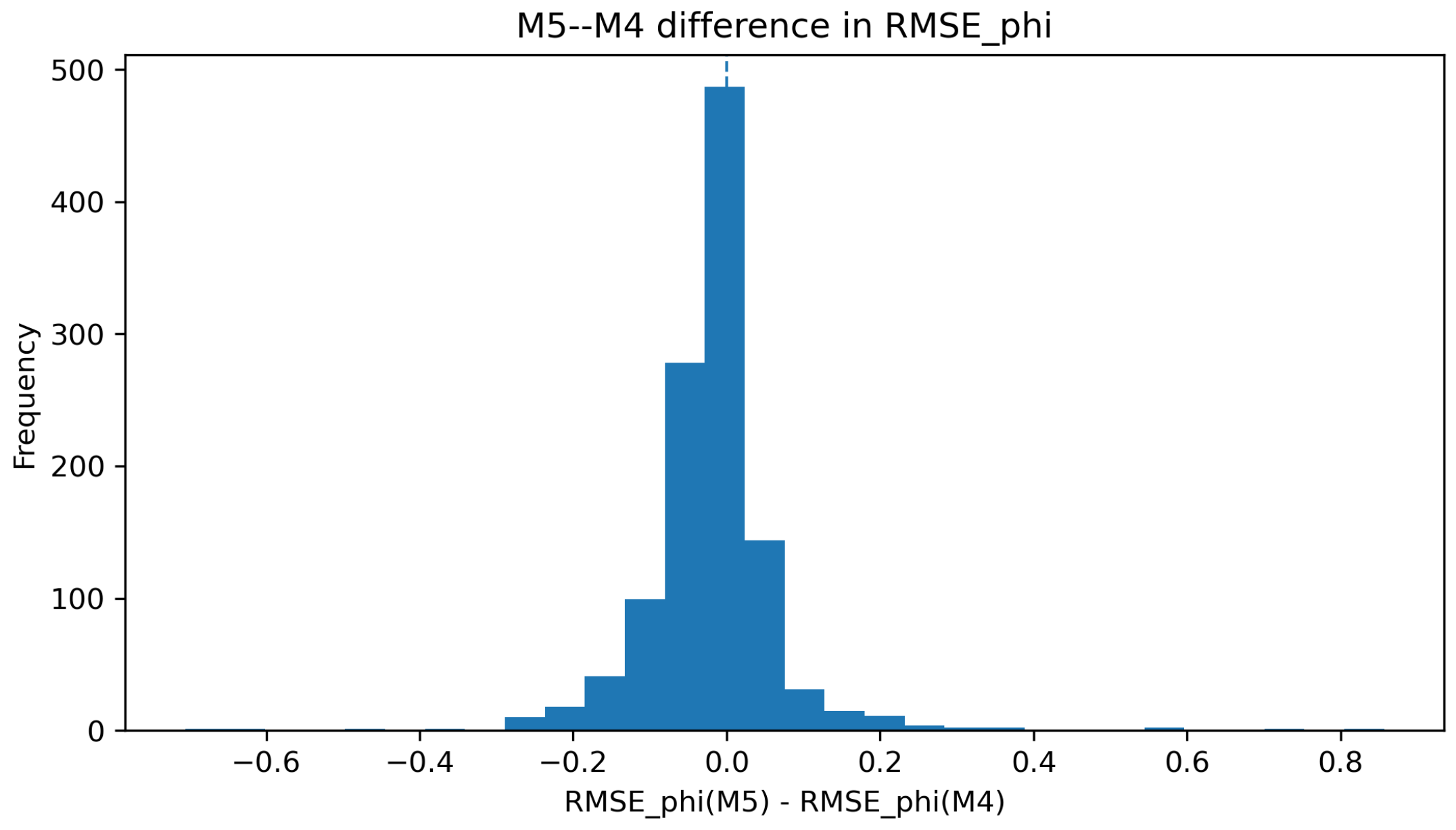
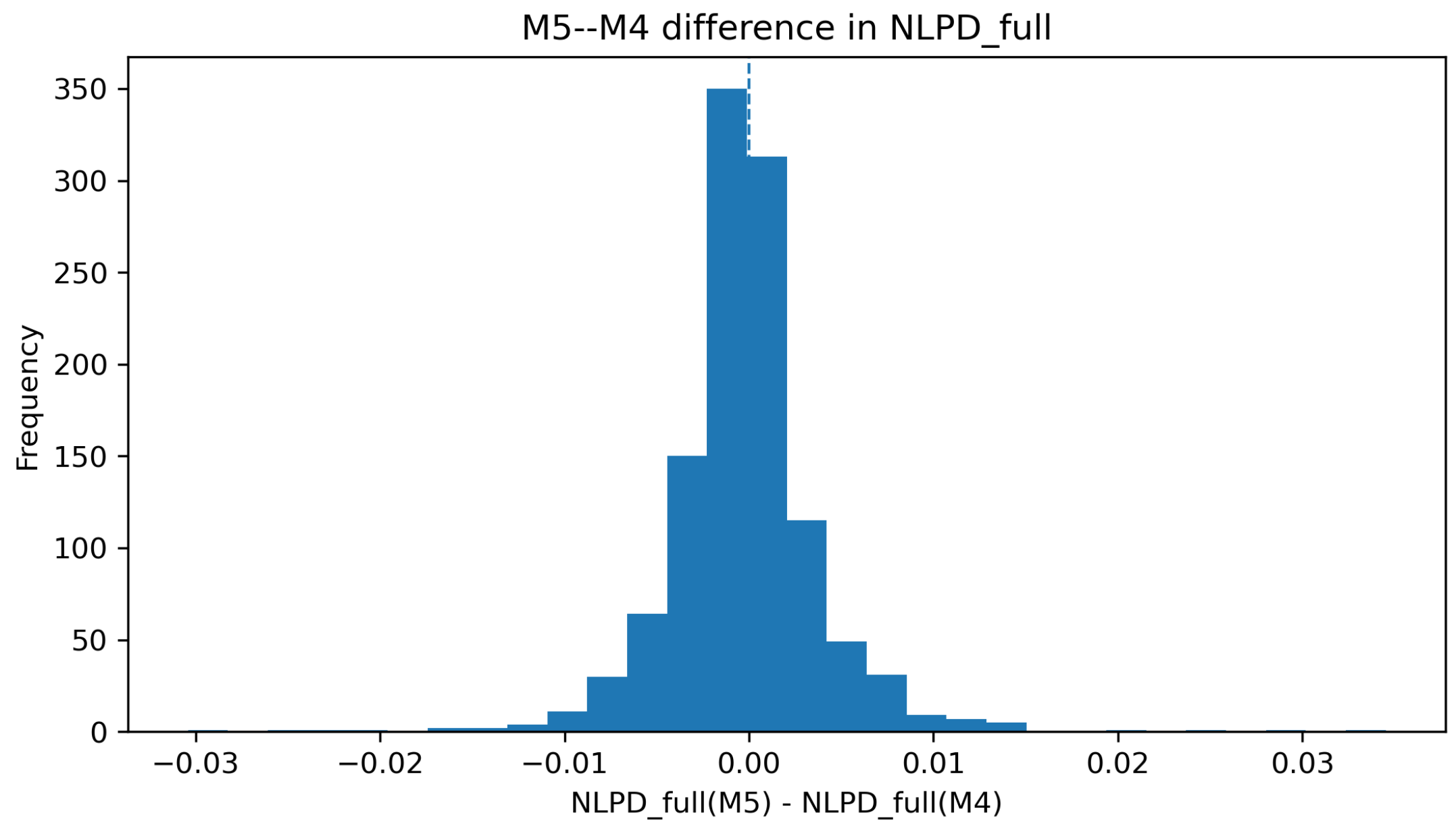
Figure 7, Figure 8, Figure 9, Figure 10 and Figure 11 show the distributions of the M5–M4 differences. The average AIC, ${\mathrm{RMSE}}_{\varphi }$, and NLPD_full differences favor M5. BIC_m imposes a stronger cluster-level penalty for the additional correlation parameter. The MSPE_test differences are concentrated near zero, so M5 retains M4’s new-cluster point-prediction accuracy while adding correlation recovery, formal inference, and paired cluster interpretation.

4.3.4. Random-Effect Recovery and Mean–Stability Classification

Table 6. Recovery of cluster-level random effects across all non-boundary simulation settings. Larger correlations, quadrant accuracy, and success rates are better; bold entries mark the best displayed value.

Model	Corr$({\mathit{b}}_{\mathit{i}},{\widehat{\mathit{b}}}_{\mathit{i}})$	Corr$({\mathit{c}}_{\mathit{i}},{\widehat{\mathit{c}}}_{\mathit{i}})$	Quadrant Accuracy	Success
M3	0.8183	–	–	1.00
M4	0.8262	0.6799	0.6060	1.00
M5	0.8266	0.6862	0.6095	1.00

summarizes the recovery of the latent random effects in non-boundary settings. M5 has the highest displayed recovery correlations for both $b_i$ and $c_i$ and the highest four-quadrant mean–stability classification accuracy. Its overall advantage thus extends to recovery and interpretation at the cluster level.

4.3.5. Boundary Settings

The boundary settings examine whether the fitted models can distinguish different sources of cluster-level heterogeneity.

Table 7. Model performance in the variance-component boundary settings, with 50 replications per setting. All displayed criteria are smaller-is-better. Bold entries identify the best value within each boundary block; comparisons are not made across the two generating mechanisms.

Boundary Setting	Model	${\mathrm{RMSE}}_{\mathit{\mu }}$	${\mathrm{RMSE}}_{\mathit{\varphi }}$	AIC	BICm	NLPDfull
Mean only	M1	0.1259	2.7962	−876.38	−865.96	−0.4422
Mean only	M2	0.1032	1.0963	−1164.78	−1107.47	−0.6044
Mean only	M3	0.0581	0.5256	−1259.70	−1199.78	−0.7506
Mean only	M4	0.0582	0.5511	−1257.96	−1195.43	−0.7551
Mean only	M5	0.0583	0.5747	−1256.75	−1191.62	−0.7555
Precision only	M1	0.0768	3.4540	−844.24	−833.81	−0.4261
Precision only	M2	0.0190	1.9016	−1179.30	−1121.99	−0.6116
Precision only	M3	0.0210	1.8901	−1178.24	−1118.32	−0.6201
Precision only	M4	0.0196	1.4123	−1208.26	−1145.73	−0.6906
Precision only	M5	0.0204	1.4263	−1207.35	−1142.22	−0.6912

reports the results for the mean-only and precision-only random-effect settings. When the data contain only a mean random effect, M3 has the smallest BIC_m, whereas M4 and M5 produce similar but slightly more complex fits. When the data contain only a precision random effect, M4 and M5 substantially reduce ${\mathrm{RMSE}}_{\varphi }$ compared with M1–M3. This confirms that the precision random effect is useful when stability heterogeneity is present, while the information criterion can still favor a simpler model when the additional random-effect structure is unnecessary.

4.3.6. Prediction Comparison with Machine-Learning Benchmarks

Table 8. Cluster-disjoint train/test prediction comparison aggregated across the simulation settings. The machine-learning models are auxiliary point-prediction benchmarks. All displayed criteria are smaller-is-better; bold entries mark the best displayed value. No $R^2$ column is shown.

Model	MSPEtest	RMSEY,test	MAEtest	RMSEμ,test	NLPDtest
M4	0.0698	0.2638	0.2158	0.1035	−0.5574
M3	0.0698	0.2639	0.2160	0.1036	−0.5609
M2	0.0699	0.2639	0.2172	0.1037	−0.5904
M5	0.0699	0.2639	0.2161	0.1037	−0.5575
M1	0.0741	0.2718	0.2259	0.1238	−0.4606
Random forest	0.0754	0.2743	0.2250	0.1287	–
Gradient boosting	0.0773	0.2776	0.2268	0.1352	–
K-nearest neighbors	0.0804	0.2832	0.2362	0.1470	–
Decision tree	0.1103	0.3316	0.2607	0.2272	–

compares test-set point prediction from M1–M5 with four standard machine-learning regressors [41,42]. M5 is in the leading group of Beta regressions, and M2–M5 outperform the four machine-learning benchmarks in this simulation design. Among the leading predictors, only M5 estimates ${\mu }_{ij}$, ${\varphi }_{ij}$, the paired random effects, and the mean–stability correlation $\rho$ together. It therefore retains strong point prediction while providing the full distributional and inferential output considered in this study.

4.3.7. Targeted Robustness, Computation, and Integration Checks

The 23-setting experiment above is the primary Monte Carlo study. A focused one-factor-at-a-time stress suite compares M4 and M5 using 30 independent replications per nonnull setting. The seed family (20260711), data-generating mechanisms, cubic B-splines with six basis functions, fixed ${\lambda }_f={\lambda }_g=1$, and optimizer settings were fixed before fitting. The fitted nested M4 point with $\xi =0$ was included among the M5 starts. The stress suite uses six basis functions for computational tractability, whereas the primary study uses eight. Except for the few-cluster and unbalanced settings, each dataset has $m=40$, $n_i=8$, and $N=320$. In the response-boundary settings, the mean linear predictor is shifted so that many continuous observations fall below 0.05 or above 0.95; no exact zeros or ones are introduced. Student-$t_5$ and 10% contaminated-mixture random effects are standardized to the target covariance before data generation, while the fitted model retains the bivariate-normal working distribution.

Table 9. Targeted M5 stress results. Every row uses $B=30$; the generating correlation is $\rho =0.6$ except in the final null row. Tail % is the observed fraction below 0.05 or above 0.95. Recovery summaries use successful M5 fits, and LRT summaries use replications in which both M4 and M5 succeeded. Coverage is for the transformed-scale 95% Wald interval. Parentheses after RMSE values are Monte Carlo standard errors; brackets after LRT rejection are 95% Wilson intervals.

Setting	m	${\mathit{n}}_{\mathit{i}}$	Tail %	Success	Bias $\left(\widehat{\mathit{\rho }}\right)$	RMSE $\left(\widehat{\mathit{\rho }}\right)$	Coverage	RMSEμ	RMSEϕ	LRT Rejection
Reference	40	8	11.9	1.000	0.018	0.198	1.000	0.0548 (0.0010)	4.205 (0.196)	0.567 [0.392, 0.726]
Few clusters	20	8	12.2	1.000	0.001	0.300	1.000	0.0639 (0.0021)	5.539 (0.705)	0.167 [0.073, 0.336]
Unbalanced clusters	40	3–20	11.9	1.000	0.003	0.248	1.000	0.0557 (0.0008)	4.201 (0.251)	0.500 [0.332, 0.668]
Responses near zero	40	8	74.8	1.000	−0.551	0.715	1.000	0.0239 (0.0005)	4.053 (0.158)	0.033 [0.006, 0.167]
Responses near one	40	8	76.4	1.000	0.313	0.420	0.967	0.0268 (0.0009)	4.715 (0.282)	0.367 [0.219, 0.545]
Low precision	40	8	38.1	1.000	0.133	0.243	1.000	0.0780 (0.0015)	0.784 (0.021)	0.633 [0.455, 0.781]
High precision	40	8	1.6	1.000	−0.224	0.353	1.000	0.0164 (0.0005)	101.389 (11.711)	0.586 [0.407, 0.745]
Student-$t_5$ random effects	40	8	12.3	1.000	−0.047	0.309	1.000	0.0550 (0.0011)	4.326 (0.235)	0.567 [0.392, 0.726]
Contaminated mixture	40	8	12.3	1.000	−0.047	0.377	1.000	0.0573 (0.0016)	4.797 (0.318)	0.533 [0.361, 0.698]
Near-zero ${\sigma }_c=0.05$	40	8	11.4	1.000	−0.495	0.815	1.000	0.0540 (0.0010)	2.147 (0.174)	0.033 [0.006, 0.167]
Near-zero ${\sigma }_c=0.05$, null †	40	8	11.3	1.000	0.117	0.664	1.000	0.0547 (0.0011)	2.777 (0.256)	0.033 [0.006, 0.167]

^† Separate $B=30$ run with generating $\rho =0$; all other rows use $B=30$ and $\rho =0.6$.

reports M5’s numerical behavior in the targeted settings. All 300 nonnull fits and all 30 fits in the separate near-zero-variance null experiment succeeded; none of the fitted covariance transforms reached its prespecified bound. As expected from Remark 1, recovery of $\rho$ was most difficult when responses were concentrated near zero and when ${\sigma }_c=0.05$. In the latter nonnull setting, $\rho$-RMSE was 0.815 and the LRT rejected once in 30 replications even though $\rho =0.6$ generated the data. In the separate null run, the ordinary ${\chi }_1^2$ LRT also rejected once (3.3%; 95% Wilson interval 0.6–16.7%). This result motivates the boundary-aware bootstrap calibration in Equation (80). All M5 fits also succeeded under the standardized $t_5$ and contaminated-mixture random-effect distributions. Monte Carlo standard errors and Wilson intervals accompany these estimates.

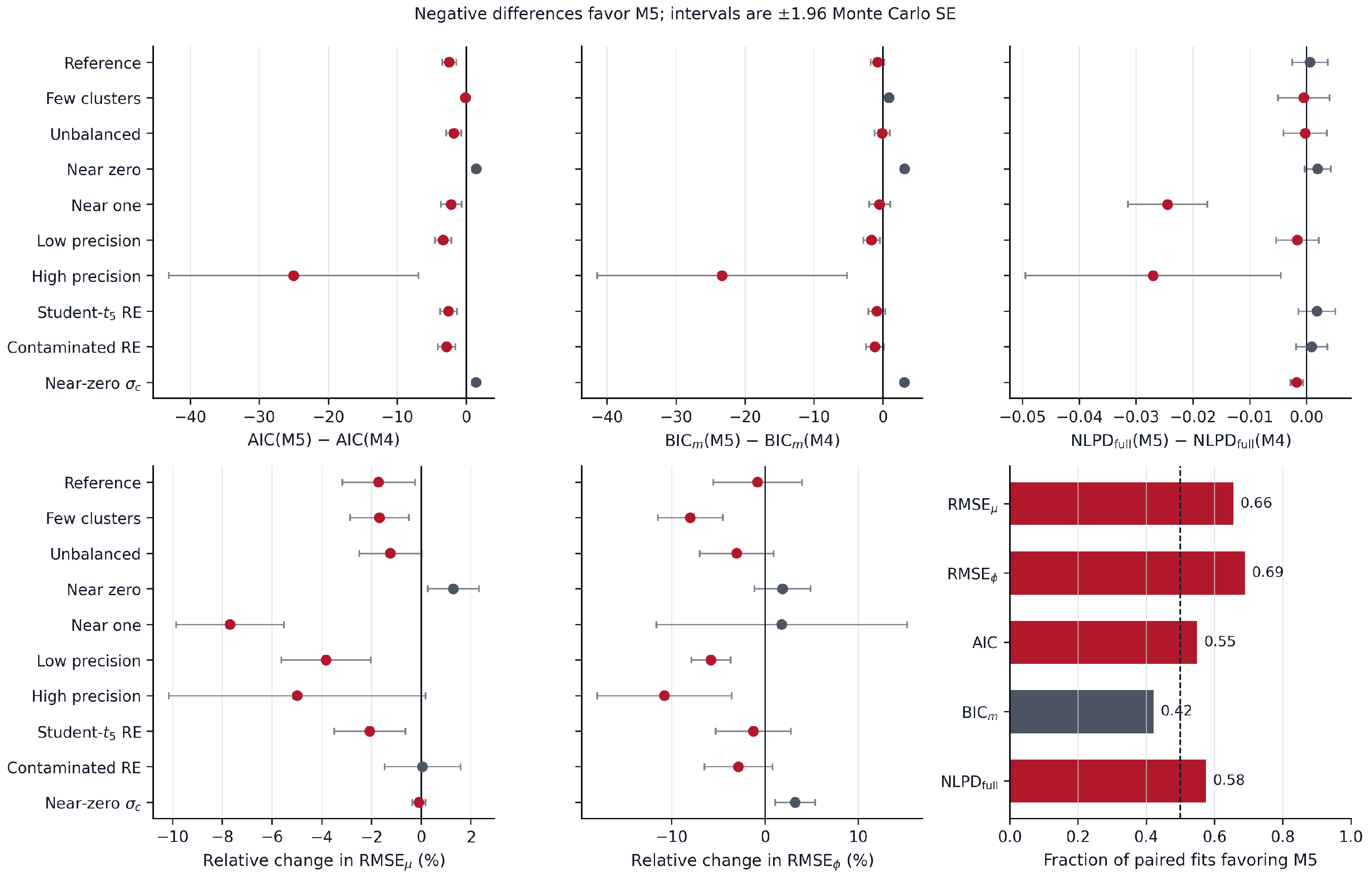
Across the 299 replications in which both models succeeded,

Table 10. Successful-pair comparison of M5 with nested M4 across the ten nonnull stress settings ($B=30$ per setting; 299 successful pairs). Recovery rows are paired relative percentage changes, while AIC, BIC_m, and NLPD rows are absolute M5-minus-M4 differences. Negative differences favor M5. Parentheses give Monte Carlo standard errors; bold marks an M5-favoring mean, median, or win fraction above 0.5.

Criterion	Mean Difference (MCSE)	Median Difference	M5 Win Fraction
Relative ${\mathrm{RMSE}}_{\mu }$ change (%)	−2.188 (0.363)	−1.001	0.656
Relative ${\mathrm{RMSE}}_{\varphi }$ change (%)	−2.550 (0.946)	−2.628	0.689
AIC	−3.676 (0.988)	−0.572	0.548
BICm	−2.057 (0.988)	1.011	0.421
NLPDfull	−0.00497 (0.00138)	−0.00089	0.575

compares M5 directly with nested M4. M5 reduced the mean relative ${\mathrm{RMSE}}_{\mu }$ by 2.188% and ${\mathrm{RMSE}}_{\varphi }$ by 2.550%. Its mean paired differences were $-3.676$ for AIC, $-2.057$ for BIC_m, and $-0.00497$ for full-data NLPD, so every aggregate mean criterion favored M5. M5 won 65.6% and 68.9% of paired fits for mean and precision recovery, respectively. The stronger cluster-level BIC penalty selected M5 in 42.1% of individual pairs even though its aggregate mean difference was lower; the scenario-level values and uncertainty intervals remain visible in Figure 12. Combined with the primary 23-setting results and M5’s direct inference for $\rho$, the enlarged stress evidence supports M5 as the best overall model among M1–M5 for the simulation objectives considered.

For the first replication of every nonnull stress setting, each fitted M5 cluster integral was evaluated by adaptive Gauss–Hermite quadrature (AGHQ) with 9, 15, and 25 nodes per dimension.

Table 11. AGHQ audit and M5 computational measurements for the targeted stress suite. Integration columns use the first replication of each setting; timing and memory columns summarize all 30 M5 fits. ${\mathrm{\Delta }}_{25,L}$ is the 25-node AGHQ cluster log-integral minus its Laplace approximation, and ${\mathrm{\Delta }}_{25,15}^{\mathrm{\Sigma }}$ is the absolute difference between the summed 25- and 15-node AGHQ log-integrals. Times reflect four-process execution on the stated machine and are not complexity bounds.

Setting	$\mathbf{mean}|{\mathbf{\Delta }}_{25,\mathit{L}}|$	$\mathbf{max}|{\mathbf{\Delta }}_{25,\mathit{L}}|$	$\sum {\mathbf{\Delta }}_{25,\mathit{L}}$	$|{\mathbf{\Delta }}_{25,15}^{\mathbf{\Sigma }}|$	Median Time, s (IQR)	Max RSS, MB
Reference	0.006802	0.013293	0.272096	0.000001	24.0 (4.4)	220.5
Few clusters	0.005999	0.010525	0.119971	0.000001	11.2 (1.7)	222.9
Unbalanced clusters	0.010914	0.035353	0.401692	0.000054	24.9 (5.5)	224.8
Responses near zero	0.000676	0.001214	0.009314	0.000000	24.6 (5.0)	226.8
Responses near one	0.001141	0.003082	0.045625	0.000000	33.9 (13.7)	227.1
Low precision	0.000870	0.002227	−0.011266	0.000000	17.4 (4.0)	228.6
High precision	0.004447	0.004856	0.177866	0.000000	116.2 (163.3)	233.0
Student-$t_5$ random effects	0.009267	0.025303	0.370662	0.000016	16.0 (2.2)	233.0
Contaminated mixture	0.007997	0.014096	0.319865	0.000002	16.2 (3.0)	233.2
Near-zero ${\sigma }_c=0.05$	0.004404	0.005745	0.176147	0.000000	21.4 (5.9)	233.3

compares the 25-node cluster log-integrals with the Laplace approximation and reports the difference between the 15- and 25-node results. The maximum absolute cluster difference was 0.035 in the unbalanced setting, and the largest signed total difference was 0.402. In every displayed setting, the 15- and 25-node totals agreed to within $5.5\times {10}^{-5}$, supporting the accuracy of the Laplace calculation at these fitted parameter values. Across the 30 M5 fits per setting, median wall time ranged from 11.2 to 116.2 s and maximum sampled resident memory ranged from 220.5 to 233.3 MB on the stated machine. The high-precision setting had the widest timing variation, with an IQR of 163.3 s.

Across the simulated settings, M5 is the best overall model on the combined recovery, likelihood, prediction, and inference criteria. Among M1–M5, it has the lowest average conditional-mean and conditional-precision recovery errors and the best average AIC, BIC_m, and full-data NLPD, while its point prediction remains in the leading group. The reduced models do not jointly provide $\widehat{\rho }$, a formal dependence test, empirical Bayes estimates of $(b_i,c_i)$, and mean–stability classification.

5. Real-Data Analyses

5.1. Data Source and Empirical Setting

To demonstrate the empirical usefulness of the proposed correlated mean–precision random-effects Beta regression model, we analyzed the CDC PLACES county-level dataset, PLACES: County Data (GIS Friendly Format), 2025 release. According to the data homepage, this dataset contains model-based county-level estimates in GIS-friendly format and covers the United States, including the 50 states and the District of Columbia. The data were provided by the Centers for Disease Control and Prevention, National Center for Chronic Disease Prevention and Health Promotion, Division of Population Health. The page reports that the dataset was last updated on 4 December 2025. The source page is available at https://data.cdc.gov/500-Cities-Places/PLACES-County-Data-GIS-Friendly-Format-2025-releas/i46a-9kgh (accessed on 28 May 2026).

Table 12. Summary of the real-data source and analysis sample.

Item	Description
Data source	CDC PLACES County Data, GIS Friendly Format, 2025 release
Data provider	Centers for Disease Control and Prevention
Homepage last updated	4 December 2025
Raw geographic level	County level
Cluster level	State level, including the District of Columbia
Raw number of clusters	51
Raw number of county records	3143
Response variable	$Y=\mathtt{SLEEP}\_\mathtt{AdjPrev}/100$
Response interpretation	County-level adjusted prevalence proportion for short sleep duration
Minimum response in analysis sample	$0.2470$
Maximum response in analysis sample	$0.5100$
Mean response in analysis sample	$0.3708$

systematically summarizes the data sources used in the empirical analysis.

The observational unit in this analysis is a county, and counties are clustered by state. Let $Y_{ij}$ denote the county-level proportion response for the j-th county in the i-th state, where $i=1,\dots ,m$ and $j=1,\dots ,n_i$. The response variable was taken as SLEEP_AdjPrev/100, namely the county-level adjusted prevalence proportion for short sleep duration [43]. The state identifier was used as the clustering variable. Therefore, the state-level random effects $b_i$ and $c_i$ represent adjusted state-level deviations in the conditional mean and conditional precision submodels, respectively. The District of Columbia was included as a state-level cluster, giving $m=51$ clusters and $N=3143$ county-level observations.

The same modeling framework as in Section 2 and Section 3 was used. Conditional on the state-level random effects and observed covariates, the county-level response was modeled as

$$Y_{ij}\mid b_i,c_i\sim \mathrm{Beta}\{{\mu }_{ij}{\varphi }_{ij},(1-{\mu }_{ij}){\varphi }_{ij}\}.$$

(115)

The conditional mean and precision were specified as

$$\mathrm{logit}\left({\mu }_{ij}\right)=x_{ij}^{\top }\beta +f\left(w_{ij}\right)+b_i,$$

(116)

and

$$\log \left({\varphi }_{ij}\right)=z_{ij}^{\top }\gamma +g\left(s_{ij}\right)+c_i.$$

(117)

The state-level random effects were assumed to follow

$$\left(\begin{array}{c}{b}_i\\ c_i\end{array}\right)\sim N_2\left\{\left(\begin{array}{c}0\\ 0\end{array}\right),\left(\begin{array}{cc}{\sigma }_b^2& \rho {\sigma }_b{\sigma }_c\\ \rho {\sigma }_b{\sigma }_c& {\sigma }_c^2\end{array}\right)\right\}.$$

(118)

The correlation parameter $\rho =\mathrm{Corr}(b_i,c_i)$ is the central inferential target in the real-data analysis. A positive value of $\rho$ indicates that states with larger adjusted mean levels tend to have larger fitted precision, and hence more stable county-level prevalence patterns. A negative value indicates that higher adjusted mean levels are associated with lower stability.

The covariates used in the real-data analysis are summarized in

Table 13. Variables used in the real-data model.

Model Component	Symbol	Implemented Variable	Role in the Model
Response	$Y_{ij}$	SLEEP_AdjPrev/100	County-level proportion response (%)
Mean linear predictor	$x_{1ij}$	Standardized log adult population	Linear mean covariate
Mean linear predictor	$x_{2ij}$	LPA_AdjPrev	Linear mean covariate
Mean smooth predictor	$w_{ij}$	GHLTH_AdjPrev	Smooth mean covariate
Precision linear predictor	$z_{1ij}$	Standardized log total population	Linear precision covariate
Precision linear predictor	$z_{2ij}$	ACCESS2_AdjPrev	Linear precision covariate
Precision smooth predictor	$s_{ij}$	BPHIGH_AdjPrev	Smooth precision covariate
Cluster variable	i	State identifier	State-level random effects

. Population-size covariates were log-transformed and standardized before fitting. PLACES prevalence covariates were used either as linear covariates or as smooth covariates after scaling. The smooth functions $f(·)$ and $g(·)$ were represented by cubic B-splines with the same implementation strategy as in the simulation study.

Table 14. Descriptive statistics of the response and selected covariates in the analysis sample.

Variable	Valid N	Mean	SD	Minimum	Maximum
SLEEP_AdjPrev (%)	3143	37.081	4.035	24.700	51.000
LPA_AdjPrev (%)	3143	27.019	5.390	12.200	48.900
GHLTH_AdjPrev (%)	3143	20.686	4.653	10.400	41.900
ACCESS2_AdjPrev (%)	3143	11.674	4.748	4.000	43.700
BPHIGH_AdjPrev (%)	3143	33.537	4.654	21.000	53.100
Log adult population	3143	10.017	1.533	4.317	15.858
Log total population	3143	10.264	1.532	4.394	16.084
Longitude	3143	−92.895	13.015	−164.034	−67.629
Latitude	3143	38.447	5.471	19.601	69.314

reports descriptive statistics for the response and main raw covariates. The distribution is bounded, non-Gaussian, and heterogeneous, which supports the use of a Beta likelihood with a flexible precision component rather than a Gaussian regression model.

5.2. Competing Models and Evaluation Criteria

Five Beta regression-type models were fitted to the county-level data. The competing models are the same as those used in the simulation study. Model M1 is the constant-precision Beta regression model. Model M2 allows varying precision and smooth effects but contains no random effects. Model M3 includes a state-level random effect in the mean submodel only. Model M4 includes independent state-level random effects in both the mean and precision submodels. Model M5 is the proposed correlated mean–precision random-effects Beta regression model.

Table 15. Competing Beta regression-type models in the real-data analysis.

Model	Mean Submodel	Precision and Random-Effect Structure
M1	$\mathrm{logit}\left({\mu }_{ij}\right)=x_{ij}^{\top }\beta$	${\varphi }_{ij}=\varphi$
M2	$\mathrm{logit}\left({\mu }_{ij}\right)=x_{ij}^{\top }\beta +f\left(w_{ij}\right)$	$\log \left({\varphi }_{ij}\right)=z_{ij}^{\top }\gamma +g\left(s_{ij}\right)$
M3	$\mathrm{logit}\left({\mu }_{ij}\right)=x_{ij}^{\top }\beta +f\left(w_{ij}\right)+b_i$	$\log \left({\varphi }_{ij}\right)=z_{ij}^{\top }\gamma +g\left(s_{ij}\right)$
M4	$\mathrm{logit}\left({\mu }_{ij}\right)=x_{ij}^{\top }\beta +f\left(w_{ij}\right)+b_i$	$\log \left({\varphi }_{ij}\right)=z_{ij}^{\top }\gamma +g\left(s_{ij}\right)+c_i,b_i\perp c_i$
M5	$\mathrm{logit}\left({\mu }_{ij}\right)=x_{ij}^{\top }\beta +f\left(w_{ij}\right)+b_i$	$\log \left({\varphi }_{ij}\right)=z_{ij}^{\top }\gamma +g\left(s_{ij}\right)+c_i,\mathrm{Corr}(b_i,c_i)=\rho$

summarizes the mean, precision, and random-effect structures of M1–M5.

For likelihood-based model comparison, the unpenalized Laplace-approximated marginal log-likelihood evaluated at the penalized estimates was used. Following recent comparisons of generalized, additive, and Beta regressions [36,37], the Akaike and cluster-level Bayesian information criteria were computed as

$$\mathrm{AIC}=-2{\widehat{\mathsf{\ell }}}_L+2d_{\mathrm{eff}},$$

(119)

and

$${\mathrm{BIC}}_m=-2{\widehat{\mathsf{\ell }}}_L+d_{\mathrm{eff}}\log m,$$

(120)

where $d_{\mathrm{eff}}$ denotes the number of estimated finite-dimensional parameters under the working counting rule used in the numerical study. We also computed the full-data negative log predictive density,

$${\mathrm{NLPD}}_{\mathrm{full}}=-{\displaystyle \frac{1}{N}}{\displaystyle \sum _{i=1}^m}{\displaystyle \sum _{j=1}^{n_i}}\log p_B(Y_{ij}\mid {\widehat{\mu }}_{ij},{\widehat{\varphi }}_{ij}),$$

(121)

where $p_B(·\mid \mu ,\varphi )$ denotes the Beta density under the mean–precision parameterization. This negative logarithmic score evaluates the fitted conditional density, not only its mean [40].

For point prediction, a train/test comparison was conducted using the test-set mean squared prediction error and the corresponding RMSE and MAE [39]. The split was made by state: all counties in a held-out state were assigned to the test set, so no state appeared in both sets. The target is marginal prediction for new states, rather than conditional prediction for additional counties in observed states. The analysis uses one reproducible grouped holdout, not repeated cross-validation.

$${\mathrm{MSPE}}_{\mathrm{test}}={\displaystyle \frac{1}{N_{\mathrm{test}}}}\sum _{(i,j)\in \mathcal{T}}{(Y_{ij}-{\widehat{\mu }}_{ij})}^2,$$

(122)

where $\mathcal{T}$ denotes the test set. In addition to M1–M5, four machine-learning regressors were included as auxiliary point-prediction benchmarks: decision tree, random forest, gradient boosting, and K-nearest neighbors. These methods were used only as point-prediction benchmarks. They do not provide a Beta likelihood, a precision submodel, state-level mean and stability random effects, or an interpretable estimate of $\rho$.

The cross-application comparison uses the marginal likelihood with AIC and cluster-level BIC, the nested M4–M5 likelihood-ratio test, and a point-prediction target chosen for each application. A model is preferred overall when these criteria agree. Full-data NLPD, fitted RMSE, and predictions under other information sets are reported separately because they measure density calibration, descriptive fit, or transportability rather than the same prediction task.

5.3. Likelihood-Based Model Comparison

The real-data model comparison results are reported in

Table 16. Model comparison among the Beta regression-type models in the real-data analysis.

Model	${\widehat{\mathsf{\ell }}}_{\mathit{L}}$	AIC	${\mathbf{BIC}}_{\mathit{m}}$	${\mathit{d}}_{\mathbf{eff}}$	${\widehat{\mathit{\sigma }}}_{\mathit{b}}$	${\widehat{\mathit{\sigma }}}_{\mathit{c}}$	$\widehat{\mathit{\rho }}$	${\mathbf{NLPD}}_{\mathbf{full}}$
M1	193.775	−379.550	−371.823	4	–	–	–	−0.062
M2	323.883	−603.766	−561.265	22	–	–	–	−0.103
M3	5839.979	−11,633.959	−11,589.527	23	2.315	–	–	−1.929
M4	7523.511	−14,999.022	−14,952.658	24	2.100	2.593	0	−2.519
M5	7571.151	−15,092.302	−15,044.006	25	2.070	2.229	0.826	−2.520

. The likelihood-based results show a clear improvement from the simpler Beta regression-type models to the random-effects models. M1 and M2 have much smaller log-likelihoods and much worse information criteria than M3–M5. This indicates that state-level heterogeneity is a dominant feature of the county-level data. Adding a state-level mean random effect in M3 substantially improves the fit, and adding a state-level precision random effect in M4 leads to further improvement. The proposed M5 model achieves the largest log-likelihood and the smallest AIC, ${\mathrm{BIC}}_m$, and ${\mathrm{NLPD}}_{\mathrm{full}}$.

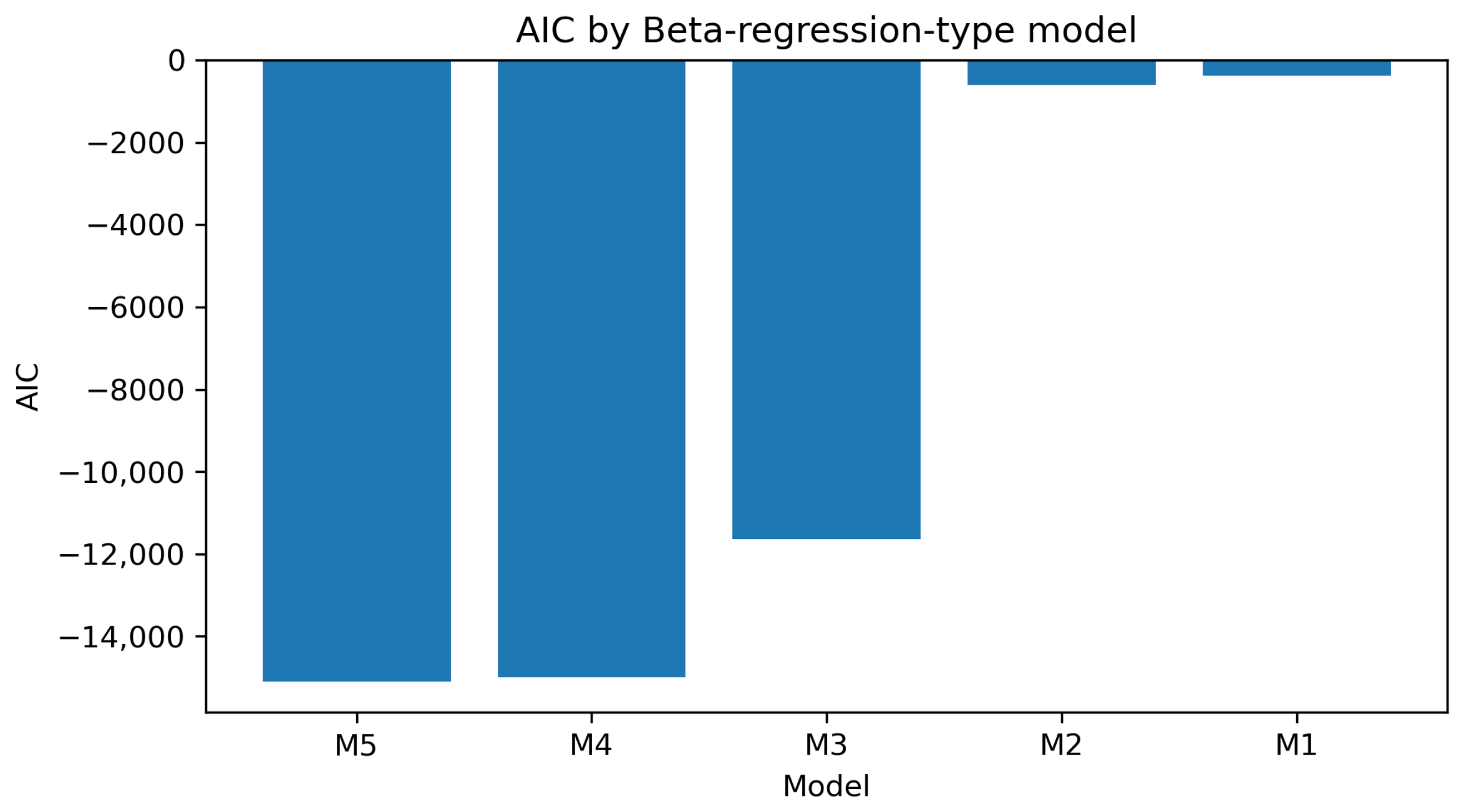
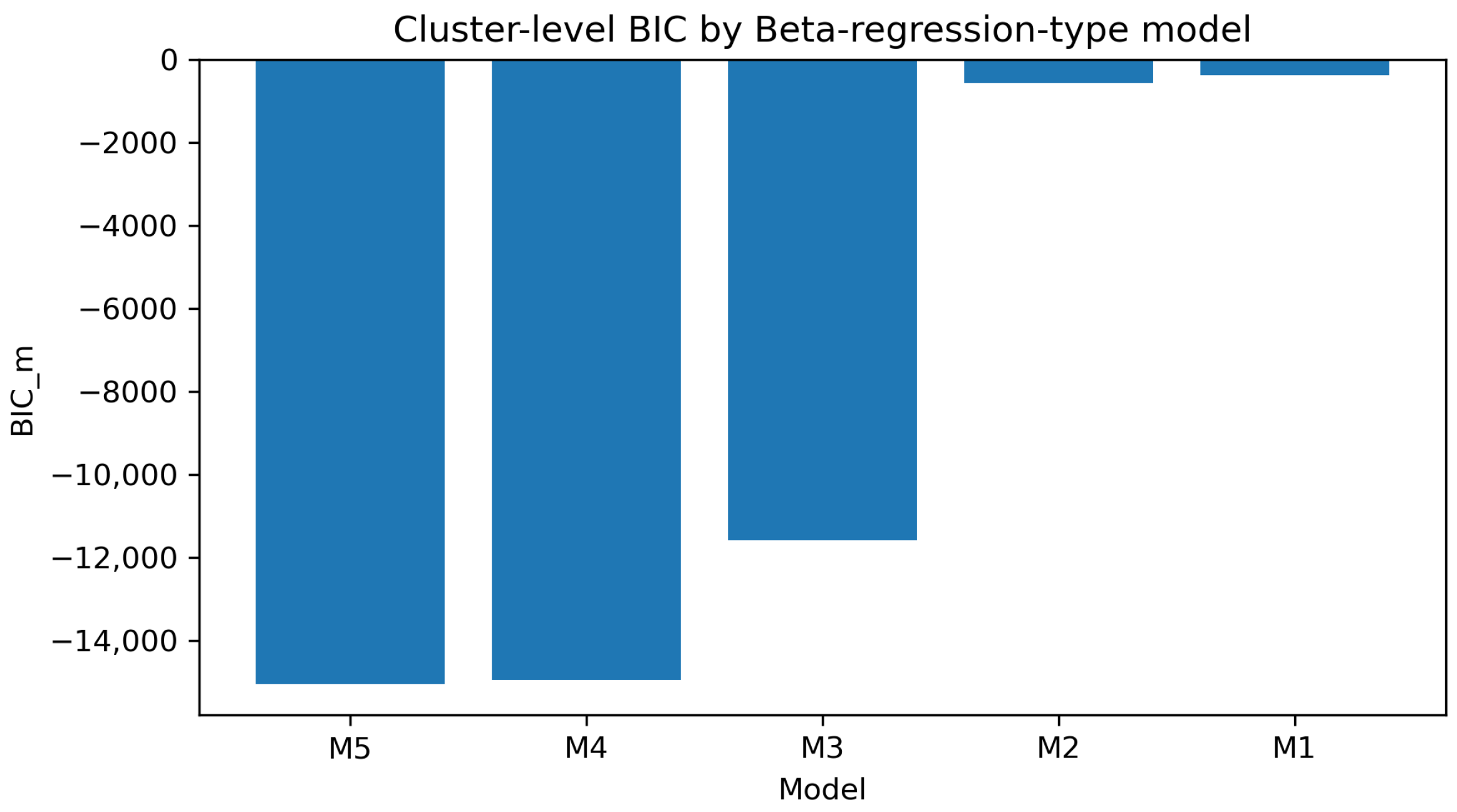
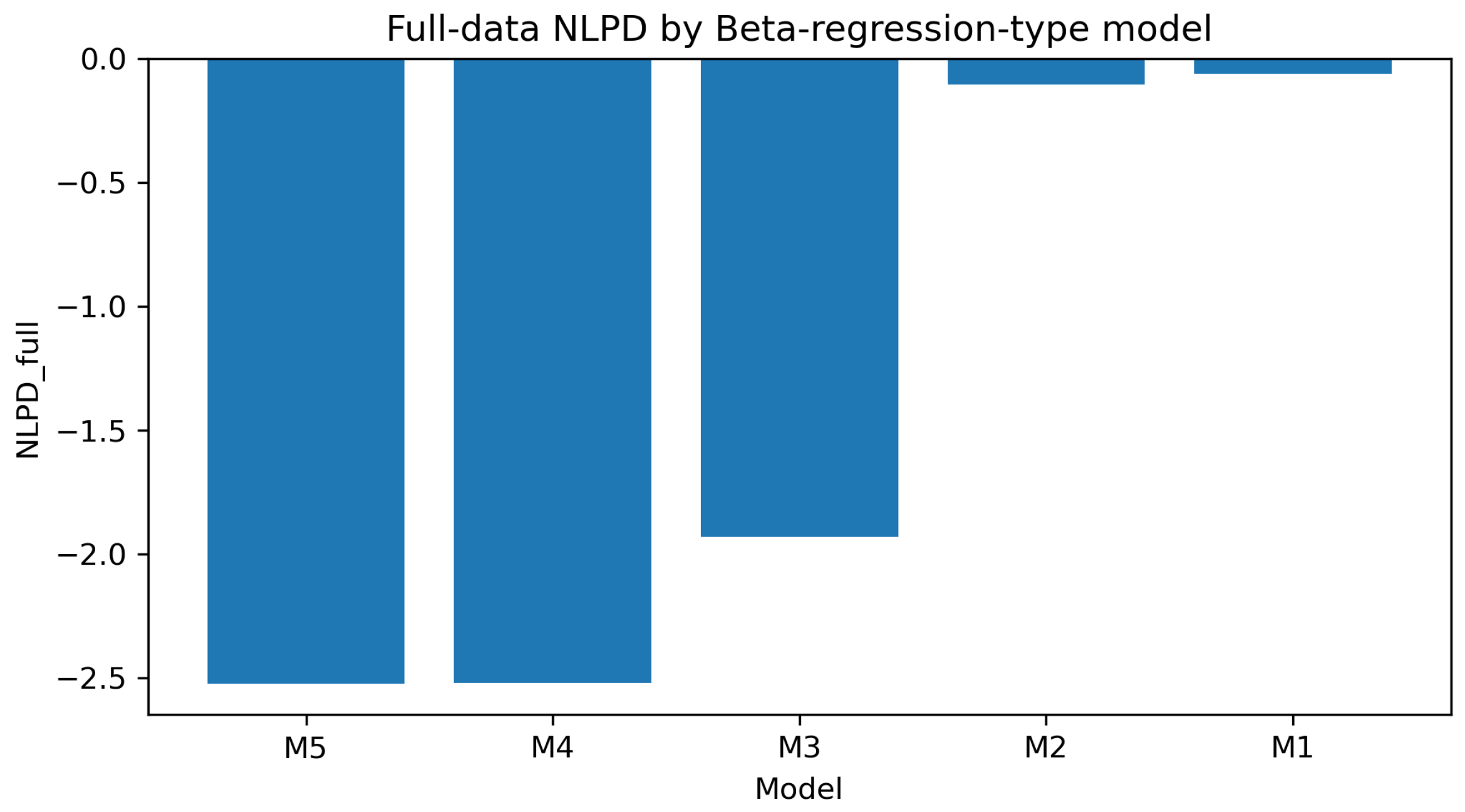
Figure 13, Figure 14 and Figure 15 visualize the same likelihood-based comparisons. In Figure 13, M5 has the smallest AIC. In Figure 14, M5 also has the smallest cluster-level BIC. Since ${\mathrm{BIC}}_m$ penalizes the additional correlation parameter more strongly than AIC, the preference for M5 under both criteria provides support for retaining the correlated random-effects structure. Figure 15 further shows that M5 achieves the best full-data distributional fit.

Because M4 is nested in M5 under the restriction $\rho =0$, we also conducted the likelihood-ratio test

$$H_0:\rho =0\mathrm{against}{H}_1:\rho \ne 0.$$

(123)

The likelihood-ratio statistic is

$$T_{\mathrm{LR}}=2\{{\widehat{\mathsf{\ell }}}_{L,\mathrm{M}5}-{\widehat{\mathsf{\ell }}}_{L,\mathrm{M}4}\}.$$

(124)

The test result is reported in

Table 17. Likelihood-ratio test comparing M5 with M4 in the real-data analysis.

Comparison	${\widehat{\mathsf{\ell }}}_{\mathit{L},\mathbf{M}4}$	${\widehat{\mathsf{\ell }}}_{\mathit{L},\mathbf{M}5}$	$\Delta {\widehat{\mathsf{\ell }}}_{\mathit{L}}$	${\mathit{T}}_{\mathbf{LR}}$	df	p-Value
M5 versus M4	7523.511	7571.151	47.640	95.280	1	$1.65\times {10}^{-22}$

. The likelihood-ratio statistic is 95.280 with $p=1.65\times {10}^{-22}$, so the null hypothesis of independent mean and precision random effects is rejected at the 5% level. The estimated correlation is $\widehat{\rho }=0.826$, indicating a strong positive latent association between adjusted state-level mean heterogeneity and adjusted state-level stability heterogeneity. Both fitted standard deviations, 2.070 and 2.229, are far from zero. Accordingly, the regular interior-point ${\chi }_1^2$ calibration is used here; the estimate is not treated as a variance-boundary case.

The finite-dimensional parameter estimates for M5 are summarized in

Table 18. Selected finite-dimensional parameter estimates under M5.

Component	Parameter	Estimate	Interpretation
Mean	${\beta }_0$	−0.118	Mean-submodel intercept
Mean	${\beta }_1$	0.034	Linear effect of standardized log adult population
Mean	${\beta }_2$	0.044	Linear mean-submodel PLACES covariate effect
Precision	${\gamma }_0$	4.773	Precision-submodel intercept
Precision	${\gamma }_1$	−0.040	Linear effect of standardized log total population
Precision	${\gamma }_2$	0.190	Linear precision-submodel PLACES covariate effect
Random effects	${\sigma }_b$	2.070	State-level mean heterogeneity
Random effects	${\sigma }_c$	2.229	State-level precision heterogeneity
Random effects	$\rho$	0.826	Mean–stability correlation

. The estimates of ${\widehat{\sigma }}_b=2.070$ and ${\widehat{\sigma }}_c=2.229$ indicate substantial state-level heterogeneity in both the mean and precision components. The positive and large value of $\widehat{\rho }$ suggests that states with higher adjusted mean levels also tend to have higher adjusted precision levels.

In this application, $\widehat{\rho }$ is the correlation between state deviations in the logit-mean and log-precision predictors after adjustment for the specified county covariates and smooth terms. It is not a correlation between raw state means and raw state variances, nor does it have a causal interpretation. Here, “stability” refers to the cross-sectional concentration of county responses around their fitted conditional means, not to stability over time. The fitted random-effect covariance is

$$\widehat{\rho }{\widehat{\sigma }}_b{\widehat{\sigma }}_c=0.826\times 2.070\times 2.229\approx 3.81.$$

Under the bivariate-normal working model, a state whose mean random effect is one fitted standard deviation above zero has expected precision random effect

$$E(c_i\mid b_i={\widehat{\sigma }}_b)=\widehat{\rho }{\widehat{\sigma }}_c\approx 1.84.$$

Holding the observed precision predictors fixed, this corresponds to an expected precision multiplier of $\exp \left(1.84\right)\approx 6.30$. This is a conditional model-scale contrast, not a directly observed or causal sixfold change.

5.4. Point-Prediction Comparison

Table 19. State-grouped holdout prediction for the CDC PLACES data. Entire states, not individual counties, were assigned to the test set. MSPE, RMSE, and MAE are smaller-is-better point-prediction criteria. The table reports one reproducible split and should not be interpreted as repeated cross-validation.

Model	Model Class	${\mathbf{MSPE}}_{\mathbf{test}}$	${\mathbf{RMSE}}_{\mathit{Y},\mathbf{test}}$	${\mathbf{MAE}}_{\mathbf{test}}$
M5	Distributional Beta model	0.00089	0.02975	0.02473
M1	Distributional Beta model	0.00090	0.03003	0.02461
M4	Distributional Beta model	0.00093	0.03056	0.02479
M3	Distributional Beta model	0.00094	0.03073	0.02492
Gradient boosting	Machine-learning benchmark	0.00098	0.03137	0.02572
Random forest	Machine-learning benchmark	0.00103	0.03207	0.02492
M2	Distributional Beta model	0.00104	0.03228	0.02655
(K)-nearest neighbors	Machine-learning benchmark	0.00118	0.03433	0.02888
Decision tree	Machine-learning benchmark	0.00136	0.03689	0.03009

reports the train/test results. M5 has the smallest test-set MSPE among the statistical and machine-learning competitors. Because the split is made by state, all counties in a held-out state remain in the test set and no cluster identifier occurs in both sets. The result therefore concerns marginal prediction for new states. M5 leads on this target and also estimates varying precision, paired state effects, and the mean–stability correlation, which are absent from M1 and the point-prediction benchmarks.

M5 also has the best AIC, ${\mathrm{BIC}}_m$, and full-data NLPD. These results, together with the lowest held-out MSPE, select it as the best overall model in the CDC analysis. It outperforms the machine-learning benchmarks in point prediction and is the only model in the comparison that provides both likelihood-based distributional inference and a state-level mean–stability interpretation.

This comparison highlights the distinction between point prediction and distributional modeling. The primary objective of the proposed model is not merely to minimize squared prediction error. Instead, M5 jointly estimates the conditional mean, conditional precision, state-level mean heterogeneity, state-level stability heterogeneity, and their latent association. Therefore, likelihood-based distributional fit and interpretability should be considered together with point-prediction accuracy.

A main advantage of the proposed model is that it produces empirical Bayes estimates ${({\widehat{b}}_i,{\widehat{c}}_i)}^{\top }$ for each state. The estimate ${\widehat{b}}_i$ measures the adjusted state-level mean effect, while ${\widehat{c}}_i$ measures the adjusted state-level precision or stability effect. Since larger precision corresponds to smaller conditional variance, larger values of ${\widehat{c}}_i$ indicate more stable county-level prevalence patterns after adjusting for observed covariates and smooth effects.

The empirical Bayes estimates ${({\widehat{b}}_i,{\widehat{c}}_i)}^{\top }$ were used to classify states into four mean–stability quadrants. The four categories are high mean–high stability, high mean–low stability, low mean–high stability, and low mean–low stability. The classification is based on centered fitted state-level mean and precision scores.

The quadrant counts are reported in

Table 20. State-level mean–stability quadrant counts under M5.

Quadrant	Number of States	Percentage
High mean–high stability	23	45.10%
High mean–low stability	2	3.92%
Low mean–high stability	2	3.92%
Low mean–low stability	24	47.06%

. Most states fall into either the high mean–high stability group or the low mean–low stability group. Specifically, 23 states are classified as high mean–high stability and 24 states are classified as low mean–low stability. Only two states are classified as high mean–low stability and two states are classified as low mean–high stability. This pattern is consistent with the large positive estimate $\widehat{\rho }=0.826$, because high fitted mean levels tend to occur together with high fitted stability.

Figure 16 shows the state-level mean–stability quadrant classification under M5. The horizontal axis represents the centered state-level fitted mean, and the vertical axis represents the centered state-level fitted precision. States in the upper-right quadrant have both higher adjusted mean levels and higher fitted stability. States in the lower-right quadrant have higher adjusted mean levels but lower fitted stability. States in the upper-left quadrant have lower adjusted mean levels but higher fitted stability. States in the lower-left quadrant have both lower adjusted mean levels and lower fitted stability [8,28].

Figure 17 maps the same quadrant classification to state locations. This geographic display provides an interpretable regional summary of the fitted state-level heterogeneity. The map shows how the proposed model can be used not only for likelihood-based inference but also for applied regional classification.

Table 21. Interpretation of the state-level mean–stability quadrants under M5.

Quadrant	Mean Effect	Stability Effect	Interpretation
High mean–high stability	${\widehat{b}}_i>0$	${\widehat{c}}_i>0$	Higher adjusted prevalence and more concentrated county-level responses
High mean–low stability	${\widehat{b}}_i>0$	${\widehat{c}}_i\le 0$	Higher adjusted prevalence but more dispersed county-level responses
Low mean–high stability	${\widehat{b}}_i\le 0$	${\widehat{c}}_i>0$	Lower adjusted prevalence with relatively stable county-level responses
Low mean–low stability	${\widehat{b}}_i\le 0$	${\widehat{c}}_i\le 0$	Lower adjusted prevalence and less stable county-level responses

summarizes the interpretation of the four quadrants. This classification is one of the main empirical outputs of the proposed framework. It cannot be obtained from M1 or M2 because they do not contain state-level random effects. It also cannot be obtained from ordinary machine-learning regressors because they do not provide a model-based precision component or a latent mean–stability association.

The county response is bounded, non-Gaussian, and heterogeneous, which supports a Beta model with a flexible precision component. The gains from M1 and M2 to M3–M5 indicate substantial state-level heterogeneity. M5 has the best AIC, ${\mathrm{BIC}}_m$, and ${\mathrm{NLPD}}_{\mathrm{full}}$, and the M5–M4 likelihood-ratio test rejects $\rho =0$. The estimate $\widehat{\rho }=0.826$ indicates a strong positive association between adjusted state-level mean and stability. M5 also has the lowest held-out MSPE and yields state rankings and quadrant classifications unavailable from the other statistical and machine-learning models. On likelihood fit, held-out point prediction, and distributional interpretation, M5 is the best overall model in the CDC analysis.

5.5. Second Application: National Renewable-Energy Consumption Shares

5.5.1. Data Source, Audit, and Model Specification

The second application uses an environmental–energy panel from the World Bank World Development Indicators (WDI), which is distinct from public-health surveillance. The response is renewable-energy consumption as a percentage of total final energy consumption (indicator EG.FEC.RNEW.ZS), divided by 100. The official indicator page is https://data.worldbank.org/indicator/EG.FEC.RNEW.ZS (accessed on 15 July 2026); it identifies the International Energy Agency as the source and gives the license as CC BY 4.0. The API snapshot was retrieved on 11 July 2026, and the API metadata list 1 July 2026 as the most recent update. Source-page metadata, direct API addresses, and SHA-256 checksums document the download.

We screened three country-level proportion panels for 2000–2022: renewable-energy consumption, forest area, and agricultural land shares. Renewable energy had the largest typical within-country variation and allowed a clear interpretation of the precision component in terms of energy-system stability. The six WDI variables were merged by ISO3 code and year, retaining complete cases. Of 3158 complete candidate country-years, 107 responses were exactly zero and none was exactly one. Eligibility required at least 18 complete years, membership in one of the four World Bank income groups, and a response strictly inside $(0,1)$ in every retained year; boundary observations were not transformed. All 128 countries meeting these prespecified rules were retained. The main analysis contains $N=2814$ observations in $m=128$ countries. Cluster sizes range from 18 to 23 (median 22), and the response has mean 0.3311, standard deviation 0.2851, median 0.2410, and range 0.001–0.983. A fixed, income-balanced sample of 24 countries is used only for sensitivity analysis.

The mean submodel contains standardized log GDP per capita at purchasing-power parity and standardized industry value added as linear terms, with urban population share fitted smoothly. The precision submodel contains standardized primary-energy intensity and standardized log per-capita energy use as linear terms, with calendar year fitted smoothly. The mean random intercept represents a persistent unobserved country deviation in renewable-energy share; the precision random intercept represents an unobserved deviation in the concentration of annual shares around their conditional means. As in the CDC analysis, we use cubic B-splines with eight basis functions, second-difference penalties, and ${\lambda }_f={\lambda }_g=1$. Standardization, min–max scaling, and spline construction are re-estimated within each prediction training set. M1–M5 retain the definitions in Table 15 for the full set of 128 eligible countries.

5.5.2. Full-Data Fitting, Correlation Inference, and Diagnostics

All five models returned finite, converged solutions. The initial M1–M5 fits took 0.01, 0.22, 290.2, 266.2, and 565.6 s, respectively, with peak process memory of approximately 224 MB on the stated machine. A fixed-$\rho$ profile supplied better nested starting values for a second optimization of M4 and M5 under the same sample, model, and objective. These two fits took a further 46.3 and 46.7 s.

Table 22. M1–M5 full-data comparison for all 128 eligible World Bank countries. M5 has the largest marginal log-likelihood and the smallest AIC and cluster-level ${\mathrm{BIC}}_m$; bold marks these results and its estimated correlation. NLPD and fitted RMSE are reported as secondary descriptive checks.

Model	${\widehat{\mathsf{\ell }}}_{\mathit{L}}$	AIC	${\mathbf{BIC}}_{\mathit{m}}$	NLPD	Fitted RMSE	$\widehat{\mathit{\rho }}$
M1	1375.266	−2742.532	−2731.124	−0.489	0.1988	–
M2	1687.703	−3331.406	−3268.661	−0.600	0.1932	–
M3	5491.350	−10,936.701	−10,871.104	−2.135	0.0395	–
M4	6056.262	−12,064.524	−11,996.075	−2.436	0.0400	0.000
M5	6064.947	−12,079.894	−12,008.593	−2.435	0.0401	−0.500

favors M5 on the full-data likelihood criteria: relative to refined M4, M5 raises the marginal log-likelihood by 8.685 and lowers AIC and cluster-level BIC by 15.370 and 12.518. The significant M4–M5 likelihood-ratio test leads to the same selection, making M5 the best overall full-data model. Full-data NLPD is nearly tied and favors M4 by 0.0004 ($-2.4355$ versus $-2.4352$); fitted RMSE values are also similar across M3–M5. These measures are reported because they assess aspects of fit other than the likelihood-based selection criteria.

Under M5, ${\widehat{\sigma }}_b=1.984$, ${\widehat{\sigma }}_c=1.526$, and $\widehat{\rho }=-0.500$. After adjustment, countries with persistently higher renewable-energy shares therefore tend to have lower conditional precision and greater annual dispersion around their conditional means. The M4–M5 likelihood-ratio statistic is 17.370 ($p=3.08\times {10}^{-5}$), which rejects independence. A fixed-$\rho$ profile gives an interpolated 95% likelihood-ratio interval of $(-0.621,-0.295)$ and is used in place of the unstable generic quasi-Newton Wald interval. In contrast to the positive CDC estimate, the World Bank estimate is negative; M5 allows the data in each domain to determine the direction of the mean–stability association.

Figure 18 shows the response, cluster sizes, and model-consistent M5 diagnostics. The conditional quantile residuals have mean $-0.013$, standard deviation 0.982, and range $-2.836$ to 3.287; only two of 2814 residuals exceed 3 in absolute value. The PIT mean is 0.495. The uniform-PIT test rejects exact calibration ($p=5.39\times {10}^{-10}$), and the Q–Q plot has visible tail curvature, so the fitted distribution is not perfectly calibrated. A prespecified screen combining cluster residual magnitude with empirical Bayes effect magnitude identifies Moldova, Gabon, and Algeria. When all three are removed, M5 still lowers AIC by 9.100 relative to M4, and the nested test remains significant (LR $=11.100$, $p=8.63\times {10}^{-4}$). The refitted correlation decreases to $-0.119$. Its magnitude is therefore sensitive to these countries, but the likelihood-based preference for M5 is unchanged.

5.5.3. Repeated Grouped Prediction and Cross-Domain Comparison

The primary prediction target is the renewable-energy share in future years for countries observed during training. Across the three fixed rolling origins (2016, 2018, and 2020), M5 has the lowest mean MSPE (0.003767), RMSE (0.061205), and MAE (0.045656), making it the best point-prediction model for this target.

Table 23. World Bank prediction comparison. The application-aligned primary target is point prediction of future years for countries observed during training; means (standard errors) are reported across the fixed 2016, 2018, and 2020 rolling origins, and M5 is best for MSPE, RMSE, and MAE (bold). Future-year NLPD and the unchanged two-by-three-fold new-country RMSE are retained as secondary density and transportability audits.

Model	Future-Year MSPE	Future-Year RMSE	Future-Year MAE	Future-Year NLPD	New-Country RMSE
M1	0.039940 (0.000124)	0.199850 (0.000310)	0.153573 (0.000411)	−0.359 (0.009)	0.1934 (0.0179)
M2	0.038866 (0.000112)	0.197144 (0.000284)	0.149765 (0.000327)	−0.481 (0.005)	0.2258 (0.0125)
M3	0.003812 (0.000430)	0.061537 (0.003580)	0.045950 (0.002766)	−1.434 (0.081)	0.2224 (0.0186)
M4	0.003771 (0.000375)	0.061251 (0.003126)	0.045669 (0.002394)	−1.304 (0.289)	0.2222 (0.0190)
M5	0.003767 (0.000385)	0.061205 (0.003206)	0.045656 (0.002458)	−1.261 (0.325)	0.2227 (0.0155)

also reports variation across origins. Two additional analyses address different targets. M3 has the lowest mean future-year NLPD ($-1.434$ versus $-1.261$ for M5). In the fixed income-balanced sample of 24 countries, the two-by-three-fold grouped analysis gives M1 the lowest RMSE (0.1934) when every test country is unseen and no country effect can be estimated for it. The first comparison concerns density calibration and the second concerns marginal transportability to new countries.

Figure 19 summarizes the full-data likelihood comparison and the M5 country effects.

Table 24. Cross-domain comparison under the common M1–M5 hierarchy. In both applications, AIC, cluster-level ${\mathrm{BIC}}_m$, the nested M4–M5 test, and the application-specific point-prediction target select M5. Bold identifies the model selected by each primary criterion and the overall primary decision. This combined evidence identifies M5 as the best overall model in both domains. Table 22 and Table 23 separately report density and transportability results for different targets.

Data	N	m	AIC Winner	${\mathbf{BIC}}_{\mathit{m}}$ Winner	M4–M5 LR $\left(\mathit{p}\right)$	Primary Prediction Winner	${\widehat{\mathit{\rho }}}_{\mathit{M}5}$	Primary Decision
CDC PLACES	3143	51	M5	M5	95.280 ($1.65\times {10}^{-22}$)	M5	0.826	M5
World Bank WDI	2814	128	M5	M5	17.370 ($3.08\times {10}^{-5}$)	M5	−0.500	M5

places the two applications on the same likelihood, dependence-testing, and application-specific prediction criteria. In both CDC PLACES and WDI, M5 has the best AIC and cluster-level BIC, rejects the independent-effects restriction in M4, and has the lowest point-prediction errors for the stated target. It is therefore the best overall model in both applications. The strongly positive $\widehat{\rho }$ in CDC and the significantly negative estimate in WDI show that the direction of mean–stability dependence is determined by the application rather than imposed by M5. Table 22 and Table 23 also report density and unseen-country results; model rankings can differ for these distinct scoring rules and information sets.

The World Bank analysis has several limitations. Inclusion of all 128 eligible countries does not make the complete-case, open-interval panel globally representative. WDI measurements may contain country-specific reporting errors, and the model does not include serial or spatial correlation beyond the country effects. The balanced-sample new-country analysis has six splits, whereas rolling-origin prediction concerns countries observed during training; the two targets are not interchangeable. Coefficients and country effects are associational rather than causal. Within the observed panel and the stated prediction target, AIC, cluster-level BIC, the nested dependence test, and all three rolling-origin point-error criteria select M5.

6. Conclusions and Discussion

This paper introduces a correlated mean–precision random-effects Beta regression model for clustered proportion data. Its main methodological contribution is to treat $\rho =\mathrm{Corr}(b_i,c_i)$ as a primary estimand within a model that also allows semiparametric adjustment, likelihood-based testing, prediction, and empirical Bayes cluster interpretation. Mean and precision heterogeneity are therefore estimated jointly, with direct inference on their latent cluster-level association.

The proposed model includes several commonly used Beta regression-type models as reduced cases, including constant-precision Beta regression, varying-precision Beta regression, mean-only random-effects Beta regression, and independent mean–precision random-effects Beta regression. Estimation is carried out by maximizing a penalized marginal likelihood based on a Laplace approximation. The transformations ${\sigma }_b=\exp \left({\omega }_b\right)$, ${\sigma }_c=\exp \left({\omega }_c\right)$, and $\rho =\tanh \left(\xi \right)$ ensure valid variance components and correlation during optimization. The fitted model provides estimates of the fixed effects, smooth effects, variance components, the mean–stability correlation, and empirical Bayes estimates of the cluster-level random effects.

The simulation results select M5 as the best overall model for the objectives considered. Among M1–M5, it has the best average recovery of both the conditional mean and precision and the best average AIC, BIC_m, and full-data NLPD. Its new-cluster point prediction remains in the leading group when $\rho$ is weak or zero, with further gains in recovery and fit when mean and precision heterogeneity are correlated. The likelihood-ratio test has high empirical power under strong positive or negative correlations and appropriate type-I-error behavior under $\rho =0$. M5 alone combines this performance with direct inference on $\rho$ and paired cluster-level mean–stability interpretation.

The enlarged stress suite shows where this conclusion becomes harder to support. All 300 nonnull M5 fits succeeded, and every aggregate mean criterion favored M5 across 299 successful M4–M5 pairs. The relative recovery differences were $-2.188\%$ for ${\mathrm{RMSE}}_{\mu }$ and $-2.550\%$ for ${\mathrm{RMSE}}_{\varphi }$; the AIC, BIC_m, and full-data NLPD differences were also negative. In the extreme response-near-zero and near-zero-${\sigma }_c$ settings, information about the correlation is weak and boundary-aware diagnostics and bootstrap calibration are needed. At the fitted parameter values checked, AGHQ was stable and closely matched the Laplace approximation.

Both applications select M5 as the best overall model when likelihood, application-aligned prediction, and inferential scope are considered jointly. In CDC PLACES, M5 has the best AIC, cluster-level BIC, and full-data NLPD, rejects the independent-effects M4 restriction, achieves the lowest grouped-holdout MSPE and RMSE, and identifies a strong positive latent mean–stability association. In the representative World Bank panel of all 128 eligible countries, M5 again has the best AIC and ${\mathrm{BIC}}_m$, rejects M4, and has the lowest rolling-origin MSPE, RMSE, and MAE, while identifying a significant negative association between adjusted renewable-energy level and conditional stability. The opposite correlation signs show the interpretive value of estimating the dependence rather than assuming a common direction across domains.

Future work may extend the proposed framework in several directions. Zero–one-inflated models could handle boundary responses. Robust or mixture random-effects distributions could improve performance under nonnormal cluster heterogeneity. Spatially correlated random effects would be useful for regional proportion data. Bayesian versions could provide full posterior uncertainty for $\rho$, cluster rankings, and quadrant membership. Extensions to longitudinal clustered proportions and multivariate proportion responses are also promising [30].

The bivariate normal is the working distribution for the random effects, while the stress study also considers selected heavy-tailed and contaminated alternatives. Remark 1 and the boundary experiments identify small variance components and few independent clusters as conditions requiring additional diagnostic care. The AGHQ results support the two-dimensional Laplace calculation at the fitted values examined; higher-order quadrature may be useful under more difficult curvature. The CDC and WDI analyses illustrate the same workflow in two domains.

Further work could extend the empirical and computational evaluation. For CDC PLACES, model-consistent conditional quantile, PIT, and Pearson residuals could be combined with leave-one-state-out refits. The current CDC analysis instead uses likelihood comparisons and one state-grouped holdout. Repeated nested state-grouped cross-validation would measure how stable the CDC rankings are across partitions. Because the present implementation fixes $p=q=3$, high-dimensional covariates would require a regularized estimator with variable selection and tuning within each training fold. A matched Bayesian comparison would also need prespecified priors, samplers, convergence criteria, posterior diagnostics, and sensitivity analyses before uncertainty and computing cost could be compared with M5.

M5 jointly models average level and conditional stability, tests their latent cluster-level association, and uses the paired random effects for cluster interpretation. It has the strongest combined performance among M1–M5 in the main simulation and the enlarged stress suite. Likelihood, application-specific prediction, and correlation inference also select M5 as the best overall model in both CDC PLACES and the representative World Bank panel. The estimated association is strongly positive in the public-health application and significantly negative in the environmental–energy application. Among the models and settings evaluated here, M5 provides the best overall combination of fit, prediction, and scientific interpretation.

References

1. Ferrari, S.; Cribari-Neto, F. Beta regression for modelling rates and proportions. J. Appl. Stat. 2004, 31, 799–815. [Google Scholar] [CrossRef]
2. Cribari-Neto, F.; Zeileis, A. Beta Regression in R. J. Stat. Softw. 2010, 34, 1–24. [Google Scholar] [CrossRef]
3. Geissinger, E.A.; Khoo, C.L.L.; Richmond, I.C.; Faulkner, S.J.M.; Schneider, D.C. A case for beta regression in the natural sciences. Ecosphere 2022, 13, e3940. [Google Scholar] [CrossRef]
4. Cribari-Neto, F.; e Silva, J.J.S.; Vasconcellos, K.L.P. Beta regression misspecification tests. J. Stat. Plan. Inference 2024, 233, 106193. [Google Scholar] [CrossRef]
5. Bourguignon, M.; Gallardo, D.I. A general and unified parameterization of the beta distribution: A flexible and robust beta regression model. Stat. Neerl. 2025, 79, e70007. [Google Scholar] [CrossRef]
6. Breslow, N.E.; Clayton, D.G. Approximate Inference in Generalized Linear Mixed Models. J. Am. Stat. Assoc. 1993, 88, 9–25. [Google Scholar] [CrossRef]
7. Pinheiro, J.C.; Bates, D.M. Approximations to the Log-Likelihood Function in the Nonlinear Mixed-Effects Model. J. Comput. Graph. Stat. 1995, 4, 12–35. [Google Scholar] [CrossRef]
8. Ning, X.; Hui, F.K.C.; Welsh, A. Inferential procedures for random effects in generalized linear mixed models. PLoS ONE 2025, 20, e0320797. [Google Scholar] [CrossRef] [PubMed]
9. Rigby, R.A.; Stasinopoulos, D.M. Generalized additive models for location, scale and shape. J. R. Stat. Soc. Ser. C Appl. Stat. 2005, 54, 507–554. [Google Scholar] [CrossRef]
10. Heller, G.Z.; Robledo, K.P.; Marschner, I.C. Distributional regression in clinical trials: Treatment effects on parameters other than the mean. BMC Med. Res. Methodol. 2022, 22, 56. [Google Scholar] [CrossRef] [PubMed]
11. Klein, N. Distributional Regression for Data Analysis. Annu. Rev. Stat. Its Appl. 2024, 11, 321–346. [Google Scholar] [CrossRef]
12. Marx, B.D.; Eilers, P.H.C. Generalized Linear Regression on Sampled Signals and Curves: A P-Spline Approach. Technometrics 1999, 41, 1–13. [Google Scholar] [CrossRef]
13. Hastie, T.J.; Tibshirani, R.J. Generalized Additive Models. Stat. Sci. 1986, 1, 297–310. [Google Scholar] [CrossRef]
14. Bak, K.Y.; Lee, D.Y.; Lee, J.S.; Jee, H.J.; Park, R.J.; Koo, J.Y.; Jhong, J.H. Efficient curve fitting with penalized B-splines for oceanographic and ecological applications. Sci. Rep. 2025, 15, 21958. [Google Scholar] [CrossRef] [PubMed]
15. Figueroa-Zúñiga, J.I.; Arellano-Valle, R.B.; Ferrari, S.L.P. Mixed Beta Regression: A Bayesian Perspective. Comput. Stat. Data Anal. 2013, 61, 137–147. [Google Scholar] [CrossRef]
16. Tang, B.; Frye, H.A.; Gelfand, A.E.; Silander, J.A. Zero-Inflated Beta Distribution Regression Modeling. J. Agric. Biol. Environ. Stat. 2023, 28, 117–137. [Google Scholar] [CrossRef]
17. Ospina, R.; Ferrari, S.L.P. A general class of zero-or-one inflated beta regression models. Comput. Stat. Data Anal. 2012, 56, 1609–1623. [Google Scholar] [CrossRef]
18. Kneib, T.; Silbersdorff, A.; Säfken, B. Rage Against the Mean—A Review of Distributional Regression Approaches. Econom. Stat. 2023, 26, 99–123. [Google Scholar] [CrossRef]
19. Acharyya, S.; Pati, D.; Sun, S.; Bandyopadhyay, D. A monotone single index model for missing-at-random longitudinal proportion data. J. Appl. Stat. 2024, 51, 1023–1040. [Google Scholar] [CrossRef] [PubMed]
20. da Paz, R.; Bazán, J.L.; Lachos, V.H.; Dey, D. A finite mixture mixed proportion regression model for classification problems in longitudinal voting data. J. Appl. Stat. 2023, 50, 871–888. [Google Scholar] [CrossRef] [PubMed]
21. Umlauf, N.; Klein, N.; Simon, T.; Zeileis, A. bamlss: A Lego Toolbox for Flexible Bayesian Regression (and Beyond). J. Stat. Softw. 2021, 100, 1–53. [Google Scholar] [CrossRef]
22. Rügamer, D.; Kolb, C.; Klein, N. Semi-Structured Distributional Regression. Am. Stat. 2024, 78, 88–99. [Google Scholar] [CrossRef]
23. Da Silva, G.P.; Laureano, H.A.; Petterle, R.R.; Ribeiro, P.J.; Bonat, W.H. Multivariate generalized linear mixed models for underdispersed count data. J. Stat. Comput. Simul. 2023, 93, 2410–2427. [Google Scholar] [CrossRef]
24. Siegfried, S.; Kook, L.; Hothorn, T. Distribution-Free Location-Scale Regression. Am. Stat. 2023, 77, 345–356. [Google Scholar] [CrossRef]
25. Liu, T.; Ding, B. A radial basis function neural network approach for solving a diffusion partial differential equation efficiently. Appl. Math. Comput. 2026, 509, 129651. [Google Scholar] [CrossRef]
26. Liu, Y.; Li, Y.; Liu, T. An RBF–FD method for pricing under the Bates model: Handling stochastic volatility and jump processes. Eng. Anal. Bound. Elem. 2026, 183, 106622. [Google Scholar] [CrossRef]
27. Joe, H. Accuracy of Laplace approximation for discrete response mixed models. Comput. Stat. Data Anal. 2008, 52, 5066–5074. [Google Scholar] [CrossRef]
28. Rainey, M.J.; Keller, K.P. Semiparametric Approaches for Mitigating Spatial Confounding in Large Environmental Epidemiology Cohort Studies. Environmetrics 2025, 36, e70028. [Google Scholar] [CrossRef] [PubMed]
29. Ver Hoef, J.M.; Blagg, E.; Dumelle, M.; Dixon, P.M.; Zimmerman, D.L.; Conn, P.B. Marginal inference for hierarchical generalized linear mixed models with patterned covariance matrices using the Laplace approximation. Environmetrics 2024, 35, e2872. [Google Scholar] [CrossRef] [PubMed]
30. Kock, L.; Klein, N. Truly Multivariate Structured Additive Distributional Regression. J. Comput. Graph. Stat. 2025, 34, 1189–1201. [Google Scholar] [CrossRef]
31. Benavidez, G.A.; Zahnd, W.E.; Hung, P.; Eberth, J.M. Chronic Disease Prevalence in the US: Sociodemographic and Geographic Variations by Zip Code Tabulation Area. Prev. Chronic Dis. 2024, 21, 230267. [Google Scholar] [CrossRef] [PubMed]
32. Kosmidis, I.; Zeileis, A. Extended-support beta regression for [0, 1] responses. J. R. Stat. Soc. Ser. C Appl. Stat. 2026, 75, 139–157. [Google Scholar] [CrossRef]
33. Baey, C.; Kuhn, E. varTestnlme: An R Package for Variance Components Testing in Linear and Nonlinear Mixed-Effects Models. J. Stat. Softw. 2023, 107, 1–32. [Google Scholar] [CrossRef]
34. Ekvall, K.O.; Bottai, M. Confidence regions near singular information and boundary points with applications to mixed models. Ann. Stat. 2022, 50, 1806–1832. [Google Scholar] [CrossRef]
35. Andersson, B.; Jin, S.; Zhang, M. Fast Estimation of Multiple Group Generalized Linear Latent Variable Models for Categorical Observed Variables. Comput. Stat. Data Anal. 2023, 182, 107710. [Google Scholar] [CrossRef]
36. Mamun, A.; Paul, S. Model Selection in Generalized Linear Models. Symmetry 2023, 15, 1905. [Google Scholar] [CrossRef]
37. Abo El Nasr, M.M.; Abdelmegaly, A.A.; Abdo, D.A. Performance Evaluation of Different Regression Models: Application in a Breast Cancer Patient Data. Sci. Rep. 2024, 14, 12986. [Google Scholar] [CrossRef] [PubMed]
38. Xu, S.; Ferreira, M.A.R.; Porter, E.M.; Franck, C.T. Bayesian model selection for generalized linear mixed models. Biometrics 2023, 79, 3266–3278. [Google Scholar] [CrossRef] [PubMed]
39. Hodson, T.O. Root-Mean-Square Error (RMSE) or Mean Absolute Error (MAE): When to Use Them or Not. Geosci. Model Dev. 2022, 15, 5481–5487. [Google Scholar] [CrossRef]
40. Allen, S. Weighted scoringRules: Emphasizing Particular Outcomes When Evaluating Probabilistic Forecasts. J. Stat. Softw. 2024, 110, 1–26. [Google Scholar] [CrossRef]
41. Cevid, D.; Michel, L.; Näf, J.; Bühlmann, P.; Meinshausen, N. Distributional Random Forests: Heterogeneity Adjustment and Multivariate Distributional Regression. J. Mach. Learn. Res. 2022, 23, 1–79. [Google Scholar]
42. Klein, N.; Nott, D.J.; Smith, M.S. Marginally Calibrated Deep Distributional Regression. J. Comput. Graph. Stat. 2021, 30, 467–483. [Google Scholar] [CrossRef]
43. Gao, P.A.; Wakefield, J. A Spatial Variance-Smoothing Area Level Model for Small Area Estimation of Demographic Rates. Int. Stat. Rev. 2023, 91, 493–510. [Google Scholar] [CrossRef] [PubMed]
Figure 1. Workflow for the correlated mean–precision random-effects Beta regression. The two distributional predictors share paired cluster-level random effects. Laplace’s method approximates the two-dimensional cluster integrals before global parameter optimization and inference.
Axioms 15 00576 g001
Figure 2. Conditional-mean recovery for M1–M5 across the 23 settings in Section 4.1, each repeated 50 times. Bar height is the average RMSE μ over settings and replications. The response is evaluated on its probability scale, and smaller values indicate better recovery. Model definitions are given in Table 2.
Axioms 15 00576 g002
Figure 3. Conditional-precision recovery for M1–M5 across the 23 settings in Section 4.1, each repeated 50 times. Bar height is the average RMSE ϕ over settings and replications on the precision scale. Smaller values indicate better recovery; model definitions are given in Table 2.
Axioms 15 00576 g003
Figure 4. Full-data negative logarithmic score for M1–M5 across the 23 settings in Section 4.1, each repeated 50 times. Bar height is the average NLPDfull over settings and replications. This is an in-sample conditional-density score rather than a held-out prediction score. Smaller values, including more negative values for continuous densities, indicate better fit.
Axioms 15 00576 g004
Figure 5. Sampling distribution of ρ ^ from M5 in the five baseline correlation settings ( m = 100 , n i = 10 , 50 replications each). The horizontal axis gives the generating value and the vertical axis gives the estimate. Each box shows the median and interquartile range; whiskers extend to the conventional 1.5 interquartile-range limits and points beyond them are displayed individually.
Axioms 15 00576 g005
Figure 6. Empirical rejection rate of the M5-versus-M4 likelihood-ratio test across 50 replications at each generating value of ρ . The dashed horizontal line is the nominal 5% level. The corresponding Wilson intervals are reported in Table 4; uncertainty is widest for rejection rates near one half.
Axioms 15 00576 g006
Figure 7. Paired M5-minus-M4 AIC differences over the simulation settings and replications for which both models were fitted. The vertical reference is zero. Negative values favor M5, while positive values favor the nested independent-effects model M4 after the AIC penalty.
Axioms 15 00576 g007
Figure 8. Paired M5-minus-M4 cluster-level BIC m differences over the simulation settings and replications. Negative values favor M5; positive values favor M4 under the stronger cluster-level penalty for the additional correlation parameter.
Axioms 15 00576 g008
Figure 9. Paired M5-minus-M4 differences in RMSE ϕ over the simulation settings and replications. The vertical reference is zero, and negative values indicate more accurate conditional-precision recovery by M5.
Axioms 15 00576 g009
Figure 10. Paired M5-minus-M4 differences in the full-data negative logarithmic score. Negative values favor M5. The score is conditional and in-sample; it is distinct from the held-out NLPDtest.
Axioms 15 00576 g010
Figure 11. Paired M5-minus-M4 differences in test-set MSPE for new clusters. Negative values favor M5 and positive values favor M4. The differences concentrate near zero; M5 therefore retains M4’s point-prediction accuracy while adding correlation inference, joint distributional recovery, and paired cluster interpretation.
Axioms 15 00576 g011
Figure 12. Paired M5-minus-M4 comparisons in the enlarged nonnull stress suite. Points are scenario-specific means and bars are ± 1.96 Monte Carlo standard errors; only replications in which both models succeeded are included. Negative values favor M5. Recovery panels use paired relative changes to compare low- and high-precision settings on the same scale. The final panel gives the fraction of all 299 successful pairs favoring M5; the dashed line is 0.5. Red marks settings or aggregate criteria that favor M5, whereas gray marks those that favor M4. Every setting is displayed, including those that favor M4.
Axioms 15 00576 g012
Figure 13. AIC for M1–M5 fitted to 3143 counties in 51 state-level clusters. Values use the unpenalized Laplace-approximated marginal log-likelihood evaluated at the penalized estimates and the common working parameter-count rule. Smaller values indicate better fit; M5 has the smallest AIC.
Axioms 15 00576 g013
Figure 14. Cluster-level BIC m for M1–M5 in the CDC PLACES analysis, with m = 51 independent state-level clusters. Smaller values indicate better fit after the cluster-level Schwarz penalty. M5 has the smallest BIC m despite the stronger penalty for model complexity.
Axioms 15 00576 g014
Figure 15. Full-data negative logarithmic score for M1–M5 over 3143 counties. The score evaluates each fitted conditional Beta density and is in-sample, not cross-validated. Smaller values, including more negative values, indicate better distributional fit; M5 gives the smallest value.
Axioms 15 00576 g015
Figure 16. State-level empirical Bayes mean–stability scores under M5 for the 50 states and the District of Columbia. The coordinates are centered fitted mean and precision summaries, and dashed lines define the four descriptive quadrants. Points near either line should not be treated as having certain membership because posterior classification probabilities are not displayed.
Axioms 15 00576 g016
Figure 17. Geographical display of the descriptive M5 empirical Bayes quadrant assignments. Colors encode the four adjusted mean–stability groups. The map summarizes cross-sectional county concentration and does not represent temporal stability or causal effects.
Axioms 15 00576 g017
Figure 18. World Bank renewable-energy data and M5 diagnostics for all 128 eligible countries. (a) The response is a natural proportion and is not boundary transformed. (b) Each country contributes 18–23 annual observations. (c) Continuous conditional Beta quantile residuals use the fitted M5 μ ^ and ϕ ^ . (d) Residuals versus fitted means are colored by log fitted precision. Panels (c,d) display the observed tail and PIT departures.
Axioms 15 00576 g018
Figure 19. Model comparison and country effects in the representative World Bank application. Panels (a,b) show AIC and cluster-level BIC differences from the best model; M5 is best for both. Panel (c) shows M5’s marginal log-likelihood gain over nested M4 and the likelihood-ratio result. Panel (d) displays M5 empirical-Bayes country effects; labels mark the seven largest bivariate magnitudes.
Axioms 15 00576 g019