On the Structural Distortion Induced by the Inverse Box–Cox Transformation

Abstract

The Box–Cox transformation is widely used to improve normality, stabilize variance, and enable Gaussian-based modelling in a transformed scale. After model fitting, conditional summaries are often mapped back to the original scale by applying the inverse transformation. This paper shows that this transform–fit–inverse procedure has a structural limitation: nonlinear inverse transformations do not, in general, preserve conditional expectations. Equivalently, conditional expectation and nonlinear inversion do not commute. Within the Box–Cox Gaussian framework, the admissible domain of the inverse transformation leads naturally to a truncated normal formulation in the transformed scale. Under this formulation, we derive a second-order decomposition showing that the original-scale conditional mean differs from the inverse-transformed truncated conditional mean by a curvature-driven correction term depending on the truncated conditional variance. The usual untruncated Gaussian expression is recovered as a local approximation when the inadmissible probability is negligible. A numerical sensitivity analysis, focused on $0\le {\lambda }_Y\le 1$, illustrates how the distortion depends on the transformation parameter, correlation, and conditional dispersion. A real-data illustration using medical insurance charges further shows that the discrepancy can be visible in an applied regression setting and is not removed by changing the transformation of the explanatory variable. The results distinguish this structural invariance problem from classical retransformation bias and show that inverse-transformed fitted curves should be interpreted as transformation-induced structural curves, not automatically as conditional mean functions on the original scale.

1. Introduction

Transformation-based modelling is a standard strategy in statistics. A nonlinear transformation is often applied to the response variable, or to several variables, in order to improve normality, stabilize variance, or simplify the dependence structure. After fitting a model in the transformed scale, fitted values, regression curves, or conditional summaries are commonly mapped back to the original scale by applying the inverse transformation. This transform–fit–inverse procedure is natural and widely used, but it raises a fundamental question: which statistical structures are preserved when a model fitted in the transformed scale is returned to the original scale?

This question is particularly important for conditional expectations. In regression analysis, the conditional mean is often the primary object of interpretation and prediction. However, conditional expectation is a linear operator, whereas the inverse of a nonlinear transformation is itself nonlinear. As a consequence, the inverse transformation of a conditional mean in the transformed scale does not generally coincide with the conditional mean in the original scale. In operator terms, nonlinear transformations do not commute with conditional expectation.

The Box–Cox transformation, introduced by [1], provides a classical and analytically tractable setting in which this issue can be studied. It is widely used for variance stabilization, improvement of normality, and simplification of functional relationships in statistical modelling [2,3,4]. It is also closely related to the Power Normal distribution family introduced by [5], which provides a probabilistic framework for transformation-based Gaussian modelling [6,7,8]. The transformation continues to be used in modern applications, including data-driven modelling and machine-learning contexts [9,10].

The phenomenon studied here is related to, but distinct from, the classical retransformation bias problem. Retransformation bias is primarily concerned with corrected prediction or mean estimation on the original scale after fitting a model in a transformed scale [11,12,13,14,15]. In contrast, the present paper addresses a structural invariance question: whether the conditional mean operator itself is preserved by a transform–fit–inverse modelling pipeline.

The contribution of this paper is to make explicit this structural non-commutativity principle in the Box–Cox framework. If h is a nonlinear inverse transformation and V is a transformed response, then in general

$$\mathbb{E}\left[h\right(V)\mid U]\ne h\left\{\mathbb{E}\right[V\mid U\left]\right\}.$$

Equality can hold under restrictive conditions, such as affine transformations or degenerate conditional distributions, but it is not a generic property of nonlinear transformation-based models. Thus, the inverse image of a conditional mean in the transformed scale is generally a structural curve induced by the transformation, not the conditional mean function in the original scale.

Within the Box–Cox setting, the admissible-domain issue must also be taken into account. The inverse Box–Cox map is defined only on

$${\mathcal{D}}_{\lambda }=\{u\in \mathbb{R}:1+\lambda u>0\}.$$

Thus, an unrestricted Gaussian latent variable is not globally compatible with the inverse Box–Cox map whenever $\lambda \ne 0$. For this reason, the exact probabilistic formulation considered in this paper is based on the Gaussian density restricted to the admissible domain, that is, on a truncated normal formulation in the transformed scale. In that formulation, the discrepancy between the original-scale conditional mean and the inverse-transformed conditional mean is governed, to second order, by the curvature of the inverse transformation and by the conditional variance in the transformed domain.

Transformation methods have a long history in statistical modelling and have been used not only to improve approximate normality, but also to reduce skewness, stabilize variance and simplify regression [1,16]. The Box–Cox transformation is one of the most widely used members of this tradition, but it is part of a broader class of transformation-based methods, including later extensions such as the Yeo–Johnson transformation for variables that may take nonpositive values [17]. Multivariate versions of the Box–Cox transformation have also been proposed in order to address joint normality and dependence structure [18].

Related transformation ideas also appear in Gaussian copula modelling and in modern statistical learning procedures, where nonlinear marginal transformations are often used to separate marginal behaviour from dependence modelling. The present paper focuses on a different, but related, issue: the effect of nonlinear inverse transformations on conditional means after fitting a model in the transformed scale.

The transform–fit–invert pipeline considered in this paper can be summarized schematically as

$$(X,Y)⟶(U,V)=\{g_{{\lambda }_X}\left(X\right),g_{{\lambda }_Y}\left(Y\right)\}⟶\mathbb{E}[V\mid U=u]⟶g_{{\lambda }_Y}^{-1}\left\{\mathbb{E}[V\mid U=u]\right\}.$$

The structural discrepancy arises in the final step because

$$g_{{\lambda }_Y}^{-1}\left\{\mathbb{E}[V\mid U=u]\right\}\ne \mathbb{E}\{g_{{\lambda }_Y}^{-1}\left(V\right)\mid U=u\}$$

unless the inverse transformation is affine or the conditional dispersion is degenerate.

The paper is organized as follows. Section 2 formulates the general non-commutativity principle for conditional expectations under nonlinear transformations. Section 3 introduces the Box–Cox transformation, its inverse, and the corresponding Gaussian framework with admissible-domain truncation. Section 4 derives the second-order distortion formula. Section 5 presents a numerical sensitivity analysis. Section 6 provides a real-data illustration and a sensitivity analysis with respect to the transformation of the explanatory variable. Section 7 discusses practical implications and concludes.

2. Conditional Expectation, Projection, and Non-Commutativity

Let $(\mathsf{\Omega },\mathcal{F},\mathbb{P})$ be a probability space and let $V\in L^2(\mathsf{\Omega },\mathcal{F},\mathbb{P})$. For a sub-$\sigma$-algebra $\mathcal{G}\subseteq \mathcal{F}$, the conditional expectation $\mathbb{E}[V\mid \mathcal{G}]$ is the orthogonal projection of V onto the closed subspace $L^2\left(\mathcal{G}\right)$ of $\mathcal{G}$-measurable square-integrable random variables. Thus, if $P_{\mathcal{G}}$ denotes this projection operator, then

$$P_{\mathcal{G}}V=\mathbb{E}[V\mid \mathcal{G}].$$

In particular, conditional expectation is a linear operator.

In contrast, if $h:\mathbb{R}\to \mathbb{R}$ is nonlinear, the map $V\mapsto h\left(V\right)$ is nonlinear. Hence there is, in general, no reason to expect

$$P_{\mathcal{G}}\left\{h\left(V\right)\right\}=h\left(P_{\mathcal{G}}V\right),$$

or equivalently

$$\mathbb{E}\left[h\right(V)\mid \mathcal{G}]=h\left\{\mathbb{E}\right[V\mid \mathcal{G}\left]\right\}.$$

The failure of this identity is the non-commutativity mechanism studied in this paper.

Theorem 1. 

Non-commutativity of nonlinear transformations and conditional expectation. Let $h:I\to \mathbb{R}$ be a continuous function on an interval $I\subseteq \mathbb{R}$. Suppose that, for every square-integrable random variable V taking values in I, and for every sub-σ-algebra $\mathcal{G}\subseteq \mathcal{F}$,

$$\mathbb{E}\left[h\right(V)\mid \mathcal{G}]=h\left\{\mathbb{E}\right[V\mid \mathcal{G}\left]\right\}.$$

Then h is affine on I. Equivalently, no genuinely nonlinear transformation can preserve conditional expectations for all admissible conditional distributions.

Proof. 

It is enough to consider the trivial $\sigma$-algebra $\mathcal{G}=\{\varnothing ,\mathsf{\Omega }\}$. Then the assumed identity becomes

$$\mathbb{E}\left[h\right(V\left)\right]=h\left\{\mathbb{E}\right[V\left]\right\}.$$

Let $a,b\in I$ and $p\in (0,1)$. If V is such that

$$\mathbb{P}(V=a)=p,\mathbb{P}(V=b)=1-p,$$

then

$$\mathbb{E}\left[V\right]=pa+(1-p)b,\mathbb{E}\left[h\right(V\left)\right]=ph\left(a\right)+(1-p)h\left(b\right).$$

The assumed identity therefore implies

$$ph\left(a\right)+(1-p)h\left(b\right)=h\{pa+(1-p\left)b\right\}.$$

Thus h satisfies Jensen’s equality on I. Since h is continuous, it follows that h is affine on I.    □

The continuity assumption is used only to exclude pathological solutions of Jensen’s functional equation. The same conclusion holds under weaker regularity assumptions, such as measurability or local boundedness on an interval. Under such assumptions, Jensen’s equality implies that h is affine. In the present statistical setting this regularity requirement is natural, since the transformations used in transformation-based modelling, including the Box–Cox transformation, are continuous and smooth on their admissible domains.

The affine case is the exceptional case. If $h\left(v\right)=a+bv$, then

$$\mathbb{E}\left[h\right(V)\mid \mathcal{G}]=a+b\mathbb{E}[V\mid \mathcal{G}]=h\left\{\mathbb{E}\right[V\mid \mathcal{G}\left]\right\}.$$

Thus affine transformations preserve conditional expectations. The Taylor expansions derived below do not establish the non-commutativity itself; rather, they quantify its leading contribution in smooth transformation models.

3. The Box–Cox Transformation and Gaussian Framework

For $\lambda \ne 0$, the Box–Cox transformation is defined by

$$g_{\lambda }\left(x\right)={\displaystyle \frac{x^{\lambda }-1}{\lambda }},x>0,$$

with inverse

$$h_{\lambda }\left(u\right)={(1+\lambda u)}^{1/\lambda },1+\lambda u>0.$$

For $\lambda =0$, the transformation is understood in the limiting sense,

$$g_0\left(x\right)=logx,h_0\left(u\right)=exp\left(u\right).$$

The admissible domain of the inverse transformation is

$${\mathcal{D}}_{\lambda }=\{u\in \mathbb{R}:1+\lambda u>0\}.$$

Thus ${\mathcal{D}}_{\lambda }=(-1/\lambda ,\infty )$ if $\lambda >0$, ${\mathcal{D}}_{\lambda }=(-\infty ,-1/\lambda )$ if $\lambda <0$, and ${\mathcal{D}}_0=\mathbb{R}$.

The first two derivatives of the inverse transformation are

$$h_{\lambda }^{\prime }\left(u\right)={(1+\lambda u)}^{1/\lambda -1},h_{\lambda }^{″}\left(u\right)=(1-\lambda ){(1+\lambda u)}^{1/\lambda -2}.$$

Consequently, the inverse Box–Cox transformation is affine only when $\lambda =1$, for which

$$g_1\left(x\right)=x-1,h_1\left(u\right)=1+u,h_1^{″}\left(u\right)=0.$$

For every $\lambda \ne 1$, the inverse map has nonzero curvature on its admissible domain. Since the leading contribution to the discrepancy between

$$\mathbb{E}[h_{\lambda }\left(V\right)\mid U]$$

and

$$h_{\lambda }\left\{\mathbb{E}[V\mid U]\right\}$$

depends on the curvature of $h_{\lambda }$, the parameter $\lambda$ controls not only the marginal transformation of the data but also the induced conditional-mean distortion.

We now specialize to a transformation-based Gaussian framework. Let $X>0$ and $Y>0$ be random variables on the original scale, and define

$$U=g_{{\lambda }_X}\left(X\right),V=g_{{\lambda }_Y}\left(Y\right),$$

where the transformation parameters may be different. A natural Gaussian reference model in the transformed scale is

$$(U,V)\sim {\mathcal{N}}_2(\mu ,\Sigma ),$$

with

$$\mu =\left(\begin{array}{c}{\mu }_U\\ {\mu }_V\end{array}\right),\Sigma =\left(\begin{array}{cc}{\sigma }_U^2& \rho {\sigma }_U{\sigma }_V\\ \rho {\sigma }_U{\sigma }_V& {\sigma }_V^2\end{array}\right),$$

where ${\sigma }_U>0$, ${\sigma }_V>0$, and $-1<\rho <1$.

Because the inverse Box–Cox maps are defined only on their admissible domains, the exact probabilistic formulation is the Gaussian density restricted to

$$\mathcal{A}={\mathcal{D}}_{{\lambda }_X}\times {\mathcal{D}}_{{\lambda }_Y}.$$

Thus the transformed vector is interpreted as

$$(U,V)\mid (U,V)\in \mathcal{A}.$$

The unrestricted Gaussian distribution is used only as a reference density, or as an approximation when the probability of the inadmissible region is negligible. For a fixed admissible value of u, the Gaussian reference conditional distribution is

$$V\mid U=u\sim \mathcal{N}(m\left(u\right),{\tau }^2),$$

where

$$m\left(u\right)={\mu }_V+\rho {\displaystyle \frac{{\sigma }_V}{{\sigma }_U}}(u-{\mu }_U),{\tau }^2={\sigma }_V^2(1-{\rho }^2).$$

Here ${\tau }^2$ denotes the conditional variance in the transformed scale, distinct from the marginal variance ${\sigma }_V^2$. In the exact admissible-domain formulation, this conditional normal distribution is truncated to ${\mathcal{D}}_{{\lambda }_Y}$. We denote the corresponding truncated conditional mean and variance by

$$m_T\left(u\right)=\mathbb{E}[V\mid U=u,V\in {\mathcal{D}}_{{\lambda }_Y}]$$

and

$${\tau }_T^2\left(u\right)=Var(V\mid U=u,V\in {\mathcal{D}}_{{\lambda }_Y}).$$

When ${\lambda }_Y=0$, no truncation is required and $m_T\left(u\right)=m\left(u\right)$, ${\tau }_T^2\left(u\right)={\tau }^2$.

The structural discrepancy in the exact admissible-domain formulation is

$${\Delta }_T\left(u\right)=\mathbb{E}[h_{{\lambda }_Y}\left(V\right)\mid U=u,V\in {\mathcal{D}}_{{\lambda }_Y}]-h_{{\lambda }_Y}\left\{m_T\left(u\right)\right\}.$$

Since $X=h_{{\lambda }_X}\left(U\right)$, conditioning on $X=x$ is equivalent to conditioning on $U=g_{{\lambda }_X}\left(x\right)$. Thus,

$$\mathbb{E}[Y\mid X=x]=\mathbb{E}[h_{{\lambda }_Y}\left(V\right)\mid U=g_{{\lambda }_X}\left(x\right),V\in {\mathcal{D}}_{{\lambda }_Y}],$$

whereas the inverse-transformed truncated conditional mean is

$$h_{{\lambda }_Y}\left(m_T\left\{g_{{\lambda }_X}\left(x\right)\right\}\right).$$

4. Second-Order Distortion Formula

We now derive an explicit local representation of the structural distortion. In the exact admissible-domain formulation, we write

$$V=m_T\left(u\right)+{\epsilon }_T,$$

where

$$\mathbb{E}[{\epsilon }_T\mid U=u,V\in {\mathcal{D}}_{{\lambda }_Y}]=0,\mathbb{E}[{\epsilon }_T^2\mid U=u,V\in {\mathcal{D}}_{{\lambda }_Y}]={\tau }_T^2\left(u\right).$$

Since $Y=h_{{\lambda }_Y}\left(V\right)$, the original-scale conditional mean is

$$\mathbb{E}[Y\mid U=u,V\in {\mathcal{D}}_{{\lambda }_Y}]=\mathbb{E}[h_{{\lambda }_Y}\left(V\right)\mid U=u,V\in {\mathcal{D}}_{{\lambda }_Y}],$$

whereas the inverse-transformed truncated conditional mean is $h_{{\lambda }_Y}\left\{m_T\left(u\right)\right\}$. The following result should therefore be understood as a local small-dispersion expansion. More precisely, it describes the leading contribution to the discrepancy as the truncated conditional distribution of $V\mid U=u$ concentrates around its truncated conditional mean $m_T\left(u\right)$. In this sense, the remainder term is interpreted in the asymptotic regime ${\tau }_T^2\left(u\right)\to 0$. The second-order formula should be interpreted as a local small-dispersion approximation. Its accuracy depends on the concentration of the truncated conditional distribution of $V\mid U=u$ around $m_T\left(u\right)$ and on the smoothness of the inverse transformation over the region where this conditional distribution places most of its mass.

If $h_{{\lambda }_Y}$ is three times continuously differentiable on an interval $I_u\subset {\mathcal{D}}_{{\lambda }_Y}$ containing the relevant support of the truncated conditional distribution, Taylor’s theorem with remainder gives

$$h_{{\lambda }_Y}\left(V\right)=h_{{\lambda }_Y}\left\{m_T\left(u\right)\right\}+h_{{\lambda }_Y}^{\prime }\left\{m_T\left(u\right)\right\}(V-m_T\left(u\right))+{\displaystyle \frac{1}{2}}{h}_{{\lambda }_Y}^{″}\left\{m_T\left(u\right)\right\}{(V-m_T\left(u\right))}^2+R_3\left(u\right),$$

with

$$|R_3\left(u\right)|\le {\displaystyle \frac{M_3\left(u\right)}{6}}{|V-m_T\left(u\right)|}^3,M_3\left(u\right)=\underset{z\in I_u}{sup}\left|h_{{\lambda }_Y}^{\left(3\right)}\left(z\right)\right|.$$

Taking conditional expectations gives

$$\left|\mathbb{E}[R_3\left(u\right)\mid U=u,V\in {\mathcal{D}}_{{\lambda }_Y}]\right|\le {\displaystyle \frac{M_3\left(u\right)}{6}}\mathbb{E}\left[|V-m_T{\left(u\right)|}^3\mid U=u,V\in {\mathcal{D}}_{{\lambda }_Y}\right].$$

For the Box–Cox inverse transformation,

$$h_{\lambda }^{\left(3\right)}\left(z\right)=(1-\lambda )(1-2\lambda ){(1+\lambda z)}^{1/\lambda -3},$$

with the limiting exponential case obtained when $\lambda =0$. Therefore, the approximation is expected to be most reliable when the conditional dispersion in the transformed scale is small and when $m_T\left(u\right)$ is not close to the boundary of the admissible domain ${\mathcal{D}}_{{\lambda }_Y}$.

Proposition 1. 

Second-order structural distortion. Assume that $m_T\left(u\right)\in {\mathcal{D}}_{{\lambda }_Y}$ and that the truncated conditional distribution of $V\mid U=u$ is concentrated in a neighbourhood where $h_{{\lambda }_Y}$ is twice differentiable. Then, in the local small-dispersion regime ${\tau }_T^2\left(u\right)\to 0$,

$${\Delta }_T\left(u\right)={\displaystyle \frac{1}{2}}{\tau }_T^2\left(u\right)h_{{\lambda }_Y}^{″}\left\{m_T\left(u\right)\right\}+o\left({\tau }_T^2\left(u\right)\right),$$

where

$${\Delta }_T\left(u\right)=\mathbb{E}[h_{{\lambda }_Y}\left(V\right)\mid U=u,V\in {\mathcal{D}}_{{\lambda }_Y}]-h_{{\lambda }_Y}\left\{m_T\left(u\right)\right\}.$$

Proof. 

Using

$$V=m_T\left(u\right)+{\epsilon }_T,$$

we expand $h_{{\lambda }_Y}$ around $m_T\left(u\right)$:

$$h_{{\lambda }_Y}\{m_T\left(u\right)+{\epsilon }_T\}=h_{{\lambda }_Y}\left\{m_T\left(u\right)\right\}+{\epsilon }_T{h}_{{\lambda }_Y}^{\prime }\left\{m_T\left(u\right)\right\}+{\displaystyle \frac{{\epsilon }_T^2}{2}}{h}_{{\lambda }_Y}^{″}\left\{m_T\left(u\right)\right\}+o\left({\epsilon }_T^2\right).$$

Taking conditional expectations under $U=u$ and $V\in {\mathcal{D}}_{{\lambda }_Y}$, and using the fact that $\mathbb{E}[{\epsilon }_T\mid U=u,V\in {\mathcal{D}}_{{\lambda }_Y}]=0$, gives

$$\mathbb{E}[h_{{\lambda }_Y}\left(V\right)\mid U=u,V\in {\mathcal{D}}_{{\lambda }_Y}]=h_{{\lambda }_Y}\left\{m_T\left(u\right)\right\}+{\displaystyle \frac{1}{2}}{h}_{{\lambda }_Y}^{″}\left\{m_T\left(u\right)\right\}{\tau }_T^2\left(u\right)+o\left({\tau }_T^2\left(u\right)\right).$$

   □

Using

$$h_{{\lambda }_Y}^{″}\left(z\right)=(1-{\lambda }_Y){(1+{\lambda }_{Y}z)}^{1/{\lambda }_Y-2},$$

the leading term becomes

$${\Delta }_T\left(u\right)\approx {\displaystyle \frac{1}{2}}{\tau }_T^2\left(u\right)(1-{\lambda }_Y){\{1+{\lambda }_Y{m}_T\left(u\right)\}}^{1/{\lambda }_Y-2}.$$

Thus the distortion is governed by the transformed-scale conditional variance, the departure from the affine case, and the location of $m_T\left(u\right)$ within the admissible domain. Expressed as a function of the original covariate x, with $u=g_{{\lambda }_X}\left(x\right)$,

$${\Delta }_{T,X}\left(x\right)\approx {\displaystyle \frac{1}{2}}{\tau }_T^2\left\{g_{{\lambda }_X}\left(x\right)\right\}(1-{\lambda }_Y){\left[1+{\lambda }_Y{m}_T\left\{g_{{\lambda }_X}\left(x\right)\right\}\right]}^{1/{\lambda }_Y-2}.$$

This shows that the discrepancy between the true conditional mean in the original scale and the inverse-transformed transformed-scale conditional mean is not a constant bias, but a structural function of the covariate.

When the probability assigned to the inadmissible region is negligible, the truncated conditional moments are close to their untruncated Gaussian counterparts:

$$m_T\left(u\right)\approx m\left(u\right),{\tau }_T^2\left(u\right)\approx {\tau }^2={\sigma }_V^2(1-{\rho }^2).$$

In this local approximation,

$$\Delta \left(u\right)\approx {\displaystyle \frac{1}{2}}{\sigma }_V^2(1-{\rho }^2)(1-{\lambda }_Y){\{1+{\lambda }_{Y}m\left(u\right)\}}^{1/{\lambda }_Y-2}.$$

The logarithmic case ${\lambda }_Y=0$ provides a useful benchmark. Then $h_0\left(z\right)=exp\left(z\right)$ and $h_0^{″}\left(z\right)=exp\left(z\right)$. Since ${\mathcal{D}}_0=\mathbb{R}$, no truncation is required. If $V\mid U=u$ is Gaussian, the exact expression is

$$\mathbb{E}[exp\left(V\right)\mid U=u]=exp\left\{m\left(u\right)+{\displaystyle \frac{1}{2}}{\sigma }_V^2(1-{\rho }^2)\right\}.$$

Hence

$$\Delta \left(u\right)=exp\left\{m\left(u\right)\right\}\left[exp\left\{{\displaystyle \frac{1}{2}}{\sigma }_V^2(1-{\rho }^2)\right\}-1\right],$$

showing explicitly that the inverse-transformed conditional mean $exp\left\{m\right(u\left)\right\}$ is not the conditional mean in the original scale.

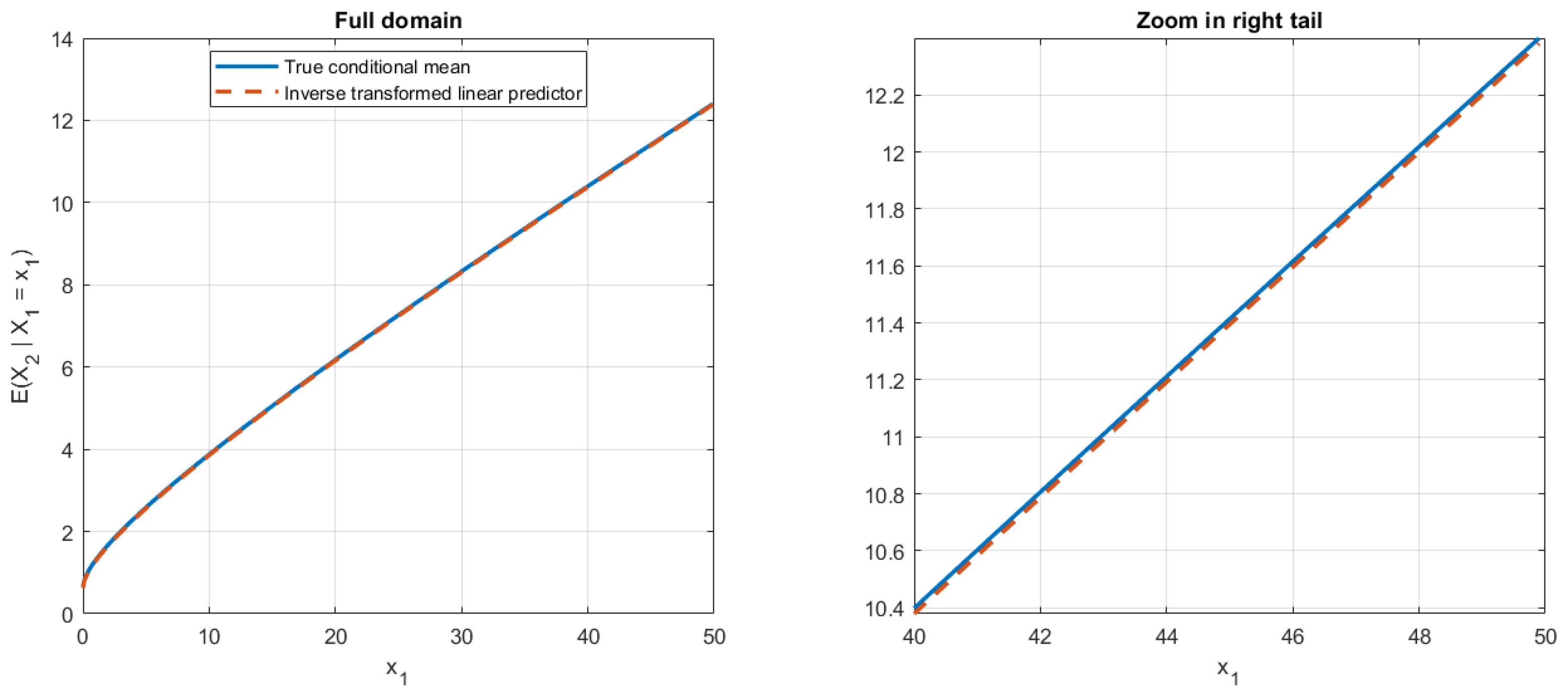
Figure 1 illustrates the same mechanism numerically. The true conditional mean on the original scale is compared with the inverse-transformed linear predictor obtained from the transformed scale. Although the two curves are nearly indistinguishable over most of the domain, the zoom on the right tail reveals a small but systematic discrepancy. This confirms visually that the original-scale conditional mean is not, in general, simply the inverse image of the linear conditional mean in the transformed scale.

Quantitative summary measures for representative parameter configurations are reported in

Table 1. Summary measures of the structural distortion for selected parameter configurations. Here $R_{max}$ denotes the maximum relative distortion over the numerical grid.

${\mathsf{\lambda }}_{\mathit{Y}}$	$\mathsf{\rho }$	${\mathsf{\sigma }}_{\mathit{V}}$	${\mathit{D}}_{max}$	${\mathit{D}}_{\mathbf{rms}}$	${\mathit{R}}_{max}$ (Relative)
0.25	0.50	1.00	$4.47495\times {10}^{-1}$	$3.27621\times {10}^{-1}$	$2.86238\times {10}^{-1}$
0.25	0.80	1.00	$2.65228\times {10}^{-1}$	$1.72324\times {10}^{-1}$	$1.92296\times {10}^{-1}$
0.25	0.95	1.00	$7.95341\times {10}^{-2}$	$4.90362\times {10}^{-2}$	$6.68236\times {10}^{-2}$
0.50	0.80	0.50	$2.26690\times {10}^{-2}$	$2.24999\times {10}^{-2}$	$3.75044\times {10}^{-2}$
0.50	0.80	1.00	$9.07455\times {10}^{-2}$	$8.81265\times {10}^{-2}$	$1.99848\times {10}^{-1}$
0.50	0.80	2.00	$3.62352\times {10}^{-1}$	$3.04694\times {10}^{-1}$	$3.58205\times {10}^{-1}$
0.75	0.80	1.00	$4.43805\times {10}^{-2}$	$3.76786\times {10}^{-2}$	$9.15514\times {10}^{-2}$
1.00	0.80	1.00	$8.88178\times {10}^{-16}$	$2.38561\times {10}^{-16}$	$6.04498\times {10}^{-16}$

. The discrepancy was also evaluated quantitatively over the plotted grid, using the maximum absolute difference, the root-mean-square difference and the maximum relative difference between the two curves. These measures confirm that the discrepancy is numerically small over most of the domain, but systematic and more pronounced in the right-tail region.

The table confirms the analytical predictions and highlights the most extreme configurations. The largest relative discrepancies occur when the conditional dispersion in the transformed scale is larger and the inverse transformation is more strongly nonlinear. For example, increasing ${\sigma }_V$ from $0.5$ to $2.0$, with ${\lambda }_Y=0.5$ and $\rho =0.8$, substantially increases all distortion measures. Conversely, larger values of $\rho$ reduce the distortion by reducing the conditional dispersion of $V\mid U$. The affine case ${\lambda }_Y=1$ provides the benchmark in which the distortion is essentially zero. The scale-free measure $R_{max}$ is particularly useful for comparing parameter configurations, since it expresses the maximum discrepancy relative to the corresponding original-scale conditional mean.

5. Numerical Sensitivity Analysis

The numerical analysis focuses on the range

$$0\le {\lambda }_Y\le 1.$$

This range was chosen in order to include the logarithmic case ${\lambda }_Y=0$, genuinely nonlinear positive transformations, and the affine benchmark ${\lambda }_Y=1$, for which the structural distortion vanishes. The parameters varied in the numerical experiments are

$${\lambda }_Y\in \{0,0.25,0.5,0.75,1\},\rho \in \{0.2,0.5,0.8,0.95\},$$

and

$${\sigma }_V\in \{0.5,1,1.5,2\}.$$

Negative values of ${\lambda }_Y$ are also relevant in applied Box–Cox modelling, but they lead to an upper-bounded admissible domain

$${\mathcal{D}}_{{\lambda }_Y}=(-\infty ,-1/{\lambda }_Y),$$

and may involve stronger interactions between truncation, boundary behaviour and curvature of the inverse transformation. A systematic study of negative transformation parameters is therefore left for future work. Unless otherwise stated, we set ${\lambda }_X=0.3$.

The quantities $M\left(u\right)$, $m_T\left(u\right)$, and ${\tau }_T^2\left(u\right)$ are evaluated by Monte Carlo integration from the conditional truncated normal distribution.

For each parameter configuration and each value of u on the numerical grid, the Monte Carlo integration was performed using $M=2\times {10}^5$ simulated draws from the corresponding conditional normal distribution, retaining only draws in the admissible domain ${\mathcal{D}}_{{\lambda }_Y}$. The same simulation size was used across all parameter configurations. A fixed random-number seed was used to ensure reproducibility. The computations were carried out in MATLAB R2023a using double-precision arithmetic.

The MATLAB script used for the numerical sensitivity analysis and simulated examples is provided as Supplementary Material as Code S1. The second-order approximation to the distortion is given by

$${\Delta }_2\left(u\right)={\displaystyle \frac{1}{2}}{\tau }_T^2\left(u\right)h_{{\lambda }_Y}^{″}\left\{m_T\left(u\right)\right\}.$$

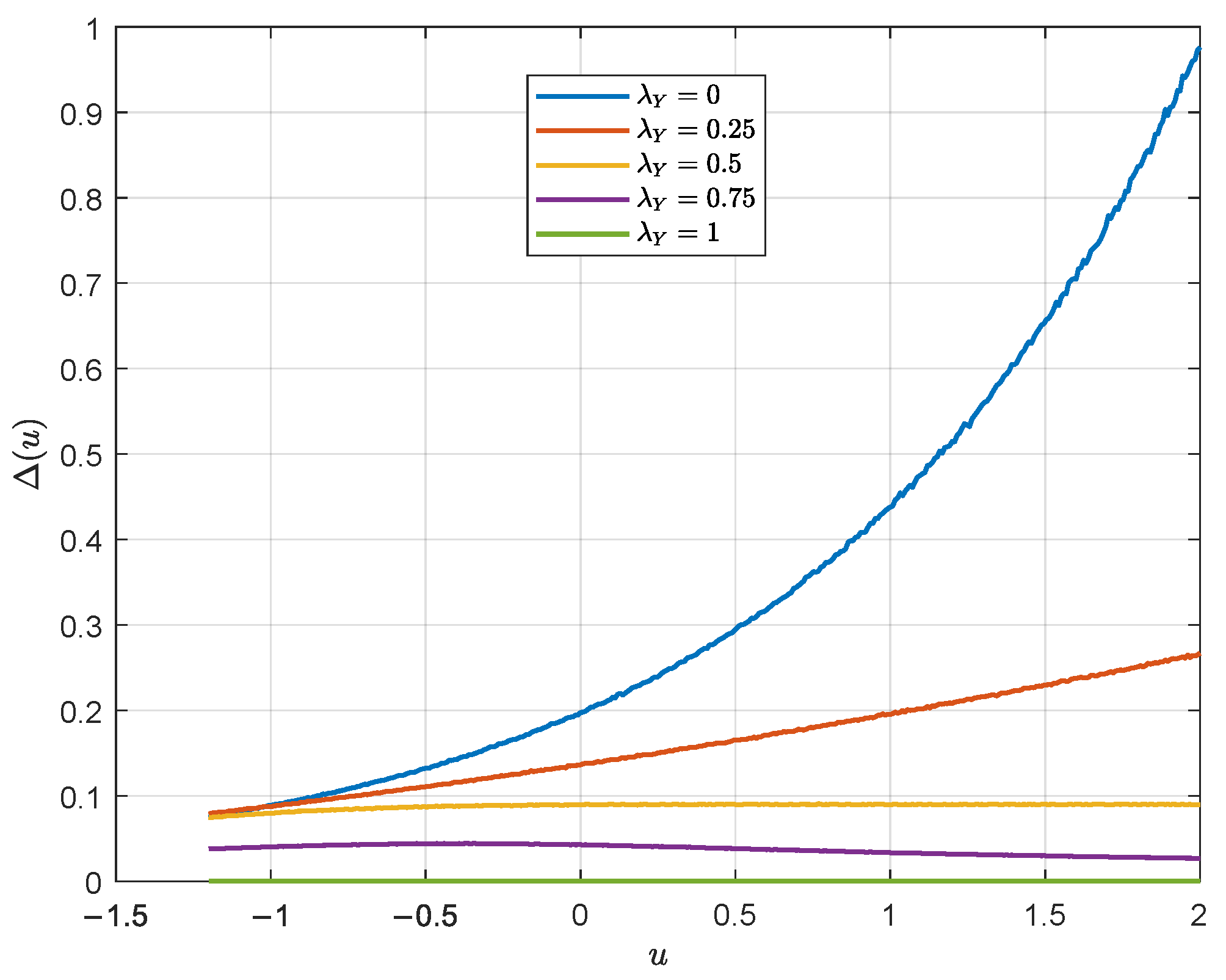
Figure 2 shows the effect of ${\lambda }_Y$, with $\rho =0.8$ and ${\sigma }_V=1$. As expected, the distortion decreases as ${\lambda }_Y$ approaches the affine case ${\lambda }_Y=1$.

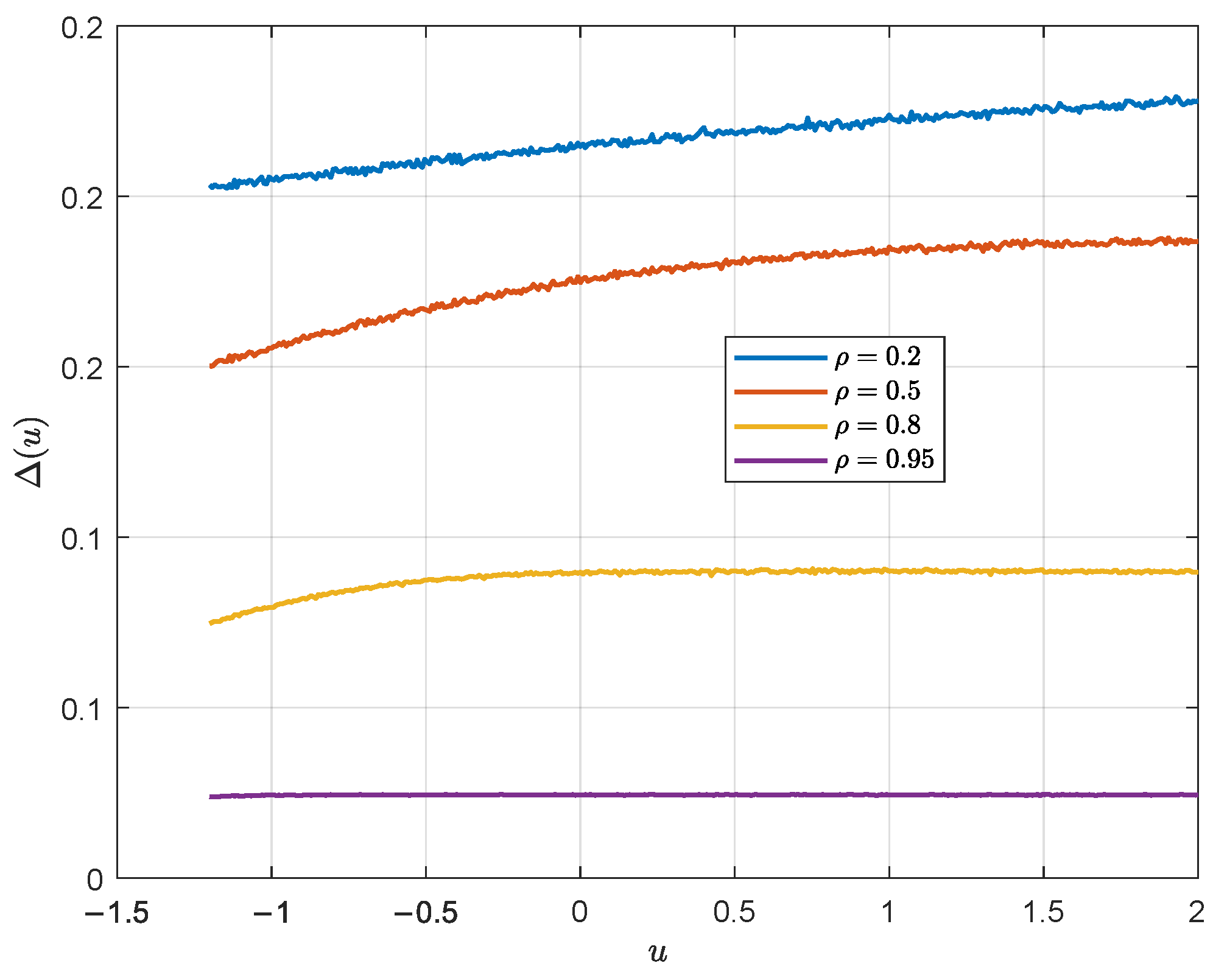
Figure 3 shows the effect of the correlation parameter. Larger values of $\rho$ reduce the conditional dispersion in the transformed scale and therefore attenuate the curvature-induced distortion.

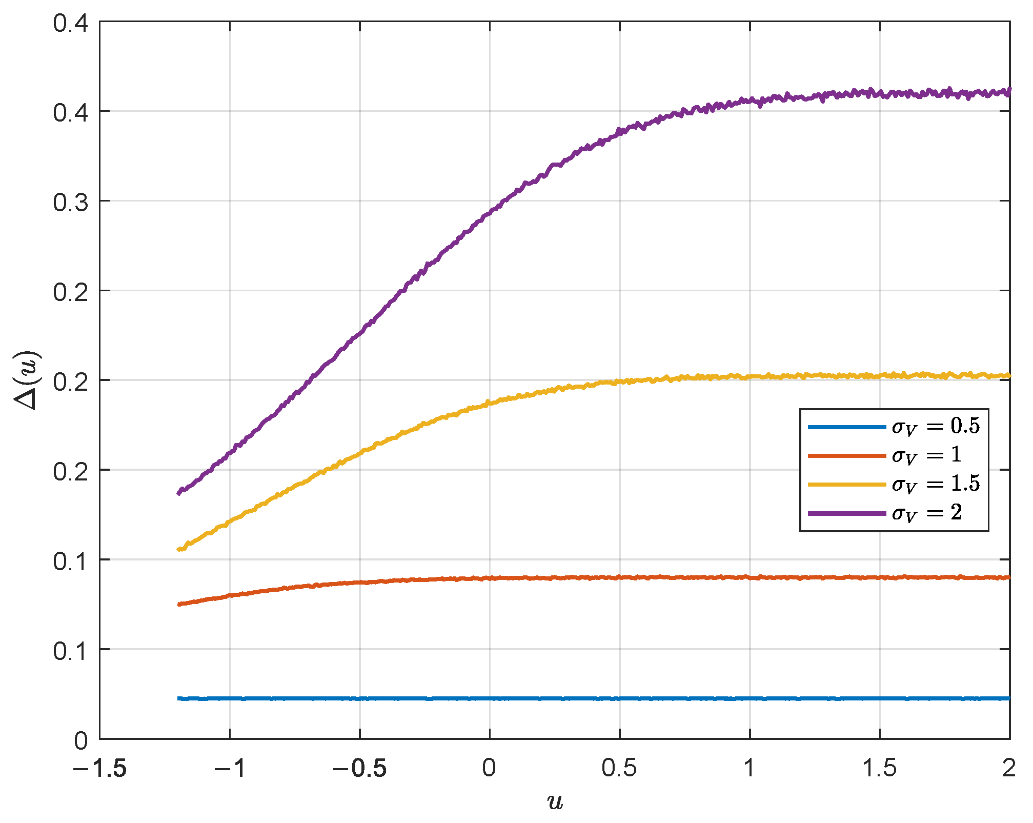
Figure 4 shows the effect of ${\sigma }_V$. Increasing ${\sigma }_V$ increases the conditional dispersion of $V\mid U$, thereby amplifying the distortion induced by the nonlinear inverse transformation.

Here $\mathcal{U}$ denotes the grid of admissible u-values used in the numerical evaluation. To summarize the numerical results, Table 1 reports

$$D_{max}=\underset{u\in \mathcal{U}}{max}|\Delta \left(u\right)|,D_{\mathrm{rms}}={\left\{{\displaystyle \frac{1}{\left|\mathcal{U}\right|}}\sum _{u\in \mathcal{U}}\Delta {\left(u\right)}^2\right\}}^{1/2},$$

and

$$R_{max}=\underset{u\in \mathcal{U}}{max}\left|{\displaystyle \frac{\Delta \left(u\right)}{M\left(u\right)}}\right|.$$

6. A Real-Data Illustration

Let Y denote the variable charges. The MATLAB script used for the real-data insurance illustration is provided as Supplementary Material Code S2. Since Y is strictly positive and strongly right-skewed, it provides a natural empirical setting for a Box–Cox transformation. We fitted a Gaussian linear regression model in the transformed response scale. In the main graphical display, BMI was transformed using ${\lambda }_X=0.5$, and the model included age, transformed BMI, number of children, smoking status, sex, region, and the interactions age × smoker and transformed BMI × smoker as covariates. The response transformation parameter was selected by profile likelihood. The maximum was attained at

$${\widehat{\lambda }}_Y=0.125,$$

indicating a clearly nonlinear transformation of the response variable. For graphical purposes, the fitted curves are displayed as functions of BMI, separately for smokers and non-smokers, with the remaining covariates fixed at reference values. Thus, the figure should be interpreted as a two-dimensional section of the fitted multivariable regression surface, rather than as a simple univariate regression of charges on BMI. For each value of BMI in a grid, and separately for smokers and non-smokers, we computed two fitted curves on the original scale. The first is the usual transform–fit–invert curve,

$${\widehat{m}}_{\mathrm{TFI}}\left(x\right)=g_{{\widehat{\lambda }}_Y}^{-1}\left\{\widehat{E}\left[g_{{\widehat{\lambda }}_Y}\left(Y\right)\mid X=x\right]\right\}.$$

The second is the second-order structural approximation to the conditional mean on the original scale,

$${\widehat{m}}_{\mathrm{SA}}\left(x\right)=g_{{\widehat{\lambda }}_Y}^{-1}\left\{\widehat{\mu }\left(x\right)\right\}+{\displaystyle \frac{1}{2}}{\left(g_{{\widehat{\lambda }}_Y}^{-1}\right)}^{″}\left\{\widehat{\mu }\left(x\right)\right\}{\widehat{\sigma }}^2,$$

where $\widehat{\mu }\left(x\right)$ is the fitted conditional mean in the transformed scale and ${\widehat{\sigma }}^2$ is the residual variance in that scale. For the Box–Cox inverse transformation,

$$g_{\lambda }^{-1}\left(z\right)={(1+\lambda z)}^{1/\lambda },$$

the second derivative is

$${\left(g_{\lambda }^{-1}\right)}^{″}\left(z\right)=(1-\lambda ){(1+\lambda z)}^{1/\lambda -2}.$$

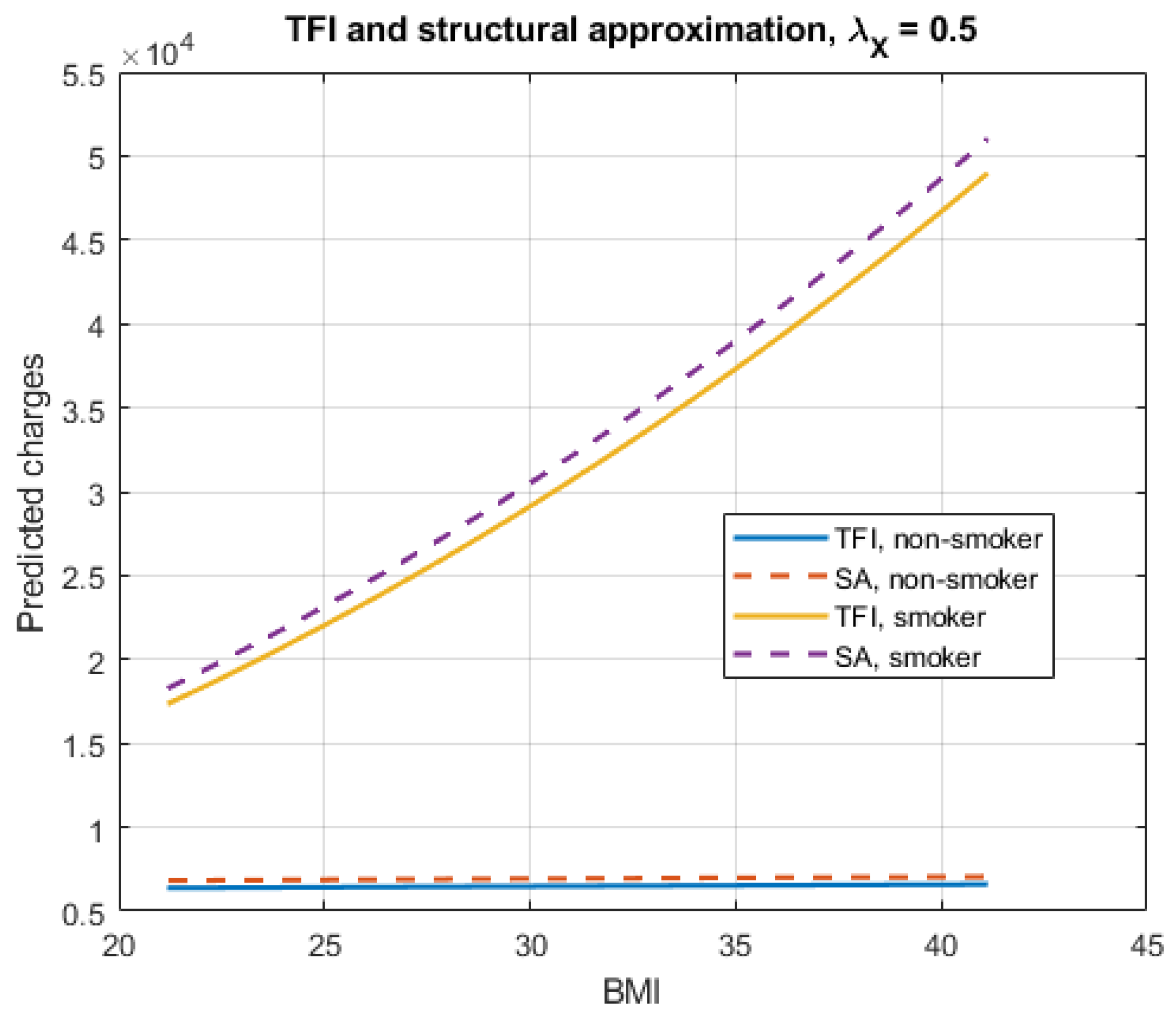
Figure 5 compares the usual transform–fit–invert curves with the corresponding structural second-order approximations. The two curves are close, but they are not identical. The discrepancy is systematic and has the same origin as in the theoretical development: the nonlinear inverse Box–Cox transformation does not commute with conditional expectation.

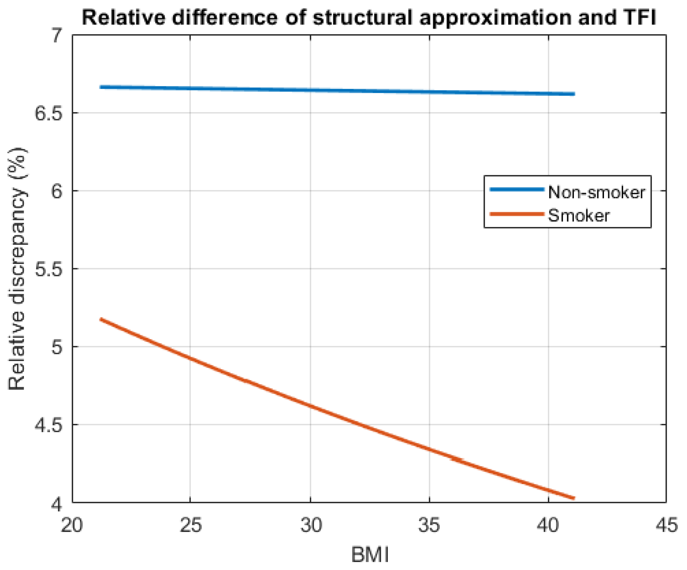
The relative discrepancy

$$100{\displaystyle \frac{{\widehat{m}}_{\mathrm{SA}}\left(x\right)-{\widehat{m}}_{\mathrm{TFI}}\left(x\right)}{{\widehat{m}}_{\mathrm{TFI}}\left(x\right)}}$$

is shown in Figure 6. Over the displayed BMI range, the structural approximation differs from the usual transform–fit–invert predictor by approximately $4\%$ to $7\%$. For non-smokers, the discrepancy is nearly constant, around $6.5\%$, whereas for smokers it ranges from slightly above $5\%$ at lower BMI values to approximately $4\%$ at higher BMI values.

To examine whether the transformation of the explanatory variable affects the magnitude of the discrepancy, we performed a sensitivity analysis with respect to ${\lambda }_X$. The response transformation was kept fixed at the profile-likelihood estimate ${\widehat{\lambda }}_Y=0.125$, while the BMI transformation parameter was varied over the grid

$${\lambda }_X\in \{0,0.125,0.25,0.5,0.75,1\}.$$

For each value of ${\lambda }_X$, the regression model was refitted in the transformed scale, and the relative discrepancy between the transform–fit–invert predictor and the second-order structural approximation was computed over the displayed BMI range and for both smoking groups. The results are reported in

Table 2. Sensitivity of the relative discrepancy to different values of ${\lambda }_X$, with ${\lambda }_Y=0.125$.

${\mathsf{\lambda }}_{\mathit{X}}$	Minimum	Mean	Maximum	Standard Deviation
0	4.1909	5.8075	6.9434	1.1302
0.125	4.1849	5.8087	6.9427	1.1301
0.250	4.1799	5.8107	6.9430	1.1301
0.500	4.1732	5.8175	6.9471	1.1304
0.750	4.1706	5.8280	6.9554	1.1313
1.000	4.1724	5.8419	6.9680	1.1328

.

In this empirical example, the effect of ${\lambda }_X$ on the magnitude of the discrepancy is limited. The mean relative discrepancy varies only from approximately $5.81\%$ to $5.84\%$, while the maximum discrepancy remains close to $7\%$ for all values of ${\lambda }_X$. Thus, although the transformation of the explanatory variable can slightly modify the numerical magnitude of the discrepancy, it does not remove its structural origin. The discrepancy remains a consequence of applying a nonlinear inverse transformation to a conditional summary computed in the transformed response scale. This empirical illustration supports the main message of the paper. Even in a simple real-data regression setting, the curve obtained by fitting a linear Gaussian model in the transformed scale and then applying the inverse Box–Cox transformation should not automatically be interpreted as the conditional mean curve on the original scale. The observed discrepancy is not a numerical artefact of the theoretical examples nor a consequence of a particular choice of ${\lambda }_X$ in this illustration; it is a structural consequence of applying a nonlinear inverse transformation to a conditional summary computed in another scale.

7. Practical Implications and Conclusions

The main practical implication is that an inverse-transformed fitted value should not automatically be interpreted as a conditional mean on the original scale. In the admissible-domain formulation, the inverse-transformed fitted curve is

$$h_{{\lambda }_Y}\left\{m_T\left(u\right)\right\},$$

whereas the conditional mean of the original response is

$$\mathbb{E}[h_{{\lambda }_Y}\left(V\right)\mid U=u,V\in {\mathcal{D}}_{{\lambda }_Y}].$$

These quantities coincide only under special conditions, such as an affine inverse transformation or a degenerate conditional distribution. In general, they answer different statistical questions: the former is the inverse image of a transformed-scale conditional mean, whereas the latter is the mean predictor under squared-error loss on the original scale.

The second-order expansion provides a diagnostic for this discrepancy:

$$C_T\left(u\right)={\displaystyle \frac{1}{2}}{h}_{{\lambda }_Y}^{″}\left\{m_T\left(u\right)\right\}{\tau }_T^2\left(u\right).$$

Thus transformation-based regression should distinguish between the transformed-scale conditional mean, the inverse-transformed fitted curve, and the original-scale conditional mean. Conflating these objects may lead to incorrect interpretation of regression curves, fitted values, conditional effects, and uncertainty summaries on the original scale.

The analysis also clarifies the relation with classical retransformation bias. Retransformation bias is usually concerned with correcting predictions after returning from a transformed scale to the original scale. The perspective developed here is structural: nonlinear inverse transformations do not, in general, preserve the conditional mean operator. This discrepancy is not a finite-sample effect, an estimation error, or a numerical artefact.

Although the paper focuses on conditional means, the same invariance question is relevant for other regression summaries. The answer depends on the statistical functional being considered. Conditional quantiles behave differently from means: under strictly monotone transformations, quantiles are equivariant, so that the inverse transformation of a transformed-scale conditional quantile corresponds to the conditional quantile on the original scale, provided that the conditioning structure is treated consistently. In contrast, conditional variances, prediction intervals and other uncertainty summaries are not generally preserved in a simple way by nonlinear inverse transformations, because such transformations change scale, curvature and dispersion asymmetrically. Thus, the present analysis should be viewed as the conditional-mean case of a broader invariance problem: which statistical summaries are preserved, and which are structurally altered, by transform–fit–inverse modelling procedures. A systematic treatment of quantiles, variances, prediction intervals and other regression summaries lies beyond the scope of the present paper, but represents a natural direction for future work.

The results do not argue against nonlinear transformations. Transformations such as Box–Cox may remain useful for improving normality, stabilizing variance, or simplifying dependence structures. However, once fitted relationships are mapped back to the original scale, the target of interpretation changes unless the non-commutativity with conditional expectation is explicitly accounted for.

From a practical point of view, the structural approximation is most relevant when the target of inference is the conditional mean of the response on the original scale. This includes situations in which inverse-transformed fitted values are used as mean predictions, regression curves are interpreted on the original scale, or covariate effects are discussed after back-transformation. In such cases, the transform–fit–invert curve and the original-scale conditional mean represent different statistical objects.

The magnitude of the discrepancy is expected to be larger when the inverse transformation is strongly nonlinear over the relevant range and when the conditional dispersion in the transformed scale is not negligible. In contrast, if the inverse transformation is nearly affine over the region of interest, or if the transformed-scale conditional variance is very small, the discrepancy may be numerically minor. Practitioners should therefore distinguish between using a transformation as a modelling device in the transformed scale and interpreting inverse-transformed fitted values as mean predictions on the original scale.

Future work may proceed in several directions. One direction is to develop higher-order correction formulas and assess their finite-sample behaviour. Another is to study analogous structural distortions for other transformation families, including transformations designed for zero or negative data. More broadly, the non-commutativity framework may be extended beyond Box–Cox models to other nonlinear transformations, filtering operations, and dependence structures.

Overall, the paper shows that inverse Box–Cox distortion is not merely a technical bias-correction issue. It reflects a structural limitation of nonlinear transformation-based modelling: transformations may simplify the data in one scale, but they do not generally preserve conditional mean structure when mapped back to the original scale.