


Abstract
This article introduces the Evidence Propagation Calculus (EPiC), an operational framework for first-order reasoning built on a simple but productive observation: familiar inference patterns such as Modus Ponens and Modus Tollens behave like the movement of evidential markers across a structured graph. Positive evidence at an antecedent propagates forward to the consequent; negative evidence at a consequent propagates backward. When both markers coexist at a node, the system is locally inconsistent but not operationally broken. To make this observation precise, EPiC grounds reasoning in a four-valued evidential domain , where N denotes absence of evidence, T positive evidence, F negative evidence, and B their coexistence. Each logical connective is assigned a local evidential table, and inference is treated uniformly as the progressive restriction of admissible configurations under an evidential order: inadmissible values are eliminated, minimal surviving values are selected as the next effective evidential states, and the resulting restrictions propagate across shared variables. Compound formulas are decomposed into families of local unary and binary constraints through auxiliary variables, making the propagation process explicit and structurally uniform. Within this setting, Modus Ponens, Modus Tollens, and polarity-switching negation are not postulated as primitive rules. They emerge as derived consequences of the same local table calculus. The framework distinguishes different operational routes of justification. In some cases, positive support reaches the target formula directly through successive local restrictions. In others, propagation first stabilizes the relevant components and the target occurrence is then fixed by the corresponding connective table. Consistency is not a second basic notion of justification but a distinguished property of certain justified outcomes. The article establishes local and global soundness, conservativity over the classical fragment, and a conditional adequacy result. It further develops a translation between decomposed formulas and informational graphs, with a reverse reconstruction theorem for well-formed graphs. The result is a unified operational account of first-order reasoning situated between model-theoretic and proof-theoretic approaches, in which semantics, propagation, and graphical structure are mutually supporting rather than independently layered.
Keywords:
four-valued logic; paraconsistent reasoning; evidence propagation; informational graphs; graph-based reasoning; operational semantics; first-order reasoning; constraint propagation MSC:
03-08
1. Introduction
Reasoning systems are typically presented from one of two familiar perspectives. On the one hand, there is the semantic perspective, which explains logical behavior in terms of valuations, interpretations, and consequence relations. On the other hand, there is the syntactic perspective, which explains reasoning through proof systems, derivation rules, and formal transformations. Both are indispensable. Yet neither, by itself, fully captures an intermediate operational layer in which evidential states evolve under local logical constraints. This layer becomes especially important when reasoning must proceed in the presence of incomplete or conflicting information, where the central issue is not only whether a formula follows from a set of premises, but also how support for that formula is progressively propagated, restricted, stabilized, or excluded across a structured expression.
The present article develops such an operational perspective. It introduces EPiC as a framework for first-order reasoning grounded in a four-valued evidential semantics and a matrix-based propagation calculus. The guiding idea is simple: each connective is associated with a local evidential table, and inference is reconstructed as the progressive restriction of admissible local configurations under an evidential order. At each stage, inadmissible values are removed, minimal surviving values are selected as the next effective evidential states, and the resulting restrictions are propagated across shared variables. In this way, the operational behavior of a formula is not determined by an external stock of connective-specific proof rules, but by a uniform process of local table restriction and reevaluation.
This perspective is particularly natural in the four-valued setting
where N denotes absence of evidence, T positive evidence, F negative evidence, and B the coexistence of both. The resulting semantics is well suited to operational reasoning because it distinguishes not only affirmation and denial, but also informational incompleteness and evidential conflict. This makes it possible to study propagation in settings where inconsistency is not treated as immediate collapse, but as a state that can itself be analyzed operationally. At the same time, EPiC does not allow arbitrary updates. Evidential inconsistency is permitted semantically, whereas operational invalidity is excluded by requiring every update to remain compatible both with the current future-admissible values of the affected variables and with the surviving entries of the local connective tables in which they occur.
EPiC is related to the family of four-valued and paraconsistent semantics associated with Dunn, Belnap, and later developments in the area [1,2], but it is not intended as a mere reformulation of those frameworks. In particular, EPiC shares with Belnap–Dunn style semantics the idea that positive and negative evidence should be treated independently, so that incompleteness and conflict can be represented without collapse. However, its primary aim is different. Rather than focusing mainly on static valuation and consequence over a four-valued domain, EPiC develops an operational account in which evidential values function as local domains of a propagation calculus. In this sense, the framework shifts attention from which evidential states are admissible to how such states evolve, interact, and stabilize across structured formulas. A similar remark applies to evidence-oriented approaches such as Carnielli’s epistemic treatment of evidence and truth [3,4]: EPiC does not compete with them at the level of an alternative philosophical semantics alone, but introduces a local operational mechanism based on connective tables, auxiliary variables, reevaluation, and graph-structured propagation.
A central feature of the framework is that compound formulas are treated through local constraints. Operationally, a complex expression is decomposed into a finite family of unary and binary connective constraints by means of auxiliary variables. This is analogous in spirit to standard auxiliary-variable decompositions used in logic and constraint-based reformulations, including classical transformations of the Tseitin type [5]. What is specific to EPiC, however, is not the mere introduction of auxiliary variables, but their four-valued evidential interpretation together with the invariant linking the admissible values of each variable to the surviving entries of the corresponding connective table. This decomposition makes the propagation process explicit and provides a uniform substrate for the calculus developed in the rest of the article.
Within this setting, familiar inferential patterns such as Modus Ponens, Modus Tollens, and polarity-switching negation are not postulated as primitive rules. They are recovered as derived consequences of the same local table calculus. More generally, the framework distinguishes different operational ways in which a formula may become justified. In some cases, a conclusion is obtained directly through propagation of evidential constraints. In others, propagation stabilizes without explicitly fixing the target formula, and justification is achieved only after a competing denying configuration has been excluded by the relevant connective table or the target compound has been completed through the connective constraint itself. This distinction is operational rather than semantic: it concerns the manner in which support is obtained within the calculus. By contrast, consistency is not treated as a second basic notion of justification, but as a distinguished property of an operationally justified result.
The article also revisits the status of certain patterns that, in more classical presentations, may appear as primitive local rules. In particular, conjunctive and disjunctive inadmissibility are not taken here as independent foundations of the dynamics. Instead, they emerge as derived special cases once the general four-valued propagation mechanism is restricted to the classical fragment. This shift is methodologically significant because it shows that the apparent diversity of local proof-like behaviors can be traced back to a single evidential propagation scheme.
The purpose of the article is therefore twofold. First, it defines the formal basis of EPiC: the four-valued evidential domain, its order structure, the connective operations, the associated local tables, the interpretation structures and satisfaction clauses that underwrite them, and the global propagation mechanism generated by reevaluation of shared variables. Second, it shows, through representative worked examples, how this framework reconstructs familiar first-order reasoning patterns while making explicit both the non-classical roles of the values B and N and the special status of consistency as a property of justified outcomes.
The rest of the article is organized as follows. Section 2 introduces the evidential semantics, interpretation structures, and the matrix-based propagation calculus. Section 3 develops worked examples illustrating direct propagation, paraconsistent propagation, operational silence, quantified connective-level completion, relational reasoning, and cyclic propagation. The subsequent sections connect this operational account with the graphical representation used in EPiC, examine the resulting meta-theoretical properties, and discuss the broader scope and contribution of the framework.
2. Four-Valued Evidential Semantics and Matrix-Based Constraint Propagation
This section develops the formal basis of EPiC. We begin with the interpretation structures and satisfaction relation that underwrite the four-valued semantics, then introduce the evidential order and the connective tables, and conclude with the global propagation mechanism generated by reevaluation of shared variables. Throughout, the key construction is the decomposition of compound formulas into local unary and binary constraints by means of auxiliary variables. Rather than evaluating a complex formula as a whole, EPiC evaluates a network of local constraints relating one output variable to one or two input variables. For example,
is decomposed as
while
is treated as a local implication constraint relating the variables P, Q, and Z. In this way, the value of each auxiliary variable records the evidential value of the corresponding connective occurrence. This decomposition is analogous in spirit to standard auxiliary-variable transformations in logic and constraint-based reformulation, including classical transformations of the Tseitin type [5]. What is distinctive in EPiC, however, is not simply the use of auxiliary variables, but their four-valued evidential interpretation together with the invariant linking the admissible values of each variable to the surviving entries of the corresponding connective table. The decomposition therefore makes the propagation process explicit while preserving a uniform operational structure.
The exposition proceeds from the simplest case to the more structured ones. It begins with implication, since implication is both conceptually basic and structurally present, either directly or indirectly, in the remaining connectives. Its table already displays the central propagation patterns that organize the rest of the section: forward and backward implication propagation under positive evidential value, and polarity-switching behavior under negative evidential value. The same method is then extended to negation, conjunction, and disjunction.
2.1. Interpretation Structures and Satisfaction Relation
Before introducing the matrix-based propagation calculus, we make explicit the semantic interpretation on which it rests. The aim is not to develop a separate model theory in full generality, but to fix the intended reading of the four evidential values and the satisfaction relation underlying the local connective tables.
Definition 1
(EPiC interpretation structure). An EPiC interpretation structure is a pair
where is a first-order domain and ν assigns to each atomic formula an evidential value in
The intended reading is evidential rather than classically truth-functional:
Thus, T means positive evidence only, F negative evidence only, B both, and N no evidence either way. In particular, N is not classical falsity and B is not collapse.
Definition 2
(Assignment and interpretation of terms). Let σ be a variable assignment over D. Terms are interpreted in the standard way. When no confusion arises, we write for the evidential value of a formula φ under and σ.
Definition 3
(Positive and negative satisfaction). A formula φ is positively satisfied in if
and negatively satisfied if
Positive and negative satisfaction are independent; a formula may satisfy either, both, or neither. This is exactly what allows EPiC to represent incompleteness by N and inconsistency by B.
Definition 4
(Semantic clauses). For every interpretation structure and assignment σ, evidential values are defined recursively by:
- 1.
- if φ is atomic, then
- 2.
- 3.
- 4.
- 5.
- 6.
- 7.
- 8.
- 9.
Remark 1.
In clauses (2)–(5), the connectives ¬, ∧, ∨, and → on the right-hand side of each equation denote the four-valued operations defined by the local connective tables introduced in Section 2.5, not the syntactic connectives of the object language appearing on the left-hand side. The recursive definition is therefore not circular: each right-hand-side operation is a function on evidential values, fully determined before the clauses are applied.
These clauses keep affirmation and denial independent: universal positive support requires uniform positive evidence, universal negative support only a counterinstance; existential positive support requires a witness, existential negative support uniform failure.
Definition 5
(Semantic consequence). Let Γ be a set of formulas and φ a formula. We say that Γ semantically supports φ, written , if in every interpretation structure and every assignment σ such that
we also have
The set is the designated set: it collects precisely those evidential values that contain positive evidence, i.e., those with .
Remark 2.
The choice reflects the evidential character of the framework. A formula is semantically supported whenever it carries positive evidence under every consistent assignment to the premises, regardless of whether that evidence is clean (T) or accompanied by conflicting negative evidence (B). The value N is not designated because it represents absence of evidence rather than positive support; the value F is not designated because it carries only negative evidence.
2.2. Evidential Values, Order Structure, and Minimal Future-Admissible Refinement
We now fix the evidential domain on which the whole calculus is based.
Definition 6
(Four-valued evidential domain). Let
where
Here 1 represents positive evidence and 0 negative evidence. Thus, N denotes absence of evidence, T purely positive evidence, F purely negative evidence, and B the coexistence of both.
Definition 7
(Evidential order). Define a binary relation ⪯ on by
Proposition 1.
The structure is a finite partially ordered set. Its strict order is given by
with T and F incomparable.
Proof.
Reflexivity, antisymmetry, and transitivity follow immediately from the corresponding properties of set inclusion. Since
the only strict inclusions are
Moreover, neither nor , so T and F are incomparable. □
Proposition 2.
The ordered set is a finite lattice, with least element N and greatest element B.
Proof.
Since and ⪯ is set inclusion, the meet and join of any two elements of are given by intersection and union, respectively. These operations remain within , so every pair has both a greatest lower bound and a least upper bound. The least element is , and the greatest element is . □
Definition 8
(Future-admissible values). For each , define
Thus, is the upper set generated by x, consisting of the present value x together with all evidential refinements still admissible from it.
Proposition 3.
For the four evidential values, the future-admissible sets are
Proof.
Immediate from the preceding order structure. □
Definition 9
(Minimal surviving values). Let . Define
Proposition 4.
The map may return one or two values. In particular,
Moreover, for every ,
Proof.
The first three equalities follow directly from the order just defined. For the last statement, by reflexivity, and every other element of lies above x. Hence x is the unique minimal element of . □
Remark 3.
EPiC takes the minimum surviving value as the next effective evidential state. This does not eliminate higher surviving values; it only determines the preferred next step in the propagation process.
2.3. A Matrix-Based View of Implication
We now consider the first nontrivial instance of the propagation calculus, namely implication.
Definition 10
(Evidential implication). Define the binary operation
by
Proposition 5.
The operation → is given by the table
Proof.
The entries are obtained by evaluating for all . For example,
The remaining entries are computed analogously. □
Definition 11
(Local implication table). Let P, Q, and Z be variables such that
The local implication table of this constraint is the table above, read as follows: rows correspond to the value of P, columns to the value of Q, and each entry to the value of the output variable Z.
- Initial local state.
Before any restriction takes place, the local state is
Definition 12
(Implication with positive evidential value). The implication constraint is said to have positive evidential value when
Its next effective evidential value is therefore
Proposition 6.
If has positive evidential value, then the local implication table restricts to
with table
Proof.
Starting from the full implication table, one eliminates all entries valued N or F, since only T and B remain admissible at the output variable Z. □
Proposition 7
(Emergent forward implication propagation). Assume that has positive evidential value and that
Then the surviving values of Q are
and its next effective evidential value is T.
Proof.
Restricting P to leaves only the rows T and B. Reading the row corresponding to the current minimum , the surviving values of Q are . Hence
□
Definition 13.
The forward propagation behavior described above will be denoted by
Proposition 8
(Emergent backward implication propagation). Assume that has positive evidential value and that
Then the surviving values of P are
and its next effective evidential value is F.
Proof.
Restricting Q to leaves only the columns F and B. Reading the column corresponding to the current minimum , the surviving values of P are . Hence
□
Definition 14.
The backward propagation behavior described above will be denoted by
Remark 4.
The implication constraint does not always induce a further restriction. For instance, if Z has positive evidential value and , then the consequent remains unrestricted; likewise, if Z has positive evidential value and , then the antecedent remains unrestricted. EPiC therefore distinguishes genuine propagation from operational silence.
Proposition 9.
The patterns and are derived consequences of the local implication table together with minimal-value selection. They are not primitive update rules.
Proof.
Both patterns arise from the same procedure: one first restricts the output variable, then removes inadmissible values, and finally selects the minimum among the surviving values of the relevant input variable. □
2.4. Negation and Polarity-Switching Propagation
We now turn to negation. In the present framework, negation is best understood as the local operation that reverses evidential polarity. Operationally, this polarity reversal can already be observed through the same matrix-based restriction calculus used for implication, once implication is read with negative evidential value.
Definition 15
(Evidential negation). Define the unary operation
by
Proposition 10.
The operation ¬ is given by the table
and satisfies
Proof.
Immediate from the definition. □
Definition 16
(Implication with negative evidential value). The implication constraint is said to have negative evidential value when
Its next effective evidential value is therefore
Proposition 11.
If has negative evidential value, then the local implication table restricts to
with table
Proof.
Starting from the full implication table, one eliminates all entries valued N or T, since only F and B remain admissible at the output variable Z. □
Proposition 12
(Emergent forward polarity switching). Assume that has negative evidential value and that
Then the surviving values of Q are
and its next effective evidential value is F.
Proof.
Restricting P to leaves only the rows T and B. Reading the row corresponding to the current minimum , the surviving values of Q are . Hence
□
Definition 17.
The forward polarity-switching behavior described above will be denoted by
Proposition 13
(Emergent backward polarity switching). Assume that has negative evidential value and that
Then the surviving values of P are
and its next effective evidential value is T.
Proof.
Restricting Q to leaves only the columns F and B. Reading the column corresponding to the current minimum , the surviving values of P are . Hence
□
Definition 18.
The backward polarity-switching behavior described above will be denoted by
Definition 19
(Polarity-switching map). Define the unary map
by
Proposition 14.
For every ,
Proof.
By definition, both maps send
Hence they coincide on all elements of . □
Corollary 1.
Negation is the unary manifestation of polarity-switching propagation.
Proof.
Immediate from the previous proposition. □
2.5. Conjunction and Disjunction as Three-Place Local Constraint Tables
We now extend the matrix-based propagation calculus to conjunction and disjunction. Unlike implication and negation, these connectives do not primarily exhibit directional propagation between two distinguished positions. Instead, they involve a genuinely three-place local interaction among two input variables and one output variable. Their operational behavior is therefore best understood directly through their local evidential tables.
Definition 20
(Evidential conjunction). Define the binary operation
by
Proposition 15.
The operation ∧ is given by the table
Proof.
The entries follow directly from the definition of evidential conjunction. For example,
The remaining entries are obtained in the same way. □
Definition 21
(Local conjunction table). Let P, Q, and Z be variables such that
The local conjunction table of this constraint is the table above, read as follows: rows correspond to the value of P, columns to the value of Q, and each entry to the value of the output variable Z.
Definition 22
(Conjunction with positive evidential value). The conjunction constraint is said to have positive evidential value when
Its next effective evidential value is therefore
Proposition 16.
If has positive evidential value, then the surviving values of both P and Q are
and their next effective evidential values are T.
Proof.
By the conjunction table, only entries valued T or B are compatible with positive evidential value of Z. The surviving rows and columns are therefore T and B only, so both P and Q have surviving values , whose minimum is T. □
Definition 23
(Conjunction with negative evidential value). The conjunction constraint is said to have negative evidential value when
Its next effective evidential value is therefore
Remark 5.
Negative evidential value at a conjunction does not isolate a unique input variable responsible for the negative effective value. Several local configurations may remain admissible.
Definition 24
(Evidential disjunction). Define the binary operation
by
Proposition 17.
The operation ∨ is given by the table
Proof.
The entries follow directly from the definition of evidential disjunction. For example,
The remaining entries are obtained analogously. □
Definition 25
(Local disjunction table). Let P, Q, and Z be variables such that
The local disjunction table of this constraint is the table above, read as follows: rows correspond to the value of P, columns to the value of Q, and each entry to the value of the output variable Z.
Definition 26
(Disjunction with positive evidential value). The disjunction constraint is said to have positive evidential value when
Its next effective evidential value is therefore
Remark 6.
Positive evidential value at a disjunction does not force both input variables toward positive effective values. What it excludes are precisely those local configurations in which neither input is able to support the positive value of the output variable.
Proposition 18.
If has positive evidential value, then neither P nor Q need be individually restricted. However, not every joint assignment of values to P and Q remains admissible.
Proof.
By the disjunction table, the output value T is compatible with several rows and columns when each input is considered separately. However, the entries , , , and do not support positive evidential value of the disjunction. Thus, silence may persist at the level of each input variable taken individually, while failing globally at the level of the pair . □
Definition 27
(Disjunction with negative evidential value). The disjunction constraint is said to have negative evidential value when
Its next effective evidential value is therefore
Proposition 19.
If has negative evidential value, then both P and Q are restricted to
and their next effective evidential values are F.
Proof.
By the disjunction table, the only entries compatible with negative evidential value of the output variable lie in rows F or B and columns F or B. Hence the surviving values of both P and Q are , whose minimum is F. □
Remark 7.
This case is dual to conjunction with positive evidential value. Its detailed table analysis is analogous and is omitted here for brevity.
2.6. Propagation by Reevaluation of Local Constraints
The previous subsections defined the local evidential tables of implication, negation, conjunction, and disjunction. Propagation begins when these local constraints are no longer treated in isolation, but as members of a family linked by shared variables.
For each local constraint, the available evidential values of its output variable must remain consistent with the values still represented by the surviving entries of its associated table, and conversely. Thus, whenever one of the participating variables changes its available or effective evidential values, the corresponding local table must be reevaluated. Operationally, this may be implemented by an interpreter that maintains a pending list of local constraints. As soon as the value of an output variable or of one of its input variables is modified, every local constraint containing that variable is placed on the pending list and recomputed. The only essential requirement on this reevaluation mechanism is that one local table be updated at a time. This suffices to prevent a value already eliminated from the current future-admissible domain of a variable from being reintroduced by a later step.
Definition 28
(Global evidential state). A global evidential state is the family of current available evidential value sets assigned to all variables together with the currently restricted local tables associated with all connective constraints.
Definition 29
(Stabilized global state). A global evidential state is stabilized if reevaluation of all pending local constraints yields no further restriction of any available evidential value set.
Definition 30
(Operational validity). An operational evolution is valid if every update assigned to a variable belongs to its current set of future-admissible values and remains compatible with the surviving entries of every local table in which that variable occurs.
Remark 8.
EPiC allows evidential inconsistency, represented by the value B, but it does not allow operational invalidity. Once a value has been eliminated from the future-admissible domain of a variable, no legitimate propagation step may reintroduce it.
Proposition 20
(Monotonicity of propagation). During propagation, the set of available values of each variable can only stay the same or shrink.
Proof.
Each reevaluation step deletes values that are no longer compatible with the currently restricted local tables. It never reintroduces values that have already been eliminated. □
Proposition 21
(Finite termination). If the formula under consideration gives rise to only finitely many connective constraints, then every propagation process terminates after finitely many reevaluation steps.
Proof.
Each variable has a finite set of available values, namely a subset of . By monotonicity, reevaluation can only shrink these sets. Since there are finitely many variables and finitely many possible value sets, only finitely many strict reductions can occur. □
Remark 9.
The purpose of the propagation mechanism is not to add a second layer of independent rules on top of the local tables. Its role is simply to ensure that every local restriction is transmitted to all other constraints sharing the affected variables. In this way, the local matrix calculus becomes a propagation calculus for structured formulas.
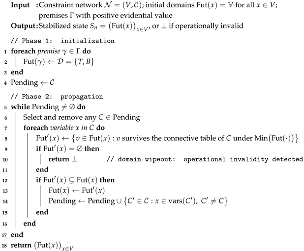
The propagation process described above admits a precise algorithmic formulation. Algorithm 1 specifies it in terms of a pending list of constraints to be reevaluated, making the termination guarantee and the detection of operational invalidity explicit.
| Algorithm 1: EPiC propagation over a constraint network |
 |
Remark 10
(Correctness and complexity of Algorithm 1). Termination follows from the monotonicity of propagation (Proposition 20): each iteration either strictly reduces some or leaves all domains unchanged, and domains have minimum size one. Since and there are n variables, at most domain reductions can occur. Each reduction re-enqueues at most the adjacent constraints; since each incidence is triggered at most 3 times, the total number of reevaluation steps is where m is the number of variable-constraint incidences. The ⊥ return on wipeout implements the detection of operational invalidity: once a domain is empty, no future-admissible value exists for that variable, which violates Definition 30.
2.7. Derived Classical Patterns and the Status of Conjunctive and Disjunctive Inadmissibility
The matrix-based propagation calculus developed in the previous subsections changes the status of conjunctive and disjunctive inadmissibility. In the present framework, these patterns are no longer required as primitive operational rules. The global behavior of the calculus is already determined by local evidential tables, restriction of admissible values, minimal-value selection, and reevaluation of shared variables. What remains is to explain how the familiar classical patterns reappear as derived consequences.
Definition 31
(Classical fragment). The classical fragment of the evidential domain is the subdomain
Proposition 22.
The restrictions of the conjunction and disjunction tables to are
respectively.
Proof.
Delete the rows and columns labeled N and B from the full conjunction and disjunction tables. The remaining entries are exactly those displayed above. □
Definition 32
(Classical conjunctive admissibility and CI). Let be restricted to the classical fragment
and let . The corresponding admissible conjunctive triples are
A triple is classically conjunctively admissible if
It is classically conjunctively inadmissible, or a case of classical conjunctive incompatibility , if
Equivalently,
Proposition 23
(CI as complement of the restricted conjunction table). Classical conjunctive incompatibility is exactly the complement of the restricted conjunction table in . In particular,
Hence:
- 1.
- The triple is incompatible;
- 2.
- If is admissible for , then and ;
- 3.
- If is admissible for , then at least one of must be F;
- 4.
- If , then the only admissible value of z is T.
Proof.
The restricted conjunction table determines exactly the ternary relation
Since contains all possible classical triples , every triple not belonging to is inadmissible. Therefore
The listed consequences follow immediately by inspection of . □
Definition 33
(Classical disjunctive admissibility and DI). Let be restricted to the classical fragment
and let . The corresponding admissible disjunctive triples are
A triple is classically disjunctively admissible if
It is classically disjunctively inadmissible, or a case of classical disjunctive incompatibility , if
Equivalently,
Proposition 24
(DI as complement of the restricted disjunction table). Classical disjunctive incompatibility is exactly the complement of the restricted disjunction table in . In particular,
Hence:
- 1.
- The triples , , and are incompatible;
- 2.
- The triple is also incompatible;
- 3.
- If is admissible for , then and ;
- 4.
- If at least one of is T, then the only admissible value of z is T.
Proof.
The restricted disjunction table determines exactly the ternary relation
Since contains all possible classical triples , every triple not belonging to is inadmissible. Therefore
The listed consequences follow immediately by inspection of . □
Proposition 25
(Derived status of CI and DI). CI and DI are derivable from the matrix-based propagation calculus on the classical fragment.
Proof.
On the classical fragment, conjunction and disjunction are represented by the restricted ternary relations
Propagation eliminates precisely those local triples that do not belong to the corresponding relation. Therefore CI and DI are not primitive rules. They are names for the inadmissibility of local triples excluded by the restricted conjunction and disjunction tables. □
Corollary 2.
The classical local patterns of conjunction and disjunction are special cases of the general matrix-based propagation calculus obtained by restricting the evidential domain to
Proof.
Immediate from Propositions 23–25. □
The contribution of this section is both formal and methodological. Formally, it fixes the four-valued evidential domain, the associated order structure, the connective operations and their local tables, the restriction calculus based on minimal effective values, and the propagation mechanism based on reevaluation of shared variables. Methodologically, it shows that EPiC is not organized around an expanding list of primitive connective-specific rules. Instead, a single matrix-based propagation scheme gives rise to the familiar operational behaviors of implication, negation, conjunction, and disjunction. In the classical fragment, CI and DI reappear as names for the inadmissibility of local triples excluded by the restricted conjunction and disjunction tables, but they no longer function as the foundation of the dynamics itself.
3. Operational Justification: Worked Examples
The formal machinery introduced in the previous section becomes easier to appreciate when examined in concrete cases. We therefore revisit several representative first-order reasoning patterns and analyze them in EPiC terms. The point of these examples is not merely illustrative. They show how the abstract propagation calculus operates on structured formulas and how operational justification can arise through different configurations of propagation, local completion, inconsistency, silence, relational structure, and cyclic dependency.
The first example exhibits the simplest stabilization pattern: a conclusion acquires positive evidence directly through the propagation of an informational implication. The subsequent examples make explicit the specifically non-classical behavior of the framework by showing how EPiC handles evidential inconsistency, absence of propagated support, relational structure, and cycles in the underlying informational network.
3.1. Reasoning by Propagation: The Socratic Example
We begin with an elementary example whose role is to display the simplest propagation pattern of the calculus.
Let the language contain unary predicates H (“is human”) and M (“is mortal”), together with a constant symbol s denoting Socrates. Consider the premises
and the intended conclusion
In EPiC, premise (1) is not treated as a primitive proof rule. Rather, once the individual s is fixed, it induces the informational implication
Equivalently, at the level of local constraints, one may introduce an auxiliary variable Z and write
with Z carrying positive evidential value by virtue of premise (1). The local behavior is then governed by the implication table analyzed in Section 2.3.
Justification by Propagation
Assume that premise (2) contributes positive evidence:
Since the informational implication associated with
requires
the value of must be restricted so as to preserve that inclusion. In the terminology of Section 2.3, once carries current effective positive evidence, the corresponding implication pattern propagates positive evidence forward to . Hence one obtains
No connective-specific exclusion is needed at this stage. The conclusion receives positive evidence directly through the propagation of the informational constraint. This is the basic pattern of justification by propagation.
Proposition 26.
In the Socratic syllogism, is operationally justified by propagation. Moreover, on classically consistent inputs, this justification is consistent.
Proof.
Premise (2) gives
Premise (1) induces the informational implication
The corresponding local restriction propagates positive evidence to
so
Thus is operationally justified by propagation. If the initial configuration is classically consistent, then, by conservativity, the operational fixpoint remains two-valued, so
and the resulting justification is consistent. □
The same example also admits a complementary instability reading. Suppose, for the sake of analysis, that one tentatively imposes
Then the informational implication
forces the corresponding backward propagation of negative evidence to
Since
already holds, the occurrence becomes evidentially inconsistent. This does not invalidate the configuration, since inconsistency is permitted in EPiC. What it shows is that denying the conclusion produces immediate tension with the informational structure induced by the premises.
Figure 1 records both operational readings. Panels (a)–(d) trace the forward propagation of positive evidence from to ; panels (e)–(h) trace the backward propagation of negative evidence in the instability reading, producing an evidentially inconsistent state at .
Figure 1.
Operational analysis of the Socratic syllogism in EPiC. Panels (a–d) illustrate justification by propagation: positive evidence for induces, through the informational implication , positive evidence for . Panels (e–h) illustrate the complementary instability reading: assuming negative evidence for propagates negative evidence backward to , yielding an evidentially inconsistent assignment at . The figure records an evolution of evidential assignments under informational constraints, not a proof-theoretic derivation. Node fill color indicates evidential status: green denotes a node currently carrying positive evidence, red denotes negative evidence, and an unfilled (white) node denotes a formula occurrence with no evidence yet established; arrows denote UI-edges of informational implication.
3.2. A Paraconsistent Example with the Value B
To make the non-classical behavior of the framework explicit, consider the following paraconsistent configuration. Let A, B, C, D, and E be unary predicates, and assume:
From (1), a witness a satisfies
so
By , positive evidence for yields
and therefore
Forward propagation through (2) and (4) yields
while backward propagation through (3) and (5) yields
Thus a local inconsistency at produces structured consequences without explosion.
Proposition 27.
In the configuration determined by premises (1)–(5), the witness a induces an evidentially inconsistent occurrence with value B, while supporting the non-trivial consequences
Proof.
The witness a is obtained from (1). Conjunction elimination gives positive evidence for both and , and therefore yields negative evidence for . Hence . Forward propagation through (2) and (4) yields positive evidence for and . Backward propagation through (3) and (5), using the negative evidence already available at and , yields negative evidence for and . □
3.3. A Worked Example with Quantifiers and Conjunction
We now consider a more structured example whose purpose is to show how EPiC handles the joint action of quantifiers, implication, and conjunction within a single operational configuration. Unlike the Socratic case, where one informational implication is enough to support the conclusion directly, the present example exhibits a more articulated process. Propagation first determines the relevant component occurrences, and the local table of the target conjunction then determines how the compound conclusion is completed.
- Statement of the argument.
Let A, B, and C be unary predicates. Assume the premises
and the intended conclusion
From premise (2), existential instantiation introduces a witness a such that
By the semantic clause for conjunction, this yields
By the semantic clause for negation, we therefore obtain
Premise (1) induces, for the instance a, the informational implication
Equivalently, this may be represented by a local implication constraint
with Z carrying positive evidential value. Since
the corresponding backward implication pattern propagates negative evidence to
Thus
and, by negation once more,
At this stage the system has established
Introduce an auxiliary variable Y for the target conjunction:
Once both component occurrences carry positive evidential support, the local conjunction table restricts the admissible values of Y. In particular, the local configuration in which both conjuncts carry positive evidence while the conjunction remains negatively fixed is not admissible in the classical fragment of the conjunction table. The connective table therefore eliminates that alternative and leaves the positively supported conjunctive value as the admissible continuation.
Accordingly, one obtains
that is,
By existential introduction,
Proposition 28.
The conclusion is operationally justified from premises (1) and (2) through witness instantiation, backward implication propagation, and local completion by the conjunction constraint.
Proof.
Premise (2) yields
hence
Premise (1) induces the informational implication
so the corresponding backward propagation yields
and therefore
Let
Since both conjuncts now carry positive support, the local conjunction table eliminates the incompatible alternative in which the conjunction would fail to receive positive support. Hence
that is,
Existential introduction then yields
□
Figure 2 records the operational structure of this example. Panel (a) provides a natural-deduction rendering of the derivation as a structural guide; panel (b) shows the corresponding informational graph. Labels of the form indicate the correspondence between a graph node, the step (3) in panel (a), and the evidential value assigned to that node at stabilization.
Figure 2.
Operational analysis of the quantified conjunction example in EPiC. Panel (a) presents a natural-deduction rendering of the formulas involved and is included only as a structural guide. Panel (b) shows the corresponding informational graph. Labels of the form indicate the correspondence between a graph node, the step in panel (a), and the evidential value assigned to that node. UI-arrows encode evidential inclusion as local informational constraints. Node fill color follows the same convention as Figure 1: green indicates positive evidence () and red indicates negative evidence (), with corresponding green UI-edges and red UC-links between nodes. The example illustrates the coordinated action of witness instantiation, backward implication propagation, and conjunctive completion within a single operational configuration.
The informational graph in panel (b) of Figure 2 makes the operational structure explicit: witness instantiation and backward propagation fix the component occurrences, and the target conjunction is then completed by the local connective constraint. This pattern—propagation determining the components, the connective table completing the compound—is the characteristic operational signature of conjunctive completion in EPiC.
3.4. Operational Silence and the Value N
The value N becomes visible when a local configuration supports neither propagation nor denial. Consider the implication constraint
with
Under positive evidential value of the implication, the restricted implication table shows that when the current minimum of P is F, all four values remain admissible for Q:
Hence the implication imposes no restriction on the consequent. If no other constraint affects Q, then its next effective evidential value is
Proposition 29.
Let be a local implication constraint with
Then the consequent remains unrestricted,
and if no other constraint affects Q, its next effective evidential value is N.
Proof.
Under positive evidential value of the implication, only entries valued T or B survive. Restricting the antecedent to and reading the row for the current minimum , all four values remain admissible for the consequent. Hence no restriction is imposed on Q, and its next effective value remains N when no other constraint intervenes. □
3.5. A Relational Example
To make the expressive scope of the framework explicit, consider a simple example involving a binary predicate. Let and be unary predicates, and let mean that y is the head of x. Assume:
The intended conclusion is
From (2) and the implication induced by (1), forward propagation yields
Premise (3) gives
Introducing
conjunction yields
that is,
By existential introduction with witness a, one obtains
Proposition 30.
From premises (1)–(3), EPiC operationally justifies
Proof.
Premise (2) gives positive evidence for . Premise (1) induces , so yields positive evidence for . Together with premise (3), the conjunction constraint yields positive evidence for , and existential introduction then yields the conclusion. □
Remark 11
(Uniform generalisation and the De Morgan pattern). The specific choices of individual a and head h in this example are inessential. The same reasoning pattern applies to any individual b and any head k: from and , the same sequence of forward implication propagation, conjunction, and existential introduction yields . Since no property particular to a or h was exploited, the argument generalises uniformly.
In EPiC, universal conclusions of the form
are recovered by noting that the instance-level operational reasoning succeeds for every instantiation of x and y. The universal constraint is therefore operationally satisfied across all relevant instances. This is the De Morgan inference pattern in the relational case: a structural property of individuals transfers systematically to a structural property of their parts, and EPiC reconstructs the transfer through local propagation rather than through a dedicated structural inference rule.
3.6. A Cyclic Network Example
We now consider a slightly larger network containing both a local inconsistency and a cycle. Let P, Q, and R be unary predicates, and assume:
Thus the informational dependencies form the cycle
From (1), existential instantiation introduces a witness a such that
Hence
so
Forward propagation through (2) and (3) yields positive evidence for and . Since and negative evidence already holds at , backward propagation through (4) yields negative evidence for , which then propagates backward through (3) to . Hence
The cycle therefore produces a stabilized inconsistent state without explosion: no arbitrary formula outside the cycle is forced, and reevaluation terminates because admissible-value restriction is monotone over a finite domain.
Proposition 31.
In the cyclic configuration determined by premises (1)–(4), the witness a induces evidentially inconsistent occurrences at , , and , each of value B, and the resulting propagation stabilizes without trivialization.
Proof.
The witness a is obtained from (1). As before, yields negative evidence for , so . Forward propagation through (2) and (3) yields positive evidence for and . Since negative evidence already holds at , backward propagation through (4) and then through (3) yields negative evidence for and . Thus all three occurrences take value B, and stabilization follows from finiteness and monotonicity. □
Taken together, these examples show that EPiC handles direct propagation, connective-mediated completion, explicit paraconsistency, operational silence, relational structure, and cyclic dependency within a single evidential framework.
4. Informational Graphs and Graph Translation
The informational graphs of EPiC did not arise as an afterthought. The original motivation for the framework was visual: Modus Ponens and Modus Tollens as movements of evidential markers across a structured diagram, with nodes representing propositions and edges representing the direction of propagation. The matrix-based calculus of Section 2 is the formalization of that picture. This section makes the correspondence explicit by defining the graphical vocabulary, the translation from formulas to graphs, and—crucially—the reverse reconstruction that shows the translation is not a lossy encoding but a genuine structural equivalence.
The graphs introduced here are not diagrams added for exposition. They are a structural presentation of the same propagation network already defined through the local tables. A node is an evidential variable. An edge is a local dependency. The graph makes visible the constraint architecture that the table calculus leaves implicit.
4.1. Graphical Vocabulary
Two kinds of edges are needed, and only two. They correspond exactly to the two propagation behaviors identified in Section 2: evidential inclusion () and polarity switching ().
Definition 34
(Informational graph). An informational graph is a finite directed graph
where:
- V is a finite set of nodes;
- is the set of UI-edges;
- is the set of UC-edges.
Each node is typed by an evidential variable and carries an available evidential value set over .
The evidential domain carries the same reading as before:
Definition 35
(Primitive graph constraints). Let assign to each node its current set of available evidential values. Then:
- 1.
- For each UI-edge , the edge records an evidential inclusion constraint from u to v;
- 2.
- For each UC-edge , the edge records a polarity-switching dependency between u and v.
At the level of effective values, these correspond to the propagation behaviors and .
Remark 12.
A UI-edge expresses evidential inclusion; a UC-edge expresses polarity switching between opposite-polarity occurrences of the same informational item. The graph vocabulary introduces no new logical primitives. It makes explicit the two local dependency patterns already isolated in the propagation calculus.
Definition 36
(Well-formed UC-edge). A UC-edge is well formed only if u and v represent opposite-polarity occurrences of the same informational item.
Proposition 32.
For every evidential value ,
Hence a UC-edge may be read in either direction without introducing a second polarity-switching primitive.
Proof.
Immediate from the definition of in Section 2.4. □
Remark 13.
The orientation of UI-edges is operational, not merely graphical. It determines the direction of evidential propagation: forward propagation corresponds to and backward propagation to , as defined in Section 2.3. Reversing a UI-edge would reverse the direction of constraint flow, not merely the visual appearance of the diagram.
4.2. Constraint Decomposition and Graph Construction
The graph of a formula is obtained in two conceptually distinct steps. First, one reads the formula recursively as a syntactic tree: the root is the main connective of the formula, and the children of that root are the roots of the trees associated with its immediate subformulas. Atomic formulas are leaves. Second, this syntactic tree is operationalized by introducing evidential variables for formula occurrences and by replacing connective occurrences with local unary or binary constraints.
This distinction is important. The graphical representation is not an arbitrary diagram attached to a formula after the fact. It is a homomorphic image of the recursive syntactic structure of the formula, enriched with the operational dependency information required by the EPiC calculus.
Definition 37
(Recursive formula tree). Let φ be a first-order formula. The recursive formula tree is defined as follows:
- 1.
- If φ is atomic, then consists of a single node labelled by φ;
- 2.
- If , then the root of is labelled by ¬, and its unique child is the root of ;
- 3.
- If , with , then the root of is labelled by ∘, and its two children are the roots of and ;
- 4.
- If , with , then the root of is labelled by , and its unique child is the root of .
Definition 38
(Occurrence-variable assignment). Let φ be a formula and let be the set of syntactic occurrences of subformulas of φ. An occurrence-variable assignment maps each occurrence to an evidential variable . If ψ is atomic, then may be identified with the atomic occurrence itself. If ψ is compound and is not the root occurrence of φ, then is a fresh auxiliary variable. If the whole formula is written as , then the root variable is .
Definition 39
(Constraint decomposition). Let φ be a formula equipped with an occurrence-variable assignment. The constraint decomposition of φ, denoted , is obtained recursively from as follows:
- 1.
- If ψ is atomic, then no connective constraint is introduced;
- 2.
- If , then introduce the unary local constraint
- 3.
- If , then introduce the binary local constraint
- 4.
- If , then introduce the binary local constraint
- 5.
- If , then introduce the binary local constraint
- 6.
- If , then the biconditional is treated as a definitional abbreviationThus, introduce fresh variables and and add the constraintsHence no new primitive graph edge is required for ↔.
- 7.
- if , with , then the quantifier contributes the instance- or witness-level variables required by the operational context, together with the local constraints generated by the corresponding instantiated body .
Example 1.
For
the root variable is . The non-root compound occurrence receives a fresh auxiliary variable X, and the decomposition is
Thus the decomposition follows the recursive syntax tree, but replaces the internal connective occurrence by the auxiliary variable X.
Example 2.
For
the inner implication receives a fresh auxiliary variable X. The decomposition is
Thus the operational graph remembers the right-nested syntactic structure of the formula.
Example 3.
For
the internal conjunction receives a fresh auxiliary variable X, and the decomposition is
The corresponding graph contains the conjunctive UI-pattern for and a UC-link between X and Z.
Definition 40
(Graph translation). Let φ be a formula with constraint decomposition . The informational graph is the decorated graph obtained as follows:
- 1.
- Every occurrence variable appearing in becomes a node.
- 2.
- Every unary negation constraintcontributes a UC-link between the nodes and . Since UC is involutive, this link may be drawn as a bidirectional red edge, or equivalently as two opposite UC-arcs:
- 3.
- Every implication constraintcontributes a directed UI-edge from the antecedent node to the consequent node:The output variable is not erased. It is retained as the variable associated with that implication occurrence, either as an explicit edge label or as a small node placed on the corresponding edge. This is necessary for reverse reconstruction.
- 4.
- Every disjunction constraintcontributes two directed UI-edges toward the disjunction node:Thus the disjunction occurrence is the common destination of its component occurrences.
- 5.
- Every conjunction constraintcontributes two directed UI-edges away from the conjunction node:Thus the conjunction occurrence is the common source of its component occurrences.
- 6.
- Every biconditional occurrence is translated through its definitional decomposition:Consequently, its graph consists of the two implication UI-edgestogether with the conjunction pattern linking to and .
- 7.
- Quantified formulas contribute only the instance- or witness-level variables introduced in the operational context. The local graph structure of each instantiated body is then generated by the preceding clauses. No additional primitive edge type is needed for quantifiers.
Remark 14.
The colors used in visual drawings may indicate the current evidential value of the corresponding occurrence or constraint. For example, a positive implication occurrence may be drawn with a green UI-edge, while a negative implication occurrence may be drawn with a red indication of the corresponding denying configuration. These colors are visual annotations of evidential state. The underlying syntactic translation is determined by the recursive structure of the formula and by the local constraint associated with each connective occurrence.
Remark 15.
The output variable of an implication occurrence must remain available in the decorated graph, even when it is drawn as an edge label. Otherwise, the graph would remember that there is a dependency from antecedent to consequent, but would lose the occurrence variable corresponding to the formula . This would make reverse reconstruction ambiguous.
Proposition 33
(Finiteness and structural faithfulness of graph translation). For every first-order formula φ, the graph translation is finite up to the set of grounded instances or witnesses explicitly introduced in the reasoning context. Moreover, is structurally faithful to the recursive formula tree , up to the introduction and renaming of auxiliary occurrence variables.
Proof.
The formula tree is finite because is a finite syntactic object. The occurrence-variable assignment introduces one variable for each relevant formula occurrence and, in the case of definitional expansions such as the biconditional, only finitely many additional auxiliary variables. Each connective occurrence contributes exactly one local constraint, except for abbreviations such as ↔, which are first expanded into finitely many primitive constraints. Quantifiers contribute only the instance- or witness-level variables actually introduced in the operational context. Hence the resulting graph is finite relative to that context.
Structural faithfulness follows by induction on the recursive construction of . Atomic occurrences become nodes. Negation occurrences become UC-links between the negated occurrence and its subformula. Binary connective occurrences become directed UI-patterns determined by their connective type: implication from antecedent to consequent, disjunction from components to output, and conjunction from output to components. Therefore the graph preserves the immediate subformula structure of the syntax tree, enriched with the operational orientation required by the EPiC propagation calculus. □
4.3. Well-Formed Informational Graphs
Not every labeled directed graph with two edge types is a meaningful EPiC structure. Well-formedness is the condition that a graph still remembers the decomposition from which it came—a requirement that makes reverse translation possible.
Definition 41
(Well-formed informational graph). An informational graph is well formed if:
- 1.
- Every node is typed by a unique evidential variable;
- 2.
- Every UC-edge satisfies Definition 36;
- 3.
- Every UI-edge has a direction compatible with the connective constraint from which it arises:
- If the graph encodes an implication constraint , then the corresponding UI-edge is directed from P to Q;
- If the graph encodes a disjunction constraint , then the corresponding UI-edges are directed from the component variables toward the disjunction node:
- If the graph encodes a conjunction constraint , then the corresponding UI-edges are directed from the conjunction node toward the component variables:
- 4.
- Every output variable of a unary or binary constraint is linked to the variables of its immediate input subexpressions in a way compatible with the corresponding connective table;
- 5.
- Every quantified variable is associated with the instance- or witness-level variables introduced by the operational context;
- 6.
- The graph arises from a finite constraint decomposition of a first-order formula.
Remark 16.
Well formedness is not a matter of graphical neatness. It is a structural condition: a well-formed graph retains exactly the information needed to reconstruct the formula from which it came. Directional correctness of UI-edges is not optional—evidential propagation depends on it, and without it the reverse translation fails.
Proposition 34
(Subformula closure). If , then the node labels of G are closed under the decomposition of φ into immediate connective subexpressions, up to the instance and witness expansions introduced by quantifiers.
Proof.
Immediate from the recursive construction of the constraint decomposition. □
4.4. From Informational Graphs Back to Formulas
The translation just defined is not merely one-way. Under the well-formedness conditions above, a formula can be reconstructed from its informational graph. The purpose of the present result is to show that the graphical layer is structurally faithful to the decomposition scheme introduced in Section 4.2.
Theorem 1
(Reverse reconstruction). For every well-formed informational graph generated by the translation scheme, there exists a first-order formula whose constraint decomposition yields that graph, up to graph isomorphism and renaming of bound variables or witnesses.
Proof.
Let G be a well-formed informational graph generated by the translation scheme. We show that G can be folded back into a first-order formula by induction on the number of output variables introduced by the decomposition.
- Base case. If the graph contains no output variable introduced by a unary or binary connective constraint, then every node corresponds to an atomic occurrence. In that case, reconstruction is immediate: each node yields an atomic formula, and the graph corresponds to a finite atomic fragment, up to renaming of variables or witnesses.
- Unary case. Suppose u and v are connected by a UC-edge. Since the graph is well formed, Definition 36 guarantees that these two nodes represent opposite-polarity occurrences of the same informational item. Hence one of them reconstructs an occurrence X, and the other reconstructs the unary output . Therefore every well-formed UC-linked pair reconstructs a negated occurrence uniquely up to the expected syntactic renaming.
- Binary case. Assume now that z is an output variable introduced by a binary connective constraint. Since the graph is well formed, the immediate predecessors or successors of z are linked to it in a way compatible with the translation scheme and the corresponding connective table.
There are three cases.
- Implication. If the graph contains a directed UI-edgeassociated with an implication occurrence, then by Definition 40 the corresponding local constraint isThe variable Z may be represented explicitly as an edge label or remain implicit in the edge. In either case, directionality distinguishes this implication from its converse.
- Disjunction. If the graph contains two UI-edges directed toward a shared output node Z,then, by the graph translation rule for disjunction, the corresponding local constraint isThus Z reconstructs a disjunctive occurrence with P and Q as its immediate inputs.
- Conjunction. If the graph contains two UI-edges directed away from a shared output node Z,then, by the graph translation rule for conjunction, the corresponding local constraint isThus Z reconstructs a conjunctive occurrence with P and Q as its immediate components.
In each case, the orientation of the UI-edges is essential: without it, the graph would not distinguish implication from reversed implication, nor conjunction from disjunction in their decomposed forms.
- Inductive step. Assume that every well-formed subgraph determined by fewer than n output variables reconstructs a corresponding formula decomposition. Let G contain n output variables. Choose an output variable whose associated connective occurrence is maximal with respect to the decomposition order, that is, one that is not properly contained as an input to any larger connective occurrence except through the ordinary hierarchical composition induced by the graph. By the unary and binary clauses above, that local neighborhood reconstructs either:
Replace this maximal local configuration by the corresponding reconstructed formula occurrence. The resulting reduced graph remains well formed, because:
- Node typing is preserved;
- The direction of all remaining UI-edges is unchanged;
- Every UC-edge still links opposite-polarity occurrences of the same informational item;
- Quantified instance- or witness-level structure is untouched except for syntactic folding of the reconstructed occurrence.
The reduced graph now contains fewer than n output variables. By the induction hypothesis, it reconstructs a first-order formula decomposition. Reintroducing the folded connective occurrence yields a formula whose decomposition gives back the original graph G.
- Quantified structure. If the graph contains quantified variables together with instance- or witness-level expansions, well formedness guarantees that these expansions are associated with the corresponding quantified occurrence in a way compatible with the translation scheme. Universal structure is reconstructed from the family of instance-level dependencies, and existential structure from the associated witness-level dependencies. Since bound-variable names and witness names are inessential up to renaming, reconstruction is unique modulo the expected syntactic variants.
Therefore every well-formed informational graph generated by the translation scheme reconstructs a first-order formula whose constraint decomposition yields that graph, up to graph isomorphism and renaming of bound variables or witnesses. □
Remark 17.
The reverse translation depends essentially on the orientation of UI-edges. Without directional information, the graph would in general fail to distinguish implication from reversed implication, as well as conjunction from disjunction in their decomposed forms.
Remark 18.
This theorem shows that the informational graph is not an external diagrammatic annotation. It is a structural presentation of formula organization in which the local dependency network of the calculus has been made explicit.
4.5. Quantification in Informational Graphs
In the purely propositional fragment, graph structure is fixed by formula decomposition alone. Quantification introduces context-sensitivity: the graph generated by a quantified formula depends on which instances or witnesses are actually introduced during operational reasoning.
Remark 19.
The universal quantifier distributes evidential obligations across instances; the existential quantifier concentrates evidential support through a single witness. This asymmetry is reflected in the graph structure, though not through new edge types.
For the universal quantifier, positive evidence for
requires the relevant instance variables to carry positive evidence uniformly, whereas negative evidence for the universal requires only a single counterinstance. For the existential quantifier the situation is dual: positive evidence requires only one witness, whereas negative evidence requires uniform failure across all admissible instances.
In EPiC, these quantifier clauses are reflected in the graph by introducing the appropriate instance- or witness-level variables and coupling them to the quantified variable through the same local dependency vocabulary already used in the propositional fragment. No new edge type is needed. Quantified reasoning is carried by the same minimal family of primitives; what changes is only the structure of the graph generated by the operational context.
Proposition 35.
Quantified informational graphs do not require graph primitives beyond those already used for unary and binary local constraints.
Proof.
The evidential behavior of the quantifiers is implemented by the organization of instance- and witness-level variables together with the same local propagation patterns already defined for the propositional connectives. Hence no additional primitive graph relation is required. □
The graphical layer of EPiC is therefore not a second semantics running alongside the matrix-based calculus. It is a structural presentation of that calculus: the same variables, the same dependencies, the same propagation directions—rendered explicitly as a directed graph rather than implicitly in the syntax of a formula. The reverse reconstruction theorem confirms that nothing is lost in translation. This structural faithfulness is what makes the graphs useful not only for visualization but for the meta-theoretical analysis of the next section.
5. Meta-Theoretical Properties
The previous sections introduced the evidential domain of EPiC, the local connective tables, the propagation mechanism, and the corresponding informational graphs. We now clarify the formal status of the framework. The aim of this section is fourfold: to state the semantic discipline governing local propagation, to explain how the calculus behaves on the classical fragment, to characterize operational justification, and to identify the conditions under which operational justification may be regarded as adequate with respect to the evidential semantics encoded by the local tables and their graph translation.
The key point is that EPiC is governed by a single coordinated propagation mechanism. The local tables are not interpreted independently or competitively. Rather, they form a synchronized family of local constraints linked by shared variables, and propagation consists of reevaluating those constraints under shrinking domains of future-admissible values. In this setting, evidential inconsistency is permitted semantically, whereas operational invalidity is excluded.
5.1. Local Soundness
We begin with the local behavior of the calculus.
Definition 42
(Locally sound update). A local propagation step is locally sound if every surviving configuration after the update is compatible with the corresponding connective table and every eliminated configuration is incompatible with the current available values of the participating variables.
Proposition 36.
The propagation patterns , , , and are locally sound.
Proof.
For , the implication table shows that once the implication constraint carries positive evidential value and the antecedent has current minimum value T, the only surviving values of the consequent are . The update to T is therefore compatible with the implication table. The argument for is analogous: when the consequent has current minimum value F, the only surviving values of the antecedent are . Likewise, and are obtained by restricting the same implication table under negative evidential value and selecting the corresponding minima. In all four cases, the eliminated configurations are exactly those excluded by the local table. □
Proposition 37.
The local restrictions induced by conjunction and disjunction are locally sound with respect to their evidential tables.
Proof.
By the definitions of the corresponding connective constraints and the restriction procedure of Section 2.5, the surviving configurations are precisely those compatible with the entries of the relevant local table under the current available values of the output variable. Since the restriction procedure removes only rows, columns, or entries not supported by those evidential values, every surviving configuration is admissible and every eliminated one is not. □
Theorem 2
(Local Operational Soundness). Every local update performed by the EPiC propagation calculus is sound with respect to the four-valued evidential semantics of the corresponding connective.
Proof.
Immediate from the preceding propositions. □
Remark 20.
Local soundness means that propagation never introduces evidential values unsupported by the connective semantics. The local tables are therefore not heuristic devices but semantically constraining components of the calculus.
5.2. Global Soundness and Operational Validity
We now pass from local updates to stabilized global states.
Definition 43
(Semantically admissible global state). A global evidential state is semantically admissible if every local constraint table is restricted to configurations compatible with the connective semantics and all shared variables carry the same available values across all constraints in which they occur.
Definition 44
(Operationally valid evolution). An evolution of global evidential states is operationally valid if every update assigned to a variable belongs to its current future-admissible value set and remains compatible with the surviving entries of every local table in which that variable occurs.
Remark 21.
Operational invalidity is therefore distinct from evidential inconsistency. A variable may legitimately carry the value B, but no legitimate update may reintroduce a value already eliminated from its current future-admissible domain.
Lemma 1
(Preservation of synchronization under reevaluation). If a variable occurs in several local constraints, then any operationally valid reevaluation step restricts its available evidential values uniformly across all those constraints.
Proof.
Let X be a variable shared by several local constraints. By definition of operational validity, any update to X must remain compatible with the surviving entries of every local table in which X occurs. Reevaluation therefore cannot restrict X in one table while leaving an incompatible value for the same occurrence in another. Since reevaluation is triggered precisely by changes in shared variables and is propagated to all dependent constraints, the resulting restriction on X is uniform across the entire set of local tables in which it appears. □
Proposition 38.
If a global evidential state is semantically admissible, then every operationally valid reevaluation step preserves semantic admissibility.
Proof.
Let S be a semantically admissible global state, and let be obtained from S by one operationally valid reevaluation step.
By definition of reevaluation, only those local constraints containing the updated variable are recomputed. Since S is semantically admissible, every local table in S already contains only configurations compatible with the semantics of the corresponding connective. By Theorem 2, reevaluation removes only those configurations that are incompatible with the current available values of the participating variables. Hence no semantically inadmissible configuration is introduced into any local table of .
It remains to verify synchronization across shared variables. Because the step is operationally valid, the updated value assigned to the variable belongs to its current future-admissible set and is compatible with the surviving entries of every local table in which that variable occurs. By Lemma 1, reevaluation restricts all occurrences of that variable coherently across the affected constraints. All unaffected constraints retain their previous synchronized assignments. Hence shared variables continue to carry the same available values in all tables where they occur.
Therefore every local table in remains semantically admissible, and shared-variable synchronization is preserved. It follows that is semantically admissible. □
Remark 22
(Semantic admissibility and the minimal-value discipline). Semantic admissibility is defined here with respect to the minimal effective values of the participating variables, not with respect to all semantic valuations compatible with their full available domains. This distinction is operationally significant and must be made explicit.
Consider a local implication constraint with , , and . The minimal effective value of P is T, so reads the row in the implication table and restricts Q to . However, the configuration satisfies and is therefore semantically realizable in isolation. That configuration is operationally excluded not because it is semantically incoherent, but because it is incompatible with the minimum-based propagation rule: the calculus reasons from the most informative currently operative state of each variable, which is T when , and the row excludes .
This reflects a deliberate architectural choice. EPiC commits to the minimum of the available domain as its operative evidential hypothesis and propagates from there. The resulting soundness claim is therefore the following: global soundness holds with respect to valuations that agree with the minimal effective state of each variable, rather than with respect to every valuation compatible with the full available domain. When all premises receive the value T (definite positive evidence), minimum-based reasoning coincides with full four-valued reasoning, and soundness holds in the stronger FDE sense. When premises carry value B, the framework remains sound under the minimum-value interpretation, and all operational conclusions are justified relative to that operative reading of the premises. Evidential conflict at the premises level produces evidential conflict at the conclusion level, but no arbitrary conclusion outside the propagation network is forced.
Theorem 3
(Global Soundness). Every stabilized global evidential state produced by an operationally valid EPiC evolution is semantically admissible.
Proof.
We prove the theorem by induction on the length of the operational evolution.
Let
be an operationally valid evolution, where is stabilized.
- Base case. The initial state is semantically admissible by construction. Each local constraint table is introduced from the evidential semantics of its corresponding connective, so its entries are semantically licensed from the outset. Moreover, before propagation begins, shared variables are assigned uniformly across all local constraints in which they occur. Hence satisfies both conditions of semantic admissibility.
- Inductive step. Assume that is semantically admissible for some . Since the evolution is operationally valid, the transitionis produced by a reevaluation step that respects future-admissible values and remains compatible with the surviving entries of every local table involving the updated variable. By Proposition 38, every such reevaluation step preserves semantic admissibility. Therefore is semantically admissible.
By induction, every state in the evolution is semantically admissible. In particular, the final state is semantically admissible. Since is also stabilized, reevaluation of the pending constraints yields no further restriction of any available evidential value set. Thus is a stabilized semantically admissible global state.
Therefore every stabilized global evidential state produced by an operationally valid EPiC evolution is semantically admissible. □
Remark 23.
Global soundness does not imply uniqueness or classical consistency of the stabilized state. It means only that every stabilized state reached by a valid evolution remains faithful to the local evidential semantics and to the synchronization of shared variables.
5.3. Conservativity over the Classical Fragment
A natural requirement for EPiC is that it reproduces ordinary classical behavior when attention is restricted to the classical fragment.
Definition 45
(Classically consistent operational state). A global evidential state is classically consistent if every variable is restricted to values in
Proposition 39.
If the initial evidential state is classically consistent, then every reachable global evidential state is classically consistent.
Proof.
The restricted tables in Proposition 22 contain only T and F. Hence reevaluation cannot introduce N or B once they are absent. □
Theorem 4
(Conservativity over the Classical Fragment). On classically consistent inputs, the EPiC propagation calculus reduces to the ordinary two-valued behavior of implication, negation, conjunction, and disjunction.
Proof.
By the previous proposition, propagation never leaves the fragment . By Proposition 22, the local connective tables restricted to this fragment coincide with the usual classical truth tables. Therefore every local update and every stabilized state coincide with the corresponding two-valued behavior. □
Corollary 3.
On the classical fragment, the derived CI and DI patterns coincide with the familiar classical local constraints on conjunction and disjunction.
Proof.
Immediate from Theorem 4 together with Propositions 23 and 24. □
5.4. Operational Justification
The worked examples of Section 3 show that support in EPiC is obtained through a single basic notion of justification, though not always by the same operational route.
Definition 46
(Operational justification). A formula occurrence α is operationally justified if
in a stabilized state reached through an operationally valid evolution.
Definition 47
(Justification by propagation). An operationally justified formula occurrence α is justified by propagation if its positive support is obtained directly through successive locally sound propagation steps, without excluding any competing denying local configuration for α.
Definition 48
(Consistently justified occurrence). An operationally justified formula occurrence α is consistently justified if
Remark 24.
Consistent justification is therefore not a second basic notion parallel to operational justification. It is a distinguished property of certain justified outcomes.
Proposition 40.
The Socratic example exhibits operational justification by propagation, and on classically consistent inputs the resulting support is consistent.
Proof.
Immediate from Proposition 26 together with Theorem 4. □
Remark 25.
The quantified conjunction example of Section 3.3 shows how witness instantiation, implication propagation, and connective-level restriction cooperate within a single quantified operational configuration. The paraconsistent and cyclic examples further show that operational justification remains meaningful in the presence of evidential conflict and cyclic dependency.
5.5. Conditional Adequacy
The strongest meta-theoretical question is whether every semantically supported conclusion can be recovered operationally. In the present framework, the appropriate statement is conditional rather than absolute, because adequacy depends not only on the local connective tables, but also on the decomposition into auxiliary variables, the graph translation, and the reevaluation strategy governing the operational context.
Definition 49
(Operationally adequate translation). A constraint decomposition and graph translation are operationally adequate if:
- 1.
- Every connective occurrence of the original formula is represented by a corresponding local constraint;
- 2.
- Shared variables are synchronized across all local constraints in which they occur;
- 3.
- The reevaluation mechanism propagates every restriction to all relevant dependent constraints;
- 4.
- vEery quantified instance or witness required by the intended reasoning context is explicitly represented.
Theorem 5
(Conditional Adequacy). Let Γ be a finite set of premises and φ a formula. Suppose that:
- 1.
- The constraint decomposition and graph translation of are operationally adequate;
- 2.
- The propagation process is allowed to continue until stabilization.
If φ is semantically supported by the four-valued evidential semantics encoded by the local tables, then φ is operationally justified in EPiC.
Proof.
Assume that is semantically supported by the evidential semantics determined by the connective clauses and local tables. We must show that, under the adequacy assumptions, the operational process yields
at a stabilized global state. We argue constructively.
- Step 1: Fixing a witnessing valuation. Since , there exists at least one interpretation structure and assignment such that for all , and the semantic clauses then force . The valuation assigns an element of to every formula occurrence that contributes, through the connective structure, to the support of .
- Step 2: The witnessing valuation determines admissible local configurations. By adequacy condition (1), every connective occurrence of every formula in is represented by a corresponding local constraint in the operational network. For each such local constraint with connective ⊗ and output variable , the triple is an entry of the corresponding connective table, because the semantic clauses of Definition 4 are defined precisely by those tables. Therefore selects a table entry for every local constraint in the network, and that entry is admissible by construction.
- Step 3: Admissible entries are preserved by every locally sound step. By Theorem 2, every propagation step is locally sound: it removes only configurations incompatible with the current available values of the participating variables under the minimum-value discipline, and never removes a configuration that is compatible. Since the entry selected by at each local constraint is admissible by Step 2, and since local soundness guarantees that admissible entries are not eliminated, the entry survives every reevaluation step applied to that constraint.
- Step 4: Support propagates through the entire dependency chain. By adequacy condition (2), shared variables are synchronized across constraints. By condition (3), every restriction at a shared variable is transmitted to all dependent constraints. Together, these conditions ensure that whenever the admissible entry for is preserved at one local constraint, the corresponding value of the shared output variable is available for reevaluation at every adjacent constraint. By induction on the depth of the dependency chain from the premises to :
- At depth zero, the premise variables carry the values by assumption.
- At depth , the output variable of each connective constraint at depth receives the value because its input variables have already received the values and at depth k by the induction hypothesis, and the entry is preserved by Step 3.
By adequacy condition (4), whenever quantified support for depends on a witness or instance, the relevant individual is explicitly represented in the operational context, so the above induction extends uniformly to quantified dependencies.
- Step 5: The conclusion is supported at stabilization. Because the propagation process continues until stabilization, every pending reevaluation relevant to the chain terminating at has been applied by the time the evolution reaches . By the induction above, is operationally available at every stage of the evolution, and in particular at . Since implies , it follows thatin . Therefore is operationally justified in EPiC. □
Remark 26.
The adequacy statement is conditional because EPiC is operational rather than purely declarative. Its force depends on whether the decomposition, witness management, and reevaluation strategy make all semantically relevant dependencies available to the calculus.
The meta-theoretical properties established here explain how EPiC relates its evidential semantics, its propagation calculus, and its graphical representation. Soundness ensures that the operational process never leaves the intended semantic space. Conservativity ensures that the classical fragment is preserved. Conditional adequacy shows that, under appropriate structural assumptions, the operational mechanism is sufficient to recover semantically supported conclusions. These results provide the formal basis for treating EPiC as a genuine reasoning framework rather than as a merely illustrative notation.
6. Related Work and Contributions
The present work lies at the intersection of several research traditions that are often studied separately: four-valued and paraconsistent semantics, graph-based representations of reasoning, and constraint-based approaches to inference. EPiC draws from all three. Its contribution, however, does not lie merely in juxtaposing familiar ingredients. What is distinctive is the way these ingredients are organized into a single operational account of first-order reasoning based on evidential values, local connective tables, auxiliary-variable decomposition, and propagation by reevaluation of local constraints.
6.1. Four-Valued and Paraconsistent Semantics
The semantic background of EPiC belongs to the family of four-valued approaches initiated by Dunn and Belnap, in which positive and negative evidence are treated as informationally independent dimensions rather than collapsed into a single truth status [1,2]. This perspective made it possible to distinguish truth, falsity, inconsistency, and absence of information within a common semantic domain, and it influenced later work in paraconsistent logic, relevance logic, bilattice theory, and knowledge representation [6,7,8]. In particular, bilattice-based approaches made explicit the distinction between informational order and truth order [6,9], while first-degree entailment and related systems showed how reasoning may remain meaningful in the presence of conflict [1,10,11].
EPiC inherits from this tradition the basic idea that inconsistent information need not trivialize inference. Its aim, however, is not to propose another model-theoretic semantics in isolation. The four evidential values
function here as local domains for a propagation calculus. In this sense, the semantic layer of EPiC is operational from the outset: it determines the admissible values manipulated by the local connective tables and the restrictions propagated through the system.
6.2. EPiC in Relation to Belnap–Dunn, FDE, LP, and Evidential Semantics
EPiC is naturally comparable with Dunn’s FDE, Belnap’s four-valued semantics, Priest’s LP, and evidence-oriented approaches in the epistemic tradition. These comparisons matter not because EPiC replaces those systems, but because they clarify its specific contribution. The four systems differ not only technically but at the level of their governing philosophical commitments.
- EPiC and Belnap–Dunn FDE.
The Belnap–Dunn framework, developed in [1,2], treats positive and negative evidence as informationally independent. A formula may receive a truth value, a falsity value, both, or neither, and consequence is preservation of the designated set across all four-valued valuations. This is also how EPiC defines its semantic consequence relation .
The philosophical difference lies downstream of this agreement. FDE and its relatives are centered on static valuation and consequence: the question is which formulas follow from which, given fixed valuations over the four-valued domain. EPiC, by contrast, is centered on dynamic evidential propagation: the question is how a system of local connective constraints evolves, stabilizes, and produces operational justification through a process of reevaluation. FDE does not provide a mechanism by which support propagates through a structured expression; it provides a valuation scheme and a consequence relation. EPiC adds the operational layer: connective tables as local constraints, auxiliary variables linking the layers, reevaluation triggered by changes in shared variables, and stabilization as the endpoint of computation.
This distinction is not merely stylistic. It has consequences for how inference rules are treated. In FDE, rules such as Modus Ponens and Modus Tollens are either postulated as primitive or derived from the consequence relation. In EPiC, they are emergent behaviors of the local table calculus: they are the patterns observed in the output of propagation when the relevant inputs carry the relevant evidential values. The framework thus offers a deeper operational explanation of why these inference patterns hold, not merely a record that they do.
- EPiC and Dunn’s relational semantics.
Dunn’s relational reading of the four values [1] interprets a formula as a pair of classical predicates: one asserting positive support and one asserting negative support. This reduces four-valued reasoning to two parallel classical computations. EPiC shares this structural insight: its semantic clauses for positive and negative satisfaction (Definition 3) decompose exactly into dual classical conditions. The connective tables of EPiC are, in this sense, already structured by the Dunn decomposition.
What EPiC adds is a propagation calculus over those tables. Dunn’s relational reading is a semantic representation device; EPiC uses that representation as the basis for an operational calculus in which the two channels interact through shared variables and synchronized reevaluation.
- EPiC and Priest’s LP.
Priest’s Logic of Paradox [8] preserves the designated set and excludes explosion by making B a legitimate designated value. Like EPiC, LP treats inconsistency as a state that need not trivialize inference. The difference is, again, a matter of operational granularity. LP defines a consequence relation and leaves the deductive structure at the level of derivation rules. EPiC reconstructs non-explosion not as a property of the consequence relation alone, but as an operational feature of local propagation: the value B at one node does not propagate arbitrarily because propagation is governed by the local connective tables, which constrain what values can be transmitted and in which directions. Non-explosion is therefore not postulated; it is computed.
- EPiC and evidential semantics in the Carnielli tradition.
The most philosophically nuanced comparison is with evidence-oriented approaches such as those developed in [3,4]. The Logic of Evidence and Truth (LET) and related systems from Carnielli and collaborators distinguish evidence from classical truth by introducing explicit operators. In particular, the consistency operator signals that a formula behaves classically, marking the boundary between the evidential and the classical regimes at the syntactic level. This approach makes the meta-logical distinction between evidence and truth syntactically visible: a formula carries evidence for A when the appropriate evidence predicate holds, and it behaves classically when is asserted. The logic is thus enriched with new primitives to express what EPiC treats differently.
EPiC takes a different philosophical path. Rather than adding operators to manage the boundary between evidential and classical reasoning, EPiC internalises that boundary within the structure of the evidential domain itself. The values T and F represent clean positive and negative evidence; B represents conflict; N represents absence. The boundary between clean and conflicted evidence is already encoded in the value, without any external operator. No consistency predicate is needed because the domain already distinguishes these four situations explicitly.
The deeper philosophical difference is this. Carnielli’s approach asks: how should the syntax be extended so that the logical laws governing truth-preserving inference can be recovered in the presence of evidence? EPiC asks: how should the operational mechanism be structured so that evidence propagates, stabilizes, and justifies without presupposing classical truth conditions? The first question is essentially proof-theoretic and axiomatic in spirit; the second is operational and constraint-based. Both are legitimate responses to the same motivating problem—reasoning with incomplete or inconsistent information—but they produce architecturally different frameworks.
EPiC is therefore best understood neither as a restatement of Belnap–Dunn semantics, nor as a variant of LP, nor as a reformulation of LET-style evidential logic. Its distinctive contribution is the following: it relocates four-valued evidential reasoning within an explicitly operational setting, in which connective tables function as local constraints, propagation is computation, and justification is stabilization. The static consequence-theoretic and the dynamic proof-theoretic perspectives are not abandoned; they are partially reconstructed from this operational basis.
6.3. Constraint-Based Reasoning and Auxiliary Variables
From an operational perspective, EPiC is closest to the literature on constraint satisfaction and constraint propagation. In a constraint-based setting, variables range over local domains, constraints restrict admissible combinations, and computation proceeds by eliminating incompatible assignments or enforcing local consistency [12,13,14,15,16,17,18,19,20,21,22,23,24,25,26,27,28]. EPiC fits this pattern naturally once formula occurrences are treated as evidential variables, connective semantics is represented by local tables, and propagation is interpreted as reevaluation of those tables under shrinking domains of available values.
A related methodological point concerns the use of auxiliary variables. The decomposition of a compound expression into a family of local unary or binary constraints is analogous in spirit to standard auxiliary-variable transformations used in logic, automated reasoning, and constraint reformulation, including classical constructions of the Tseitin type [5]. EPiC adopts the same structural strategy, but with a different goal. The point is not merely to transform formulas into a convenient normal form, but to obtain a network of local evidential constraints whose output variables remain synchronized with the surviving entries of the corresponding connective tables throughout propagation.
This connection with constraint-based reasoning is important, but EPiC is not simply a generic CSP reformulated in logical language. Its local domains are not arbitrary finite sets; they are four-valued evidential states. Its local constraints are not external compatibility relations; they are induced by the semantics of the logical connectives. And its operational outcome is not merely a satisfying assignment, but a stabilized evidential state from which operational justification can be read.
6.4. Computational and Scalability Perspective
Although the present article is primarily foundational, the framework also has a natural computational reading. Once formulas are decomposed into auxiliary variables and local constraints, propagation may be implemented by maintaining a pending list of constraints to be reevaluated whenever a shared variable is restricted.
If n is the number of evidential variables and m the total number of incidences between variables and local constraints, then the propagation phase is lightweight once the operational graph has been generated. The evidential domain is fixed with , each local connective table has constant size, and each reevaluation step therefore runs in constant time.
Since reevaluation is monotone and only removes inadmissible values, each variable can change its available value set at most times during the entire propagation. Each such change triggers the reevaluation of all constraints incident to the changed variable. If denotes the degree of variable in the constraint graph, then the total number of reevaluation steps is bounded by
since each incidence is counted once per endpoint. Because each reevaluation step runs in constant time (the local table has at most entries), the total propagation cost is
in time, where the constant factor absorbs . Space is
dominated by the graph representation itself: n variables with their available domains and m constraint-variable incidences.
These bounds assume the operational graph is fixed. The main scalability concern, as noted above, is the growth of the graph during auxiliary-variable decomposition, witness introduction, and quantifier instantiation, rather than local propagation itself. Practical performance is therefore likely to depend more on indexing, scheduling, and control of witness generation than on the cost of individual reevaluation steps.
6.5. Positioning of EPiC
EPiC can now be located more precisely with respect to the surrounding literature. Relative to four-valued and paraconsistent semantics, it contributes an explicit operational calculus based on local connective tables, minimal surviving values, and stabilized evidential states. Relative to constraint-based reasoning, it contributes a semantics-driven treatment in which domains, constraints, and propagation are all induced by the logical structure of first-order formulas. Relative to graph-based representations, it contributes a disciplined translation from decomposed formulas to informational graphs and back again.
For these reasons, EPiC should not be viewed merely as a reformulation of standard first-order logic, nor simply as a visual reasoning device. It is more accurately understood as a graph-structured evidential constraint calculus in which first-order reasoning is reconstructed as the stabilization of semantically admissible local configurations over a four-valued domain.
6.6. Contributions
The contributions of the article may be summarized as follows.
- A four-valued evidential framework for first-order reasoning is defined, based on the domaintogether with its associated evidential order, future-admissible values, and minimal surviving values.
- A matrix-based propagation calculus is introduced in which each connective is represented by a local evidential table, and inference is reconstructed as the restriction of admissible local configurations rather than as the application of a stock of primitive proof rules.
- An explicit semantic layer is provided through interpretation structures, positive and negative satisfaction, and recursive semantic clauses for the connectives and quantifiers. This clarifies the intended scope of the evidential values and the semantic background of the propagation mechanism.
- Compound formulas are operationally decomposed into families of unary and binary local constraints by means of auxiliary variables. This makes it possible to treat structured formulas uniformly and to formulate propagation directly in terms of reevaluation of shared variables.
- The familiar propagation patterns associated with implication and negation are shown to arise from the same local table calculus. In particular, forward and backward implication propagation, as well as polarity-switching behavior, are recovered as derived operational effects rather than postulated independently.
- Conjunction and disjunction are analyzed as genuinely three-place local constraints, and classical conjunctive and disjunctive inadmissibility are reinterpreted as derived special cases of the general four-valued framework rather than as primitive rules.
- A single basic notion of operational justification is adopted: a formula is justified when it receives positive evidential support in a stabilized state reached through an operationally valid evolution.
- Consistency is not treated as a second basic notion parallel to the general one, but as a distinguished property of certain justified outcomes. This clarifies the relation between the general four-valued setting and the classical fragment.
- The worked examples are expanded so as to exhibit not only direct propagation, but also explicit paraconsistency, operational silence, relational structure, and cyclic dependency. This makes visible the values B and N, as well as the behavior of the framework in larger non-classical networks.
- A structural translation between decomposed formulas and informational graphs is developed, together with a reverse reconstruction result for well-formed graphs. This shows that the graphical presentation of EPiC is structurally tied to the logical calculus rather than merely illustrative.
- Meta-theoretical properties are established to clarify the formal status of the framework, including local and global soundness, conservativity over the classical fragment, and a conditional adequacy statement under suitable assumptions on decomposition and stabilization.
- The framework explicitly distinguishes evidential inconsistency from operational invalidity. EPiC allows the former semantically, but excludes the latter by constraining updates to current future-admissible values and surviving table entries.
Taken together, these contributions position EPiC as a formally grounded framework in which evidential semantics, local constraint propagation, and informational graph structure are integrated into a single account of first-order reasoning.
7. Discussion
The preceding sections have established the formal basis of EPiC and shown that it behaves coherently across a range of representative configurations: simple forward and backward propagation, paraconsistent states, operational silence, relational and quantified reasoning, and cyclic dependency. What follows draws out the implications of those results for the way the framework should be understood, both technically and conceptually.
The emergence of Modus Ponens and Modus Tollens as derived operational behaviors, rather than postulated rules, carries a non-trivial methodological consequence. In standard proof-theoretic presentations, such patterns are primitive or derived from a consequence relation; their validity is assumed as part of the logical architecture. In EPiC, by contrast, they arise from the local table calculus independently of any prior derivation system: when an implication constraint carries positive evidential value and the antecedent carries minimum value T, forward propagation to the consequent is the only operationally admissible outcome. The same connective tables that determine the semantics determine the computation. This shifts the explanatory order: instead of asking which rules correctly capture logical behavior, the framework asks which operational behaviors the connective semantics generates—and the answer is the same rules.
The role of evidential inconsistency in the framework deserves equally direct comment. The value B is not a defect to be quarantined before reasoning begins. It is a legitimate local evidential state that participates in propagation and can itself produce informative operational consequences. The paraconsistent example of Section 3.2 and the cyclic example of Section 3.6 show this concretely: a local B at one node propagates forward and backward along the network, yet forces no conclusion at nodes outside the relevant propagation path. Non-explosion is not a property imposed on the consequence relation from outside; it is a consequence of how the local connective tables restrict admissible configurations. The distinction between evidential inconsistency (B) and operational invalidity (domain wipeout, detected by Algorithm 1) is therefore not merely terminological—it reflects two different kinds of failure, only one of which is semantically catastrophic.
EPiC’s position between model-theoretic semantics and proof theory reflects the fact that the framework addresses a question that neither classical approach poses directly: how does evidential support travel through a structured formula? The answer—through local constraint tables, shared variables, and reevaluation—is neither a model construction nor a derivation, but a computation over a finite domain. This computational character makes the framework naturally amenable to implementation, as the complexity analysis of Section 6.4 shows, while its formal grounding through the meta-theoretical results of Section 5 preserves its logical integrity.
From an implementation perspective, propagation naturally suggests a scheduler-based architecture over a pending list of local constraints, as specified in Algorithm 1. Because reevaluation is monotone over a finite evidential domain, termination is guaranteed for finite networks. Potential application areas fall into three clusters. First, knowledge bases that must reason under incomplete or contradictory inputs—as in legal reasoning, medical diagnosis, or multi-source intelligence analysis—can exploit N to represent genuine absence of evidence and B to record local conflict without global collapse. Second, automated reasoning systems interacting with users can distinguish between what is positively established (T), negatively established (F), disputed (B), and genuinely open (N), offering a finer-grained vocabulary for communicating uncertainty than classical interfaces allow. Third, the graphical presentation of EPiC suggests interactive environments for logic education, where users observe how evidential support propagates, stabilizes, and resolves as premises are introduced or retracted. In all three settings, the engineering challenges lie primarily in witness scheduling, auxiliary-variable generation, and constraint indexing, rather than in local propagation itself.
8. Conclusions
This article introduced EPiC as an operational framework for first-order reasoning grounded in four-valued evidential semantics, local connective tables, and propagation by reevaluation of shared variables. The framework was motivated by the need to make explicit an intermediate level of logical analysis that is often left implicit between semantics and proof theory: the level at which evidential states are locally constrained, propagated, stabilized, and, in some cases, completed through connective-level restriction.
The coherence of the framework rests on three interlocking results. Propagation is locally sound by construction: every step remains within the evidential semantics of the corresponding connective. Local soundness lifts to global soundness under the minimal-value discipline, so that stabilized states are semantically admissible even when premises carry conflicting evidence. And the calculus is conservative over the classical fragment, ensuring that classically consistent inputs produce classically consistent outputs. Together, these results position EPiC not as a relaxation of classical logic but as an extension of it into a richer informational setting: one in which the same operational machinery handles truth, falsehood, conflict, and silence within a single uniform account. The constructive proof of conditional adequacy (Theorem 5) further shows that, under appropriate structural conditions on the decomposition, the operational process recovers all semantically supported conclusions—not because this is assumed, but because the witnessing valuation determines admissible entries that are preserved by every locally sound propagation step.
From a meta-theoretical point of view, the article clarified the formal status of the framework. Local propagation was shown to be sound with respect to the underlying four-valued connective semantics, stabilized global states reached by operationally valid evolutions were shown to preserve semantic admissibility, and the calculus was shown to be conservative over the classical fragment. The article also made explicit that EPiC tolerates evidential inconsistency, represented by the value B, while excluding operational invalidity.
A central conceptual outcome of the article concerns the treatment of justification. EPiC supports a single basic notion of operational justification: a formula is justified when it receives positive evidential support in a stabilized state reached through an operationally valid evolution. Within this general notion, the framework distinguishes different operational routes through which justification may be assembled. In simple cases, support reaches the target formula directly by propagation of local constraints. In more structured configurations, propagation determines the relevant components first, and the target compound is then completed through the corresponding connective constraint.
From a broader logical point of view, EPiC suggests that first-order reasoning can be studied not only as truth in a model and not only as derivability in a proof system, but also as the stabilization of evidential constraints over structured expressions. On this view, semantic consequence and deductive rulehood are not abandoned, but partially explained through a deeper operational dynamics.
Several directions remain open, especially witness management in larger quantified spaces, scheduling and indexing strategies for efficient reevaluation, and the development of interactive graph-based reasoning environments.
For the purposes of the present article, however, the central claim is already clear: first-order reasoning can be reconstructed as a disciplined process of evidential propagation over local connective constraints, and that process can be described in semantic, operational, and graphical terms within a single coherent framework.
Author Contributions
Conceptualization, J.O.O.-A., I.M.-C. and G.A.-H.; Data curation, J.O.O.-A. and L.R.-M.; Formal analysis, J.O.O.-A., I.M.-C., J.L.S.-C., A.L.K.-M. and L.R.-M.; Funding acquisition, I.M.-C., G.A.-H. and L.R.-M.; Investigation J.L.S.-C. and A.L.K.-M.; Methodology J.O.O.-A. and G.A.-H.; Project administration, G.A.-H.; Resources, J.O.O.-A.; Software, J.O.O.-A., J.L.S.-C. and A.L.K.-M.; Supervision, A.L.K.-M. and I.M.-C.; Validation, J.O.O.-A., A.L.K.-M., I.M.-C. and L.R.-M.; Visualization, J.L.S.-C. and J.O.O.-A.; Writing—original draft, J.O.O.-A. and I.M.-C.; and Writing—review and editing, J.O.O.-A., I.M.-C., G.A.-H. and A.L.K.-M. All authors have read and agreed to the published version of the manuscript.
Funding
This research received no external funding.
Data Availability Statement
No new data were created or analyzed in this study. Data sharing is not applicable to this article.
Acknowledgments
This work was sponsored by Mexico’s Secretariat of Science, Humanities, Technology, and Innovation (SECIHTI) and the Secretariat of Public Education (SEP) through the PRODEP project (Programa para el Desarrollo Profesional Docente). During the preparation of this manuscript, the authors used AI-assisted language tools (Claude Sonnet 5, Anthropic) for manuscript preparation and stylistic editing. All scientific ideas, formalizations, proofs, and contributions are the authors’ own. The authors have reviewed and edited the output and take full responsibility for the content of this publication.
Conflicts of Interest
The authors declare no conflicts of interest.
References
- Dunn, J.M. Intuitive Semantics for First-Degree Entailments and “Coupled Trees”. Philos. Stud. 1976, 29, 149–168. [Google Scholar] [CrossRef] [Scilit]
- Belnap, N.D. A Useful Four-Valued Logic. In Modern Uses of Multiple-Valued Logic; Dunn, J.M., Epstein, G., Eds.; D. Reidel: Dordrecht, The Netherlands, 1977; pp. 8–37. [Google Scholar]
- Carnielli, W.; Coniglio, M.E. Paraconsistent Logic: Consistency, Contradiction and Negation; Springer: Cham, Switzerland, 2016. [Google Scholar]
- Carnielli, W.; Rodrigues, A. An Epistemic Approach to Paraconsistency: A Logic of Evidence and Truth. Synthese 2019, 196, 3789–3813. [Google Scholar]
- Tseitin, G.S. On the Complexity of Derivation in Propositional Calculus. In Automation of Reasoning; Siekmann, J.H., Wrightson, G., Eds.; Springer: Berlin/Heidelberg, Germany, 1983; pp. 466–483. [Google Scholar]
- Ginsberg, M.L. Multivalued Logics: A Uniform Approach to Inference in Artificial Intelligence. Comput. Intell. 1988, 4, 265–316. [Google Scholar] [CrossRef] [Scilit]
- Arieli, O.; Avron, A. Reasoning with Logical Bilattices. J. Log. Lang. Inf. 1996, 5, 25–63. [Google Scholar] [CrossRef] [Scilit]
- Priest, G. Paraconsistent Logic. In Handbook of Philosophical Logic, 2nd ed.; Springer: Dordrecht, The Netherlands, 2002; Volume 6, pp. 287–393. [Google Scholar]
- Davey, B.A.; Priestley, H.A. Introduction to Lattices and Order, 2nd ed.; Cambridge University Press: Cambridge, UK, 2002. [Google Scholar]
- Loyer, Y.; Spyratos, N.; Stamate, D. Hypothesis Support for Information Integration in Four-Valued Logics. In IFIP TCS; Springer: Berlin/Heidelberg, Germany, 2000; pp. 454–467. [Google Scholar]
- Robles, G. Two 4-valued implicative expansions of FDE. J. Log. Comput. 2023, 33, 462–484. [Google Scholar]
- Dechter, R. Constraint Processing; Morgan Kaufmann: San Francisco, CA, USA, 2003. [Google Scholar]
- Tsang, E. Foundations of Constraint Satisfaction; Academic Press: London, UK, 1993. [Google Scholar]
- Berlandier, P. Filtrage de Problèmes por Consistance de Chemin Restreinte. In INRIA Report. 1995. Available online: https://www.semanticscholar.org/paper/Filtrage-de-probl%C3%A8mes-par-consistance-de-chemin-Berlandier/c1008ea7f9b55adda6cca1140ea91e5688fd9012 (accessed on 25 June 2026).
- Bellicha, A. Flexibilité Dans les Problèmes de Satisfaction de Contraintes. Ph.D. Thesis, Université de Montpellier II, Montpellier, France, 1996. [Google Scholar]
- Gotlieb, A.; Marijan, M. ITE: Stratified Reasoning for Constructive Logical Operators. arXiv 2018, arXiv:1807.03964. [Google Scholar]
- Langevine, L. Systematic explanation of indexical constraints. In Proceedings of the CSCLP 2005: Joint Annual Workshop on Constraint Solving and Constraint Logic Programming, Uppsala, Sweden, 20–22 June 2005. [Google Scholar]
- State, R.; Becker, M.; Dustdar, S. Declarative Reasoning on Explanations. arXiv 2023, arXiv:2309.00422. [Google Scholar]
- Oblow, E.M. Extension of O-theory to problems of logical inferencing. J. Intell. Syst. 1989, 4, 141–163. [Google Scholar] [CrossRef] [Scilit]
- Reyes, A.; Bramer, M. Multiple-valued logics for knowledge-based systems. In ESFULT. 1999.
- Vardi, M.Y. Constraints, graphs, algebra, logic, and complexity. In CP 2010; Springer: Berlin/Heidelberg, Germany, 2010. [Google Scholar]
- Bordeaux, L.; Cadoli, M.; Mancini, T. Generalizing Consistency and other Constraint Properties to Quantified Constraints. arXiv 2007, arXiv:0705.3561. [Google Scholar]
- Ghallab, M.; Nau, D.; Traverso, P. Automated Planning: Theory and Practice; Morgan Kaufmann: San Francisco, CA, USA, 2004. [Google Scholar]
- Han, C.Y.; Abidi, S.S.R.; Cheah, Y.N. Adaptive Hypermedia Systems Featuring Information Customization Using Constraint Satisfaction Methods. In Proceedings of the ICWI, Algarve, Portugal, 5–8 November 2003. [Google Scholar]
- Stevenson, G.; Toni, F. KT and S4 Satisfiability in a Constraint Logic Environment. In Proceedings of the PRICAI; Springer: Berlin/Heidelberg, Germany, 2008. [Google Scholar]
- Grégoire, É. Any-Time Knowledge Revision and Inconsistency Handling. In Formal Methods; Springer: Cham, Switzerland, 2014. [Google Scholar]
- Bin, E. Constraint Satisfaction Problem Solving Using Constraint Semantics. In IBM Research Report. 2011. Available online: https://www.patentsencyclopedia.com/app/20130117215 (accessed on 25 June 2026).
- Berthier, D.; Berthier, P. From Constraints to Resolution Rules. arXiv 2013, arXiv:1301.7300. [Google Scholar]
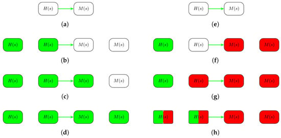
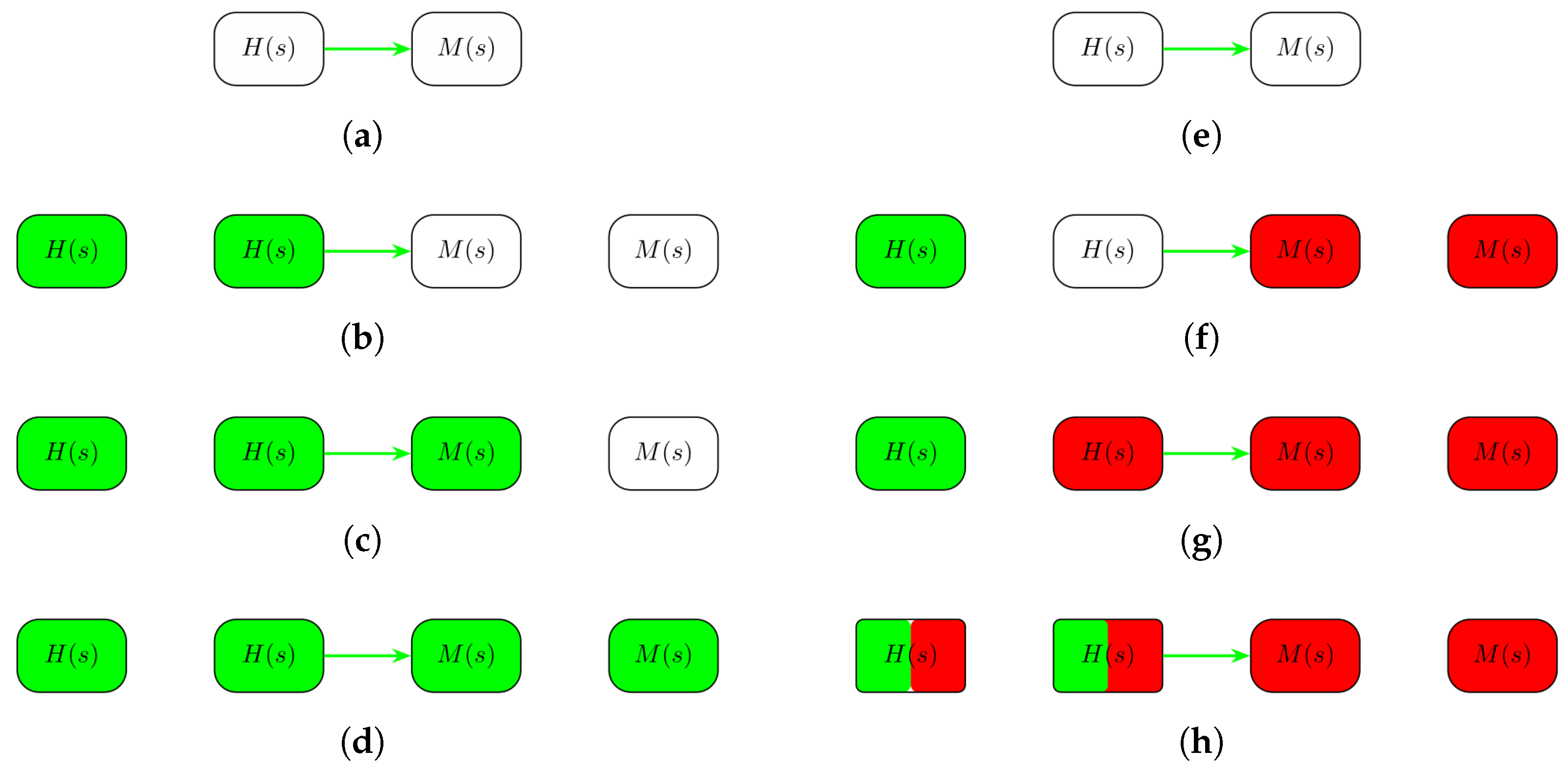
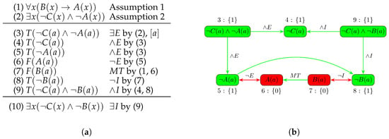
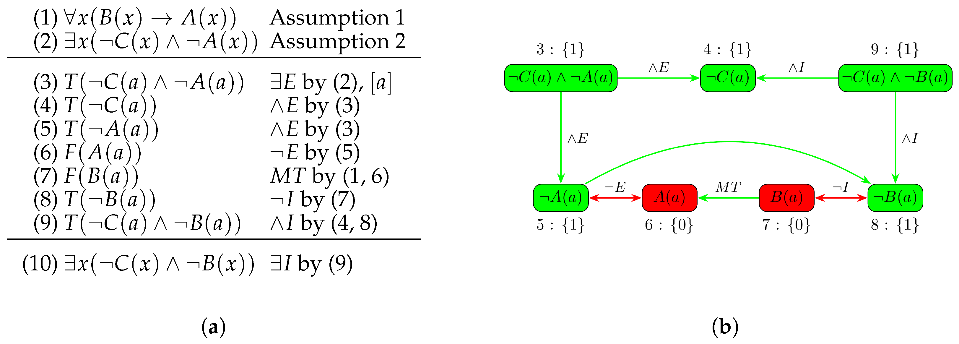
Disclaimer/Publisher’s Note: The statements, opinions and data contained in all publications are solely those of the individual author(s) and contributor(s) and not of MDPI and/or the editor(s). MDPI and/or the editor(s) disclaim responsibility for any injury to people or property resulting from any ideas, methods, instructions or products referred to in the content. |
© 2026 by the authors. Licensee MDPI, Basel, Switzerland. This article is an open access article distributed under the terms and conditions of the Creative Commons Attribution (CC BY) license.