Stability Conditions in Multiple-Input Multiple-Output Systems

Abstract

This paper investigates the stabilization of unstable third-order Multiple-Input Multiple-Output (MIMO) systems whose interaction structure is described by a doubly stochastic combined matrix, also known as the Relative Gain Array (RGA). Starting from systems with negative Niederlinski index, we derive necessary and sufficient conditions under which stability can be recovered through diagonal perturbations while preserving the doubly stochastic structure of the combined matrix. By exploiting the canonical representation of matrices associated with a prescribed combined matrix and the invariance properties under diagonal equivalence, the problem is reduced to a structured parametric form that allows a complete algebraic characterization. Special attention is given to perturbations involving the (1, 1) entry and one additional diagonal entry, leading to explicit bounds on the perturbation parameters that guarantee stabilization. The results extend previous papers on diagonal perturbations of combined matrices and provide a constructive method for stabilizing MIMO systems without altering their interaction pattern. Numerical examples illustrate the applicability of the proposed approach.

1. Introduction

The stability of Multiple-Input Multiple-Output (MIMO) systems is an important concept in control theory, systems engineering, industrial process control, and many other areas of engineering and applied science. Many industrial plants are operated using decentralized control architectures because of their simplicity, robustness, ease of maintenance, and low implementation cost [1,2]. In these settings, the stability and interaction structure among inputs and outputs play a crucial role in system performance and controller design. Typical examples include distillation columns, heat-exchanger networks, chemical reactors, and power systems, where significant interactions among control loops are unavoidable.

The Relative Gain Array (RGA) [3], also known in matrix-theoretic terms as the combined matrix, is an essential mathematical tool for analyzing multivariable systems in control engineering. From the work of [3,4], these indices have been extensively used in the analysis of industrial processes, where several manipulated and controlled variables interact through a coupled steady-state gain matrix. This matrix captures the steady-state coupling between inputs and outputs and provides valuable information for pairing decisions and decentralized control design. In particular, the sign of the Niederlinski index provides information regarding the feasibility of decentralized stabilization [5], while the RGA quantifies the degree of interaction among control loops. When the combined matrix is doubly stochastic, it represents a balanced interaction structure in which each input and output contributes uniformly. Preserving this property is often desirable in practical applications, as it reflects intrinsic symmetries and interaction patterns of the system. Several authors, including [6,7,8], have studied the specific algebraic and structural properties of combined and doubly stochastic matrices.

The stability of MIMO systems can be assessed through several criteria, among which the Niederlinski criterion plays a prominent role due to its simplicity and effectiveness [4]. This criterion relates stability to the sign of the Niederlinski index, which depends on the determinant of the system matrix and its diagonal entries. A negative index indicates instability, even when all individual loops are stable, highlighting the importance of interaction effects. From an engineering viewpoint, diagonal perturbations correspond to modifications of local loop dynamics while preserving the interaction structure among subsystems. Such perturbations naturally arise when retuning Proportional–Integral–Derivative (PID) controllers, adjusting valve gains, modifying local actuator sensitivities, or updating controller parameters after plant aging or operating-point changes.

Distillation columns constitute one of the most representative examples; reflux and boilup rates simultaneously affect tray temperatures and product compositions, leading to highly coupled MIMO systems. In such situations, negative Niederlinski indices may indicate difficulties in decentralized control design. Similar situations arise in heat-exchanger networks, where several flow rates influence multiple outlet temperatures simultaneously, and in continuously stirred tank reactors (CSTRs), where interactions between concentration and temperature control loops often generate coupled dynamics. Analogous problems appear in small-signal stability analysis of power systems, where local controller retuning modifies generator damping coefficients while transmission-network couplings remain essentially unchanged.

In practice, replacing the physical plant or modifying its interaction structure is often impossible or prohibitively expensive. Instead, engineers typically improve performance by retuning local controllers, modifying actuator gains, or adjusting damping coefficients, actions that can be mathematically interpreted as diagonal perturbations while preserving the underlying interaction pattern. This naturally raises the following question: under what conditions can stabilization be achieved through diagonal perturbations while maintaining the original interaction structure?

The present paper provides an answer to this question for a class of third-order systems with doubly stochastic combined matrices. In recent years, several works have investigated the interplay between combined matrices and stability properties, as well as the effect of structural transformations such as diagonal equivalence. In particular, diagonal perturbations have been proposed as a mechanism for modifying the properties of the system while preserving certain structural features [9].

This work is closely related to our previous study, where the role of the combined matrix and diagonal equivalence in the analysis of MIMO systems was investigated. While the methodology in both studies shares a similar theoretical foundation, a fundamental distinction in the present paper is the explicit incorporation of perturbations involving the $(1,1)$ entry together with an additional diagonal element. This specific setting prevents the direct use of the canonical matrix (where the $(1,1)$ entry is fixed to 1) and necessitates working directly with the general system matrix A, leading to a substantially more involved algebraic structure.

Consequently, the analysis cannot rely on the reduction techniques used in [9], and new explicit parametric conditions must be derived. This shift in perspective allows us to characterize, in a constructive and unified way, the admissible perturbation regions that simultaneously guarantee stabilization, through a sign change of the Niederlinski index, and preservation of the doubly stochastic interaction structure. In contrast to previous approaches, where either the perturbation mechanism or the structural constraints were more restrictive, the proposed paper provides explicit bounds for multiple perturbation patterns and extends the applicability of diagonal perturbation techniques to a broader class of structured MIMO systems.

The aim of this paper is to address this problem in the context of third-order MIMO systems. More precisely, we consider unstable systems whose combined matrix is doubly stochastic and investigate whether stability can be achieved through diagonal perturbations that preserve this property. We focus on perturbations involving the $(1,1)$ entry together with one additional diagonal entry. The obtained results extend [9].

The paper is organized as follows. Section 2 recalls the necessary definitions and known results on combined matrices and the Niederlinski criterion. Section 3 contains the main theoretical results on diagonal perturbations and stability conditions. Section 4 presents a numerical example illustrating the applicability of the proposed method. Finally, conclusions are discussed in Section 5.

2. Preliminaries and Known Results

In this section, we recall definitions and established theoretical results that will be used throughout the paper. To improve the structural clarity and readability of the manuscript, the key mathematical symbols and their corresponding engineering interpretations are summarized in

Table 1. Key notation and mathematical or engineering interpretation of symbols.

Symbol	Mathematical/Engineering Interpretation
A	Steady-state gain matrix of the MIMO proces.
$a_{ij}$	Entry of matrix A that representes the influence of input j on output i.
∘	Hadamard product; entrywise matrix multiplication.
$\mathcal{C}\left(A\right)$	Combined matrix; Relative Gain Array (RGA), quantifies loop interactions.
U	Doubly stochastic matrix, representing balanced interactions.
$NI\left[A\right]$	Niederlinski index. Structural indicator for stability.
T	Normalized representative of the system interaction structure.
$P\left(x\right)$	Polynomial defining canonical roots for the system.
$x_1,x_2$	Root of $P\left(x\right)$, parameter identifying the specific interaction pattern.
$A_p$	Perturbed system matrix after local adjustments.
$p_1,p_2\in \mathbb{R}$	Perturbed parameters; tuning parameters (PID gains, actuator sensitivities).
$a_{pij}^{\left(D\right)}$	Entries of $A_p^{\left(D\right)}=\mathcal{C}\left(A_p\right)\det \left(A_p\right)$. It is used to verify the structure.

.

Building upon the notation established in Table 1, we formally introduce the fundamental definitions and theoretical results that will be used throughout the paper, starting with the concept of the combined matrix.

Definition 1.

Let $A=\left(a_{ij}\right)\in {\mathbb{R}}^{n\times n}$ be a nonsingular matrix. The combined matrix of A, also known in control theory as the Relative Gain Array (RGA), is defined by

$$\mathcal{C}\left(A\right)=\left(c_{ij}\right)=A\circ A^{-T}$$

where ∘ means the Hadamard (entrywise) product. Equivalently,

$$c_{ij}={\displaystyle \frac{a_{ij}{A}_{ij}}{det\left(A\right)}},$$

where $A_{ij}$ is the cofactor of the $(i,j)$ entry of A.

Definition 2.

A real matrix $U=\left(u_{ij}\right)$ of order n is said to be doubly stochastic matrix if

$$u_{ij}\ge 0,{\displaystyle \sum _{i=1}^n}{u}_{ij}=1,\forall j=1,2,\dots ,n{\displaystyle \sum _{j=1}^n}{u}_{ij}=1,\forall i=1,2,\dots ,n.$$

It is well known that for any nonsingular matrix A, the rows and columns of $\mathcal{C}\left(A\right)$ sum to one; therefore, if $\mathcal{C}\left(A\right)$ is entrywise nonnegative, it is automatically doubly stochastic. Properties of combined matrices, including their invariance under diagonal equivalence and permutation similarity, can be found in [6].

Lemma 1.

The combined matrix $\mathcal{C}\left(A\right)=\left(c_{ij}\right)=A\circ A^{-T}$ of a nonsingular matrix $A=\left(a_{ij}\right)$ satisfies

(a) 

If $D_1$ and $D_2$ are two nonsingular diagonal matrices, then $\mathcal{C}\left(A\right)=\mathcal{C}\left(D_{1}A{D}_2\right)$.

(b) 

If P and Q are two permutation matrices, then $\mathcal{C}\left(PAQ\right)=P\mathcal{C}\left(A\right)Q$.

(c) 

$\mathcal{C}\left(A^{-T}\right)=\mathcal{C}\left(A\right)$.

In this paper, we focus on combined matrices of order 3. As shown in [6], if $U=\left(u_{ij}\right)$ is a doubly stochastic matrix of order 3 with no zero entries in its first row and first column, it can be written as

$$U=\left(\begin{array}{ccc}{u}_{11}& 1-u_{11}-u_{13}& u_{13}\\ 1-u_{11}-u_{31}& -1+u_{11}+u_{13}+u_{31}+u_{33}& 1-u_{13}-u_{33}\\ u_{31}& 1-u_{31}-u_{33}& u_{33}\end{array}\right).$$

(1)

There exists a nonsingular matrix A such that $\mathcal{C}\left(A\right)=U$ if and only if the polynomial

$$P\left(x\right)=u_{11}{x}^2+\left(u_{22}-u_{13}{u}_{31}-u_{33}{u}_{11}\right)x+u_{33}{u}_{13}{u}_{31}$$

has at least one real root distinct from $-{\displaystyle \frac{u_{13}{u}_{31}}{u_{21}+u_{31}}}$, with $u_{21}+u_{31}\ne 0$.

Following [6], each real root $x_i,i=1,2$ of $P\left(x\right)$ defines a canonical matrix $T_i$ of the form

$$T=\left(\begin{array}{ccc}1& 1& 1\\ 1& t_{22}& t_{23}\\ 1& t_{32}& t_{33}\end{array}\right),$$

(2)

where the entries can be expressed in terms of the matrix U given in (1),

$$\begin{array}{ccc}\hfill t_{22}& =& {\displaystyle \frac{u_{13}{u}_{31}+(-1+u_{13}+u_{31}+u_{33})x_i}{(u_{13}+x_i)(u_{31}+x_i)}}\hfill \\ \hfill t_{23}& =& {\displaystyle \frac{-1+u_{13}+u_{33}}{u_{13}+x_i}}\hfill \\ \hfill t_{32}& =& {\displaystyle \frac{-1+u_{31}+u_{33}}{u_{31}+x_i}}\hfill \\ \hfill t_{33}& =& {\displaystyle \frac{u_{33}}{x_i}}.\hfill \end{array}$$

It is well known that any matrix A satisfying $\mathcal{C}\left(A\right)=U$ is diagonally equivalent to one of these canonical matrices T, that is, $A=D_1^{-1}T{D}_2^{-1},$ where $D_1$ and $D_2$ are nonsingular diagonal matrices. By Lemma (1) we have $\mathcal{C}\left(A\right)=\mathcal{C}\left(T\right)$.

Throughout the paper, system stability refers to the closed-loop MIMO system associated with the system matrix under consideration. To ensure the stability of the system, we recall the Niederlinski criterion; see [4].

Theorem 1.

Consider a $2\times 2$ multivariable closed loop plant with $C\left(s\right)=\mathrm{diag}\{c_1\left(s\right),c_2\left(s\right)\}$. Also, assume that:

• $G\left(s\right)$ is stable.
• $P\left(s\right)=G\left(s\right)C\left(s\right)$ is a rational and proper matrix.
• All single-input single-output closed loops, obtained from a one-opening feedback loop, are stable.

• The system is unstable for all $k>0$ if and only if the Niederlinski index $NI\left[G\right(0\left)\right]<0$, being $NI\left[G\left(0\right)\right]={\displaystyle \frac{\det \left[G\right(0\left)\right]}{{\prod }_{i=1}^m{g}_{ii}\left(0\right)}}$.

The condition given in Theorem 1 is a sufficient condition for multivariable systems of size greater than or equal to 2.

3. Diagonal Perturbations and Stability Conditions

Without loss of generality, we focus on the root $x_1$ of the polynomial $P\left(x\right)$ and assume that the associated closed-loop MIMO system is unstable, that is, $NI\left[A\right]<0$. Throughout this section, system stability is characterized by the sign of the Niederlinski index associated with the system matrix A; consequently, the analysis of MIMO system stability is reduced to the study of algebraic properties of the matrix A. Moreover, the diagonal perturbations under consideration are restricted to those that preserve the doubly stochastic structure of the associated combined matrix.

Under these assumptions, we analyze how diagonal perturbations affect the entries of the canonical matrix $T=T_1$ corresponding to the root $x_1$, and we determine whether suitable perturbations can be used to recover system stability.

Theorem 2.

Let T be the nonsingular matrix given in (2) such that $C\left(T\right)=U$, where U is a doubly stochastic matrix of order 3, given in (1). Assume that the associated closed-loop MIMO system is unstable, that is, $NI\left[T\right]<0$. Then

$$\det \left(T\right)<0,t_{22}>0,t_{33}>0,\mathrm{and}{x}_1>0,$$

where $x_1$ is a root of the polynomial $P\left(x\right)$.

Proof. 

Since $NI\left[T\right]={\displaystyle \frac{\det \left(T\right)}{t_{22}{t}_{33}}}<0$, $\det \left(T\right)$ and the product $t_{22}{t}_{33}$ must have opposite signs. On the other hand, since $U=C\left(T\right)$ is doubly stochastic, its diagonal entries satisfy $u_{ii}>0$, which implies that the cofactors $T_{ii}$ have the same sign as $\det \left(T\right)$. In particular, this imposes compatibility conditions between the signs of $t_{22}$, $t_{33}$ and $\det \left(T\right)$.

We proceed by analyzing the possible sign configurations. If $\det \left(T\right)>0$, then $t_{22}{t}_{33}<0$, and $-1+u_{33}-x_1>0$ and $(u_{13}+x_1)(u_{31}+x_1)>0$ or $-1+u_{33}-x_1<0$ and $(u_{13}+x_1)(u_{31}+x_1)<0$. If $x_1>0$ then $u_{33}<1+x_1$, which implies $-1+u_{33}-x_1<0$, leading to a contradiction. If $x_1<0$, then $t_{33}={\displaystyle \frac{u_{33}}{x_1}}<0$. From the expression $u_{22}={\displaystyle \frac{t_{22}(t_{33}-1)}{\det \left(T\right)}}$, we obtain $t_{22}<0$, which gives $t_{22}{t}_{33}>0$ and it is a contradiction. Thus, if $\det \left(T\right)>0$, then $t_{22}{t}_{33}<0$, which contradicts the positivity constraints induced by the doubly stochastic structure of U.

Conversely, if $\det \left(T\right)<0$, then necessarily $t_{22}{t}_{33}>0$. Then $-1+u_{33}-x_1>0$ and $(u_{13}+x_1)(u_{31}+x_1)<0$ or $-1+u_{33}-x_1<0$ and $(u_{13}+x_1)(u_{31}+x_1)>0$. If $x_1<0$, then $t_{33}={\displaystyle \frac{u_{33}}{x_1}}<0$, which together with $u_{22}={\displaystyle \frac{t_{22}(t_{33}-1)}{\det \left(T\right)}}$ implies $t_{22}>0$ and $t_{22}{t}_{33}<0$ and it is a contradiction. If $x_1<0$ then $u_{33}>1+x_1$, and $-1+u_{33}-x_1<0$.

The expressions of the entries in terms of the root $x_1$ show that any admissible configuration requires $x_1>0$, which ensures that $t_{33}=u_{33}{x}_1>0$. Substituting this relation into the expression for $u_{22}$ yields $t_{22}>0$.

Therefore, the only admissible configuration compatible with instability and the doubly stochastic structure is $\det \left(T\right)<0$, $t_{22}>0$, $t_{33}>0$, and $x_1>0$. □

This work extends the results given in [9]. Thus, our start hypothesis is $NI\left[T\right]<0$ and we use the following result:

Theorem 3.

Let $T_i$, $i=1,2$ be matrices given in (2). $NI\left[T_i\right]<0$ and $U=\mathcal{C}\left(T_i\right)$ is a doubly stochastic matrix. Then,

$$NI\left[T_i\right]<0\mathrm{if}\mathrm{and}\mathrm{only}\mathrm{if}\det \left(T_i\right)<0,t_{22}>0,0<t_{33}<1,t_{23}<0,t_{32}<0,$$

(3)

being $t_{33}={\displaystyle \frac{u_{33}}{x_i}}$, $x_i>0$.

In this paper we use a perturbation in the entry $(1,1)$. This fact requires working directly with matrix $A=D_1^{-1}T{D}_2^{-1}$. We assume $x_1$ is a nonzero root of the polynomial $P\left(x\right)$ and, in this case, T is given by (2). Using $D_1^{-1}=\mathrm{diag}(1,a_{21}/a_{11},a_{31}/a_{11})$ and $D_2^{-1}=\mathrm{diag}(a_{11},a_{12},a_{13})$, we can write A as

$$A=\left(a_{ij}\right)=\left(\begin{array}{ccc}{a}_{11}& a_{12}& a_{13}\\ a_{21}& {\displaystyle \frac{a_{12}{a}_{21}{t}_{22}}{a_{11}}}& {\displaystyle \frac{a_{13}{a}_{21}{t}_{23}}{a_{11}}}\\ a_{31}& {\displaystyle \frac{a_{12}{a}_{31}{t}_{32}}{a_{11}}}& {\displaystyle \frac{a_{13}{a}_{31}{t}_{33}}{a_{11}}}\end{array}\right).$$

(4)

Using Lemma 1, $\mathcal{C}\left(A\right)=\mathcal{C}\left(T\right)=U$. We prove the relationship between the Niederlinski index of these matrices.

Lemma 2.

Let A be a nonsingular matrix given in (4) and let T be the matrix of order 3 with the structure given in (2). Then $NI\left[A\right]=NI\left[T\right]$.

Proof. 

By Theorem 1, $NI\left[A\right]={\displaystyle \frac{\det \left(A\right)}{{\prod }_{i=1}^m{a}_{ii}}}={\displaystyle \frac{\det \left(D_1^{-1}\right)\det \left(T\right)\det \left(D_2^{-1}\right)}{{\prod }_{i=1}^m{a}_{ii}}}={\displaystyle \frac{\det \left(T\right)}{t_{22}{t}_{33}}}.$ Thus, $NI\left[A\right]=NI\left[T\right]$. □

In the next result, we give the relationship between the matrices A and T.

Proposition 1.

Let T and A be nonsingular matrices given in (2) and (4). If $NI\left[A\right]<0$ and $\mathcal{C}\left(A\right)$ is a doubly stochastic matrix, then $t_{22}<1$ and $t_{22}{t}_{33}<t_{23}{t}_{32}$.

Proof. 

Using Lemma 1 and since $\{t_{22},t_{33}\}>0$ by (3), $\det \left(T\right)<0$. Since $\mathcal{C}\left(A\right)=U$ is doubly stochastic, all entries $c_{ij}\ge 0$ and $\det \left(T\right)<0$. Then, the entries of the following matrix must be nonpositive. This matrix is given by:

$$\mathcal{C}\left(A\right)\det \left(T\right)=\left(\begin{array}{ccc}{t}_{22}{t}_{33}-t_{23}{t}_{32}& t_{23}-t_{33}& t_{32}-t_{22}\\ t_{32}-t_{33}& t_{22}(t_{33}-1)& t_{23}-t_{23}{t}_{32}\\ t_{23}-t_{22}& t_{32}-t_{23}{t}_{32}& t_{33}(t_{22}-1)\end{array}\right).$$

From the entry $t_{33}(t_{22}-1)<0$, since $t_{33}>0$, we conclude $t_{22}\le 1$. Similarly, $t_{22}(t_{33}-1)<0$ implies $t_{33}\le 1$. Finally, $t_{22}{t}_{33}-t_{23}{t}_{32}<0$ yields the interaction bound $t_{22}{t}_{33}\le t_{23}{t}_{32}$. □

We suppose that our system is unstable. In the following result, we show how it affects the entries of the matrix A.

Proposition 2.

Let A be the matrix given in (4). If $NI\left[A\right]<0$ then

$$\det \left(A\right)a_{11}{a}_{12}{a}_{21}{a}_{13}{a}_{31}<0.$$

Proof. 

Using Lemma 2, we have $NI\left[A\right]=NI\left[T\right]$. By (3), the condition $NI\left[A\right]<0$ implies $t_{22}>0$ and $t_{33}>0$. From the structure of A we have

$${\displaystyle \prod _{i=1}^3}{a}_{ii}={\displaystyle \frac{a_{12}{a}_{21}{a}_{13}{a}_{31}}{a_{11}}}{t}_{22}{t}_{33}.$$

Thus,

$$NI\left[A\right]={\displaystyle \frac{\det \left(A\right)}{{\prod }_{i=1}^3{a}_{ii}}}={\displaystyle \frac{\det \left(A\right)a_{11}}{a_{12}{a}_{21}{a}_{13}{a}_{31}{t}_{22}{t}_{33}}}.$$

Since $t_{22}{t}_{33}>0$, it follows that $NI\left[A\right]<0$ if and only if $\det \left(A\right)$ and $a_{11}{a}_{12}{a}_{21}{a}_{13}{a}_{31}$ have opposite signs, which yields the stated alternatives. □

In [9] we analyzed diagonal perturbations of the $(2,2)$ and $(3,3)$ entries of the matrix T. Here, we focus on perturbations acting on the $(1,1)$ entry and one other diagonal entry of the matrix A. Moreover, we restrict our study to perturbations for which the combined matrix $\mathcal{C}\left(A_p\right)$ remains doubly stochastic.

3.1. Case $\det \left(A\right)<0$ and $a_{11}{a}_{12}{a}_{21}{a}_{13}{a}_{31}>0$

We choose a pattern, and for this study we select this one as a reference case, $a_{11}<0$, $a_{12}<0$, $a_{13}<0$, $a_{21}>0$ and $a_{31}<0$. We begin our analysis by applying diagonal perturbations to the entries $a_{11}$ and $a_{22}$, obtaining the matrix $A_P=A+\mathrm{diag}(p_1,p_2,0)$ which has the following structure

$$A_P=\left(a{p}_{ij}\right)=\left(\begin{array}{ccc}{a}_{11}+p_1& a_{12}& a_{13}\\ a_{21}& {\displaystyle \frac{a_{12}{a}_{21}{t}_{22}}{a_{11}}}+p_2& {\displaystyle \frac{a_{13}{a}_{21}{t}_{23}}{a_{11}}}\\ a_{31}& {\displaystyle \frac{a_{12}{a}_{31}{t}_{32}}{a_{11}}}& {\displaystyle \frac{a_{13}{a}_{31}{t}_{33}}{a_{11}}}\end{array}\right),$$

(5)

with $p_1,p_2\in \mathrm{R}$ and $p_1,p_2>0$.

Remark 1.

The choice of perturbing the $(1,1)$ entry alongside one additional diagonal entry is motivated by both technical and comparative requirements. First, rank-1 perturbations are insufficient to satisfy the initial stabilization conditions while preserving the doubly stochastic structure. Second, while higher-rank perturbations could be considered, they significantly reduce the degrees of freedom available to derive the explicit analytical bounds presented here. This structure extends the work established in [9], allowing for a direct comparison with previous stabilization results.

Using this matrix, we establish the following result.

Theorem 4.

Let $A=\left(a_{ij}\right)$ be the matrix given in (4) such that $NI\left[A\right]<0$ and let $U=\mathcal{C}\left(A\right)$ be a doubly stochastic matrix. Consider the perturbed matrix $A_p=A+\mathrm{diag}(p_1,p_2,0)$, defined in (5), with $p_1,p_2\in \mathrm{R},p_1,p_2>0$. If the parameters $p_1$ and $p_2$ satisfy $\det \left(A_p\right)<0$, $a_{11}+p_1>0$ and

$$-a_{11}<p_1<min\left\{{\displaystyle \frac{a_{11}(1-t_{32})}{t_{32}}},{\displaystyle \frac{a_{11}(1-t_{23})}{t_{23}}}\right\},{\displaystyle \frac{a_{12}{a}_{21}(t_{23}{t}_{32}-t_{22}{t}_{33})}{a_{11}{t}_{33}}}<p_2,$$

then $A_p$ satisfies $NI\left[A_p\right]>0$ and $\mathcal{C}\left(A_p\right)$ remains doubly stochastic.

Proof. 

The proof is structured in two steps, corresponding to the stabilization condition and the preservation of the interaction structure.

Step 1: Niederlinski Index:

A direct computation shows that the determinant of the perturbed matrix can be written as

$$\det \left(A_p\right)={\displaystyle \frac{a_{13}{a}_{31}}{a_{11}^2}}N(p_1,p_2),$$

(6)

where

$$N(p_1,p_2)=\left(a_{11}{a}_{12}{a}_{21}d+a_{11}^2{p}_2(t_{33}-1)+a_{11}{p}_1{p}_2{t}_{33}+a_{12}{a}_{21}{p}_1(-t_{23}{t}_{32}+t_{22}{t}_{33})\right).$$

(7)

Under the hypothesis $\det \left(A_p\right)<0$ and the positivity of $a_{13}{a}_{31}/a_{11}^2$, it follows that $N(p_1,p_2)<0$. The perturbed Niederlinski index can be factorized as

$$NI\left[A_p\right]={\displaystyle \frac{N(p_1,p_2)}{(a_{11}+p_1)(a_{11}{p}_2+a_{12}{a}_{21}{t}_{22})t_{33}}}.$$

Since $NI\left[T\right]=NI\left[A\right]<0$, the relations given in (3) hold. Furthermore, the specific sign pattern selected for this case implies that $a_{13}{a}_{31}>0$ and $a_{12}{a}_{21}<0$. Since $t_{33}>0$ and $N(p_1,p_2)<0$, the condition $NI\left[A_p\right]>0$ is equivalent to

$$(a_{11}+p_1)(a_{11}{p}_2+a_{12}{a}_{21}{t}_{22})<0.$$

Using that $p_2>0$, $t_{22}>0$, and $a_{12}{a}_{21}<0$, we have $a_{11}{p}_2+a_{12}{a}_{21}{t}_{22}<0$. By hypothesis $a_{11}+p_1>0$, then $NI\left[A_p\right]>0$.

Step 2: Doubly stochastic structure:

Since $\det \left(A_p\right)<0$, to demonstrate that $\mathcal{C}\left(A_p\right)$ is doubly stochastic is equivalent to requiring that all entries of $A_p^{\left(D\right)}$ are negative, being $A_p^{\left(D\right)}=\left(a_{pij}^{\left(D\right)}\right)=\mathcal{C}\left(A_p\right)\det \left(A_p\right)$.

• Entry $a_{p11}^{\left(D\right)}$. A direct computation yields:

  $$a_{p11}^{\left(D\right)}={\displaystyle \frac{a_{13}{a}_{31}(a_{11}+p_1)}{a_{11}^2}}\left(a_{11}{p}_2{t}_{33}+a_{12}{a}_{21}(-t_{23}{t}_{32}+t_{22}{t}_{33})\right).$$
  Since $a_{13}{a}_{31}>0$, $a_{11}+p_1>0$, and by hypothesis $p_2>{\displaystyle \frac{a_{12}{a}_{21}(t_{23}{t}_{32}-t_{22}{t}_{33})}{a_{11}{t}_{33}}}$, we obtain $a_{11}{p}_2{t}_{33}+a_{12}{a}_{21}(-t_{23}{t}_{32}+t_{22}{t}_{33})<0$. Hence, $a_{p11}^{\left(D\right)}$ is negative.
• The following entries are negative due to the doubly stochastic structure of $\mathcal{C}\left(A\right)$ and the sign $t_{23}<0$, $t_{32}<0$.

  $$\begin{array}{ccc}\hfill a_{p12}^{\left(D\right)}& =& {\displaystyle \frac{a_{12}{a}_{13}{a}_{21}{a}_{31}(t_{23}-t_{33})}{a_{11}}}\hfill \\ \hfill a_{p13}^{\left(D\right)}& =& -{\displaystyle \frac{a_{13}{a}_{31}(a_{11}{p}_2+a_{12}{a}_{21}(t_{22}-t_{32})}{a_{11}}}\hfill \\ \hfill a_{p21}^{\left(D\right)}& =& {\displaystyle \frac{a_{12}{a}_{13}{a}_{21}{a}_{31}(t_{32}-t_{33})}{a_{11}}}\hfill \\ \hfill a_{p31}^{\left(D\right)}& =& -{\displaystyle \frac{a_{13}{a}_{31}(a_{11}{p}_2+a_{12}{a}_{21}(t_{22}-t_{23})}{a_{11}}}.\hfill \end{array}$$
• Entry $a_{p22}^{\left(D\right)}$. Using the hypothesis, we obtain

  $$a_{p22}^{\left(D\right)}={\displaystyle \frac{a_{13}{a}_{31}(a_{11}{p}_2+a_{12}{a}_{21}{t}_{22})}{a_{11}^2}}\left(a_{11}(-1+t_{33})+p_1{t}_{33}\right)<0.$$
• The following entries are negative provided that $p_1<{\displaystyle \frac{a_{11}(1-t_{32})}{t_{32}}}$ and $p_1<{\displaystyle \frac{a_{11}(1-t_{23})}{t_{23}}}$, respectively, as defined by the hypothesis.

  $$\begin{array}{ccc}\hfill a_{p23}^{\left(D\right)}& =& -{\displaystyle \frac{a_{12}{a}_{13}{a}_{21}{a}_{31}{t}_{23}(a_{11}(-1+t_{32})+p_1{t}_{32})}{a_{11}^2}}\hfill \\ \hfill a_{p32}^{\left(D\right)}& =& -{\displaystyle \frac{a_{12}{a}_{13}{a}_{21}{a}_{31}(a_{11}(-1+t_{23})+p_1{t}_{23})t_{32}}{a_{11}^2}}.\hfill \end{array}$$
• Entry $a_{p33}^{\left(D\right)}$ is negative based on the hypothesis

  $$a_{p33}^{\left(D\right)}={\displaystyle \frac{a_{13}{a}_{31}(a_{11}^2{p}_2+a_{11}{p}_1{p}_2+a_{11}{a}_{12}{a}_{21}(-1+t_{22})+a_{12}{a}_{21}{p}_1{t}_{22})t_{33}}{a_{11}^2}}.$$

As all entries $a_{pij}^{\left(D\right)}<0$ and $\det \left(A_p\right)<0$, the matrix $\mathcal{C}\left(A_p\right)$ is doubly stochastic. □

The proof of Theorem 4 illustrates the general mechanism underlying all admissible perturbation patterns. Stabilization is governed by the sign of the perturbation polynomial $N(p_1,p_2)$, while the preservation of the doubly stochastic structure is ensured by maintaining a consistent sign between the cofactors $a_{pij}^{\left(D\right)}$ and the determinant of $A_p$.

Although each perturbation configuration leads to different algebraic expressions, the structure of the analysis remains essentially the same. In particular, all cases can be treated by combining a factorization of the perturbed determinant, a sign analysis of the Niederlinski index, and a verification that the cofactors preserve the required sign pattern.

To avoid repetitive computations, the sign conditions required for each perturbation pattern are summarized in

Table 2. Summary of admissible diagonal perturbation patterns ensuring stabilization and preservation of the doubly stochastic structure.

Result	Perturbation	$\mathbf{sign}\left(\mathbf{det}\left({\mathit{A}}_{\mathit{p}}\right)\right)$	Required Sign
Theorem 4	$A+\mathrm{diag}(p_1,p_2,0)$	−	$a_{pij}^{\left(D\right)}<0$
Proposition 3	$A+\mathrm{diag}(-p_1,-p_2,0)$	−	$a_{pij}^{\left(D\right)}<0$
Proposition 4	$A+\mathrm{diag}(p_1,0,-p_2)$	−	$a_{pij}^{\left(D\right)}<0$
Proposition 5	$A+\mathrm{diag}(-p_1,0,p_2)$	−	$a_{pij}^{\left(D\right)}<0$
Proposition 6	$A+\mathrm{diag}(p_1,-p_2,0)$	+	$a_{pij}^{\left(D\right)}>0$
Proposition 7	$A+\mathrm{diag}(-p_1,p_2,0)$	+	$a_{pij}^{\left(D\right)}>0$
Proposition 8	$A+\mathrm{diag}(p_1,0,-p_2)$	+	$a_{pij}^{\left(D\right)}>0$
Proposition 9	$A+\mathrm{diag}(-p_1,0,p_2)$	+	$a_{pij}^{\left(D\right)}>0$

. These conditions provide a unified characterization of all admissible perturbations ensuring stabilization and preservation of the interaction structure.

The remaining perturbation cases are stated below. Their proofs follow the same algebraic technique as in Theorem 4 and are therefore omitted for conciseness and we briefly indicate the key arguments. For completeness, we add the proofs to Appendix A. Now, we apply perturbations to the entries $a_{11}$ and $a_{22}$, obtaining the perturbed matrix $A_P=A+\mathrm{diag}(-p_1,-p_2,0)$.

Proposition 3.

Let $A=\left(a_{ij}\right)$ be the matrix given in (4) such that $NI\left[A\right]<0$ and let $U=\mathcal{C}\left(A\right)$ be a doubly stochastic matrix. Consider the perturbed matrix $A_p=A+\mathrm{diag}(-p_1,-p_2,0)$, with the same structure as in (5), with $p_1,p_2\in \mathrm{R},p_1,p_2>0$. If $\det \left(A_p\right)<0$ and

$${\displaystyle \frac{a_{11}(t_{33}-1)}{t_{33}}}<p_1,{\displaystyle \frac{a_{12}{a}_{21}{t}_{22}}{a_{11}}}<p_2<min\left\{{\displaystyle \frac{a_{12}{a}_{21}(t_{22}-t_{32})}{a_{11}}},{\displaystyle \frac{a_{12}{a}_{21}(t_{22}-t_{23})}{a_{11}}}\right\},$$

then $A_p$ satisfies $NI\left[A_p\right]>0$ and $\mathcal{C}\left(A_p\right)$ is doubly stochastic.

Proof. 

The determinant of the perturbed matrix admits a factorization of the form $\det \left(A_p\right)=\alpha N(p_1,p_2)$, where the coefficient $\alpha$ has a fixed sign under the proposed perturbation pattern. The imposed bounds on $p_1$ and $p_2$ ensure that $N(p_1,p_2)>0$, while the denominator of $NI\left[A_p\right]$ remains positive, yielding $NI\left[A_p\right]>0$.

Moreover, as summarized in Table 2, the same bounds guarantee that all cofactors $a_{pij}^{\left(D\right)}$ preserve the sign of $\det \left(A_p\right)$. Consequently, the combined matrix $\mathcal{C}\left(A_p\right)$ remains doubly stochastic. □

Next, the perturbations are applied to $a_{11}$ and $a_{33}$, obtaining the matrix $A_P=A+\mathrm{diag}(p_1,0,-p_2)$.

Proposition 4.

Let $A=\left(a_{ij}\right)$ be the matrix given in (4) such that $NI\left[A\right]<0$ and let $U=\mathcal{C}\left(A\right)$ be a doubly stochastic matrix. Consider the perturbed matrix $A_p=A+\mathrm{diag}(p_1,0,-p_2)$, with the same structure as in (5), with $p_1,p_2\in \mathrm{R},p_1,p_2>0$. If $\det \left(A_p\right)<0$, $a_{11}+p_1>0$ and

$$-a_{11}<p_1<min\left\{{\displaystyle \frac{a_{11}(1-t_{23})}{t_{23}}},{\displaystyle \frac{a_{11}(1-t_{32})}{t_{32}}}\right\},{\displaystyle \frac{a_{13}{a}_{31}(t_{22}{t}_{33}-t_{23}{t}_{32})}{a_{11}{t}_{22}}}<p_2,$$

then $A_p$ satisfies $NI\left[A_p\right]>0$ and $\mathcal{C}\left(A_p\right)$ is doubly stochastic.

Proof. 

For this perturbation pattern, the determinant of $A_p$ can be written as $\det \left(A_p\right)=\alpha N(p_1,p_2)$, where $\alpha$ has a fixed sign. The imposed lower bound on $p_2$ ensures that $N(p_1,p_2)<0$, and hence $\det \left(A_p\right)<0$.

The Niederlinski index can be factorized into three terms, whose signs are determined by the sign pattern of the original matrix and the condition $a_{11}+p_1>0$. The bound on $p_2$ guarantees that the third factor is negative, which implies $NI\left[A_p\right]>0$.

Finally, the upper bounds on $p_1$ ensure that all interaction cofactors retain their original sign, while the diagonal cofactors remain consistent with $\det \left(A_p\right)$. Therefore, the combined matrix remains doubly stochastic. □

Finally, if the perturbations are applied to $a_{11}$ and $a_{33}$, we obtain the matrix $A_P=A+\mathrm{diag}(-p_1,0,p_2)$ and we show this in the following result.

Proposition 5.

Let $A=\left(a_{ij}\right)$ be the matrix given in (4) such that $NI\left[A\right]<0$ and let $U=\mathcal{C}\left(A\right)$ be a doubly stochastic matrix. Consider the perturbed matrix $A_p=A+\mathrm{diag}(-p_1,0,p_2)$, with the same structure as in (5), with $p_1,p_2\in \mathrm{R},p_1,p_2>0$. If $\det \left(A_p\right)<0$ and

$${\displaystyle \frac{a_{11}(t_{22}-1)}{t_{22}}}<p_1,{\displaystyle \frac{-a_{13}{a}_{31}{t}_{33}}{a_{11}}}<p_2<min\left\{{\displaystyle \frac{-a_{13}{a}_{31}(t_{33}-t_{23})}{a_{11}}},{\displaystyle \frac{-a_{13}{a}_{31}(t_{33}-t_{32})}{a_{11}}}\right\},$$

then $A_p$ satisfies $NI\left[A_p\right]>0$ and $\mathcal{C}\left(A_p\right)$ is doubly stochastic.

Proof. 

This perturbation pattern differs from that of Proposition 4 only by the sign of $p_1$, while the algebraic structure of the determinant and the associated perturbation polynomial remains unchanged.

By applying the transformation from $p_1$ to $-p_1$, the analysis reduces to the technique of Proposition 4, with the corresponding inversion of the sign conditions. The bounds on $p_1$ and $p_2$ are precisely those required to preserve the sign of the perturbation polynomial and ensure that the denominator of the Niederlinski index has the appropriate sign.

The preservation of the doubly stochastic structure follows from the same cofactor sign conditions, which remain invariant under this transformation. □

3.2. Case $\det \left(A\right)>0$ and $a_{11}{a}_{12}{a}_{21}{a}_{13}{a}_{31}<0$

We choose a pattern, and for this study we select this one as a reference case, $a_{11}<0$, $a_{12}<0$, $a_{13}<0$, $a_{21}<0$ and $a_{31}<0$. Since the technique is the same as the previous subsection, we show only the obtained results. We begin our analysis by applying diagonal perturbations to the entries $a_{11}$ and $a_{22}$, obtaining the matrix $A_P=A+\mathrm{diag}(p_1,-p_2,0)$.

Proposition 6.

Let $A=\left(a_{ij}\right)$ be the matrix given in (4) such that $NI\left[A\right]<0$ and let $U=\mathcal{C}\left(A\right)$ be a doubly stochastic matrix. Consider the perturbed matrix $A_p=A+\mathrm{diag}(p_1,-p_2,0)$, with the same structure as in (5), with $p_1,p_2\in \mathrm{R},p_1,p_2>0$. If $\det \left(A_p\right)>0$, $a_{11}+p_1>0$ and

$$-a_{11}<p_1<min\left\{{\displaystyle \frac{a_{11}(1-t_{23})}{t_{23}}},{\displaystyle \frac{a_{11}(1-t_{32})}{t_{32}}}\right\},{\displaystyle \frac{-a_{12}{a}_{21}(t_{23}{t}_{32}-t_{22}{t}_{33})}{a_{11}{t}_{33}}}<p_2,$$

then $A_p$ satisfies $NI\left[A_p\right]>0$ and $\mathcal{C}\left(A_p\right)$ is doubly stochastic.

Proof. 

In this configuration, the determinant of the perturbed matrix changes sign with respect to the previous case, i.e., $\det \left(A_p\right)>0$. Consequently, the preservation of the doubly stochastic structure requires all cofactors to be positive instead of negative.

The perturbation polynomial $N(p_1,p_2)$ retains the same structure as in Theorem 4, and the imposed bounds ensure that its sign is compatible with $\det \left(A_p\right)>0$, yielding $NI\left[A_p\right]>0$.

The cofactor conditions are obtained by reversing the sign constraints in Table 2, which guarantees that $\mathcal{C}\left(A_p\right)$ remains entrywise nonnegative. □

Next, the perturbations are applied to $a_{11}$ and $a_{22}$, thus obtaining the matrix $A_P=A+\mathrm{diag}(-p_1,p_2,0)$.

Proposition 7.

Let $A=\left(a_{ij}\right)$ be the matrix given in (4) such that $NI\left[A\right]<0$ and let $U=\mathcal{C}\left(A\right)$ be a doubly stochastic matrix. Consider the perturbed matrix $A_p=A+\mathrm{diag}(-p_1,p_2,0)$, with the same structure as in (5), with $p_1,p_2\in \mathrm{R},p_1,p_2>0$. If $\det \left(A_p\right)>0$ and

$${\displaystyle \frac{a_{11}(t_{33}-1)}{t_{33}}}<p_1,{\displaystyle \frac{-a_{12}{a}_{21}{t}_{22}}{a_{11}}}<p_2<min\left\{{\displaystyle \frac{-a_{12}{a}_{21}(t_{22}-t_{23})}{a_{11}}},{\displaystyle \frac{-a_{12}{a}_{21}(t_{22}-t_{32})}{a_{11}}}\right\},$$

then $A_p$ satisfies $NI\left[A_p\right]>0$ and $\mathcal{C}\left(A_p\right)$ is doubly stochastic.

Proof. 

This case can be interpreted as the symmetric counterpart of Proposition 6 with respect to the perturbation direction. The determinant remains positive, and the perturbation polynomial $N(p_1,p_2)$ satisfies analogous sign conditions under the proposed bounds.

The sign of the denominator of $NI\left[A_p\right]$ is determined by the factor $(a_{11}-p_1)$, whose negativity is enforced by the lower bound on $p_1$. Together with the sign of $N(p_1,p_2)$, this yields $NI\left[A_p\right]>0$.

The preservation of the doubly stochastic structure follows from the same cofactor conditions, which are consistent with $\det \left(A_p\right)>0$. □

If the perturbations are applied to $a_{11}$ and $a_{33}$, we obtain the matrix $A_P=A+\mathrm{diag}(p_1,0,-p_2)$ along with the following result.

Proposition 8.

Let $A=\left(a_{ij}\right)$ be the matrix given in (4) such that $NI\left[A\right]<0$ and let $U=\mathcal{C}\left(A\right)$ be a doubly stochastic matrix. Consider the perturbed matrix $A_p=A+\mathrm{diag}(p_1,0,-p_2)$, with the same structure as in (5), with $p_1,p_2\in \mathrm{R},p_1,p_2>0$. If $\det \left(A_p\right)>0$, $a_{11}+p_1>0$ and

$$-a_{11}<p_1<min\left\{{\displaystyle \frac{a_{11}(1-t_{23})}{t_{23}}},{\displaystyle \frac{a_{11}(1-t_{32})}{t_{32}}}\right\},{\displaystyle \frac{a_{13}{a}_{31}(-t_{23}{t}_{32}+t_{22}{t}_{33})}{a_{11}{t}_{22}}}<p_2,$$

then $A_p$ satisfies $NI\left[A_p\right]>0$ and $\mathcal{C}\left(A_p\right)$ is doubly stochastic.

Proof. 

The determinant of the perturbed matrix admits a factorization in terms of the perturbation polynomial $N(p_1,p_2)$, whose sign is controlled by the imposed bounds on $p_2$. These conditions ensure that $\det \left(A_p\right)>0$.

The Niederlinski index is expressed as a product of three factors, and the corresponding bounds guarantee that their combined sign is positive, yielding $NI\left[A_p\right]>0$.

The sign of each cofactor follows from the same inequalities defining the admissible region. In particular, the bounds on $p_1$ prevent any sign change in the interaction terms, ensuring that the combined matrix remains doubly stochastic. □

Finally, if the perturbations are applied to $a_{11}$ and $a_{33}$, we obtain the matrix $A_P=A+\mathrm{diag}(-p_1,0,p_2)$ along with the following result.

Proposition 9.

Let $A=\left(a_{ij}\right)$ be the matrix given in (4) such that $NI\left[A\right]<0$ and let $U=\mathcal{C}\left(A\right)$ be a doubly stochastic matrix. Consider the perturbed matrix $A_p=A+\mathrm{diag}(-p_1,0,p_2)$, with the same structure as in (5), with $p_1,p_2\in \mathrm{R},p_1,p_2>0$. If $\det \left(A_p\right)>0$ and

$${\displaystyle \frac{a_{11}(t_{22}-1)}{t_{22}}}<p_1{\displaystyle \frac{-a_{13}{a}_{31}{t}_{33}}{a_{11}}}<p_2<min\left\{{\displaystyle \frac{-a_{13}{a}_{31}(t_{33}-t_{32})}{a_{11}}},{\displaystyle \frac{-a_{13}{a}_{31}(t_{33}-t_{23})}{a_{11}}}\right\},$$

then $A_p$ satisfies $NI\left[A_p\right]>0$ and $\mathcal{C}\left(A_p\right)$ is doubly stochastic.

Proof. 

This configuration completes the set of admissible perturbation patterns. The determinant remains positive and can be expressed as a scaled version of the perturbation polynomial $N(p_1,p_2)$.

The bounds on $p_1$ and $p_2$ ensure that the numerator and denominator of $NI\left[A_p\right]$ have compatible signs, yielding $NI\left[A_p\right]>0$. Moreover, the same bounds guarantee that all cofactors preserve the sign required by $\det \left(A_p\right)>0$.

Therefore, this case satisfies stabilization and structure-preserving conditions. □

The results presented in this section provide a complete characterization of diagonal perturbations that achieve stabilization while preserving the interaction structure. The explicit bounds obtained for each perturbation pattern define admissible regions in the parameter space $(p_1,p_2)$, thereby offering a constructive method for structure-preserving stabilization of MIMO systems.

4. Applied Examples

In this section, we illustrate the theoretical results obtained in previous sections through numerical examples. The purpose is to show how diagonal perturbations can modify the sign of the Niederlinski index while preserving the doubly stochastic structure of the combined matrix.

We consider the matrix T, encoding the interaction structure of the system, and construct a system matrix A that is diagonally equivalent to T.

$$T=\left(\begin{array}{ccc}1& 1& 1\\ 1& 0.0742& -1.9627\\ 1& -2.4719& 0.8900\end{array}\right).$$

This matrix satifies $NI\left[T\right]=-154.2861<0$ and $\det \left(T\right)=-10.1842<0$ and its associated combined matrix is doubly stochastic.

$$\mathcal{C}\left(T\right)=\left(\begin{array}{ccc}0.4699& 0.2801& 0.2500\\ 0.3301& 0.0008& 0.6691\\ 0.2000& 0.7191& 0.0809\end{array}\right).$$

Following the construction described in Section 2, we define diagonal matrices $D_1^{-1}=\mathrm{diag}\left(1,{\displaystyle \frac{a_{21}}{a_{11}}},{\displaystyle \frac{a_{31}}{a_{11}}}\right)$, $D_2^{-1}=\mathrm{diag}(a_{11},a_{12},a_{13})$, and construct the system matrix $A=D_1^{-1}T{D}_2^{-1}$, which preserves the combined matrix structure, i.e., $\mathcal{C}\left(A\right)=\mathcal{C}\left(T\right)$.

4.1. Case $\det \left(A\right)<0$

We select the parameters $a_{11}=-1$, $a_{12}=-2$, $a_{13}=-3$, $a_{21}=1$, $a_{31}=-5$. The resulting matrix is

$$A=\left(\begin{array}{ccc}\hfill -1& \hfill -2& \hfill -3\\ \hfill 1& \hfill 0.1483& \hfill -5.8880\\ \hfill -5& \hfill 24.7188& \hfill -13.3500\end{array}\right).$$

A direct computation shows that $\det \left(A\right)=-305.5250<0$. By Lemma 2, $NI\left[A\right]=NI\left[T\right]=-154.2861<0$, so the system is unstable.

We now apply a diagonal perturbation of the form $A_p=A+\mathrm{diag}(p_1,p_2,0)$. According to Theorem 4, stability is ensured if

$$0<p_1<min\left\{1.4046,1.5095\right\},10.7538<p_2,$$

For instance, choosing $p_1=1.3$, $p_2=10.8$, we obtain a perturbed matrix $A_p$ such that $NI\left[A_p\right]=7.3925>0$ and $\mathcal{C}\left(A_p\right)$ remains doubly stochastic

$$A_p=\left(\begin{array}{ccc}0.3000& -2.0000& -3.0000\\ 1.0000& 10.9483& -5.8880\\ -5.0000& 24.7188& -13.3500\end{array}\right),\mathcal{C}\left(A_p\right)=\left(\begin{array}{ccc}0.0006& 0.2640& 0.7354\\ 0.3111& 0.6419& 0.0469\\ 0.6883& 0.0941& 0.2176\end{array}\right)$$

Thus, the system becomes stable without altering the interaction structure.

We now apply a diagonal perturbation of the form $A_p=A+\mathrm{diag}(p_1,0,-p_2)$. According to Proposition 4, stability is ensured if

$$1<p_1<1.4046,967.8455<p_2,$$

For instance, choosing $p_1=1.3$, $p_2=968$, we obtain a perturbed matrix $A_p$ such that $NI\left[A_p\right]=48.0519>0$ and $\mathcal{C}\left(A_p\right)$ remains doubly stochastic

$$A_p=\left(\begin{array}{ccc}0.3000& -2.0000& -3.0000\\ 1.0000& 0.1483& -5.8880\\ -5.0000& 24.7188& -981.3500\end{array}\right),\mathcal{C}\left(A_p\right)=\left(\begin{array}{ccc}0& 0.9636& 0.0364\\ 0.9709& 0.0219& 0.0073\\ 0.0291& 0.0145& 0.9563\end{array}\right)$$

Thus, the system becomes stable without altering the interaction structure.

4.2. Case $\det \left(A\right)>0$

To illustrate a different sign pattern, we modify the previous system by setting $a_{21}=-1$. The resulting matrix becomes

$$A=\left(\begin{array}{ccc}-1& -2& -3\\ -1& -0.1483& 5.8880\\ -5& 24.7188& -13.3500\end{array}\right).$$

A direct computation shows that $\det \left(A\right)=305.5254>0$. By Lemma 2, $NI\left[A\right]=NI\left[T\right]=-154.2861<0$, so the system is unstable.

We now apply a diagonal perturbation of the form $A_p=A+\mathrm{diag}(p_1,-p_2,0)$. According to Proposition 6, stability is ensured if

$$1<p_1<1.4046,10.7538<p_2,$$

For instance, choosing $p_1=1.3$, $p_2=10.8$, we obtain a perturbed matrix $A_p$ such that $NI\left[A_p\right]=7.3925>0$ and $\mathcal{C}\left(A_p\right)$ remains doubly stochastic

$$A_p=\left(\begin{array}{ccc}0.3000& -2.0000& -3.0000\\ -1.0000& -10.9483& 5.8880\\ -5.0000& 24.7188& -13.3500\end{array}\right),\mathcal{C}\left(A_p\right)=\left(\begin{array}{ccc}0.0006& 0.2640& 0.7354\\ 0.3111& 0.6419& 0.0469\\ 0.6883& 0.0941& 0.2176\end{array}\right)$$

Thus, the system becomes stable without altering the interaction structure.

4.3. Comparative Analysis of Perturbation Strategies

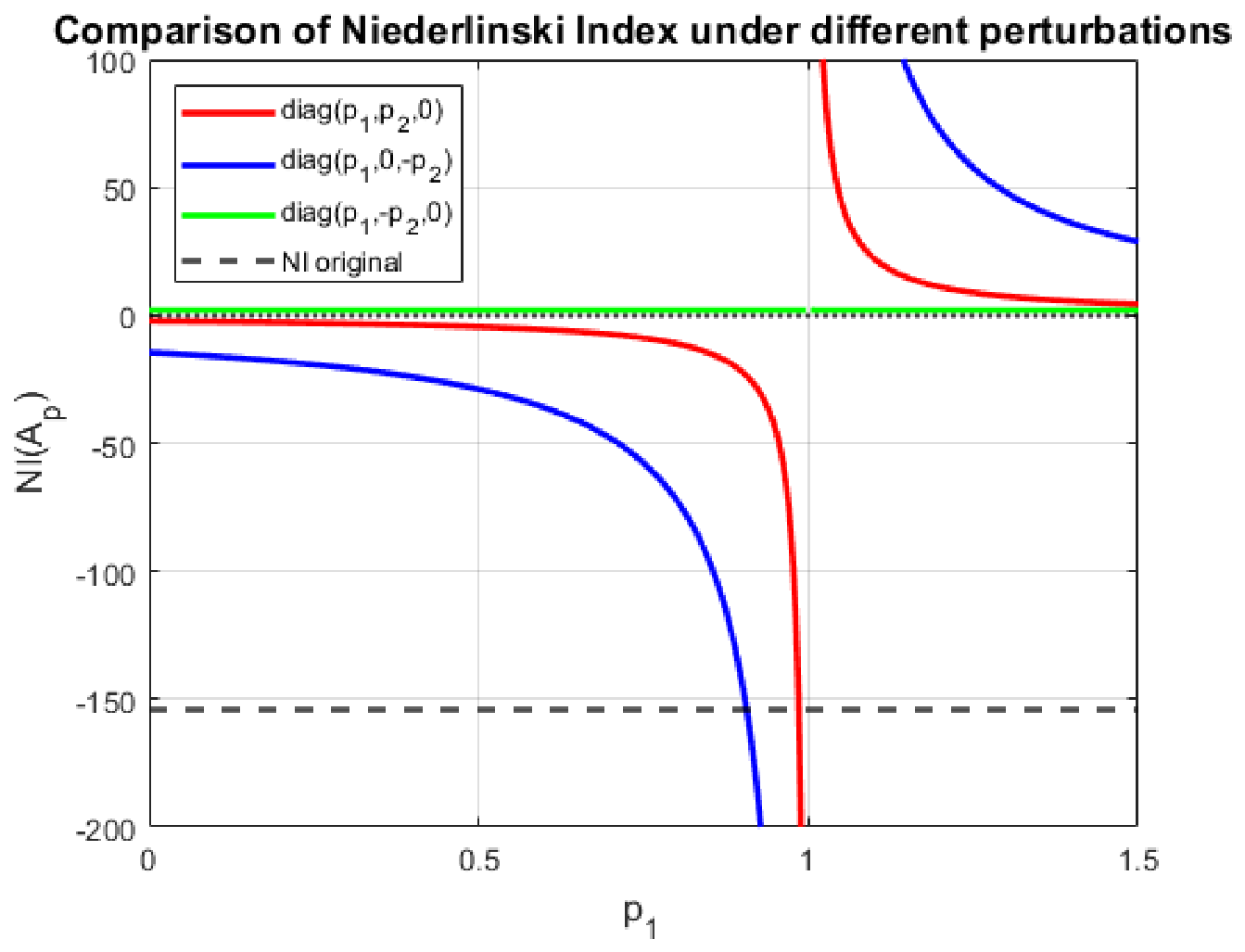
The previous examples demonstrate that stabilization can be achieved through different diagonal perturbation patterns. To provide a unified view, Figure 1 shows the evolution of the Niederlinski index $NI\left[A_p\right]$ as a function of $p_1$ for the three perturbation strategies considered.

The horizontal dashed line represents the original value $NI\left[A\right]<0$, corresponding to an unstable configuration. All three perturbation patterns produce a transition from negative to positive values, confirming that stabilization can be achieved in each case.

A clear difference in the behavior of the curves can be observed. First, the perturbations of the form $A+\mathrm{diag}(p_1,p_2,0)$ and $A+\mathrm{diag}(p_1,-p_2,0)$ exhibit a smooth transition, with stabilization occurring within a relatively narrow range of $p_1$. This indicates that modifying the $(2,2)$ entry provides an efficient mechanism to change the sign of the Niederlinski index.

In contrast, the perturbation $A+\mathrm{diag}(p_1,0,-p_2)$ shows a significantly different behavior. Although stabilization is still achieved, it requires much larger values of $p_2$, and the resulting index grows more abruptly. This reflects a lower sensitivity with respect to $p_1$ and highlights the stronger influence of the $(3,3)$ entry in this configuration.

Overall, the comparison reveals that, while all admissible perturbations are theoretically valid, their practical effectiveness differs substantially. In particular, perturbations involving the second diagonal entry are more efficient, whereas those involving the third diagonal entry require larger parameter variations.

For visualization purposes, the vertical axis in Figure 1 has been restricted in order to emphasize the transition region around the stability boundary $NI=0$.

5. Discussion

The numerical results presented in Section 4 provide a clear validation of the theoretical work developed in Section 3. In particular, the examples illustrate that diagonal perturbations allow one to systematically modify the sign of the Niederlinski index while preserving the doubly stochastic structure of the combined matrix.

From a structural point of view, the results indicate that stabilization is not achieved arbitrarily, but only within specific regions of the parameter space $(p_1,p_2)$. The pointwise examples confirm that the analytical bounds derived in Theorem 4 and Propositions 3–9 correctly identify admissible perturbations, while the global visualization reveals that these bounds capture a nontrivial subset of the stabilization region.

A key observation is that the proposed perturbations do not merely restore stability, but also produce a progressive improvement of the Niederlinski index. This behavior, clearly observed in the graphical representation, provides additional insight into the effectiveness of the method beyond binary stability criteria.

From an engineering perspective, these results admit a natural interpretation. Diagonal perturbations correspond to local modifications of subsystem dynamics, such as controller retuning, actuator calibration, or adjustment of loop gains. Therefore, the proposed paper provides explicit conditions under which such local actions lead to improved interaction properties while preserving the original coupling structure of the plant. This interpretation is consistent with classical approaches to decentralized control structure selection, where interaction measures and structural indices play a crucial role in assessing system performance and integrity [5].

The proposed methodology is formulated in terms of the Niederlinski index, which is a classical tool for assessing the feasibility of decentralized control configurations. Nevertheless, the Niederlinski index should not be regarded as a complete stability criterion. In particular, although a negative Niederlinski index is widely recognized as an indication that decentralized stabilization is generally impossible under the standard assumptions, a positive Niederlinski index alone does not guarantee closed-loop stability [1,3].

Furthermore, the Niederlinski index is derived from steady-state gain information and therefore does not capture dynamic effects such as pole–zero interactions, time delays, or higher-order dynamics. The stability of the closed-loop system also depends on the dynamic characteristics of the plant, the controller design, robustness margins, model uncertainty, and performance requirements.

Consequently, the results presented in this paper should be interpreted as providing algebraic conditions that eliminate a structural obstacle to decentralized stabilization, rather than as a complete stability analysis of the closed-loop system.

The method also highlights certain limitations. The analysis assumes that the interaction structure, as captured by the combined matrix, remains fixed under the perturbations. In practical applications, however, MIMO systems may be affected by uncertainties, external disturbances, or even adversarial interference, which can modify the effective system matrix and alter the interaction structure.

This issue is particularly relevant in communication and radar systems, where active interference may introduce additional inputs or significantly distort the nominal coupling structure. In such contexts, recent advances in interference detection and classification, such as the framework proposed by [10], provide complementary tools for identifying and mitigating these effects before they impact system performance [10].

Therefore, the stabilization conditions derived in this paper should be interpreted as nominal-model results, and their integration with data-driven identification or robust control techniques constitutes an interesting direction for future research.

Finally, although the present work focuses on third-order systems, the underlying concepts of combined matrices, diagonal equivalence, and structure-preserving perturbations extend naturally to higher-dimensional systems. The main difficulty lies in the increasing algebraic complexity of the associated conditions. The results presented here can therefore be seen as a first step towards a general theory of stabilization under structure-preserving constraints in MIMO systems.

6. Conclusions

In this paper, we have investigated the stabilization of third-order MIMO systems whose interaction structure is described by a doubly stochastic combined matrix. Starting from unstable configurations characterized by a negative Niederlinski index, we have derived explicit algebraic conditions under which stability can be recovered through diagonal perturbations while preserving the underlying interaction structure.

The proposed approach is based on a structured representation of the system matrix and on a detailed analysis of the perturbation polynomial governing the sign of the determinant. This allowed us to obtain explicit bounds on the perturbation parameters for different sign configurations, providing a complete characterization of admissible structure-preserving stabilization strategies.

The numerical results presented in Section 4 illustrate and validate the theoretical findings. In particular, the examples show that stabilization can be achieved for different perturbation patterns and sign regimes, while the global analysis highlights that the admissible parameter regions are nontrivial and consistent with the derived analytical bounds. Moreover, the results demonstrate that diagonal perturbations not only restore stability, but also produce a significant improvement in the value of the Niederlinski index.

From an engineering perspective, the proposed perturbations admit a natural interpretation in terms of local controller retuning and parameter adjustments, offering a constructive method for improving interaction properties without modifying the physical coupling structure of the system.

It should be emphasized that the Niederlinski index is used here as a structural indicator rather than as a complete stability criterion. Therefore, the results should be interpreted as identifying favorable regions for decentralized stabilization, which may be complemented by additional control-theoretic tools addressing robustness and dynamic performance.

From a computational viewpoint, the proposed approach is particularly efficient for third-order systems, since all stabilization conditions are derived analytically in closed form. Once the combined matrix has been computed, the admissible perturbation parameters are obtained by evaluating a finite set of explicit algebraic inequalities, without requiring iterative optimization procedures, eigenvalue computations, or numerical optimization algorithms. Therefore, the computational cost for the three-dimensional case is negligible.

For higher-order MIMO systems, the same methodology remains conceptually applicable. However, the number of interaction parameters, admissible perturbation cases, and algebraic inequalities increases rapidly with the system dimension. Consequently, although the proposed framework remains constructive, its computational complexity is expected to grow significantly, making symbolic manipulation and computer algebra techniques increasingly valuable for deriving explicit stabilization conditions.

Future research will focus on extending the proposed methodology to higher-dimensional systems, as well as on incorporating robustness considerations in the presence of uncertainties, disturbances, or external interference that may alter the interaction structure. The integration of structure-preserving stabilization with data-driven identification and advanced control techniques constitutes a promising direction for further investigation.

In this context, although the present work focuses on third-order MIMO systems, the underlying methodology relies on structural properties of combined matrices, diagonal equivalence, and the invariance of the Niederlinski index, which are not specific to dimension three. Therefore, the proposed approach provides a conceptual framework that can be extended to higher-order systems.

However, obtaining necessary and sufficient conditions in dimensions greater than three is expected to require substantially more involved algebraic characterizations and a significantly larger parameter space. Consequently, the extension of the present results to general $n\times n$ MIMO systems constitutes a natural and relevant direction for future research.