Hysteresis and Optimal Pricing of Subscriptions with Cancellation Cost

Abstract

We develop a stochastic Stackelberg model of a subscription market with cancellation costs. A representative consumer chooses when to subscribe to and cancel a service as the utility derived from the subscription evolves according to a diffusion process, while the firm selects the subscription fee and cancellation cost to maximize its expected payoff. The consumer’s problem is equivalent to the classical real-options model of entry and exit under uncertainty with adjustment costs and exhibits a two-threshold policy with an inaction band and hysteresis. Unlike the standard formulation, in which the optimal thresholds are characterized implicitly through a system of nonlinear equations, we derive an explicit parametric solution in closed form. This solution reduces the firm’s optimization problem to a two-dimensional unconstrained problem and yields a detailed characterization of the optimal pricing policy. We show that the firm’s strategy exhibits three qualitatively distinct regimes depending on the initial utility level. For small utility levels, the optimal cancellation cost is zero. In an intermediate regime, the firm’s optimal policy induces the consumer to set the entry threshold equal to the initial utility level, resulting in immediate subscription. For sufficiently large utility levels, the firm induces permanent lock-in by setting a high cancellation cost and a low subscription fee: the consumer subscribes immediately and never subsequently unsubscribes. The transition between the latter two regimes is discontinuous and results from competition between two local maxima of the firm’s payoff function. We then extend the model to a heterogeneous population of consumers. The superposition of individual two-threshold subscription strategies generates a Preisach hysteresis operator describing the aggregate dependence of the firm’s revenue on the utility dynamics. The discontinuous regime transition persists under heterogeneity, demonstrating the robustness of the underlying mechanism. The Preisach representation predicts complex history dependence and long-term effects of temporary utility shocks. For a gamma distribution of consumer preferences, the firm’s expected payoff is obtained in closed form in terms of incomplete gamma functions.

1. Introduction

The subscription economy has expanded rapidly in recent years. As of 2023, U.S. households spent on average USD 230 per month on subscription services [1], including mobile phone, internet, television streaming, Amazon Prime, and music streaming services. Reflecting the growing economic importance of subscription-based business models, a substantial literature has emerged on subscription pricing, consumer behavior, retention, and firm profitability [2,3]. Empirical studies indicate that subscription services can generate significant welfare effects for consumers [4] and that firms may profit from consumer adjustment costs, including switching costs and inattention, which contribute to inertia in subscription and cancellation decisions [5]. Such costs may be monetary, such as enrollment or cancellation fees, or nonmonetary, arising from search costs, effort, inconvenience, habit formation, and other behavioral frictions. For example, personalized recommendations have been shown to increase perceived switching costs by enhancing customer satisfaction and reinforcing habits [6].

A salient feature of many subscription services is the asymmetry between enrollment and cancellation: while subscribing is typically frictionless, cancellation often involves non-negligible costs or effort [7]. Motivated by this feature, we develop a stochastic optimal control model for analyzing subscription markets with cancellation costs.

We begin with a homogeneous market consisting of a single service provider (the firm) and a representative consumer. We then extend the model to a heterogeneous population of consumers with non-identical preferences. The interaction between the firm and consumers is modeled as a Stackelberg game. On the demand side, the consumer decides whether to subscribe to or cancel the service as the flow utility evolves over time. The utility process $X_t$, representing the value derived from the subscription, is modeled by a diffusion process. The other state variable is the binary state of a consumer (enrolled/unsubscribed) who takes as given the firm’s pricing structure, consisting of a subscription fee p and a cancellation cost $\xi$, and maximizes the expected discounted payoff (the follower’s problem). On the supply side, the firm anticipates the consumer’s optimal response and chooses $(p,\xi )$ to maximize its expected payoff (the leader’s problem).

More specifically, the consumer’s optimization problem coincides with the classical real-options model of entry and exit under uncertainty with adjustment costs studied in [8,9,10]. Accordingly, the utility process $X_t$ is modeled as a geometric Brownian motion, subscription and cancellation decisions correspond to entry and exit decisions, and the associated Hamilton–Jacobi–Bellman (HJB) variational inequality admits a two-threshold solution with an inaction band. There are thresholds $X_S$ and $X_U$ with $X_U<X_S$, such that the consumer subscribes when the flow utility $X_t$ exceeds $X_S$ and cancels when $X_t$ falls below $X_U$. The interval $(X_U,X_S)$ constitutes an inaction band: as long as $X_t$ remains within this region, the consumer does not change their state. Consequently, the consumer’s state exhibits hysteresis [8,11,12]; namely, it depends not only on the current value of $X_t$ but also on its past evolution. More broadly, hysteresis refers to history-dependent behavior in which the current state is determined by a sequence of past input values rather than by their timing [13].

In the classical real-options formulation, the optimal entry and exit thresholds $X_{S,U}$ are characterized by value-matching and smooth-pasting conditions and are typically obtained numerically from the resulting system of nonlinear equations [8,9,14]. In this work, we develop an explicit parametric representation of the solution. Specifically, we derive closed-form expressions

$$X_{S,U}=p{x}_{S,U}\left(\theta \right),\xi =p\epsilon \left(\theta \right),$$

(1)

where $x_{S,U}\left(\theta \right)$ and $\epsilon \left(\theta \right)$ are explicit functions of an auxiliary parameter $\theta$, which effectively replaces the adjustment-cost parameter $\xi$. Thus, the introduction of $\theta$ transforms the implicit nonlinear system of [8,9] into an explicit parametric solution (it is easily seen that $X_{S,U}$ are proportional to p). Then, we analyze the firm’s problem (the leader’s problem). Using the explicit expressions in (1) allows us to reduce the constrained optimization with four variables $X_S$, $X_U$, $p,\xi$ and two nonlinear constraints to the unconstrained optimization over $(p,\theta )$ yielding simple insights into the optimal solution. The firm’s optimal policy exhibits qualitatively different regimes depending on the initial state x. For small values of x, the firm optimally sets $\widehat{\xi }=0$, corresponding to costless cancellation, and the optimal subscription fee $\widehat{p}$ is constant over a range of x, yielding a single-threshold hysteresis-free consumer strategy with $X_S=X_U=\widehat{p}$. For large x, the optimal controls $(\widehat{p},\widehat{\xi })$ scale proportionally with x, and the firm’s optimal policy ensures that $X_U=0$, i.e., the consumer never cancels. Effectively, the high cancellation cost creates a permanent lock-in effect [15,16], keeping the consumer in the subscribed state. In the intermediate regime, the optimal controls depend on x in a more complicated manner. However, we show that in this case the optimal solution satisfies $X_S=x$, which leads to the closed-form expression $\widehat{p}=x/x_S\left(\widehat{\theta }\right)$ reducing the further analysis to one-dimensional optimization over $\theta$. Notably, it is shown that the dependence of $(\widehat{p},\widehat{\xi })$ on x exhibits a discontinuity at the border between the intermediate regime and the regime of large values of x, reflecting the fact that the firm’s payoff function has two competing local maxima, and the global optimum switches discontinuously from one to the other as x varies.

Finally, we incorporate consumer heterogeneity by allowing consumers to derive different levels of utility from the same service. Since each consumer follows a two-threshold subscription strategy, the aggregate mapping from utility dynamics to the firm’s revenue is obtained through the superposition of two-threshold nonlinearities and is described by the Preisach hysteresis operator, a classical hysteresis operator widely used in applications such as plasticity, friction, porous media, and magnetism [17]. As in the homogeneous setting, the explicit parametric representation of the consumer’s problem reduces the firm’s optimization problem to unconstrained optimization over $(p,\theta )$. The discontinuous transition between payoff-maximizing regimes persists under heterogeneity, demonstrating the robustness of the underlying mechanism.

Related formulations have appeared in the context of subscription markets with heterogeneous discounting under restrictive assumptions, such as small cancellation costs compared to the total cost of subscription [18]. In contrast, the framework of this work does not impose such constraints. More specifically, in [18], the firm’s payoff includes a large penalty term proportional to the cancellation cost; as such, the optimal cancellation cost is a priori small. This constraint, although not universal, can result from government interventions such as, for example, the final “click-to cancel” rule announced by the Federal Trade Commission in October 2024 that required sellers to make it as easy for consumers to cancel their enrollment as it was to sign up [7]. As it was shown in [18] in the case of a homogeneous market with one representative agent, the costless cancellation regime is optimal for the firm within a range $x\le x^{*}$ of smaller initial states, while for $x>x^{*}$ the optimal cancellation cost is positive and grows continuously with x. The point $x=x^{*}$ of the continuous transitions between these two regimes was computed explicitly. Moreover, asymptotic expressions for the consumer’s thresholds $X_{S,U}$ and the firm’s optimal controls $(\widehat{p},\widehat{\xi })$ were obtained for $x>x^{*}$ using the ratio $\epsilon$ of the cancellation cost to the total subscription cost as a small parameter. This asymptotic solution was then extended to the heterogeneous market with two representative consumers characterized by different discount rates.

In this paper, the firm’s payoff naturally increases with the subscription flow cost p and the number of subscriptions but does not depend directly on the subscription cancellation cost $\xi$; in particular, there is no penalty associated with $\xi$ as in [18]. However, the firm uses $\xi$ as an additional control as both p and $\xi$ affect the number of subscriptions through the consumer’s optimal strategy. In the case of a homogeneous market, the exact solution of the firm’s problem is naturally the same as in [18] in the range $x\le x^{*}$ where the cancellation cost is zero and is consistent with the asymptotic approximation obtained in [18] in a (limited) range of values $x>x^{*}$ for which the cancellation cost is sufficiently small. In addition, for all $x>x^{*}$, the firm’s optimal strategy induces the consumer to respond to the control $(\widehat{p},\widehat{\xi })$ by setting $X_S=x$, thus subscribing at the initial instant. This result is obtained using the closed-form solution $X_{S,U}=p{x}_{S,U}\left(\theta \right)$ of the consumer’s problem and seems intuitive. Moreover, the firm’s control strategies involving a relatively high cancellation cost, which are a priori ineffective in the setting of [18] as incurring a high penalty on the firm, can be effective in the penalty-free formulation adopted here. Indeed, as mentioned above, we show that if x is sufficiently large, $x>x_b$, then the firm’s optimal strategy leads the consumer to set $X_S=x$ and $X_U=0$. In other words, the consumer has a sufficient incentive to subscribe at the initial instant because the flow cost of subscription is sufficiently low, and never chooses to unsubscribe because the cancellation cost is too high. At the regime switching point at $x=x_b$, the firm abruptly increases the cancellation rate $\widehat{\xi }$ simultaneously decreasing the subscription flow rate $\widehat{p}$.

The closed-form solution of the consumer’s problem is used similarly in the heterogeneous setting. It should be noted that in the present setting the market heterogeneity is due to the consumers deriving different utility from the product, while in [18] it is due to a distribution of discount rates. The market with two representative consumers considered in [18] can be viewed as an extreme case of a bi-modal distribution of consumers. Here, we focus on a continuous uni-modal distribution. As such, some consumers subscribe at the initial instant, while the others wait until the utility grows higher. On the other hand, there are fractions of the population in different regimes: some unsubscribe when utility drops sufficiently low while others never unsubscribe once subscribed. Therefore, the firm maximizing its aggregate payoff does not enjoy the maximal flow benefit from any individual subgroup of consumers of positive measure. As a case study, we consider the gamma distribution of the utility coefficient. In this case, the firm’s expected payoff admits a closed-form expression in terms of incomplete gamma functions. Moreover, the firm’s flow revenue demonstrates complex history dependence, and so does the firm’s expected payoff. This form of history dependence, characteristic of the Preisach operator and arising from the superposition of two-threshold nonlinearities, is well understood [19]. The state at a time $\tau >0$ is determined by a sequence of selected local extremum values achieved by $X_t$ prior to $\tau$ (the so-called sequence of main extrema). If for example the global maximum value of $X_t$ over the time interval $[0,\tau ]$ precedes the global minimum value of $X_t$ over this interval, then the sequence of main extrema includes the global maximum value, followed by the global minimum value, then the largest maximum value achieved after the global minimum, followed by the smallest minimum value achieved thereafter and so on. As $X_t$ varies, so does the sequence of main extrema of $X_t$, which defines the composition of the subscribed and unsubscribed groups and, through this, the firm’s flow revenue from subscriptions.

The paper is organized as follows. In the next section, we formulate the model and derive the associated stochastic control problems for the consumer and the firm. The consumer’s problem is characterized via a variational inequality associated with the HJB equation, leading to the two-threshold solution. In Section 3, we present the solution of the consumer’s problem, first in the absence of cancellation costs and then for $\xi >0$. In Section 4, we analyze the firm’s optimization problem in the homogeneous market, including benchmark cases and a more general setting. In Section 5, we study a case of the firm’s problem under consumer heterogeneity and derive the corresponding hysteresis representation. Section 6 concludes.

2. Model

2.1. Dynamics

We let $(\mathsf{\Omega },\mathcal{F},\mathbb{P})$ denote a complete probability space that supports a standard Brownian motion ${\left(W_t\right)}_{t\ge 0}$ with its natural filtration ${\left({\mathcal{F}}_t\right)}_{t\ge 0}$. We denote the state variable by X and suppose that its dynamics are given by the diffusion process

$$d{X}_t=\mu X_{t}dt+\sigma X_{t}d{W}_t,X_0=x>0,$$

(2)

with the drift rate $\mu >0$ and the volatility parameter $\sigma >0$. We interpret $X_t$ as the flow certainty equivalent utility obtained by the consumer if currently subscribed to the service.

The second state variable is $Z\in \{0,1\}$, where 1 means the consumer is currently subscribed to the service and 0 means the consumer is currently not subscribed to (unsubscribed from) the service. There are costs from transitioning across these states. We denote by $\xi \ge 0$ the cancellation cost (i.e., of transitioning from 1 to 0). This cost can be the monetary cost of effort from taking the action, but also some monetary penalty paid by the consumer to the firm. We abstract away from this distinction for now. We also refrain from considering a positive or negative cost of enrolling to the service, which can be considered similarly [18].

Using an increasing sequence of times

$$\mathsf{\Xi }=(t_1,t_2,\dots ),0=t_0\le t_1<t_2<\dots ,$$

we denote by $Z_t:{\mathbb{R}}_{+}\to \{0,1\}$ the corresponding enrollment/cancellation policy

$$Z_t=\left\{\begin{array}{cc}z,\hfill & t_{2n}\le t<t_{2n+1},\hfill \\ 1-z,\hfill & t_{2n+1}\le t<t_{2n+2},\hfill \end{array}\right.n=0,1,2,\dots ,$$

(3)

where

$$Z_0=z\in \{0,1\}$$

(4)

is the initial state, i.e., $\mathsf{\Xi }$ is the sequence of transitioning times for $Z_t$. We denote by ${\mathsf{\Xi }}_S$ the set of times at which the consumer transitions from 0 to 1, respectively, ${\mathsf{\Xi }}_U$ are the times when the consumer transitions from 1 to 0. Hence, ${\mathsf{\Xi }}_S$ is the odd-indexed subsequence and ${\mathsf{\Xi }}_U$ is the even-indexed subsequence of $\mathsf{\Xi }$ if $z=0$; conversely, ${\mathsf{\Xi }}_S$ is the even-indexed subsequence and ${\mathsf{\Xi }}_U$ is the odd-indexed subsequence of $\mathsf{\Xi }$ if $z=1$.

We denote by $p>0$ the flow cost of the subscription. The expected payoff for an exponential discounter with discount rate r from a enrollment/cancellation policy $Z_t:{\mathbb{R}}_{+}\to \{0,1\}$ is given by

$$J(Z_t;x,z;p,\xi )=\mathbb{E}\left[{\int }_0^{\infty }{e}^{-rt}\left(X_t-p\right)Z_{t}dt-\xi \sum _{t\in {\mathsf{\Xi }}_U}{e}^{-rt}\right].$$

(5)

The consumer’s objective is to maximize the expected payoff using an admissible enrollment/cancellation policy as a control. Hence, the value function of this optimization problem is

$$V(x,z;p,\xi )=\underset{Z_t\in \mathcal{Z}}{sup}J(Z_t;x,z;p,\xi ),$$

where $\mathcal{Z}$ is the set of enrollment/cancellation policies $Z_t$ induced by transitioning time sequences $\mathsf{\Xi }$.

Since $X_t$ is a stationary Markov process, one expects optimal transitioning times to have the form of recursive stopping times

$$t_{n+1}=inf\{t\ge t_n:X_t\in {\mathcal{S}}_z\mathrm{with}z=Z_{t_n}\},n=0,1,2,\dots ,$$

(6)

where the closed set ${\mathcal{S}}_z\subset {\mathbb{R}}_{+}$ and its complement ${\mathcal{C}}_z={\mathbb{R}}_{+}\setminus {\mathcal{S}}_z$ are the so-called stopping and continuation regions, respectively, associated with the state $z\in \{0,1\}$ [20]. In other words, the consumer transitions from state z to state $1-z$ at the nearest moment when the process $X_t$ reaches the stopping region ${\mathcal{S}}_z$. In the simplest case, ${\mathcal{S}}_z$ is an interval with its end point(s) serving as threshold(s), i.e., a transition occurs when $X_t$ attains a threshold.

2.2. Variational Inequality and Two-Threshold Solution

For brevity, we occasionally write $V(x,z)=V(x,z;p,\xi )$ omitting the dependence on the parameters $p,\xi$. In order to solve for the optimal strategy and payoff, we represent the value function $V(x,z):{\mathbb{R}}_{+}\times \{0,1\}\to \mathbb{R}$ of a consumer as a pair of value functions

$$V_U\left(x\right)=V(x,0),V_S\left(x\right)=V(x,1)$$

corresponding to the states 0 and 1, respectively. The differential operator

$$\mathcal{L}V\left(x\right)=rV\left(x\right)-\mu x{V}^{\prime }\left(x\right)-{\displaystyle \frac{{\sigma }^2}{2}}{x}^2{V}^{\prime \prime }\left(x\right)$$

(7)

is associated in the usual way with the process (2) and the exponential discount rate r. As such, the value functions $V_S,V_C\in C^1\left({\mathbb{R}}_{+}\right)$ satisfy the following coupled variational inequalities (which are a form of the Bellman equation; see, e.g., refs. [20,21]):

$$\begin{array}{ccc}\hfill \mathcal{L}{V}_S\left(x\right)& \ge x-p,\hfill & \hfill a.e.x\in {\mathbb{R}}_{+},\end{array}$$

(8)

$$\begin{array}{ccc}\hfill V_S\left(x\right)& \ge V_U\left(x\right)-\xi ,\hfill & \hfill x\in {\mathbb{R}}_{+},\end{array}$$

(9)

$$\begin{array}{ccc}\hfill \left(\mathcal{L}{V}_S\left(x\right)-x+p\right)\left(V_S\left(x\right)-V_U\left(x\right)+\xi \right)& =0,\hfill & \hfill a.e.x\in {\mathbb{R}}_{+},\end{array}$$

(10)

and

$$\begin{array}{ccc}\hfill \mathcal{L}{V}_U\left(x\right)& \ge 0,\hfill & \hfill a.e.x\in {\mathbb{R}}_{+},\end{array}$$

(11)

$$\begin{array}{ccc}\hfill V_U\left(x\right)& \ge V_S\left(x\right),\hfill & \hfill x\in {\mathbb{R}}_{+},\end{array}$$

(12)

$$\begin{array}{ccc}\hfill \mathcal{L}{V}_U\left(x\right)\left(V_U\left(x\right)-V_S\left(x\right)\right)& =0,\hfill & \hfill a.e.x\in {\mathbb{R}}_{+}.\end{array}$$

(13)

In accordance with [22,23], the solution of this optimal control problem is naturally expected to involve two thresholds $X_U<X_S$ at which the consumer unsubcribes if their flow benefit falls below $X_U$ (when currently subscribed) and subscribes if their flow benefit reaches $X_S$ (when currently unsubscribed). In other words, the stopping and continuation regions for the state $z=1$ are

$${\mathcal{S}}_1=[0,X_U],{\mathcal{C}}_1=(X_U,\infty ),$$

(14)

and for the state $z=0$ they are

$${\mathcal{S}}_0=[X_S,\infty ),{\mathcal{C}}_0=(0,X_S).$$

(15)

For this solution in the continuation region, the HJB variational inequality (8)–(13) leads to the equations

$$\begin{array}{ccc}\hfill \mathcal{L}{V}_S\left(x\right)& =x-p,\hfill & \hfill x>X_U,\end{array}$$

(16)

$$\begin{array}{ccc}\hfill \mathcal{L}{V}_U\left(x\right)& =0,\hfill & \hfill x<X_S,\end{array}$$

(17)

coupled to the value matching conditions

$$V_S\left(X_S\right)-V_U\left(X_S\right)=0,V_S\left(X_U\right)-V_U\left(X_U\right)=-\xi ,$$

(18)

the smooth pasting conditions

$${\displaystyle \frac{d}{dX}}\left(V_S\left(X_S\right)-V_U\left(X_S\right)\right)={\displaystyle \frac{d}{dX}}\left(V_S\left(X_U\right)-V_U\left(X_U\right)\right)=0$$

(19)

at the thresholds $X_S$, $X_U$, and the conditions

$$V_U\left(0\right)=0,\underset{x\to \infty }{lim\; sup}{\displaystyle \frac{V_S\left(x\right)}{x}}<\infty$$

(20)

at zero and infinity. On the other hand, in the stopping region the HJB variational inequality yields

$$\begin{array}{ccc}\hfill V_S\left(x\right)& =V_U\left(x\right)-\xi ,\hfill & \hfill x\le X_U,\end{array}$$

(21)

$$\begin{array}{ccc}\hfill V_U\left(x\right)& =V_S\left(x\right),\hfill & \hfill x\ge X_S.\end{array}$$

(22)

The corresponding transitioning policy is the sequence of stopping times (6) defined by the threshold-based rule

$$t_{n+1}=\left\{\begin{array}{ccc}inf\{t\ge t_n:X_t\ge X_S\}\hfill & \mathrm{if}& Z_{t_n}=0,\hfill \\ inf\{t\ge t_n:X_t\le X_U\}\hfill & \mathrm{if}& Z_{t_n}=1,\hfill \end{array}\right.n=0,1,2,\dots ,$$

(23)

i.e., a transition across the states occurs when $X_t$ hits either the threshold $X_S$ or $X_U$ (depending on the current state) as well as at the initial moment if the initial conditions satisfy either $x=X_0\ge X_S$ and $z=Z_0=0$ or $x=X_0\le X_U$ and $z=Z_0=1$.

Remark 1.

The variational inequality (8)–(13) requires that

$$\begin{array}{ccc}\hfill \mathcal{L}{V}_S\left(x\right)& \ge x-p,\hfill & \hfill x<X_U,\end{array}$$

(24)

$$\begin{array}{ccc}\hfill V_S\left(x\right)& \ge V_U\left(x\right)-\xi ,\hfill & \hfill x>X_U,\end{array}$$

(25)

$$\begin{array}{ccc}\hfill \mathcal{L}{V}_U\left(x\right)& \ge 0,\hfill & \hfill x>X_S,\end{array}$$

(26)

$$\begin{array}{ccc}\hfill V_U\left(x\right)& \ge V_S\left(x\right),\hfill & \hfill x<X_S.\end{array}$$

(27)

As shown in [18], if $V_S:[X_U,\infty )\to \mathbb{R}$, $V_U:[0,X_S]\to \mathbb{R}$ is a solution of Problem (16)–(20) extended to ${\mathbb{R}}_{+}\ni x$ by Equations (21) and (22), then Relations (24)–(27) hold iff

$$\begin{array}{cc}\hfill X_U& -p+r\xi \le 0,\hfill \end{array}$$

(28)

$$\begin{array}{cc}\hfill X_S& -p\ge 0.\hfill \end{array}$$

(29)

We denote by $\delta ,\gamma$ with $\gamma <0<\delta$ the roots of the characteristic polynomial

$$L\left(m\right):=-{\displaystyle \frac{1}{2}}{\sigma }^{2}m(m-1)-\mu m+r$$

(30)

associated with the differential operator $\mathcal{L}$. In what follows, it is assumed that characteristic polynomial (30) satisfies

$$L\left(1\right)=r-\mu >0,$$

(31)

which is equivalent to

$$L\left(\gamma \right)=L\left(\delta \right)=0,\gamma <0,\delta >1.$$

(32)

Remark 2.

Applying boundary Conditions (18)–(20) to the general solution of Euler’s Equations (16) and (17) results in

$$V_S\left(x\right)={\displaystyle \frac{x}{r-\mu }}-{\displaystyle \frac{p}{r}}+B_S{x}^{\gamma },x>X_U;V_U\left(x\right)=A_U{x}^{\delta },x<X_S,$$

(33)

with

$$B_S={\displaystyle \frac{(1-\delta )X_S^{-\gamma }}{(r-\mu )(\delta -\gamma )}}\left(X_S+\left({\displaystyle \frac{1}{\gamma }}-1\right)p\right),A_U={\displaystyle \frac{(1-\gamma )X_S^{-\delta }}{(r-\mu )(\delta -\gamma )}}\left(X_S+\left({\displaystyle \frac{1}{\delta }}-1\right)p\right)$$

(34)

and the system

$$X_S^{1-\gamma }+\left({\displaystyle \frac{1}{\gamma }}-1\right)p{X}_S^{-\gamma }=X_U^{1-\gamma }+\left({\displaystyle \frac{1}{\gamma }}-1\right)(p-r\xi )X_U^{-\gamma },$$

(35)

$$X_S^{1-\delta }+\left({\displaystyle \frac{1}{\delta }}-1\right)p{X}_S^{-\delta }=X_U^{1-\delta }+\left({\displaystyle \frac{1}{\delta }}-1\right)(p-r\xi )X_U^{-\delta }$$

(36)

for the thresholds $X_{S,U}$. As shown in [18], Relations (32) warrant the solvability of System (35) and (36) in the domain (28) and (29), thus providing a two-threshold solution for the HJB variational inequality (8)–(13) in accordance with Remark 1.

Remark 3.

The payoff

$$J_{\alpha }(Z_t;x,z;p,\xi )=\mathbb{E}\left[{\int }_0^{\infty }{e}^{-rt}\left(X_t^{\alpha }-p\right)Z_{t}dt-\xi \sum _{t\in {\mathsf{\Xi }}_U}{e}^{-rt}\right]$$

with any $\alpha >0$ is equivalent to (5). Indeed, (2) implies that ${\tilde{X}}_t=X_t^{\alpha }$ is a geometric Brownian motion with modified percentage drift and volatility, i.e.,

$${\tilde{X}}_t=\tilde{\mu }{\tilde{X}}_{t}dt+\tilde{\sigma }{\tilde{X}}_{t}d{W}_t\mathrm{with}\tilde{\mu }=\alpha \left(\mu +{\displaystyle \frac{\alpha -1}{2}}{\sigma }^2\right),\tilde{\sigma }=\alpha \sigma .$$

The characteristic polynomial of the associated differential operator has roots $\gamma /\alpha$ and $\delta /\alpha$.

2.3. Heterogeneous Consumer Market and Firm Problem

Now, we consider a heterogeneous market in which consumers derive different utility from the product. More precisely, given a Borel set $\mathsf{\Omega }\subset {\mathbb{R}}_{+}$, we associate a parameter $\rho \in \mathsf{\Omega }$ with each consumer and assume that they derive the flow utility $\rho X_t$ when currently subscribed to the service, where the state $X_t$ evolves according to (2). As such, each consumer maximizes their expected payoff

$$\mathbb{E}\left[{\int }_0^{\infty }{e}^{-rt}\left(\rho X_t-p\right)Z_t\left(\rho \right)dt-\xi \sum _{t\in {\mathsf{\Xi }}_U}{e}^{-rt}\right]=\rho J\left(Z_t\left(\rho \right);x,z_{\rho };p/\rho ,\xi /\rho \right)$$

(37)

(cf. (5)), where $Z_t\left(\rho \right)$ denotes the enrollment/cancellation policy of the consumer and $z_{\rho }=Z_0\left(\rho \right)$ denotes their initial state. Accordingly, the state of the market at time t is the pair $(X_t,Z_t(·))$, where the second component is a Borel function $Z_t\left(\rho \right):\mathsf{\Omega }\to \{0,1\}$.

Next, we extend the model by introducing the service providing firm, thus closing the feedback loop. To this end, a cumulative distribution function $F\left(\rho \right):\mathsf{\Omega }\to [0,1]$ is associated with the distribution of the parameter $\rho$ over the set $\mathsf{\Omega }$, i.e., over the consumer population. We assume that the flow benefit of the firm from each subscription is $p-c$. Hence, the aggregated flow benefit from all the subscriptions at time t equals

$$Y_t=(p-c){\int }_{\mathsf{\Omega }}{Z}_t\left(\rho \right)dF\left(\rho \right),$$

(38)

and the expected payoff of the firm in the case $\mathsf{\Omega }={\mathbb{R}}_{+}$ is

$$\widehat{J}(Z_t(·);x,z(·),p;\xi )=\mathbb{E}\left[{\int }_0^{\infty }{\int }_0^{\infty }{e}^{-rt}(p-c)Z_t\left(\rho \right)dtdF\left(\rho \right)\right],$$

(39)

where $(x,z(·))=(X_0,Z_0(·))$ is the initial state of the market.

The firm sets the flow rate p and the cancellation cost $\xi$ seeking to maximize its expected payoff (39), while each consumer sets their enrollment/cancellation thresholds $X_{S,U}(\rho ;p,\xi )$ based on the values of p, $\xi$ seeking to maximize payoff (37). The thresholds $X_{S,U}(\rho ;p,\xi )$ determine the enrollment/cancellation policy $Z_t\left(\rho \right)$, which feeds back to (39).

Remark 4.

The homogeneous market of identical consumers corresponds to $F=H_1$ with the Heaviside step function

$$H_1\left(x\right)=\left\{\begin{array}{cc}0,\hfill & \hfill x<1,\\ 1,\hfill & \hfill x>1.\end{array}\right.$$

(40)

2.4. Relation to Preisach Model

Relations (3), (4) and (6) define a map from any space of continuous inputs $X_t:{\mathbb{R}}_{+}\to {\mathbb{R}}_{+}$ (not necessarily realizations of the Geometric Brownian Motion) to the space of binary functions $Z_t:{\mathbb{R}}_{+}\to \{0,1\}$. In the case when the stopping and continuation regions have the form (14) and (15) with $X_U<X_S$, i.e., (6) has the form (23), this map is well-known in engineering applications as the two-threshold two-state non-ideal relay (also known as bi-stable switch, “lazy” switch, elementary rectangular hysteresis loop, or Schmitt trigger depending on a particular application).

Stacking a set non-ideal relays, which all have the same input $X_t:{\mathbb{R}}_{+}\to \mathbb{R}$ but different thresholds, and defining the output $Y_t:{\mathbb{R}}_{+}\to \mathbb{R}$ of the system as the aggregated quantity (38), have a long history in applied physics and engineering, starting from the fundamental phenomenological model of magnetic hysteresis developed by F. Preisach [24]. The composition of the mapping of inputs to state trajectories $(X_t,Z_t(·))$ and the state-output functional (38) is called the Preisach operator [13,19,25]. Its equivalent counterparts and special cases used in other disciplines include the Prandtl–Ishlinskii model in plasticity [26], Maxwell-slip friction model in tribology [27,28] and Parlange model in hydrology [29] with further applications to control based on smart materials [30,31,32,33,34], neuroscience [35], epidemiology [36,37], economics [11,38,39,40] and real options [18].

Remark 5.

Throughout this paper, the parameter ρ in (38) is scalar. In most engineering applications, ρ is two-dimensional. A more general market model can include a population of consumers with different payoffs $X^{\alpha }-p$ (cf. Remark 3) and different discount rates $r>0$, leading to the Preisach operator with the parameter $\rho =(\alpha ,r)$ distributed over a two-dimensional domain Ω in the firm’s payoff. The market where the consumers differ by the discount rate only was considered in [18].

2.5. Model Assumptions

The model is designed to capture the interaction of consumer heterogeneity, switching costs, and hysteresis in subscription markets while remaining analytically tractable. To this end, several simplifying assumptions are adopted.

First, consumer utility is represented by a geometric Brownian motion. This choice follows the standard real-options framework and yields a tractable characterization of optimal subscription and cancellation decisions.

Second, the subscription fee and cancellation cost are assumed to be fixed upon contract design and do not depend on subsequent realizations of the utility process. The firm’s problem is therefore formulated as an optimization over contract parameters rather than a dynamic pricing problem.

Third, consumer heterogeneity is represented by a single parameter measuring the utility derived from the service. Although the analysis is carried out for a one-dimensional distribution of consumer types, the associated Preisach representation extends naturally to bivariate and higher-dimensional parameter distributions. Additional sources of heterogeneity may include risk preferences, switching-cost sensitivities, or discount rates (see [18]).

Finally, the market is assumed to consist of a representative firm. Consumers therefore choose only between subscribing and not subscribing, without the possibility of switching to a competing provider.

These assumptions isolate the effects of consumer heterogeneity and switching costs on subscription dynamics and allow the resulting hysteretic behavior to be characterized explicitly. We discuss several important avenues for extension in the concluding section.

3. Consumer Problem

3.1. Costless Cancellation Benchmark

We start with the consumer problem. As a benchmark case, let us consider zero cancellation cost, i.e., $\xi =0$. In this case, Relations (21), (22), (25) and (27) imply $V_S\left(x\right)=V_U\left(x\right)$ on the whole ${\mathbb{R}}_{+}$, hence we simply write $V:=V_S=V_U$. Moreover, from (16) and (17) it follows that $X_S=X_U$ and

$$\begin{array}{ccc}\hfill \mathcal{L}V\left(x\right)& =x-p,\hfill & \hfill x>X_{*},\end{array}$$

(41)

$$\begin{array}{ccc}\hfill \mathcal{L}V\left(x\right)& =0,\hfill & \hfill x<X_{*},\end{array}$$

(42)

where $X_{*}:=X_S=X_U$. Combining these equations with (24) and (26) results in

$$\begin{array}{ccc}\hfill x-p& \le \mathcal{L}V\left(x\right)=0,\hfill & \hfill x<X_{*},\\ \hfill 0& \le \mathcal{L}V\left(x\right)=x-p,\hfill & \hfill x>X_{*},\end{array}$$

therefore

$$X_{*}=p.$$

(43)

Using solutions (33) of Equations (41) and (42) and applying the value matching and smooth pasting conditions at the threshold (43), one obtains the $C^2\left({\mathbb{R}}_{+}\right)$ value function

$$V\left(x\right)=p·\left\{\begin{array}{cc}{\displaystyle A{\left(\frac{x}{p}\right)}^{\delta },}\hfill & \hfill x\le p,\\ {\displaystyle \frac{1}{L\left(1\right)}\left(\frac{x}{p}\right)-\frac{1}{r}+B{\left(\frac{x}{p}\right)}^{\gamma },}\hfill & \hfill x>p,\end{array}\right.$$

with

$$A={\displaystyle \frac{r(1-\gamma )+\gamma L\left(1\right)}{r(\delta -\gamma )L\left(1\right)}},B={\displaystyle \frac{r(1-\delta )+\delta L\left(1\right)}{r(\delta -\gamma )L\left(1\right)}}.$$

The corresponding transitioning policy is the single-threshold rule

$$Z_t=H_{X_{*}}\left(X_t\right),$$

(44)

where $H_{X_{*}}$ is the Heaviside step function

$$H_{X_{*}}\left(x\right)=\left\{\begin{array}{cc}0,\hfill & \hfill x<X_{*},\\ 1,\hfill & \hfill x>X_{*}.\end{array}\right.$$

(45)

Accordingly, the consumer is subscribed whenever $X_t>X_{*}$, unsubscribed whenever $X_t<X_{*}$, and transitions from state 0 to 1 and vice versa at the same threshold $X_t=X_{*}=p.$

3.2. Non-Zero Cancellation Cost

Next, let us consider a non-zero cancellation cost $\xi >0$ and the corresponding optimal two-threshold strategy of the consumer. According to Remark 2, the optimal thresholds can be obtained from Systems (35) and (36) and should satisfy (28) and (29). We introduce the variable

$$\theta ={\displaystyle \frac{X_S}{X_U}}>1$$

(46)

and replace the cancellation cost $\xi$ with the dimensionless parameter

$$\epsilon ={\displaystyle \frac{{\sigma }^2\xi }{2p}}.$$

(47)

Proposition 1.

For every

$$0<\epsilon <-{\displaystyle \frac{1}{\delta \gamma }}={\displaystyle \frac{{\sigma }^2}{2r}},$$

System (35) and (36) has a unique solution. This solution satisfies Relations (28) and (29) and can be written in the parametric form

$$X_S=p{x}_S\left(\theta \right),X_U={\theta }^{-1}{X}_S,x_S\left(\theta \right):={\displaystyle \frac{(1-\delta )(1-\gamma )\left({\theta }^{1-\delta }-{\theta }^{1-\gamma }\right)}{\gamma (1-\delta ){\theta }^{1-\gamma }-\delta (1-\gamma ){\theta }^{1-\delta }+\delta -\gamma }},$$

(48)

$$\epsilon \left(\theta \right)=-{\displaystyle \frac{1}{\delta \gamma }}\left(1-{\theta }^{-\gamma }-{\displaystyle \frac{\gamma x_S\left(\theta \right)}{1-\gamma }}({\theta }^{-\gamma }-{\theta }^{-1})\right)$$

(49)

with $\theta >1$. Moreover, $X_{S,U}=X_{S,U}\left(\theta \right)$, $x_S=x_S\left(\theta \right)$ and $\epsilon =\epsilon \left(\theta \right)$ satisfy

$$X_{S,U}\to p,x_S\to 1,\epsilon \to 0\mathrm{as}\theta \to 1+$$

(50)

and

$${\displaystyle \frac{d{X}_S}{d\theta }}>0>{\displaystyle \frac{d{X}_U}{d\theta }},{\displaystyle \frac{d\epsilon }{d\theta }}>0\mathrm{for}\mathrm{all}\theta >1.$$

(51)

We extend the functions $x_S\left(\theta \right),\epsilon \left(\theta \right)$ from the open interval $\theta >1$ by continuity to the closed interval $\theta \ge 1$ as

$$x_S\left(1\right)=1,\epsilon \left(1\right)=0.$$

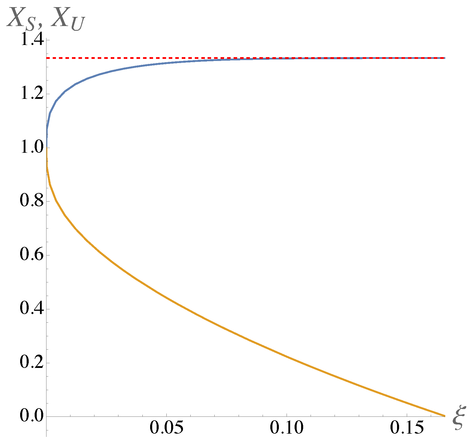
Figure 1 shows the dependence of the thresholds $X_{S,U}$ on the cancellation cost $\xi$.

Remark 6.

Proposition 1 implies the asymptotic formulas

$${\displaystyle \frac{X_S}{p}}=1+{\displaystyle \frac{\theta -1}{2}}+{\displaystyle \frac{\delta +\gamma -2}{12}}{(\theta -1)}^2+{\displaystyle \frac{\delta \gamma -\delta -\gamma +2}{24}}{(\theta -1)}^3+O\left({(\theta -1)}^4\right),$$

(52)

$${\displaystyle \frac{X_U}{p}}=1-{\displaystyle \frac{\theta -1}{2}}+{\displaystyle \frac{\delta +\gamma +4}{12}}{(\theta -1)}^2+{\displaystyle \frac{\delta \gamma -3\delta -3\gamma -6}{24}}{(\theta -1)}^3+O\left({(\theta -1)}^4\right),$$

(53)

$$\epsilon ={\displaystyle \frac{{(\theta -1)}^3}{12}}+O\left({(\theta -1)}^4\right),$$

(54)

where $\theta \to 1$. These formulas agree with the asymptotic expansions

$${\displaystyle \frac{X_S}{p}}=1+{\displaystyle \sum _{n=1}^N}{a}_n^S{\epsilon }^{n/3}+O({\epsilon }^{{\displaystyle \frac{N+1}{3}}}),{\displaystyle \frac{X_U}{p}}=1+{\displaystyle \sum _{n=1}^N}{a}_n^U{\epsilon }^{n/3}+O({\epsilon }^{{\displaystyle \frac{N+1}{3}}}),\epsilon \to 0,$$

(55)

obtained in [18]. As an example, for $N=5$, denoting

$$\lambda =1-{\displaystyle \frac{2\mu }{{\sigma }^2}}=\delta +\gamma ,\tau =-{\displaystyle \frac{2r}{{\sigma }^2}}=\delta \gamma ,$$

(56)

the coefficients in (55) are

$$\begin{array}{cc}\hfill a_1^S& =-a_1^U=\sqrt[3]{{\displaystyle \frac{3}{2}}},\hfill \end{array}$$

(57)

$$\begin{array}{cc}\hfill a_2^S& =a_2^U={\displaystyle \frac{1+\lambda }{\sqrt[3]{12}}},\hfill \end{array}$$

(58)

$$\begin{array}{cc}\hfill a_3^S& ={\displaystyle \frac{1}{30}}\left(1+11\lambda +{\lambda }^2+9\tau \right),\hfill \end{array}$$

(59)

$$\begin{array}{cc}\hfill a_3^U& =-a_3^S+\tau ,\hfill \end{array}$$

(60)

$$\begin{array}{cc}\hfill a_4^S& ={\displaystyle \frac{1}{30\sqrt[3]{18}}}\left(-1+6\lambda +6{\lambda }^2-{\lambda }^3+3\left(7+3\lambda \right)\tau \right),\hfill \end{array}$$

(61)

$$\begin{array}{cc}\hfill a_4^U& =a_4^S-{\displaystyle \frac{2\tau }{\sqrt[3]{18}}},\hfill \end{array}$$

(62)

$$\begin{array}{cc}\hfill a_5^S& ={\displaystyle \frac{1}{3150\sqrt[3]{12}}}\left(-2-44\lambda \right.+159{\lambda }^2-44{\lambda }^3-2{\lambda }^4+3(178+328\lambda \left.\left.-12{\lambda }^2\right)\tau -243{\tau }^2\right),\hfill \end{array}$$

(63)

$$\begin{array}{cc}\hfill a_5^U& =-a_5^S+{\displaystyle \frac{(1+\lambda )\tau }{3\sqrt[3]{12}}}.\hfill \end{array}$$

(64)

Remark 7.

Equations (48) and (49) imply that

$$X_S\to {\displaystyle \frac{p(\gamma -1)}{\gamma }},X_U\to 0,x_S\left(\theta \right)\to 1-{\displaystyle \frac{1}{\gamma }},\epsilon \to -{\displaystyle \frac{1}{\delta \gamma }}={\displaystyle \frac{{\sigma }^2}{2r}}\mathrm{as}\theta \to \infty .$$

(65)

This limit corresponds to the no-cancellation policy. Namely, for any $\epsilon \ge -1/\left(\delta \gamma \right)$, the consumer never unsubscribes once they subscribe (the state “subscribed” becomes absorbing). Moreover, the optimal subscription threshold is $X_S=p(\gamma -1)/\gamma$, i.e., if $x\ge p(\gamma -1)/\gamma$, then the consumer subscribes at the initial instant; if $x<p(\gamma -1)/\gamma$, then the consumer subscribes at the first instant when $X_t$ reaches the threshold $X_S=p(\gamma -1)/\gamma$. For this limit, we use the notation

$$\theta =\infty ;x_S(\infty )=\underset{\theta \to \infty }{lim}{x}_S\left(\theta \right)=1-{\displaystyle \frac{1}{\gamma }}.$$

(66)

Thus,

• $\theta =1$ induces the single-threshold switching policy of the consumer with the enrollment/cancellation threshold $X_{S,U}=p$;
• $0<\theta <\infty$ induces the two-threshold switching policy of the consumer with the enrollment threshold $X_S=p{x}_S\left(\theta \right)$ and cancellation threshold $X_U={\theta }^{-1}{X}_S$;
• $\theta =\infty$ induces the no-cancellation policy of the consumer (once subscribed, the consumer never unsubscribes) with the enrollment threshold $X_S=p(\gamma -1)/\gamma$.

Proof of Proposition 1.

Combining (35) and (36) and using the variable (46) and the parameter (47), one obtains the equations

$$\left({\displaystyle \frac{1}{\delta }}-1\right)\left(X_U\left({\theta }^{1-\gamma }-1\right)+\left({\displaystyle \frac{1}{\gamma }}-1\right)p{\theta }^{-\gamma }\right)=\left({\displaystyle \frac{1}{\gamma }}-1\right)\left(X_U\left({\theta }^{1-\delta }-1\right)+\left({\displaystyle \frac{1}{\delta }}-1\right)p{\theta }^{-\delta }\right),$$

$$\left({\displaystyle \frac{1}{\gamma }}-1\right)(1+\delta \gamma \epsilon )p=X_U\left({\theta }^{1-\gamma }-1\right)+\left({\displaystyle \frac{1}{\gamma }}-1\right)p{\theta }^{-\gamma },$$

which imply (48) and (49). Moreover, the Taylor expansions (52)–(54) of (48) and (49) imply (50). By inspection,

$${\displaystyle \frac{d{X}_S}{d\theta }}={\displaystyle \frac{(1-\delta )(1-\gamma )(\gamma -\delta ){\theta }^{\delta +\gamma +1}\left((1-\gamma ){\theta }^{\delta -1}-(1-\delta ){\theta }^{\gamma -1}+\gamma -\delta \right)}{{\left((\gamma -\delta ){\theta }^{\delta +\gamma }-\gamma {\theta }^{1+\delta }+\delta {\theta }^{1+\gamma }+\delta \gamma ({\theta }^{1+\delta }-{\theta }^{1+\gamma })\right)}^2}},$$

(67)

$${\displaystyle \frac{d{X}_U}{d\theta }}={\displaystyle \frac{(1-\delta )(1-\gamma )\left(\delta {\theta }^{\gamma }-\gamma {\theta }^{\delta }\right){\theta }^{\delta +\gamma -1}\left((1-\gamma ){\theta }^{1-\delta }-(1-\delta ){\theta }^{1-\gamma }+\gamma -\delta \right)}{{\left((\gamma -\delta ){\theta }^{\delta +\gamma }-\gamma {\theta }^{1+\delta }+\delta {\theta }^{1+\gamma }+\delta \gamma ({\theta }^{1+\delta }-{\theta }^{1+\gamma })\right)}^2}},$$

(68)

$${\displaystyle \frac{d\epsilon }{d\theta }}={\displaystyle \frac{{\theta }^{\delta +\gamma }\left((1-\gamma ){\theta }^{\delta -1}-(1-\delta ){\theta }^{\gamma -1}+\gamma -\delta \right)\left((1-\gamma ){\theta }^{1-\delta }-(1-\delta ){\theta }^{1-\gamma }+\gamma -\delta \right)}{{\left((\gamma -\delta ){\theta }^{\delta +\gamma }-\gamma {\theta }^{1+\delta }+\delta {\theta }^{1+\gamma }+\delta \gamma ({\theta }^{1+\delta }-{\theta }^{1+\gamma })\right)}^2}}.$$

(69)

Since $(a^u-1)/u$ is a strictly increasing function of u for any positive $a\ne 1$, the relations $\gamma <0<1<\delta$ imply

$${\displaystyle \frac{{\theta }^{\delta -1}-1}{1-\delta }}<{\displaystyle \frac{{\theta }^{\gamma -1}-1}{1-\gamma }};{\displaystyle \frac{{\theta }^{1-\delta }-1}{1-\delta }}<{\displaystyle \frac{{\theta }^{1-\gamma }-1}{1-\gamma }};{\displaystyle \frac{\gamma }{1-{\theta }^{-\gamma }}}<{\displaystyle \frac{\delta }{1-{\theta }^{-\delta }}}.$$

(70)

Combining these relations with (67) and (68) gives (51). □

4. Firm Problem: Homogeneous Consumer Market

4.1. Costless Cancellation Benchmark

In this section, we consider the firm problem stated in Section 2.3 in the homogeneous market (i.e., one representative consumer, see Remark 4). We start again with the costless cancellation benchmark, i.e., the firm is committed to the zero cancellation cost $\xi =0$. As such, the firm uses a single parameter p (the flow payoff) to maximize its expected payoff. In the case of one consumer with the transitioning policy (44) (see Section 3.1), the expected firm’s payoff (39) equals

$$W^0(x;p):=\mathbb{E}\left[{\int }_0^{\infty }{e}^{-rt}(p-c)H_{X_{*}}\left(X_t\right)dt\right].$$

Therefore, the payoff $W^0(·;p)\in C^1\left({\mathbb{R}}_{+}\right)$ can be obtained as a solution of the differential equation

$$\mathcal{L}{W}^0(x;p)=(p-c)H_{X_{*}}\left(x\right)$$

(71)

(cf. (7)) subject to the boundary conditions

$$W^0(0;p)=0,\underset{x\in {\mathbb{R}}_{+}}{sup}{W}^0(x;p)<\infty .$$

(72)

Using the value matching and smooth pasting conditions at the discontinuity point (43) of the step function gives

$$W^0(x;p)={\displaystyle \frac{1}{r}}·\left\{\begin{array}{cc}{\displaystyle W_S^0(x;p):=(p-c)\left(1-\frac{\delta }{\delta -\gamma }{\left(\frac{x}{p}\right)}^{\gamma }\right),}\hfill & p<x,\hfill \\ {\displaystyle W_U^0(x;p):=-\frac{\gamma (p-c)}{\delta -\gamma }{\left(\frac{x}{p}\right)}^{\delta },}\hfill & p\ge x.\hfill \end{array}\right.$$

(73)

Proposition 2.

The payoff (73) of the firm achieves its unique maximum with respect to p at the point

$$p^{*}\left(x\right):=\underset{p>0}{arg\; max}{W}^0(x;·)=\left\{\begin{array}{cc}{\displaystyle x^{*},}\hfill & x\le x^{*},\hfill \\ p_S^{*}\left(x\right),\hfill & x>x^{*},\hfill \end{array}\right.$$

(74)

where

$$x^{*}={\displaystyle \frac{c\delta }{\delta -1}}$$

(75)

and $p_S^{*}\left(x\right)$ is a unique positive root p of the equation

$$\eta (x;p):=1-{\displaystyle \frac{\delta (1-\gamma )}{\delta -\gamma }}{\left({\displaystyle \frac{x}{p}}\right)}^{\gamma }-{\displaystyle \frac{c\delta \gamma }{(\delta -\gamma )p}}{\left({\displaystyle \frac{x}{p}}\right)}^{\gamma }=0.$$

(76)

Function (74) satisfies

$$p^{*}\left(x\right)>c\mathit{for}\mathit{all}x>0;$$

(77)

$$x^{*}<p_S^{*}\left(x\right)=p^{*}\left(x\right)<x\mathit{for}x>x^{*};p^{*}\left(x\right)=x^{*}>x\mathit{for}x<x^{*}.$$

(78)

Proof. 

By inspection, for a fixed x,

$$W_S^0(x;0)=-c;W_S^0(x;p)\to -\infty \mathrm{as}p\to \infty ;$$

$$W_U^0(x;p)\to -\infty \mathrm{as}p\to 0;W_U^0(x;p)\to 0\mathrm{as}p\to \infty ,$$

and each of the functions $W_{S,U}^0$ (as functions of $p>0$) has a unique maximum. Namely

$$\underset{p>0}{arg\; max}{W}_U^0(x;·)=x^{*}$$

does not depend on x; on the other hand,

$$p_S^{*}\left(x\right):=\underset{p>0}{arg\; max}{W}_S^0(x;·)$$

is a unique positive root p of Equation (76). Therefore, the payoff achieves its maximum with respect to p at the point (74). By inspection, $x>x^{*}$ is equivalent to $\eta (x;x)<0$, hence $x>x^{*}$ iff $x>p_S^{*}\left(x\right)$. Also, $x^{*}>c$, hence if $x>x^{*}$, then

$$\eta (x;c)=1-{\displaystyle \frac{\delta }{\delta -\gamma }}{\left({\displaystyle \frac{x}{c}}\right)}^{\gamma }>0,\eta (x;x^{*})=1-{\left({\displaystyle \frac{x}{x^{*}}}\right)}^{\gamma }>0$$

and consequently $c<x^{*}<p_S^{*}\left(x\right)$. Therefore, (77) holds and

$$c<x^{*}<p_S^{*}\left(x\right)<x\mathrm{if}x>x^{*},$$

which combined with $p^{*}\left(x\right)=x^{*}$ for $x<x^{*}$ implies (78). □

The firm maximizes its payoff by setting $p=p^{*}\left(x\right)$ depending on the initial value $X_0=x$ of the state variable. In particular, if the initial state satisfies

$$x<x^{*}={\displaystyle \frac{c\delta }{\delta -1}},$$

(79)

then the firm sets $p=x^{*}$, i.e., the firm’s expected payoff is

$$W^0(x;x^{*})=-{\displaystyle \frac{c\gamma }{r(\delta -1)(\delta -\gamma )}}{\left({\displaystyle \frac{x(\delta -1)}{c\delta }}\right)}^{\delta },x<{\displaystyle \frac{c\delta }{\delta -1}}.$$

(80)

Since $x<p=x^{*}$, the consumer is unsubscribed at the initial moment in accordance with transitioning policy (44). On the other hand, if

$$x>x^{*}={\displaystyle \frac{c\delta }{\delta -1}},$$

then the firm sets $p=p_S^{*}\left(x\right)$, and the expected payoff is

$$W^0(\chi ;p_S^{*}\left(x\right))={\displaystyle \frac{p_S^{*}\left({\chi }_0\right)-c}{r}}\left(1-{\displaystyle \frac{\delta }{\delta -\gamma }}{\left({\displaystyle \frac{x}{p_S^{*}\left(x\right)}}\right)}^{\gamma }\right),x>p_S^{*}\left(x\right).$$

(81)

Here, due to (78), from $x>x^{*}$ it follows that $x>p^{*}\left(x\right)$, hence the consumer is subscribed at the initial moment.

4.2. Non-Zero Cancellation Cost: Firm’s Value Function

Assume that the firm sets the flow payoff rate $p>0$ and the cancellation cost $\xi \ge 0$. In response, the consumer implements the two-threshold strategy, and the expected payoff of the firm satisfies the equations

$$\begin{array}{ccc}\hfill \mathcal{L}{W}_S\left(x\right)=& p-c,\hfill & \hfill x>X_U,\end{array}$$

(82)

$$\begin{array}{ccc}\hfill \mathcal{L}{W}_U\left(x\right)=& 0,\hfill & \hfill x<X_S,\end{array}$$

(83)

where the subscripts $S,U$ correspond to the state of the consumer. These equations are combined with the boundary conditions

$$W_U\left(0\right)=0,\underset{X\in {\mathbb{R}}_{+}}{sup}{W}_S\left(x\right)<\infty$$

(84)

at zero and infinity, resulting in the relations

$$\begin{array}{cc}\hfill W_S\left(x\right)=& {\displaystyle \frac{p-c}{r}}+{\widehat{B}}_S{x}^{\gamma },\hfill \end{array}$$

(85)

$$\begin{array}{cc}\hfill W_U\left(x\right)=& {\widehat{A}}_U{x}^{\delta }\hfill \end{array}$$

(86)

(cf. (71) and (72)), where the coefficients are determined by the value matching relations at the thresholds:

$${\displaystyle \frac{p-c}{r}}+{\widehat{B}}_S{X}_S^{\gamma }={\widehat{A}}_U{X}_S^{\delta },{\displaystyle \frac{p-c}{r}}+{\widehat{B}}_S{X}_U^{\gamma }={\widehat{A}}_U{X}_U^{\delta }.$$

(87)

Recall that the consumer sets the thresholds $X_{S,U}$ to maximize their payoff depending on the flow rate p and cancellation cost $\xi$, hence the coefficients ${\widehat{A}}_U,{\widehat{B}}_S$ and the firm’s payoff $W_{S,U}$ are functions of $p,\xi$ or, equivalently, of $p,\theta$; see Proposition 1. The payoff also depends on the initial state of the consumer.

To be specific, let us assume that the consumer is initially unsubscribed unless $x\ge X_S$. In this case, Equations (48), (85) and (86) imply that the firm’s payoff equals

$$W(x;p,\theta )=\left\{\begin{array}{cc}{\displaystyle W_S(x;p,\theta ):=\frac{p-c}{r}\left(1-\omega \left(\theta \right){\left(\frac{x}{p{x}_S\left(\theta \right)}\right)}^{\gamma }\right),}\hfill & p{x}_S\left(\theta \right)<x,\hfill \\ {\displaystyle W_U(x;p,\theta ):=\frac{p-c}{r}\left(1-\omega \left(\theta \right)\right){\left(\frac{x}{p{x}_S\left(\theta \right)}\right)}^{\delta },}\hfill & p{x}_S\left(\theta \right)\ge x,\hfill \end{array}\right.$$

(88)

where

$$\omega \left(\theta \right):={\displaystyle \frac{{\theta }^{\delta }-1}{{\theta }^{\delta -\gamma }-1}}.$$

(89)

As such, the firm’s value function $\widehat{W}$ is defined by

$$\widehat{W}\left(x\right)=\underset{p>0,\theta >1}{sup}W(x;p,\theta ),$$

(90)

and a pair $(\widehat{p},\widehat{\theta })$ is an optimal firm’s policy (optimal control) if

$$W(x;\widehat{p},\widehat{\theta })=\widehat{W}\left(x\right).$$

(91)

As expected, payoff (88) converges to payoff (73) in the costless cancellation case as $\theta \to 1$.

4.3. Auxiliary Statements

The following statement characterizes payoff (88) as a function of $\theta$ with fixed $x,p$ and on the curve $x=p{x}_S\left(\theta \right)$ with a fixed x where $W_U=W_S$.

Proposition 3.

For any $x>0$, $\theta \ge 1$, each of the functions $W_{S,U}(x;·,\theta )$ defined in (88) has a unique point $p=p_{S,U}^{*}(x;\theta )$ of global maximum on the interval $p\ge c$, i.e.,

$$W_{S,U}\left(x;p_{S,U}^{*}(x;\theta ),\theta \right)>W_{S,U}(x;p,\theta )\mathit{for}\mathit{all}x>0,\theta \ge 1,p\ge c,p\ne p_{S,U}^{*}(x;\theta ).$$

As such, $p_{S,U}^{*}$ is a continuous function of the variables $x>0,$ $\theta >1$ satisfying $p_{S,U}^{*}\ge c$. Moreover, for any $x>0,$ $\theta \ge 1$ either $p=p_{S,U}^{*}(x;\theta )$ is a unique critical point of the function $W_{S,U}(x;·,\theta )$ in the interval $p>c$, i.e.,

$${\displaystyle \frac{\partial W_{S,U}}{\partial p}}(x;p,\theta )>0,c\le p<p_{S,U}^{*}(x;\theta );{\displaystyle \frac{\partial W_{S,U}}{\partial p}}(x;p_{S,U}^{*}(x;\theta ),\theta )=0;{\displaystyle \frac{\partial W_{S,U}}{\partial p}}(x;p,\theta )<0,p>p_{S,U}^{*}(x;\theta ),$$

or

$$p_{S,U}^{*}(x;\theta )=c;W_{S,U}(x;p,\theta )<0,{\displaystyle \frac{\partial W_U}{\partial p}}(x;p,\theta )<0\mathit{for}\mathit{all}p>c.$$

Proof. 

By inspection,

$${\displaystyle \frac{{\partial }^2{W}_S}{\partial p^2}}(x;p,\theta )=\left(p(1-\gamma )+c(1+\gamma )\right){\displaystyle \frac{\gamma \left({\theta }^{\delta }-1\right)}{r{p}^2\left({\theta }^{\delta -\gamma }-1\right)}}{\left({\displaystyle \frac{x}{p{x}_S\left(\theta \right)}}\right)}^{\gamma },$$

$${\displaystyle \frac{{\partial }^2{W}_U}{\partial p^2}}(x;p,\theta )=\left(p(\delta -1)-c(\delta +1)\right){\displaystyle \frac{\delta \left(1-{\theta }^{\gamma }\right)}{r{p}^2\left(1-{\theta }^{\gamma -\delta }\right)}}{\left({\displaystyle \frac{x}{p{x}_S\left(\theta \right)}}\right)}^{\delta },$$

hence

$${\displaystyle \frac{{\partial }^2{W}_S}{\partial p^2}}(x;p,\theta )<0\mathrm{for}\mathrm{all}p\ge c;$$

(92)

$${\displaystyle \frac{{\partial }^2{W}_U}{\partial p^2}}(x;p,\theta )<0\mathrm{for}c\le p<{\displaystyle \frac{c(\delta +1)}{\delta -1}},{\displaystyle \frac{{\partial }^2{W}_U}{\partial p^2}}(x;p,\theta )>0\mathrm{for}p>{\displaystyle \frac{c(\delta +1)}{\delta -1}}.$$

(93)

On the other hand,

$$r{\displaystyle \frac{\partial W_S}{\partial p}}(x;p,\theta )=1-\left(1-\gamma +{\displaystyle \frac{c\gamma }{p}}\right){\displaystyle \frac{{\theta }^{\delta }-1}{{\theta }^{\delta -\gamma }-1}}{\left({\displaystyle \frac{x}{p{x}_S\left(\theta \right)}}\right)}^{\gamma },$$

(94)

$$r{\displaystyle \frac{\partial W_U}{\partial p}}(x;p,\theta )=\left(1-\delta +{\displaystyle \frac{c\delta }{p}}\right){\displaystyle \frac{1-{\theta }^{\gamma }}{1-{\theta }^{\gamma -\delta }}}{\left({\displaystyle \frac{x}{p{x}_S\left(\theta \right)}}\right)}^{\delta },$$

(95)

hence

$${\displaystyle \frac{\partial W_{S,U}}{\partial p}}(x;p,\theta )<0\mathrm{for}\mathrm{all}\mathrm{sufficiently}\mathrm{large}p.$$

(96)

All the conclusions of the proposition follow from (92)–(96) and $W_{S,U}(x;c,\theta )\le 0$. □

Remark 8.

A unique critical point of the function $W_U(x;·,\theta )$ in the interval $p>c$ is $p=x^{*}$ as in the costless cancellation case, i.e., $\theta =1$, cf. (75). A unique critical point of the function $W_S(x;·,\theta )$ in the interval $p>c$ is a unique positive root p of the equation

$$1+(1-\gamma )\varphi \left(\theta \right){\left({\displaystyle \frac{x}{p}}\right)}^{\gamma }+{\displaystyle \frac{c\gamma \varphi \left(\theta \right)}{p}}{\left({\displaystyle \frac{x}{p}}\right)}^{\gamma }=0,$$

where $\varphi \left(\theta \right)$ is defined below in (98) (cf. (76) for $\theta =1$).

Proposition 4.

The following relations hold:

$$W_S(x;p,\theta )={\displaystyle \frac{p-c}{r}}\left(1-{\displaystyle \frac{\delta }{\delta -\gamma }}{\left({\displaystyle \frac{x}{p}}\right)}^{\gamma }\left(1+{\displaystyle \frac{\gamma (1-3\gamma )}{24}}{(\theta -1)}^2\right)\right)+O\left({(\theta -1)}^3\right),\theta \to 1,$$

$$W_U(x;p,\theta )={\displaystyle \frac{\gamma (p-c)}{r(\gamma -\delta )}}{\left({\displaystyle \frac{x}{p}}\right)}^{\delta }\left(1+{\displaystyle \frac{\delta (1-3\delta )}{24}}{(\theta -1)}^2\right)+O\left({(\theta -1)}^3\right),\theta \to 1,$$

$$W_{S,U}(x;x/x_S\left(\theta \right),\theta )={\displaystyle \frac{\gamma }{r(\gamma -\delta )}}\left(x-c+{\displaystyle \frac{\delta -1}{2}}(x-x^{*})(\theta -1)\right)+O\left({(\theta -1)}^2\right),\theta \to 1,$$

$$W_S(x;p,\theta )={\displaystyle \frac{p-c}{r}}\left(1-{\left({\displaystyle \frac{x\gamma }{p(\gamma -1)}}\right)}^{\gamma }\left({\theta }^{\gamma }+o\left({\theta }^{\gamma }\right)\right)\right),\theta \to \infty ,$$

$$W_U(x;p,\theta )={\displaystyle \frac{p-c}{r}}{\left({\displaystyle \frac{x\gamma }{p(\gamma -1)}}\right)}^{\delta }\left(1-{\theta }^{\gamma }+o\left({\theta }^{\gamma }\right)\right),\theta \to \infty ,$$

$$W_{S,U}(x;x/x_S\left(\theta \right),\theta )={\displaystyle \frac{1}{r}}\left({\displaystyle \frac{x\gamma }{\gamma -1}}-c\right)\left(1-{\theta }^{\gamma }+o\left({\theta }^{\gamma }\right)\right),\theta \to \infty ,$$

$${\displaystyle \frac{d}{d\theta }}\left(W_{S,U}(x;x/x_S\left(\theta \right),\theta )\right)=-{\displaystyle \frac{\gamma }{r}}\left({\displaystyle \frac{x\gamma }{\gamma -1}}-c\right)\left({\theta }^{\gamma -1}+o\left({\theta }^{\gamma -1}\right)\right),\theta \to \infty .$$

Proof. 

The statement follows directly from (48) and (88). □

Set

$$x^{**}:={\displaystyle \frac{x^{*}(\gamma -1)}{\gamma }}={\displaystyle \frac{c\delta (\gamma -1)}{(\delta -1)\gamma }},$$

(97)

and define the functions

$$\varphi \left(\theta \right)=-{\displaystyle \frac{{\theta }^{\delta }-1}{{\theta }^{\delta -\gamma }-1}}{x}_S{\left(\theta \right)}^{-\gamma },\psi \left(\theta \right)={\displaystyle \frac{{\theta }^{\delta -\gamma }-{\theta }^{\delta }}{{\theta }^{\delta -\gamma }-1}}{x}_S{\left(\theta \right)}^{-1},\phi \left(\theta \right)={\displaystyle \frac{{\theta }^{\delta -\gamma }-{\theta }^{\delta }}{{\theta }^{\delta -\gamma }-1}}{x}_S{\left(\theta \right)}^{-\delta }.$$

(98)

Equations (88) and (98) imply

$$W_S(x;p,\theta )={\displaystyle \frac{p-c}{r}}\left(1+\varphi \left(\theta \right){\left({\displaystyle \frac{x}{p}}\right)}^{\gamma }\right),W_U(x;p,\theta )={\displaystyle \frac{p-c}{r}}\phi \left(\theta \right){\left({\displaystyle \frac{x}{p}}\right)}^{\delta },$$

(99)

$$W_{S,U}\left(x;x/x_S\left(\theta \right),\theta \right)={\displaystyle \frac{x-c{x}_S\left(\theta \right)}{r}}\psi \left(\theta \right).$$

(100)

Remark 9.

Proposition 4 implies that:

• The function $W_S(x;p,·)$ (with fixed $x,p$) has a local minimum at the point $\theta =1$, converges to its limit at infinity from below, and

  $$W_S(x;p,1)<{\displaystyle \frac{p-c}{r}}=W_S(x;p,\infty )$$
  (we racall the notation $\theta =\infty$ for the limit $\theta \to \infty$ from (66)).
• The function $W_U(x;p,·)$ has a local maximum at the point $\theta =1$, converges to its limit at infinity from below, and

  $$W_U(x;p,1)={\displaystyle \frac{\gamma (p-c)}{r(\gamma -\delta )}}{\left({\displaystyle \frac{x}{p}}\right)}^{\delta }>{\displaystyle \frac{p-c}{r}}{\left({\displaystyle \frac{x\gamma }{p(\gamma -1)}}\right)}^{\delta }=W_U(x;p,\infty ).$$
• On the curve $p=x/x_S\left(\theta \right)$, the function $W=W_S=W_U$ satisfies

  $$(x-x^{*})\underset{\theta \to 1}{lim}{\displaystyle \frac{d}{d\theta }}\left(W_{S,U}(x;x/x_S\left(\theta \right),\theta )\right)>0,x\ne x^{*};$$

  (101)

  $$(x-x^{**})\left(W_{S,U}\left(x;x/x_S(\infty ),\infty \right)-W_{S,U}\left(x;x/x_S\left(1\right),1\right)\right)>0,x\ne x^{**},$$

  (102)

  and (since (97) implies $x^{**}>c(\gamma -1)/\gamma$) if $x\ge x^{**}$, the function $W_{S,U}(x;x/x_S(·),·)$ converges to its limit at infinity from below. As such, there is a $\mathsf{\Theta }>0$ such that every local maximum of the function $W_{S,U}(x;x/x_S(·),·)$ belongs to the interval $[0,\mathsf{\Theta }]$, i.e.,

  $$W_{S,U}\left(x;x/x_S\left(\widehat{\theta }\right),\widehat{\theta }\right)=\underset{\theta \ge 1}{sup}{W}_{S,U}\left(x;x/x_S\left(\theta \right),\theta \right),x>0,1\le \widehat{\theta }<\infty \Rightarrow \widehat{\theta }\le \mathsf{\Theta }.$$

  (103)
  Moreover, in the limit $x\to \infty$,

  $$\underset{x\to \infty }{lim}{\displaystyle \frac{r}{x}}{W}_{S,U}\left(x;x/x_S\left(\theta \right),\theta \right)=\psi \left(\theta \right),$$

  (104)

  where the function $\psi \left(\theta \right)$ defined in (98) converges to its limit at infinity from below and satisfies

  $${\displaystyle \frac{d\psi }{d\theta }}\left(1\right)={\displaystyle \frac{(\delta -1)\gamma }{2(\gamma -\delta )}}>0,\underset{\theta \to \infty }{lim}\psi \left(\theta \right)-\psi \left(1\right)={\displaystyle \frac{\gamma }{\gamma -1}}-{\displaystyle \frac{\gamma }{\gamma -\delta }}>0.$$

We complete this section with the following technical statement.

Proposition 5.

For any $x^{*}<x<x^{**}$ and θ defined by $x=x^{*}{x}_S\left(\theta \right)$,

$$W_{S,U}\left(x;x/x_S\left(1\right),1\right)>W_{S,U}\left(x;x/x_S\left(\theta \right),\theta \right),W_{S,U}\left(x;x/x_S\left(1\right),1\right)>W_U(x;x^{*},\infty ).$$

(105)

Proof. 

Set

$$g\left(\theta \right)={\displaystyle \frac{{\theta }^{\gamma }-1}{(\delta -1)({\theta }^{\delta }-{\theta }^{\gamma })}}+{\displaystyle \frac{\gamma ({\theta }^{\gamma }-\theta )}{\gamma {\theta }^{\delta }(\theta -{\theta }^{\gamma })+\delta \left((\gamma -1){\theta }^{1+\gamma }-\gamma {\theta }^{1+\delta }+{\theta }^{\gamma +\delta }\right)}}.$$

By inspection, $x=x^{*}{x}_S\left(\theta \right)$ and (48) imply

$$W_{S,U}\left(x;x/x_S\left(1\right),1\right)-W_{S,U}\left(x;x^{*},\theta \right)={\displaystyle \frac{c{\theta }^{\delta }}{r}}g\left(\theta \right).$$

Hence, the first relation in (105) is equivalent to $g\left(\theta \right)>0$. Using the positive parameters $\mathsf{\ell }=-\gamma$, $q=\delta -1$, the function g can be written equivalently as

$$g\left(\theta \right)={\displaystyle \frac{\mathsf{\ell }q({\theta }^{\mathsf{\ell }+q+1}-1)(\theta -1)-(\mathsf{\ell }+q+1)\theta ({\theta }^{\mathsf{\ell }}-1)({\theta }^q-1)}{q({\theta }^{\mathsf{\ell }+q+1}-1)\theta \left((\mathsf{\ell }+q+1)({\theta }^q-1)+\mathsf{\ell }q({\theta }^{\mathsf{\ell }+q+1}-1)\right)}},$$

hence $g\left(\theta \right)>0$ holds iff

$$\mathsf{\ell }q({\theta }^{\mathsf{\ell }+q+1}-1)(\theta -1)>(\mathsf{\ell }+q+1)\theta ({\theta }^{\mathsf{\ell }}-1)({\theta }^q-1).$$

(106)

Moreover, introducing the notation

$$\varkappa \left(u\right)=ln\left({\displaystyle \frac{{\theta }^u-1}{u{\theta }^{u/2}}}\right),$$

inequality (106) is equivalent to

$$\varkappa (\mathsf{\ell }+q+1)+\varkappa \left(1\right)>\varkappa (\mathsf{\ell })+\varkappa \left(q\right).$$

(107)

Now,

$${\displaystyle \frac{d^2\varkappa }{d{u}^2}}={\displaystyle \frac{{({\theta }^u-1)}^2-{\theta }^u{u}^2{ln}^2\theta }{u^2{({\theta }^u-1)}^2}}={\displaystyle \frac{\left({\theta }^u-1+{\theta }^{u/2}uln\theta \right)\left({\theta }^u-1-{\theta }^{u/2}uln\theta \right)}{u^2{({\theta }^u-1)}^2}},$$

hence from the relations

$${\theta }^u-1-{\theta }^{u/2}uln\theta ={\theta }^{u/2}\left({\theta }^{u/2}-{\theta }^{-u/2}-uln\theta \right)=2{\theta }^{u/2}\left(sinh\left({\displaystyle \frac{uln\theta }{2}}\right)-{\displaystyle \frac{uln\theta }{2}}\right)>0,$$

it follows that ${\displaystyle \frac{d^2\varkappa }{d{u}^2}}>0$, i.e., $\varkappa \left(u\right)$ is convex on $u\ge 0$. Moreover,

$$\varkappa \left(0\right)=ln(ln\theta ),{\displaystyle \frac{d\varkappa }{du}}\left(0\right)=0,$$

and therefore the function $\varkappa \left(u\right)$ increases on $u\ge 0$. Using the monotonicity and convexity of $\varkappa$,

$$\varkappa (\mathsf{\ell }+q+1)-\varkappa (\mathsf{\ell })>\varkappa (\mathsf{\ell }+q)-\varkappa (\mathsf{\ell })>\varkappa \left(q\right)-\varkappa \left(0\right)>\varkappa \left(q\right)-\varkappa \left(1\right),$$

which implies (107) and proves the first of relations (105).

On the other hand, by inspection,

$$W_{S,U}\left(x;x/x_S\left(1\right),1\right)-W_U(x;x^{*},\infty )={\displaystyle \frac{x^{**}}{r}}h\left(v\right),$$

where

$$h\left(v\right):={\displaystyle \frac{\gamma }{\gamma -\delta }}\left(v-{\displaystyle \frac{(\delta -1)\gamma }{\delta (\gamma -1)}}\right)-{\displaystyle \frac{\gamma }{\delta (\gamma -1)}}{v}^{\delta },v={\displaystyle \frac{x}{x^{**}}},$$

hence the second of Relations (105) is equivalent to

$$h\left(v\right)>0,\gamma /(\gamma -1)<v<1.$$

(108)

From $\delta >1$, it follows that h is a concave function. Moreover, $h\left(1\right)=0$ and

$$h\left({\displaystyle \frac{\gamma }{\gamma -1}}\right)={\displaystyle \frac{\gamma }{\delta (\gamma -1)}}\left({\displaystyle \frac{\gamma }{\gamma -\delta }}-{\left({\displaystyle \frac{\gamma }{\gamma -1}}\right)}^{\delta }\right).$$

(109)

Due to Bernoulli’s inequality,

$${\left({\displaystyle \frac{\gamma -1}{\gamma }}\right)}^{\delta }>{\displaystyle \frac{\gamma -\delta }{\gamma }},$$

hence (109) implies $h(\gamma /(\gamma -1\left)\right)>0$, which combined with $h\left(1\right)=0$ and the concavity of h implies (108), completing the proof. □

4.4. Zero Operating Cost Benchmark

Assume that the operating cost is negligible, i.e., $c=0$.

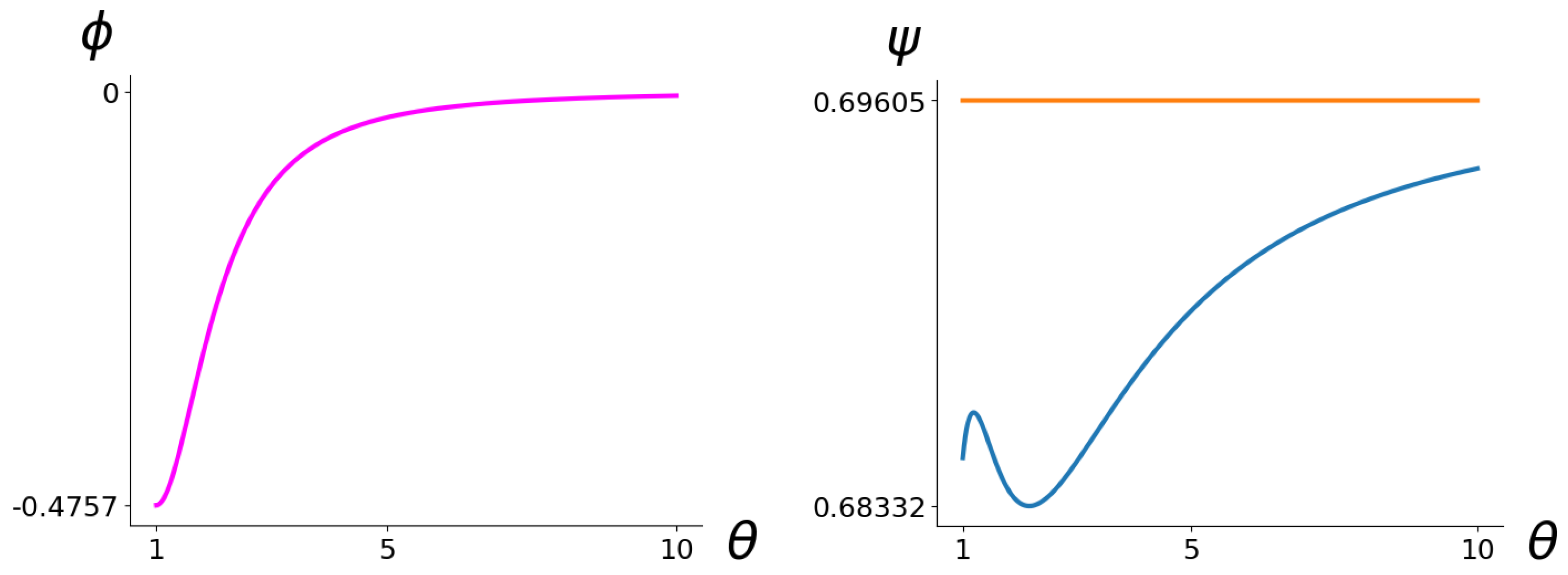
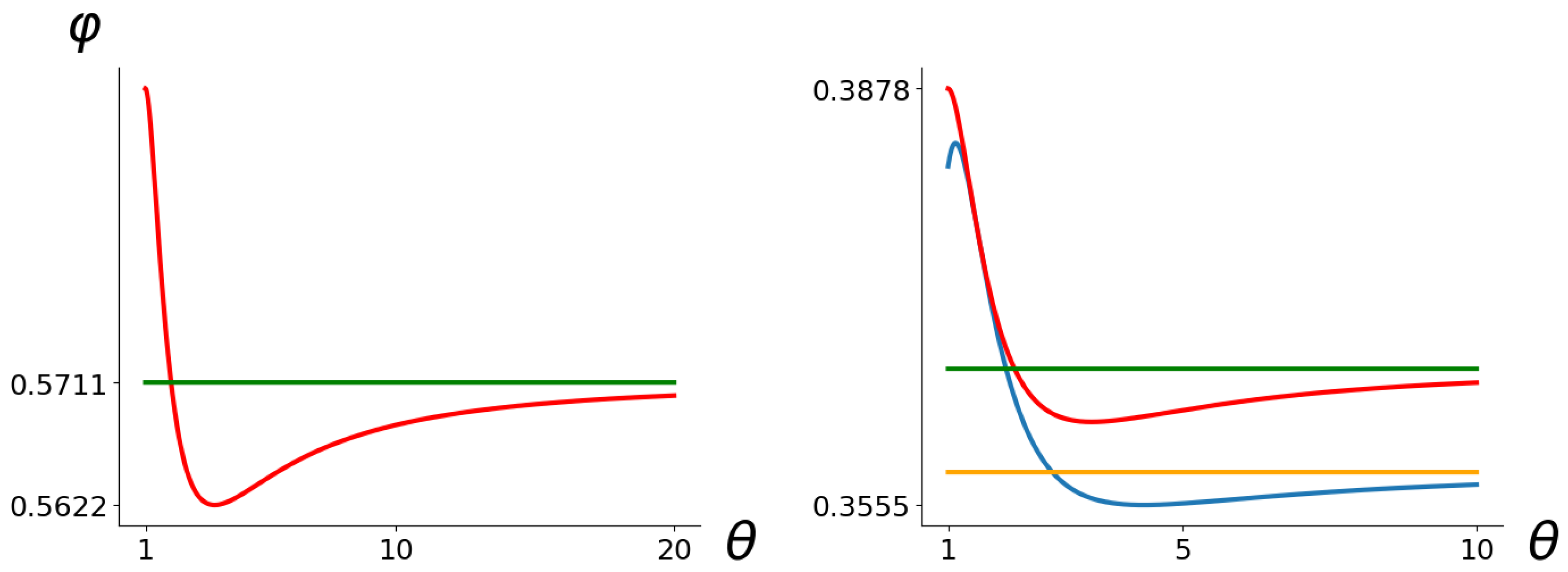
Figure 2 and Figure 3 (left panel) present typical graphs of Functions (98). We identify the following global features of these graphs:

(i)

Function $\varphi \left(\theta \right)$ increases.

(ii)

Function $\psi \left(\theta \right)$ satisfies $\psi \left(\theta \right)<\psi (\infty )$ for all $1\le \theta <\infty$.

(iii)

Function $\phi \left(\theta \right)$ satisfies $\phi \left(\theta \right)<\phi \left(1\right)$ for all $1<\theta \le \infty$ and has no local maxima for $\theta >1$.

Remark 10.

The global features (i)–(iii) agree with the asymptotic relations stated in Proposition 4 according to (99) and (100).

Proposition 6.

If $c=0$, then Relations (i)–(ii) imply that the optimal firm’s policy is $\widehat{p}=x\gamma /(\gamma -1)$ and $\widehat{\theta }=\infty$, i.e., $\xi =-\widehat{p}/\left(\delta \gamma \right)=x\gamma {\sigma }^2/\left(2r(\gamma -1)\right)$.

These optimal control parameters ensure that the enrollment threshold $X_S$ is placed at $X_S=X_0=x$, hence the consumer subscribes at the initial instant. Moreover, according to Remark 7, this control induces the no-cancellation policy of the consumer who never cancels the subscription due to the high cancellation cost.

Proof of Proposition 6.

If $x<p{x}_S\left(\theta \right)$, then $W=W_U$ decreases in p. As such, the maximum for a fixed $\theta$ is achieved at the point $x=p{x}_S\left(\theta \right)$.

If $x>p{x}_S\left(\theta \right)$, then $W=W_S$ increases in $\theta$ due to (i) (see (99)). As such, if $x<p(\gamma -1)/\gamma$, then the maximum for a fixed p is again achieved at $x=p{x}_S\left(\theta \right)$. Otherwise, the maximum for a fixed p is achieved in the limit $\theta \to \infty$, where $\psi (\infty )=0$ and $W_S=p/r$, hence the maximum is at $p=x\gamma /(\gamma -1)$.

In both cases where the maximum is at $x=p{x}_S\left(\theta \right)$, Equation (100) implies $W=W_{S,U}=x\psi \left(\theta \right)/r$; hence, from (ii), it follows that the maximum is achieved at $\theta =\infty$ and $p=x/x_S(\infty )=x\gamma /(\gamma -1)$. □

4.5. Non-Zero Operating Cost: A Shift in Optimal Strategy

Let us assume a non-zero operating cost, i.e., $c>0$.

Proposition 7.

From (ii), it follows that there is an $x_b>x^{**}$ such that

$$(x-x_b)\left(W_{S,U}\left(x;x/x_S(\infty ),\infty \right)-\underset{1\le \theta \le \mathsf{\Theta }}{max}{W}_{S,U}\left(x;x/x_S\left(\theta \right),\theta \right)\right)>0,x\ne x_b,$$

(110)

(cf. (103)).

Proof. 

From (101) and (102) and $x^{**}>x^{*}$, it follows that

$${\left.{\displaystyle \frac{d}{d\theta }}\left(W_{S,U}(x^{**};x^{**}/x_S\left(\theta \right),\theta )\right)\right|}_{\theta =1}>0,W_{S,U}\left(x^{**};x^{**}/x_S(\infty ),\infty \right)=W_{S,U}\left(x^{**};x^{**}/x_S\left(1\right),1\right),$$

and hence (103) implies

$$W_{S,U}\left(x^{**};x^{**}/x_S(\infty ),\infty \right)<\underset{\theta \ge 1}{sup}{W}_{S,U}\left(x^{**};x^{**}/x_S\left(\theta \right),\theta \right)=\underset{1\le \theta \le \mathsf{\Theta }}{max}{W}_{S,U}\left(x;x/x_S\left(\theta \right),\theta \right),$$

(111)

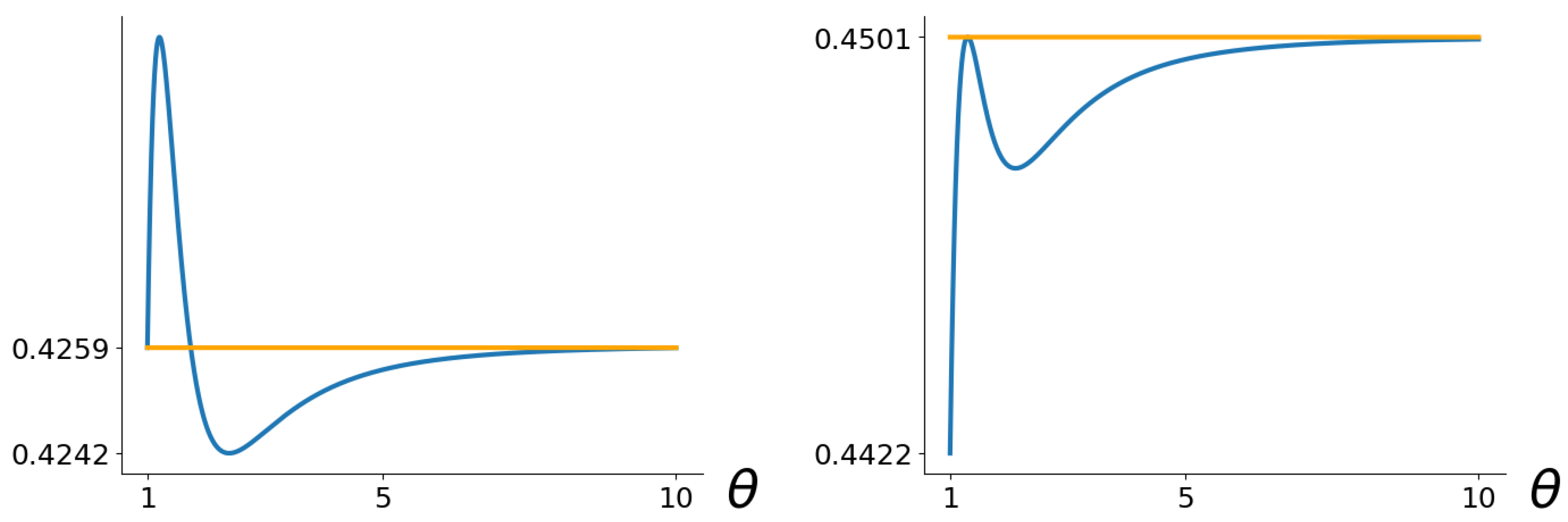
see Figure 4 (left). On the other hand, since $\psi \left(\theta \right)$ converges to its limit $\psi (\infty )$ from below (see Remark 9), from (ii) it follows that

$$\underset{1\le \mathsf{\Theta }\le \mathsf{\Theta }}{max}\psi \left(\theta \right)<\psi (\infty ),$$

(112)

and hence (104) implies

$$\underset{x\to \infty }{lim}{x}^{-1}{W}_{S,U}\left(x;x/x_S(\infty ),\infty \right)>\underset{x\to \infty }{lim}{x}^{-1}\underset{1\le \theta \le \mathsf{\Theta }}{max}{W}_{S,U}\left(x;x/x_S\left(\theta \right),\theta \right).$$

(113)

Combining (111) and (113), we see that there is an intermediate value $x_b>x^{**}$ where

$$W_{S,U}\left(x_b;x_b/x_S(\infty ),\infty \right)=\underset{1\le \theta \le \mathsf{\Theta }}{max}{W}_{S,U}\left(x_b;x_b/x_S\left(\theta \right),\theta \right),$$

(114)

see Figure 4 (right). Moreover, due to (100),

$$r{\displaystyle \frac{d}{dx}}\left(W_{S,U}\left(x;x/x_S\left(\theta \right),\theta \right)\right)=\psi \left(\theta \right),$$

which combined with (112) and (114) implies (110). □

The next statement uses the value $x_b$ defined in Proposition 7.

Proposition 8.

From (i)–(iii) it follows that:

• If $x\le x^{*}$, then the firm’s optimal policy is $\widehat{p}=x^{*}$ and $\widehat{\theta }=1$, i.e., $\xi =0$.
• If $x^{*}<x\le x_b$, then the firm’s optimal policy $(\widehat{p},\widehat{\theta })$ satisfies $1<\widehat{\theta }\le \mathsf{\Theta }$ (cf. (103)),

  $${\displaystyle \frac{d}{d\theta }}\left(W_{S,U}(x;x/x_S\left(\widehat{\theta }\right),\widehat{\theta })\right)=0,$$

  (115)

  and $\widehat{p}=x/x_S\left(\widehat{\theta }\right)$.
• If $x>x_b$, then the firm’s optimal policy is $\widehat{p}=x\gamma /(\gamma -1)$, $\widehat{\theta }=\infty$, i.e., $\xi =x\gamma {\sigma }^2/\left(2r(\gamma -1)\right)$.

Remark 11.

Using the initial state $X_0=x$ as a parameter, the value $x=x_b$ defined in Proposition 7 marks a shift in the firm’s optimal strategy. As x increases, at this point the firm’s optimal controls, the flow rate $\widehat{p}$ and the cancellation cost $\widehat{\xi }$, jump from the values

$$\widehat{p}(x_b-)={\displaystyle \frac{x_b}{x_S\left({\widehat{\theta }}_b\right)}},\widehat{\xi }(x_b-)={\displaystyle \frac{2x_b\epsilon \left({\widehat{\theta }}_b\right)}{x_S\left({\widehat{\theta }}_b\right){\sigma }^2}}$$

with ${\widehat{\theta }}_b$ satisfying $1<{\widehat{\theta }}_b\le \mathsf{\Theta }$ (cf. (103)) to the values

$$\widehat{p}(x_b+)={\displaystyle \frac{\gamma x_b}{\gamma -1}}<p(x_b-),\widehat{\xi }(x_b-)={\displaystyle \frac{\gamma x_b}{(\gamma -1)r}}$$

corresponding to $\theta =\infty$. Accordingly, the consumer changes their strategy from the two-threshold enrollment policy with the enrollment threshold $X_S=x_b$ and the cancellation threshold $X_U=x_b/\widehat{\theta }$ to the no-cancellation policy with the enrollment threshold $X_S=x_b$ and $X_U=0$. At the same time, the value function is continuous.

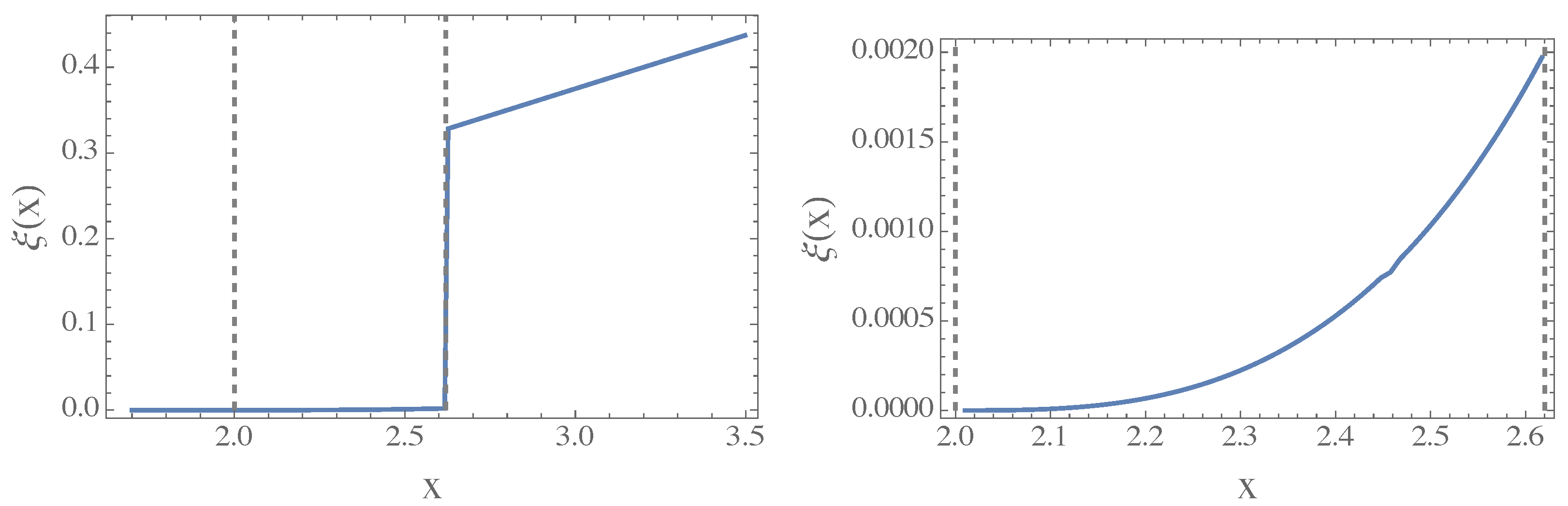
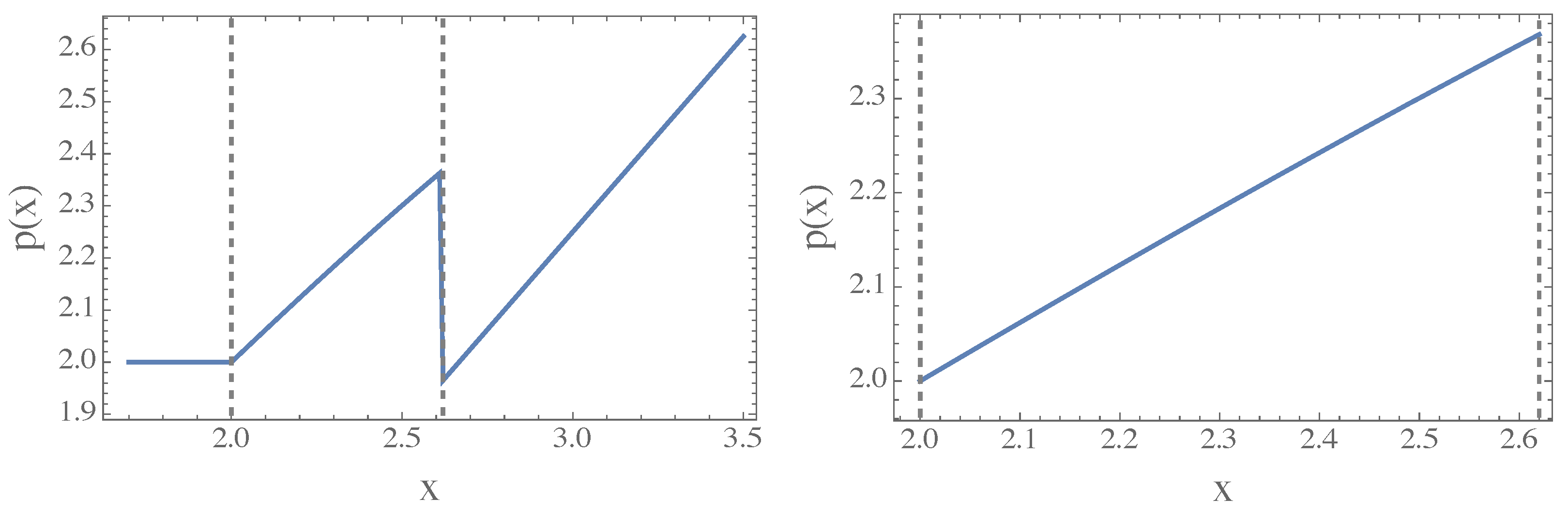
Figure 5 and Figure 6 present an example of the optimal controls $\widehat{\xi }\left(x\right),\widehat{p}\left(x\right)$. The optimal cancellation cost $\widehat{\xi }\left(x\right)$ is zero, and the optimal flow cost $\widehat{p}\left(x\right)=x^{*}=2$ is constant for all $x<x_{*}=2$. The point $x=x^{*}$ marks a continuous transition to the regime with a positive optimal cancellation cost. Both $\widehat{\xi }\left(x\right)$ and $\widehat{p}\left(x\right)$ grow non-linearly with x on the interval $2=x_{*}<x<x_b=2.62$ as shown in the right panels of Figure 5 and Figure 6 (the function $\widehat{p}\left(x\right)$ is almost, but not exactly, linear on this interval). The second transition point at $x=x_b=2.62$ marks a transition to the no-cancellation regime; this is a discontinuity point for both controls. At this point, the firm increases the cancellation cost and simultaneously decreases the flow cost of the subscription as shown in the left panels of Figure 5 and Figure 6. The consumer responds by setting $X_U=0$. In the no-cancellation domain, i.e., for all $x\ge x_b=2.62$, both controls $\widehat{\xi }$, $\widehat{p}$ are proportional to x.

Remark 12.

Remark 7 implies that the consumer responds to the flow rate p and the cancellation cost ξ set by the firm according to Propositions 8 with the single-threshold switching policy if $x\le x^{*}$ (the costless cancellation case), the two-threshold switching policy if $x^{*}<x\le x_b$, and the no-cancellation policy if $x>x_b$. If $x<x^{*}$, the consumer is initially unsubscribed; otherwise, the consumer subscribes at the initial instant. If $x\ge x^b$, the consumer never cancels the subscription.

Proof of Proposition 8.

If $p{x}_S\left(\theta \right)<x<p(\gamma -1)/\gamma$, then (as in the case $c=0$) the function $W=W_S$ increases in $\theta$ due to (99) and (i), hence the maximum of $W_S$ for a fixed p is achieved at $x=p{x}_S\left(\theta \right)$. If $x\ge p(\gamma -1)/\gamma$, then the maximum for a fixed p is achieved in the limit $\theta \to \infty$, hence $W_S(x;p,\infty )=p-c$ implies ${sup}_{p,\theta }\{W_S(x;p,\theta ):x\ge p(\gamma -1)/\gamma \}=W_S(x;x\gamma /(\gamma -1),\infty )$. On the other hand, $W_U$ satisfies $W_U(x;c,\theta )=W_U(x;\infty ,\theta )=0$ and has a unique local (and global) maximum on the interval $p\ge c$ at the point $p=x^{*}=c\delta /(\delta -1)$ for any fixed $x,\theta$. Therefore:

• if $x\le x^{*}$, then (88) implies that W achieves its maximum on the line $p=x^{*}$;
• if $x^{*}<x<x^{**}$, then W achieves its maximum on the curve

  $$p=max\{x/x_S\left(\theta \right),x^{*}\}=\left\{\begin{array}{cc}x/x_S\left(\theta \right),& 1\le \theta \le {\theta }_{*},\hfill \\ x^{*},& \theta >{\theta }_{*},\hfill \end{array}\right.$$

  (116)

  with ${\theta }_{*}$ defined by

  $$x_S\left({\theta }_{*}\right)={\displaystyle \frac{x}{x^{*}}}={\displaystyle \frac{x(\delta -1)}{c\delta }};$$

  (117)
• if $x\ge x^{**}$, then W achieves its maximum on the curve $p=x/x_S\left(\theta \right)$.

We note that $W=W_U$ on each of the above curves. Therefore, Relations (99) and (iii) imply that in the case $x\le x^{*}$ the firm’s optimal policy is $\widehat{p}=x^{*}$ and $\widehat{\theta }=1$. On the other hand, in the case $x\ge x^{**}$, Proposition 7 implies that if $x>x_b$, then $\widehat{p}=x\gamma /(\gamma -1)$ and $\widehat{\theta }=\infty$; if $x^{**}\le x\le x_b$, then $W_{S,U}\left(x;x/x_S(·),·\right)$ achieves its maximum in the interval $1\le \theta \le \mathsf{\Theta }$, hence the optimal policy satisfies (115); moreover, it satisfies $1<\widehat{\theta }\le \mathsf{\Theta }$ because

$$\underset{\theta \to 1}{lim}{\displaystyle \frac{d}{d\theta }}\left(W_{S,U}(x;x/x_S\left(\theta \right),\theta )\right)>0$$

(118)

due to (101). Finally, in the case $x^{*}<x<x^{**}$, the payoff on the curve (116) equals

$$W=\left\{\begin{array}{cc}{W}_{S,U}\left(x;x/x_S\left(\theta \right),\theta )\right),\hfill & 1\le \theta \le {\theta }_{*},\hfill \\ W_U(x;x^{*},\theta ),\hfill & \theta >{\theta }_{*}.\hfill \end{array}\right.$$

(119)

Therefore, Relations (105) with $\theta ={\theta }_{*}$ combined with (iii), (99) and (118) imply that W achieves its global maximum at a point $\widehat{\theta }\in (1,{\theta }_{*})$ and (115) holds. □

Remark 13.

One can show that the graph of $W_U(x;x^{*},·)$ lies above the graph of $W_{S,U}\left(x;x/x_S(·),·\right)$ with one intersection point at $\theta ={\theta }_{*}$ (cf. (119)) for any $x^{*}<x<x^{**}$; see the red and blue curves, respectively, on the right panel of Figure 3.

5. Firm Problem: Heterogeneous Market

Let us consider the market of consumers indexed by $\rho >0$ with $\rho$-dependent payoff (37) as in Section 2.3. Formula (37) implies that, given p and $\xi$ (as set by the firm), the parameter $\epsilon$ defined by (47) is the same for all the consumers. Hence, the parameter $\theta$ implicitly defined by (49) (cf. (51)) and the parameters $x_{S,U}$ given by (48) and $x_U={\theta }^{-1}{x}_S$ are also the same for all $\rho$. On the other hand, the switching thresholds of a consumer indexed by a particular $\rho$ are given by $X_{S,U}^{\rho }=p{x}_{S,U}\left(\theta \right)/\rho$. As such, the corresponding payoff derived by the firm from a subscription indexed by a particular $\rho$ equals

$$W(x;p,\theta )={\displaystyle \frac{p-c}{r}}·\left\{\begin{array}{cc}{\displaystyle 1-\omega \left(\theta \right){\left(\frac{x\rho }{p{x}_S\left(\theta \right)}\right)}^{\gamma },}\hfill & p{x}_S\left(\theta \right)<x\rho ,\hfill \\ {\displaystyle \left(1-\omega \left(\theta \right)\right){\left(\frac{x\rho }{p{x}_S\left(\theta \right)}\right)}^{\delta },}\hfill & p{x}_S\left(\theta \right)\ge x\rho ,\hfill \end{array}\right.$$

(cf. (88) and (89)). Integrating, the total firm’s payoff is given by

$$W(x;p,\theta )={\displaystyle \frac{p-c}{r}}\left(\left(1-\omega \left(\theta \right)\right){\left({\displaystyle \frac{x}{p{x}_S\left(\theta \right)}}\right)}^{\delta }{\int }_0^{p{x}_S\left(\theta \right)/x}{\rho }^{\delta }dF\left(\rho \right)\right.$$

(120)

$$\phantom{mmmmmmmm}+\left.{\int }_{p{x}_S\left(\theta \right)/x}^{\infty }dF\left(\rho \right)-\omega \left(\theta \right){\left({\displaystyle \frac{x}{p{x}_S\left(\theta \right)}}\right)}^{\gamma }{\int }_{p{x}_S\left(\theta \right)/x}^{\infty }{\rho }^{\gamma }dF\left(\rho \right)\right).$$

As a case study, let us assume the gamma distribution for $\rho$. By inspection, in this case (120) implies

$$W(x;p,\theta )={\displaystyle \frac{p-c}{r\mathsf{\Gamma }\left(\alpha \right)}}\left(\mathsf{\Gamma }(\alpha ,v)-\omega \left(\theta \right)v^{-\gamma }\mathsf{\Gamma }(\alpha +\gamma ,v)+\left(1-\omega \left(\theta \right)\right)v^{-\delta }\left(\mathsf{\Gamma }(\alpha +\delta )-\mathsf{\Gamma }(\alpha +\delta ,v)\right)\right),$$

(121)

where $\omega \left(\theta \right)$ is given by (89), $\alpha >-\gamma$, $\beta >0$ are the parameters of the gamma distribution and

$$v={\displaystyle \frac{\beta p{x}_S\left(\theta \right)}{x}}.$$

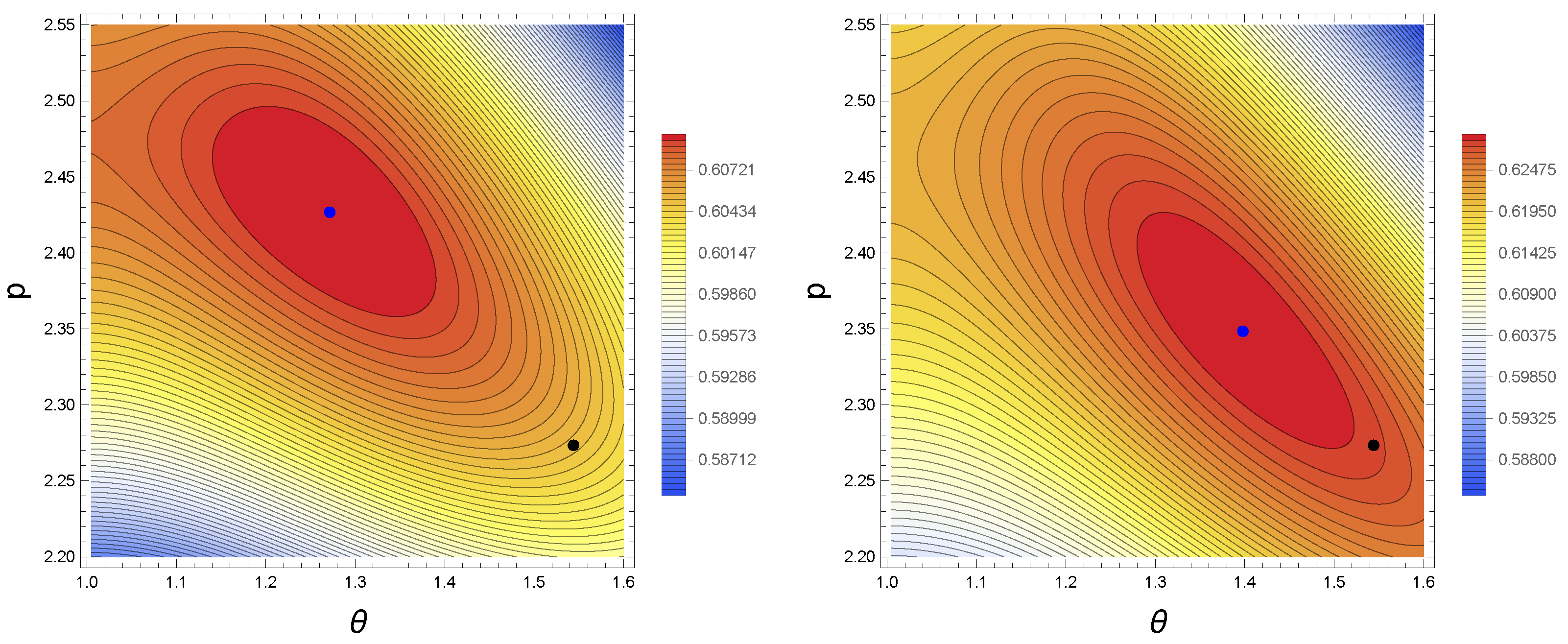
Figure 7 presents a contour plot of the payoff function (120) on the $(\theta ,p)$-plane for two sets of parameters $(\alpha ,\beta )$ of the gamma distribution. In both cases, $\alpha =\beta$, hence the mean of gamma distribution equals one. The parameter $\alpha =\beta$ is greater for the right plot, corresponding to a smaller variance. The blue dot is the maximizer $({\widehat{\theta }}_{\alpha },{\widehat{p}}_{\alpha })$ of (120). The black dot is the maximizer $(\widehat{\theta },\widehat{p})$ of the firm’s payoff (88) in the homogeneous market, i.e., the optimal solution of the firm’s problem with a single representative consumer. The parameters $\delta ,\gamma ,c,x$ correspond to the case $x^{*}<x\le x_b$ of Proposition 8 where this optimal solution places the enrollment threshold at the point $X_S=\widehat{p}{x}_S\left(\widehat{\theta }\right)=x$, hence the consumer subscribes at the initial instant. In the distributed model (120) of the heterogeneous market, the consumers with the enrollment threshold $X_S\left(\rho \right)={\widehat{p}}_{\alpha }{x}_S\left({\widehat{\theta }}_{\alpha }\right)/\rho \le x$ are subscribed at the initial instant, while the consumers with $X_S\left(\rho \right)={\widehat{p}}_{\alpha }{x}_S\left({\widehat{\theta }}_{\alpha }\right)/\rho >x$ are initially unsubscribed, and will enroll later. As expected, the maximizer of the distributed model approaches the maximizer of the firm’s problem with a single consumer as the variance $\alpha /{\beta }^2=1/\alpha$ of the gamma distribution decreases (the blue and black dots are closer on the right panel); the maximizers are expected to coalesce in the limit $\alpha \to \infty$ ensuring that $({\widehat{\theta }}_{\alpha },{\widehat{p}}_{\alpha })\to (\widehat{\theta },\widehat{p})$ in this limit. Moreover, the optimal strategy payoff $W(x;{\widehat{p}}_{\alpha },{\widehat{\theta }}_{\alpha })$ increases with the decreasing variance.

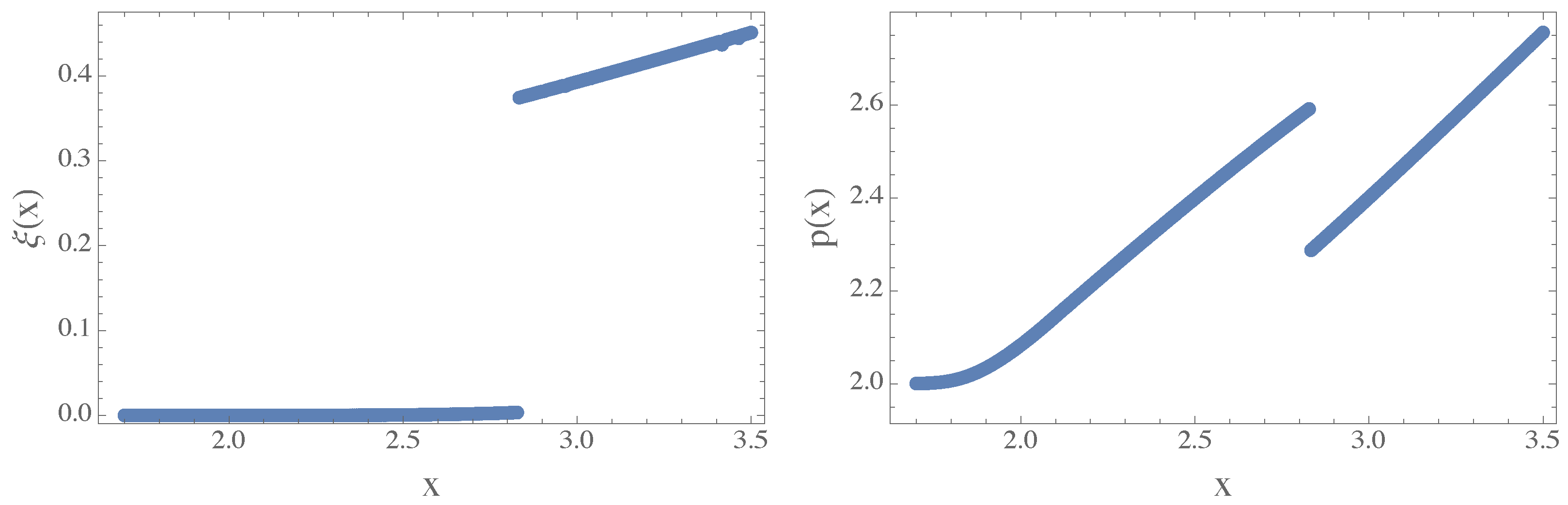
The discontinuity in the dependence of the optimal controls $\widehat{\xi }\left(x\right)$, $\widehat{p}\left(x\right)$ on the initial state x persists under heterogeneity; see Figure 8. The optimal flow cost $\widehat{p}$ of subscription is higher than for the homogeneous market (cf. Figure 6). This is consistent with Figure 7.

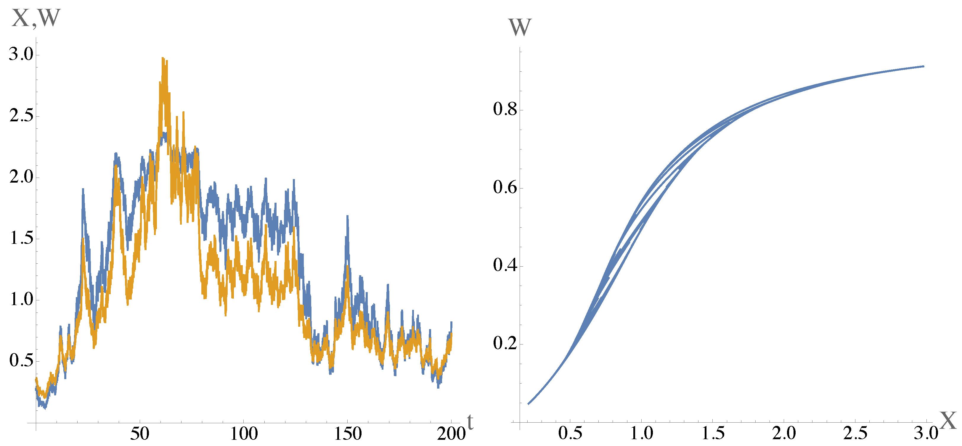
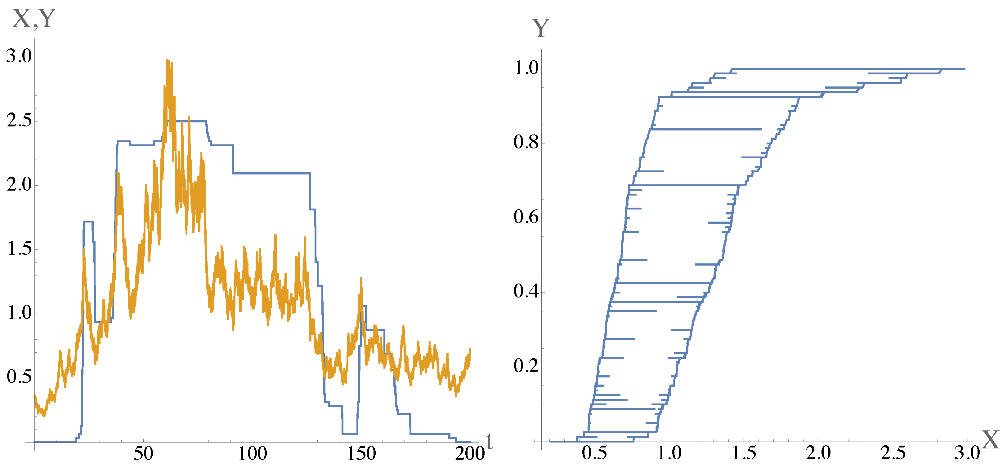
The firm’s expected payoff $W_t$ and flow revenue $Y_t$ demonstrate distinctive features of history dependence, which are typical of the output of the Preisach operator; see Figure 9 and Figure 10 where the yellow plot is a sample state trajectory $X_t$. In particular, the values of $W_t$ (the blue plot in Figure 9, left)over the time interval $80\le t\le 130$ after the global peak of $X_t$ are consistently higher than the values of $W_t$ around the time $t=40$ preceding the peak of $X_t$, while $X_t$ has approximately the same value during these times. In other words, $X_t$ returns to the same value after the peak but $W_t$ has higher values after the peak than before. This effect is eliminated only after $t=140$ when the value $X_t$ drops very low (the so-called wiping out property of the Preisach history dependence [19]). The same features are even more pronounced in the left panel of Figure 10 showing the plot of $Y_t$ (blue) for the same sample state trajectory $X_t$. The right panels of Figure 9 and Figure 10 show hysteresis loops on the plane $(X,W)$ and $(X,Y)$, respectively. As a manifestation of history dependence, $W_t$ has different values for the same value of $X_t$ achieved at different times; the same is true for $Y_t$.

6. Conclusions

We formulated a stochastic optimal control model of a subscription economy with cancellation costs. The consumer’s problem is equivalent to the classical real-options model of entry and exit under uncertainty with adjustment costs and admits a two-threshold solution with an inaction band and hysteresis. We derived an explicit parametric representation of this solution, transforming the standard implicit characterization by a nonlinear free-boundary system into closed-form expressions for the switching thresholds and cancellation cost.

In a homogeneous market with a representative consumer, the firm’s optimal policy partitions the state space into three regimes. For small initial utility levels, the optimal cancellation cost is zero and the subscription fee remains constant over a range of states. In an intermediate regime, both controls depend nontrivially on the state, and the firm’s optimal policy induces the consumer to choose an entry threshold equal to the initial utility level, thereby ensuring immediate subscription. For sufficiently large utility levels, the firm induces an effective permanent lock-in effect: the consumer subscribes immediately and never subsequently unsubscribes. The transition between the latter two regimes is discontinuous and reflects a competition between two local maxima of the firm’s payoff function. These results yield several qualitative predictions. For low utility levels, firms have little incentive to impose cancellation costs. As utility increases, so does the cancellation cost, and the gap between the subscription and cancellation thresholds widens, resulting in more pronounced hysteresis and consumer inertia. For sufficiently high utility levels, the optimal policy switches discontinuously to a permanent lock-in regime characterized by a high cancellation cost and a low subscription fee.

We then extended the model to a heterogeneous population of consumers with different utility coefficients. The superposition of individual two-threshold subscription strategies gives rise to the Preisach hysteresis operator, which describes the aggregate dependence of the firm’s revenue on the utility dynamics. As in the homogeneous setting, the explicit parametric representation of the Dixit entry–exit solution reduces the firm’s optimization problem to unconstrained optimization over a two-dimensional parameter space. The discontinuous transition between payoff maximizing regimes persists under heterogeneity, demonstrating the robustness of the underlying mechanism.

The Preisach representation further implies complex history dependence in the firm’s flow revenue and expected payoff. In particular, temporary positive and negative shocks to consumer utility may have long-lasting effects on future revenues because the composition of subscribed and unsubscribed consumers depends on the past evolution of the utility process. Similar ideas arise in macroeconomic models of hysteresis, where temporary shocks can induce persistent changes in employment and output [11]. For the case of a gamma distribution of consumer preferences, we obtained explicit expressions for the firm’s revenue and expected payoff in terms of incomplete gamma functions.

The present model is intentionally stylized. In particular, the subscription price is assumed to remain fixed throughout the planning horizon; a more realistic formulation would allow for periodic subscription renewals and dynamic pricing policies that adapt to observed consumer behavior and demand estimates [41]. Likewise, the utility process is modeled as a geometric Brownian motion for analytical tractability and consistency with the classical real-options literature. Extensions to mean-reverting or bounded state dynamics, as well as closed-loop models in which subscription revenues affect future utility through investment decisions, would provide a more realistic description of consumer behavior. More generally, one may consider coupled economic-dynamical systems in which economic decisions and state variables evolve jointly [42].

References

1. Subscription Service Statistics and Costs. C+R Research Report. 2024. Available online: https://www.crresearch.com/blog/subscription-service-statistics-and-costs/ (accessed on 7 March 2026).
2. Chen, C.Q. Literature Review and Theoretic Critique to the Research of Subscription Sales. 2024. Available online: https://ssrn.com/abstract=5005389 (accessed on 7 March 2026).
3. Libai, B.; Muller, E.; Schoenmueller, V. The effects of churn on the growth of subscription services. Int. J. Res. Mark. 2026, 43, 92–112. [Google Scholar]
4. Lariviere, J.; Lu, C.H. Welfare Impacts of Subscriptions for Digital Goods: The Case of Video Games. 2024. Available online: https://www.researchgate.net/profile/Carol-Hengheng-Lu/publication/378398479_Welfare_Impacts_of_Subscriptions_for_Digital_Goods_The_Case_of_Video_Games/links/65d80ef1adc608480ae0374a/Welfare-Impacts-of-Subscriptions-for-Digital-Goods-The-Case-of-Video-Games.pdf (accessed on 7 March 2026).
5. Einav, L.; Klopack, B.; Mahoney, N. Selling subscriptions. Am. Econ. Rev. 2025, 115, 1650–1671. [Google Scholar] [CrossRef]
6. Xu, L.; Sun, Y.; Hsu, Y.-T.; Chiu, Y.-L. The effects of personalized recommendations on perceived switching costs: The mediation roles of customer satisfaction and habits. Electron. Mark. 2025, 35, 80. [Google Scholar] [CrossRef]
7. FTC Final Click-to-Cancel Rule. 2024. Available online: https://www.ftc.gov/news-events/news/press-releases/2024/10/federal-trade-commission-announces-final-click-cancel-rule-making-it-easier-consumers-end-recurring/ (accessed on 7 March 2026).
8. Dixit, A. Entry and exit decisions under uncertainty. J. Political Econ. 1989, 97, 620–638. [Google Scholar] [CrossRef]
9. Dixit, A.K.; Pindyck, R.S. Investment Under Uncertainty; Princeton University Press: Princeton, NJ, USA, 1994. [Google Scholar]
10. McDonald, R.; Siegel, D. The value of waiting to invest. Q. J. Econ. 1986, 101, 707–728. [Google Scholar] [CrossRef]
11. Cross, R.; Darby, J.; Ireland, J.; Piscitelli, L. Hysteresis and unemployment: A preliminary investigation. In The Science of Hysteresis; Bertotti, G., Mayergoyz, I., Eds.; Elsevier: Amsterdam, The Netherlands, 2006; Volume 1, pp. 667–699. [Google Scholar]
12. Vintila, N. Entry and exit decisions under uncertainty: A real option approach. Theor. Appl. Econ. 2008, 11, 341–348. [Google Scholar]
13. Visintin, A. Differential Models of Hysteresis; Springer: Berlin/Heidelberg, Germany, 1994. [Google Scholar]
14. Dias, J.; Larguinho, M.; Braumann, C. Entry and exit decisions under uncertainty for a generalized class of one-dimensional diffusions. In Proceedings of the Real Options Conference, Athens, Greece, 17–20 June 2015. [Google Scholar]
15. Arthur, W.B. Competing technologies, increasing returns, and lock-in by historical events. Econ. J. 1989, 99, 116–131. [Google Scholar] [CrossRef]
16. Farrell, J.; Klemperer, P. Coordination and lock-in: Competition with switching costs and network effects. Handb. Ind. Organ. 2007, 3, 1967–2072. [Google Scholar] [CrossRef]
17. Bertotti, G.; Mayergoyz, I. (Eds.) The Science of Hysteresis; Elsevier: Amsterdam, The Netherlands, 2006; Volume 1–3. [Google Scholar]
18. Rachinskii, D.; Rachinskiy, L.; Rivera, A. Foundations of the Preisach operator in real options problems with subscription cost and heterogeneous population of consumers. Axioms 2025, 14, 829. [Google Scholar] [CrossRef]
19. Mayergoyz, I.D. Mathematical Models of Hysteresis and Their Applications: Electro-Magnetism; Academic Press: Cambridge, MA, USA, 2003. [Google Scholar]
20. Bensoussan, A.; Lions, J.-L. Applications of Variational Inequalities in Stochastic Control; Elsevier: Amsterdam, The Netherlands, 1982. [Google Scholar]
21. Bensoussan, A.; Lions, J.-L. Impulse Control and Quasi-Variational Inequalities; Willey: Hoboken, NJ, USA, 1987. [Google Scholar]
22. Acharya, S.; Bensoussan, A.; Rachinskii, D.; Rivera, A. Real options problem with nonsmooth obstacle. SIAM J. Financ. Math. 2021, 12, 1508–1552. [Google Scholar] [CrossRef]
23. Bensoussan, A.; Chevalier-Roignant, B.; Rivera, A. Does performance-sensitive debt mitigate debt overhang? J. Econ. Dyn. Control 2021, 131, 104203. [Google Scholar] [CrossRef]
24. Preisach, F. Über die magnetische Nachwirkung. Z. Phys. 1935, 94, 277–302. [Google Scholar] [CrossRef]
25. Krasnosel’skii, M.A.; Pokrovskii, A.V. Systems with Hysteresis; Springer: Berlin/Heidelberg, Germany, 1989. [Google Scholar]
26. Krejčí, P.; Kuhnen, K. Inverse control of systems with hysteresis and creep. IEE Proc.-Control Theory Appl. 2001, 148, 185–192. [Google Scholar] [CrossRef]
27. Al-Bender, F.; Lampaert, V.; Swevers, J. The generalized Maxwell-slip model: A novel model for friction simulation and compensation. IEEE Trans. Autom. Control 2005, 50, 1883–1887. [Google Scholar] [CrossRef]
28. Ruderman, M.; Rachinskii, D. Use of Prandtl-Ishlinskii hysteresis operators for Coulomb friction modeling with presliding. J. Phys. Conf. Ser. 2017, 811, 012013. [Google Scholar] [CrossRef]
29. Haverkamp, R.; Reggiani, P.; Rossand, P.J.; Parlange, J.-Y. Soil water hysteresis prediction model based on theory and geometric scaling. In Environmental Mechanics: Water Mass and Energy Transfer in the Biosphere; Raats, P.A.C., Smiles, D., Warrick, A.W., Eds.; American Geophysical Union: Washington, DC, USA, 2002; pp. 213–246. [Google Scholar]
30. Apicella, V.; Clemente, C.S.; Davino, D.; Leone, D.; Visone, C. Review of modeling and control of magnetostrictive actuators. Actuators 2019, 8, 45. [Google Scholar] [CrossRef]
31. Balanov, Z.; Krawcewicz, W.; Rachinskii, D.; Zhezherun, A. Hopf bifurcation in symmetric networks of coupled oscillators with hysteresis. J. Dyn. Differ. Equ. 2012, 24, 713–759. [Google Scholar] [CrossRef]
32. Iyer, R.V.; Tan, X.; Krishnaprasad, P.S. Approximate inversion of the Preisach hysteresis operator with application to control of smart actuators. IEEE Trans. Autom. Control 2005, 50, 798–810. [Google Scholar] [CrossRef]
33. Al Janaideh, M.; Rakheja, S.; Su, C.Y. An analytical generalized Prandtl–Ishlinskii model inversion for hysteresis compensation in micropositioning control. IEEE/ASME Trans. Mechatron. 2010, 16, 734–744. [Google Scholar] [CrossRef]
34. Tan, X.; Baras, J.S. Modeling and control of hysteresis in magnetostrictive actuators. Automatica 2004, 40, 1469–1480. [Google Scholar] [CrossRef]
35. Mayergoyz, I.D.; Korman, C. Hysteresis and Neural Memory; World Scientific: Singapore, 2019. [Google Scholar]
36. Kopfová, J.; Nábělková, P.; Rachinskii, D.; Rouf, S. Dynamics of SIR model with vaccination and heterogeneous behavioral response of individuals modeled by the Preisach operator. J. Math. Biol. 2021, 83, 11. [Google Scholar] [CrossRef] [PubMed]
37. Guan, R.; Kopfová, J.; Rachinskii, D. Global stability of SIR model with heterogeneous transmission rate modeled by the Preisach operator. SIAM J. Appl. Dyn. Syst. 2024, 23, 1199–1241. [Google Scholar] [CrossRef]
38. Adamonis, J.; Göcke, M. Modeling economic hysteresis losses caused by sunk adjustment costs. J. Post Keynes. Econ. 2019, 42, 299–318. [Google Scholar]
39. Rios, L.A.; Rachinskii, D.; Cross, R. A model of hysteresis arising from social interaction within a firm. J. Phys. Conf. Ser. 2017, 811, 012011. [Google Scholar] [CrossRef]
40. Werner, L.M. Hysteresis losses in the Preisach framework. Empir. Econ. 2018, 58, 1249–1278. [Google Scholar] [CrossRef]
41. Hanono-Gómez, M.; López-Barrientos, J.D.; Rodríguez-Carreon, C.; Kalashnykova, N. Retail pricing optimization with Monte Carlo Tree Search. In Digital Synergy; El Emary, I.M.M., Brzozowska, A., Maśloch, P., Eds.; CRC Press: Boca Raton, FL, USA, 2024; Volume Chapter 25, pp. 218–225. [Google Scholar]
42. Shah, S.M.A.; Gang, P.; Alkhazzan, A. A stochastic epidemic-economic model: Threshold dynamics and stability analysis. Eur. Phys. J. Plus 2026, 141, 414. [Google Scholar] [CrossRef]
Figure 1. Consumer’s thresholds as functions of the cancellation cost ξ . The horizontal asymptote of x S corresponds to θ , the range of ξ corresponds to 1 < θ < (equivalently, 0 < ε < 1 / ( δ γ ) ), cf. (65). The parameters are δ = 2 , γ = 3 .
Axioms 15 00506 g001
Figure 2. Typical plots of the functions ϕ ( θ ) (left) and ψ ( θ ) (right) defined in (98); the yellow line is the horizontal asymptote γ / ( γ 1 ) of ψ as θ .
Axioms 15 00506 g002
Figure 3. Left: a typical plot of function φ ( θ ) defined in (98) and its horizontal asymptote ( γ / ( γ 1 ) ) δ as θ . Right: typical plots of functions θ δ γ θ δ θ δ γ 1 x S ( θ ) 1 χ (blue) and θ δ γ θ δ θ δ γ 1 χ δ x S ( θ ) δ 1 δ χ δ 1 (red) with χ = c / x for a fixed x ( x * , x * * ) . The intersection point θ * of these graphs is given by (117). The horizontal asymptotes as θ for the blue and red curves are γ / ( γ 1 ) χ and χ δ ( γ 1 ) ( δ 1 ) γ δ χ δ 1 , respectively. The red curve has the same profile on both panels up to a positive coefficient.
Axioms 15 00506 g003
Figure 4. A typical plot of the function r x 1 W S , U x ; x / x S ( θ ) , θ = θ δ γ θ δ θ δ γ 1 x S ( θ ) 1 χ with χ = c / x for x = x * * (left) and x = x b (right).
Axioms 15 00506 g004
Figure 5. Optimal control ξ ^ ( x ) for the homogeneous market (left). The left vertical dashed line at x = x * = 2 corresponds to the continuous transition from costless cancellation regime ( ξ ^ = 0 for x x * ) to the positive cancellation cost ( ξ ^ > 0 for x > x * ). The right vertical dashed line at x = x b = 2.62 corresponds to the discontinuous transition to the no-cancellation regime when the consumer responds to the high cancellation cost by setting X U = 0 for x > x b . The control ξ ^ is proportional to x for x > x b . The right panel zooms into the region x * < x < x b between the dashed lines. The parameters are c = 1 , δ = 2 , γ = 3 .
Axioms 15 00506 g005
Figure 6. Optimal control p ^ ( x ) for the homogeneous market (left). The transition points marked by the vertical dashed lines and the parameters are the same as in Figure 5. The control p ^ is constant on the interval x x * , proportional to x on the interval x > x b , and has a discontinuity at x = x b . The right panel zooms into the region x * < x < x b between the dashed lines.
Axioms 15 00506 g006
Figure 7. Contour plot of the payoff function (120) of the distributed model for α = β = 50 (left) and α = β = 200 (right). The maximum payoff value achieved at the blue point equals W ^ = 0.61 (left) W ^ = 0.63 (right). The maximizer of the payoff (88) of the single-consumer model is shown by the black dot, where this payoff achieves the value W ^ = 0.654 . The other parameters for both plots are δ = 2.65 , γ = 1.25 , c = 1 , x = 2.83 .
Axioms 15 00506 g007
Figure 8. Optimal controls ξ ^ ( x ) (left) and p ^ ( x ) (right) for the heterogeneous market with the gamma distributed consumer preferences. Parameters of the gamma distribution are α = β = 20 ; other parameters are the same as in Figure 5 and Figure 6.
Axioms 15 00506 g008
Figure 9. Left: Sample state trajectory X t (yellow) and the corresponding trajectory of the firm’s flow revenue (blue) for the model with N = 80 consumers. The distribution of the coefficient ρ of the consumer preferences (cf. (37)) is sampled from the gamma distribution with parameters α = β = 15 . Right: The corresponding hysteresis loops on the ( X , W ) plane. Parameters are δ = 1.5 , γ = 1.5 , σ = 0.15 , μ = 0.111 , r = 0.0025 .
Axioms 15 00506 g009
Figure 10. The trajectory Y t of the firm’s expected payoff (blue) for the state trajectory X t (yellow) from Figure 9 (left), and the corresponding hysteresis loops on the ( X , Y ) plane (right).
Axioms 15 00506 g010
Disclaimer/Publisher’s Note: The statements, opinions and data contained in all publications are solely those of the individual author(s) and contributor(s) and not of MDPI and/or the editor(s). MDPI and/or the editor(s) disclaim responsibility for any injury to people or property resulting from any ideas, methods, instructions or products referred to in the content.