Figure 1.
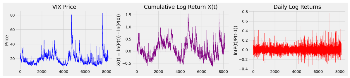
VIX over 1990–2026. (Left): Price level , with the 2008 (80.86) and COVID-19 (82.69) spikes visible. (Centre): Cumulative log-return , the quantity to which the partition function is applied. (Right): Daily log-returns , showing pronounced volatility clustering.
Figure 1.
VIX over 1990–2026. (Left): Price level , with the 2008 (80.86) and COVID-19 (82.69) spikes visible. (Centre): Cumulative log-return , the quantity to which the partition function is applied. (Right): Daily log-returns , showing pronounced volatility clustering.
Figure 2.
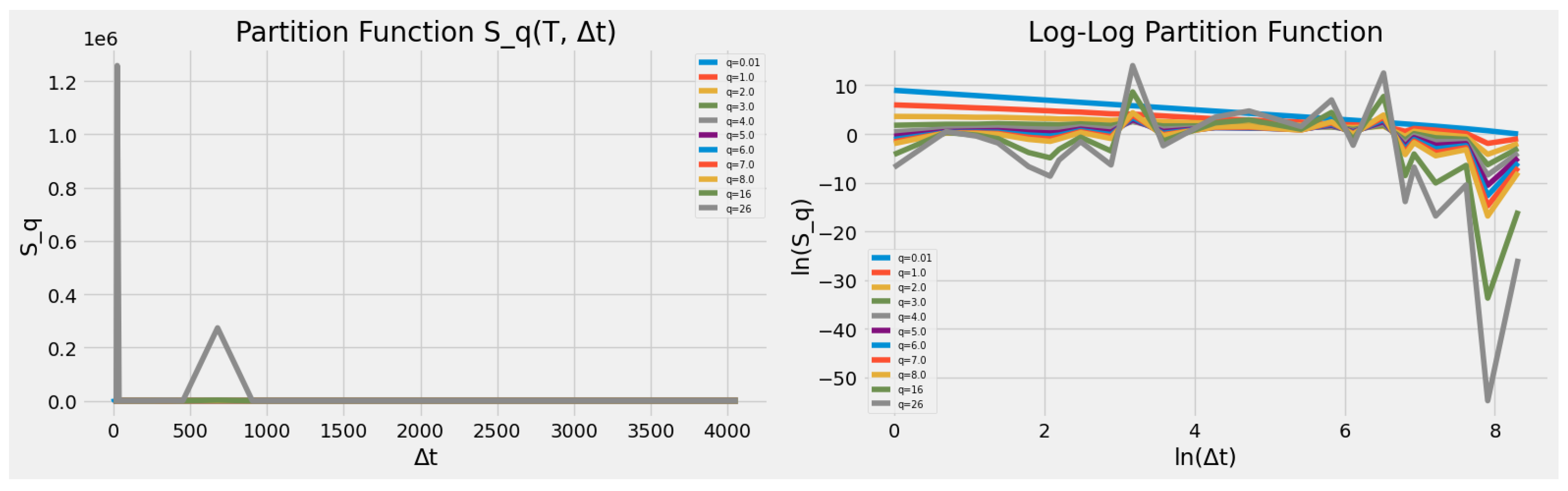
Partition function
(
Left) and its log–log transform (
Right) for representative moment orders
q. Approximate linearity of
in
is the scaling signature exploited in (
9). The visible jaggedness of the log–log traces reflects the irregular, unevenly spaced integer-divisor ladder of
(
Section 6.9).
Figure 2.
Partition function
(
Left) and its log–log transform (
Right) for representative moment orders
q. Approximate linearity of
in
is the scaling signature exploited in (
9). The visible jaggedness of the log–log traces reflects the irregular, unevenly spaced integer-divisor ladder of
(
Section 6.9).
Figure 3.
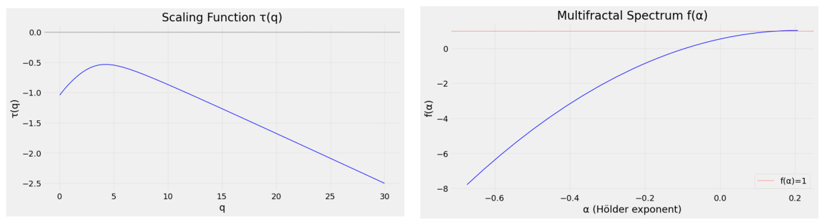
(
Left): Estimated scaling function
. Strict concavity (curvature
) is the lognormal-cascade signature and the defining condition for multifractality; a monofractal would give a straight line. (
Right): Multifractal (singularity) spectrum
obtained by Legendre transform (
11), peaking at
with
. Spectrum breadth quantifies the degree of multifractality.
Figure 3.
(
Left): Estimated scaling function
. Strict concavity (curvature
) is the lognormal-cascade signature and the defining condition for multifractality; a monofractal would give a straight line. (
Right): Multifractal (singularity) spectrum
obtained by Legendre transform (
11), peaking at
with
. Spectrum breadth quantifies the degree of multifractality.
Figure 4.
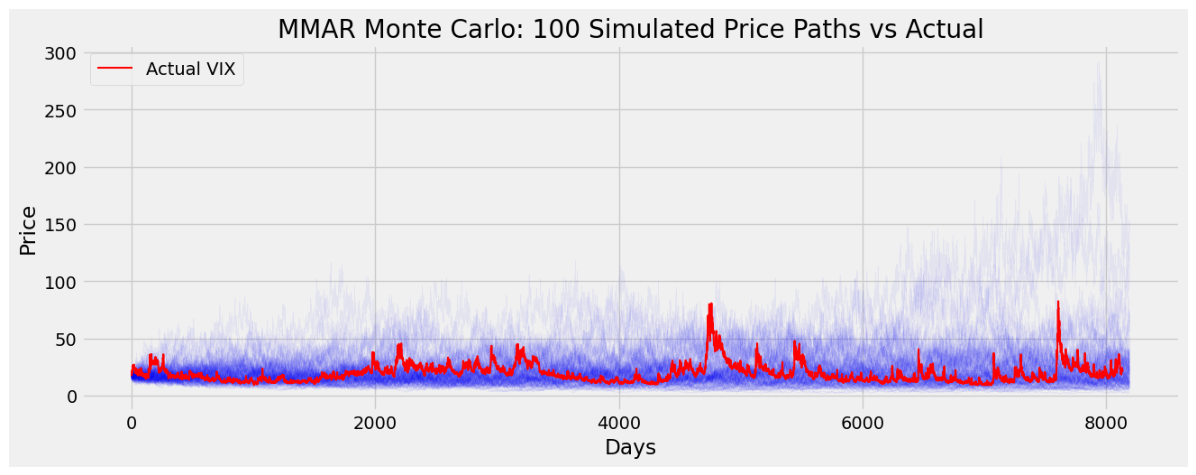
One hundred representative MMAR Monte Carlo price paths (blue, ) against the realised VIX (red). The simulated envelope reproduces the clustered-burst character of the index but rarely attains the most extreme realised peaks.
Figure 4.
One hundred representative MMAR Monte Carlo price paths (blue, ) against the realised VIX (red). The simulated envelope reproduces the clustered-burst character of the index but rarely attains the most extreme realised peaks.
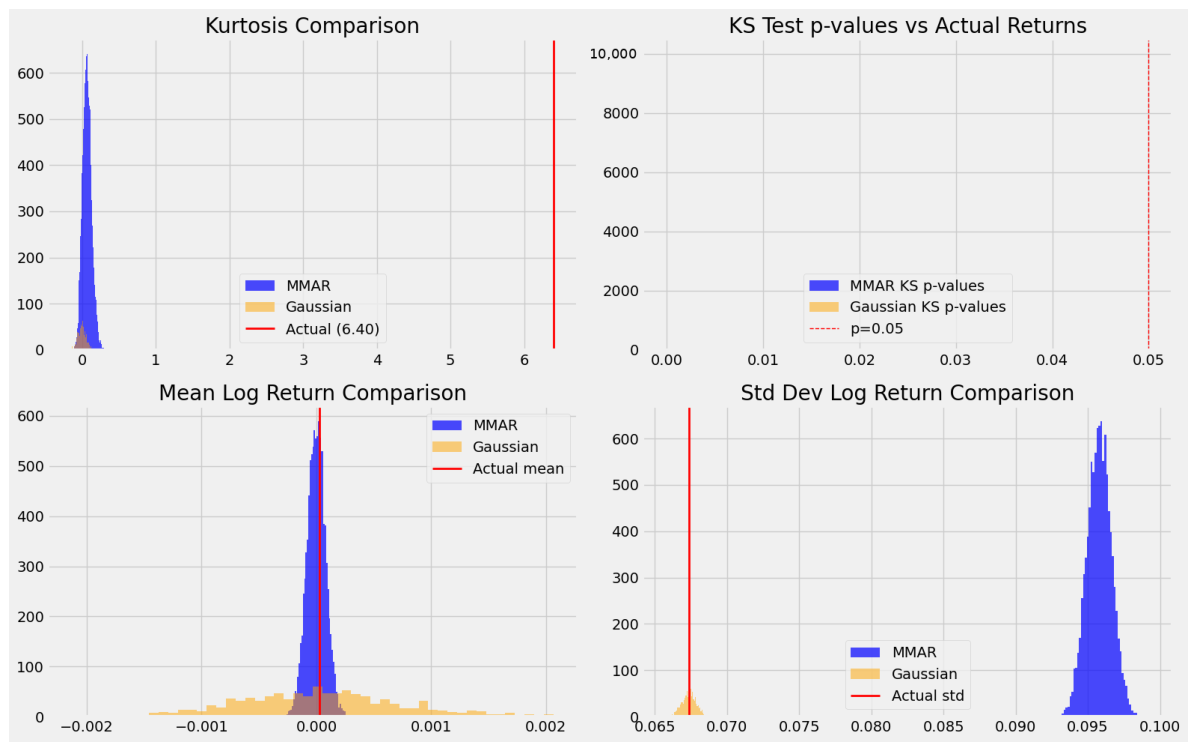
Figure 5.
MMAR vs. Gaussian benchmark across four moments of the simulated return distribution: Kurtosis, KS p-values against empirical returns, mean log-return, and standard deviation. MMAR (blue) concentrates near the empirical kurtosis far better than the Gaussian (orange), but neither reaches the empirical value (red line).
Figure 5.
MMAR vs. Gaussian benchmark across four moments of the simulated return distribution: Kurtosis, KS p-values against empirical returns, mean log-return, and standard deviation. MMAR (blue) concentrates near the empirical kurtosis far better than the Gaussian (orange), but neither reaches the empirical value (red line).
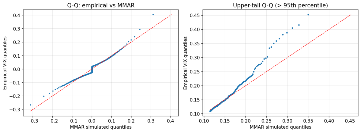
Figure 6.
Quantile–quantile plots of empirical VIX log-returns against pooled MMAR simulations. (Left): Full distribution; the flat segment near the origin reflects the over-peaked simulated centre. (Right): Upper tail beyond the 95th percentile; empirical quantiles rise increasingly above the line, the signature of the model’s tail under-dispersion.
Figure 6.
Quantile–quantile plots of empirical VIX log-returns against pooled MMAR simulations. (Left): Full distribution; the flat segment near the origin reflects the over-peaked simulated centre. (Right): Upper tail beyond the 95th percentile; empirical quantiles rise increasingly above the line, the signature of the model’s tail under-dispersion.
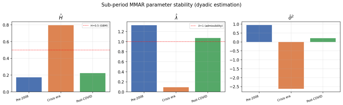
Figure 7.
Sub-period instability of , and . The crisis-era window violates both admissibility () and the subdiffusive classification (), in contrast to the full-sample estimates.
Figure 7.
Sub-period instability of , and . The crisis-era window violates both admissibility () and the subdiffusive classification (), in contrast to the full-sample estimates.
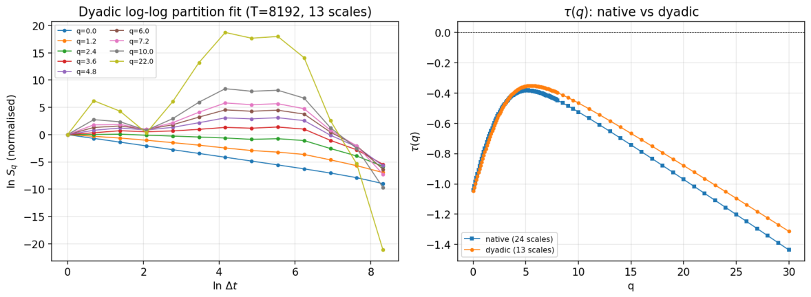
Figure 8.
(
Left): Log–log partition function on the 13 dyadic scales after resampling to
; the regressions are visibly cleaner than the 8-scale fit of
Figure 2. (
Right):
estimated on native integer-divisor scales vs. dyadic scales—both strictly concave, with modest divergence at high
q.
Figure 8.
(
Left): Log–log partition function on the 13 dyadic scales after resampling to
; the regressions are visibly cleaner than the 8-scale fit of
Figure 2. (
Right):
estimated on native integer-divisor scales vs. dyadic scales—both strictly concave, with modest divergence at high
q.
Figure 9.
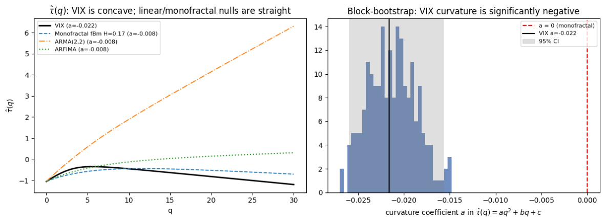
(Left): for VIX (solid, strongly concave) against a monofractal fBm, the best-fit ARMA(2,2), and an ARFIMA null—all of which remain close to linear. (Right): Stationary block-bootstrap distribution of the VIX curvature coefficient a; the interval excludes both zero and the ≈−0.008 baseline of the linear/monofractal nulls.
Figure 9.
(Left): for VIX (solid, strongly concave) against a monofractal fBm, the best-fit ARMA(2,2), and an ARFIMA null—all of which remain close to linear. (Right): Stationary block-bootstrap distribution of the VIX curvature coefficient a; the interval excludes both zero and the ≈−0.008 baseline of the linear/monofractal nulls.
Figure 10.
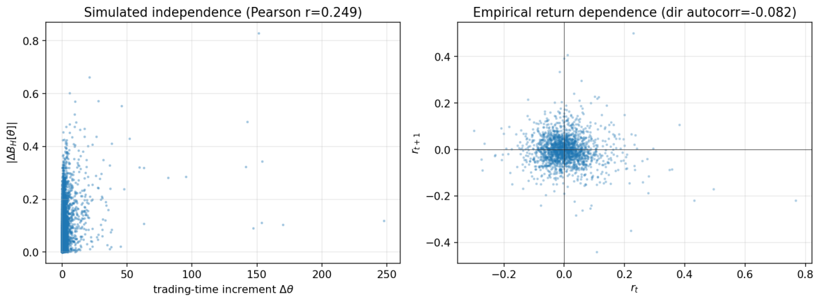
(Left): Simulated trading-time increments vs. ; the positive association is the subordination-induced clustering channel. (Right): Empirical return dependence vs. ; the weak negative directional autocorrelation, strengthening around spikes, is the exploratory signal that intensity and direction are not strictly independent.
Figure 10.
(Left): Simulated trading-time increments vs. ; the positive association is the subordination-induced clustering channel. (Right): Empirical return dependence vs. ; the weak negative directional autocorrelation, strengthening around spikes, is the exploratory signal that intensity and direction are not strictly independent.
Figure 11.
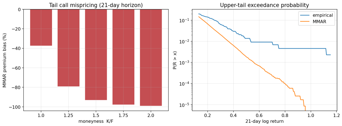
(Left): Relative MMAR mispricing of one-month calls by moneyness; the bias deepens monotonically out of the money. (Right): Upper-tail exceedance probability (log scale) for empirical vs. MMAR h-day returns—the empirical tail is far heavier, which is the source of the pricing gap.
Figure 11.
(Left): Relative MMAR mispricing of one-month calls by moneyness; the bias deepens monotonically out of the money. (Right): Upper-tail exceedance probability (log scale) for empirical vs. MMAR h-day returns—the empirical tail is far heavier, which is the source of the pricing gap.
Table 1.
Three empirical properties captured by MMAR.
Table 1.
Three empirical properties captured by MMAR.
| Property | Mechanism |
|---|
| Non-Gaussian distribution (fat tails) | Multiplicative cascade heterogeneity |
| Heteroskedasticity () | Fractional Brownian motion |
| Volatility clustering | Trading time CDF maps fast/slow periods |
Table 2.
MMAR parameter estimates for VIX (9144 daily obs., 1990–2026; native 24-scale estimation). renders the lognormal cascade fully identifiable.
Table 2.
MMAR parameter estimates for VIX (9144 daily obs., 1990–2026; native 24-scale estimation). renders the lognormal cascade fully identifiable.
| Parameter | Value | Interpretation |
|---|
| 0.1815 | Strongly anti-persistent fBm () |
| 0.2372 | Most probable Hölder exponent |
| 1.3066 | Cascade mean (>1: admissible) |
| | Cascade variance (admissible, >0) |
| b | 2 | Binomial cascade branching factor |
Table 3.
Monte Carlo validation: MMAR vs. GBM vs. empirical VIX.
Table 3.
Monte Carlo validation: MMAR vs. GBM vs. empirical VIX.
| Metric | MMAR | GBM | Empirical VIX |
|---|
| Mean excess kurtosis | 5.67 | | 6.75 |
| Mean log return | ≈0 | | |
| Mean SD of returns | 0.0680 | 0.0680 | 0.0680 |
| KS p-value (mean) | 0.000 | 0.000 | — |
| % paths KS | 0.0% | 0.0% | — |
Table 4.
KS rejection decomposed by region (pooled MMAR vs. empirical VIX log-returns). The misfit is not confined to the extreme tails: the central body is rejected most strongly, while the lower tail is statistically indistinguishable.
Table 4.
KS rejection decomposed by region (pooled MMAR vs. empirical VIX log-returns). The misfit is not confined to the extreme tails: the central body is rejected most strongly, while the lower tail is statistically indistinguishable.
| Region | KS Statistic | p-Value |
|---|
| Lower tail (<1st pct) | 0.052 | 0.96 |
| Central body (5th–95th pct) | 0.239 | < |
| Upper tail (>99th pct) | 0.211 | |
| Both tails (<1st & >99th pct) | 0.248 | |
| Anderson–Darling (k-sample) | 193.7 | <0.001 |
Table 5.
Benchmark of MMAR against the GARCH family on VIX log-returns (). Log-likelihood and AIC/BIC are from direct ML estimation. “Simulated excess kurtosis” is the mean over 100 simulated paths under a fixed seed (42); for Student-t innovations the population kurtosis may be unbounded (when the estimated degrees of freedom are small), so these magnitudes are indicative and the AIC/BIC ranking is the reliable comparison. Empirical excess kurtosis is 6.75.
Table 5.
Benchmark of MMAR against the GARCH family on VIX log-returns (). Log-likelihood and AIC/BIC are from direct ML estimation. “Simulated excess kurtosis” is the mean over 100 simulated paths under a fixed seed (42); for Student-t innovations the population kurtosis may be unbounded (when the estimated degrees of freedom are small), so these magnitudes are indicative and the AIC/BIC ranking is the reliable comparison. Empirical excess kurtosis is 6.75.
| Model | # Par | Log-Lik. | AIC | Sim. Excess Kurt. |
|---|
| GBM (Gaussian) | 2 | — | — | ≈0.0 |
| MMAR (lognormal cascade) | 4 | — | — | 4.1 |
| GARCH(1,1)–N | 4 | | | 0.6 |
| GARCH(1,1)–t | 5 | | | 15.1 |
| FIGARCH(1,d,1)–t | 6 | | | 10.6 |
| EGARCH(1,1)–t | 6 | −29,305 | 58,621 | 12.5 |
Table 6.
Distributional and tail-risk validation: Empirical VIX vs. MMAR vs. GBM. Moments are standardised; VaR/ES are upper-tail (spike-direction) at the stated confidence. MMAR markedly improves on GBM for the even moments and tail risk but, being a symmetric construction, does not reproduce the strong positive skewness of VIX.
Table 6.
Distributional and tail-risk validation: Empirical VIX vs. MMAR vs. GBM. Moments are standardised; VaR/ES are upper-tail (spike-direction) at the stated confidence. MMAR markedly improves on GBM for the even moments and tail risk but, being a symmetric construction, does not reproduce the strong positive skewness of VIX.
| Metric | Empirical | MMAR | GBM |
|---|
| Skewness | | ≈0 | ≈0 |
| Excess kurtosis | | | ≈0 |
| 5th standardised moment | | ≈0 | ≈0 |
| 6th standardised moment | 428 | 177 | 15 |
| VaR95 | | | |
| ES95 | | | |
| VaR99 | | | |
| ES99 | | | |
Table 7.
MMAR parameters re-estimated on sub-periods (dyadic scales, largest block of each window). Estimates drift substantially, and the crisis-era window is inadmissible (, ).
Table 7.
MMAR parameters re-estimated on sub-periods (dyadic scales, largest block of each window). Estimates drift substantially, and the crisis-era window is inadmissible (, ).
| Sub-Period | n | | | | Excess Kurt. |
|---|
| Pre-2008 (1990–2007) | 4535 | 0.173 | 1.329 | | 4.50 |
| Crisis era (2008–2020) | 3061 | 0.797 | 0.093 | | 6.38 |
| Post-COVID (2020–2026) | 1548 | 0.223 | 1.071 | | 6.83 |
| Full sample (1990–2026) | 9144 | 0.174 | 1.413 | | 6.75 |
Table 8.
MMAR parameters under native vs. dyadic () estimation. The cascade remains admissible (, ), and the qualitative conclusions are unchanged, but the point estimates are sensitive to the scale set—evidence that supports treating the dyadic estimate as the more reliable specification.
Table 8.
MMAR parameters under native vs. dyadic () estimation. The cascade remains admissible (, ), and the qualitative conclusions are unchanged, but the point estimates are sensitive to the scale set—evidence that supports treating the dyadic estimate as the more reliable specification.
| Estimation Scheme | # Scales | | | |
|---|
| Native integer divisors () | 24 | 0.182 | 1.307 | 0.885 |
| Dyadic () | 13 | 0.174 | 1.413 | 1.192 |
Table 9.
Curvature coefficient of for VIX against monofractal and linear nulls fitted to the same returns. The identical estimator is applied to every series; null entries are averaged over 12 simulations (± s.d.). Only VIX is significantly more concave than the estimator’s finite-sample baseline.
Table 9.
Curvature coefficient of for VIX against monofractal and linear nulls fitted to the same returns. The identical estimator is applied to every series; null entries are averaged over 12 simulations (± s.d.). Only VIX is significantly more concave than the estimator’s finite-sample baseline.
| Process | Curvature | Interpretation |
|---|
VIX log-returns
(CI excludes null band) | | multifractal |
| Monofractal fBm () | | near-linear (estimator bias) |
| ARMA(2,2) (best linear fit) | | near-linear |
| ARFIMA() | | near-linear |
Table 10.
Stylised one-month call premia under the empirical vs. MMAR-simulated return distribution (forward normalised to ). The MMAR cascade increasingly under-prices tail risk as strikes move out of the money.
Table 10.
Stylised one-month call premia under the empirical vs. MMAR-simulated return distribution (forward normalised to ). The MMAR cascade increasingly under-prices tail risk as strikes move out of the money.
| Moneyness | Empirical Premium | MMAR Premium | MMAR Bias |
|---|
| 1.00 (ATM) | 0.0914 | 0.0594 | |
| 1.25 | 0.0283 | 0.0065 | |
| 1.50 | 0.0122 | 0.0009 | |
| 1.75 | 0.0079 | 0.0002 | |
| 2.00 | 0.0056 | 0.0000 | |