Article

Subdiffusive Multifractal Scaling of Implied Volatility: Evidence from 36 Years of VIX Data Using the MMAR Framework

School of Science and Engineering, University of Westminster, London W1W 6UW, UK
*
Author to whom correspondence should be addressed.
Axioms 2026, 15(7), 490; https://doi.org/10.3390/axioms15070490
Submission received: 3 May 2026 / Revised: 18 June 2026 / Accepted: 24 June 2026 / Published: 29 June 2026
(This article belongs to the Special Issue Advances in Financial Mathematics)

Abstract

We present the first application of the Multifractal Model of Asset Returns (MMAR) to an implied volatility index, using 36 years of daily CBOE VIX observations spanning four economic cycles. Three general conclusions emerge. First, implied volatility is multifractal: its scaling function is strictly concave, and this curvature survives explicit comparison against monofractal, ARMA, and ARFIMA nulls fitted to the same data, so it cannot be reproduced by anti-persistence or short-range linear dependence alone. Second, unlike equity price indices which are persistent, the VIX is strongly subdiffusive ( H ^ 0.18 , far below 1 2 ), which is the multifractal signature of its mean-reverting character; the lognormal cascade is nonetheless admissible, so the construction is internally consistent. Third, admissibility notwithstanding, the lognormal cascade is insufficient in the extreme tails. Across Monte Carlo validation, higher-moment and tail-risk (VaR/ES) comparisons, and a GARCH/EGARCH/FIGARCH benchmark, it captures the bulk of the distribution but systematically underestimates the most violent volatility spikes and does not reproduce VIX’s pronounced positive skewness. We quantify this: the admissible cascade recovers about 84% of the excess kurtosis and reproduces 95–99% Value-at-Risk and 95% Expected Shortfall almost exactly, but it understates the deepest Expected Shortfall, and, being symmetric, it cannot reproduce the positive skew, underpricing far-out-of-the-money option premia by up to 100%. The indicated direction is asymmetric, heavier-tailed cascade extensions. Beyond VIX, the analysis offers a reproducible template for distinguishing genuine multifractality from its linear imitators in any volatility series.

1. Introduction

Standard models of financial returns—geometric Brownian motion (GBM) and GARCH-family processes—rest on assumptions that are systematically violated by empirical data. Log-returns exhibit temporal dependence, with periods of large changes clustering alongside periods of small changes. Their distributions possess tails far heavier than Gaussian and, crucially, these heavy tails do not vanish as the sampling interval is extended. Empirical studies confirm that multifractal processes never converge to a Gaussian distribution regardless of aggregation horizon. The CBOE Volatility Index (VIX), which distils the market’s expectation of 30-day forward volatility from S&P 500 option prices, exemplifies these pathologies in a concentrated form: excess kurtosis of 6.75, strong mean-reversion ( H 0.25 across long lags), and regime-dependent jump behaviour during crises.
GARCH(p,q) models [1] address volatility clustering by conditioning variance on past squared residuals, with higher α coefficients producing sharper changes and β capturing gradual dependence. Since ( α + β ) < 1 in stationary specifications, there is an inherent trade-off. GARCH cannot simultaneously capture abrupt regime shifts and prolonged volatility persistence. The multifractal framework resolves this by constructing processes that are scale-invariant by exhibiting identical statistical properties at monthly, weekly, daily, or tick-level frequencies with heavy tails arising endogenously from the cascade structure rather than from distributional assumptions.
The Multifractal Model of Asset Returns (MMAR; Mandelbrot et al. [2]) is the canonical continuous-time multifractal model for financial prices. Over nearly three decades, it has been applied to foreign exchange rates, equity indices, individual stocks, commodities, and recently realised variances. While multifractal methods have been applied to financial time series, applications to implied volatility indices remain extremely limited, and no study has implemented the full MMAR pipeline in this context, to the best of our knowledge.
A substantial econometric literature is, however, devoted specifically to modelling implied volatility indices such as the VIX, the VXN (Nasdaq-100), and the European VSTOXX/VDAX. Three strands dominate. First, in mean-reverting jump-diffusions, Dotsis et al. [3] compare a range of continuous-time specifications for the VIX, VXN, VDAX and VX1 and find that a mean-reverting process augmented with jumps best captures the observed dynamics. In addition, Psychoyios et al. [4] show that a mean-reverting logarithmic diffusion with upward jumps reproduces salient VIX features—fast mean-reversion at high levels, level-dependent volatility, and large spikes during stress and use it to price VIX futures and options. Second, asymmetric GARCH builds on the EGARCH specification of Nelson [5], which allows volatility to respond asymmetrically to the sign of innovations, with GARCH-family models remaining a standard benchmark for the conditional variance of volatility-index returns. Third, realised-volatility regressions of the HAR type [6], which exploit the slow, quasi-power-law decay of volatility autocorrelations; Dutta [7] extends the HAR-RV framework with time-varying VIX jumps and reports improved forecasts. Cross-index studies such as Konstantinidi et al. [8], who examine a panel of European and US implied volatility indices (including VIX, VXN, VXD, VDAX and VSTOXX), document weak but statistically detectable predictability and persistent, mean-reverting, fat-tailed dynamics common to all these indices. The MMAR is conceptually distinct from each of these strands. Rather than specifying conditional dynamics or a parametric jump intensity, it imposes scale invariance, so that heavy tails and volatility clustering arise endogenously from a multiplicative cascade. Situating VIX within this framework and benchmarking it explicitly against the GARCH family in Section 6.6 is the gap this paper addresses.
The contribution is threefold: (i) first MMAR application to the VIX time series across 36 years of data; (ii) formal statistical validation via Monte Carlo simulation and Kolmogorov–Smirnov tests, directly addressing MMAR’s well-known inference gap; and (iii) empirical characterisation of the degree to which the lognormal cascade captures VIX’s tail behaviour, and where it falls short.

2. Fractal Properties of Financial Time Series

2.1. Self-Similarity and the Hausdorff Dimension

A fractal is a curve or geometric shape, each part of which has the same statistical properties as the whole, exhibiting similar patterns at progressively finer scales [9]. For a one-dimensional time series embedded in a two-dimensional plot, the roughness of the trajectory is measured by the Hausdorff (fractal) dimension d H , related to the Hurst exponent by:
d H = 2 H .
When d H = 1 , the series is smooth; when d H = 2 , it fills the plane entirely. For VIX with H ^ = 0.182 , Equation (1) gives d H = 1.818 , which is a highly irregular, rough trajectory consistent with frequent mean-reversions.

2.2. Hurst Exponent and Diffusion Scaling

The speed of diffusion of a time series is characterised by the mean squared displacement:
var ( τ ) = | x t + τ x t | 2 τ 2 H .
For H < 1 2 : subdiffusion—anti-persistent and mean-reverting. For  H > 1 2 : superdiffusion—persistent and trending. For  H = 1 2 : standard Brownian motion with no memory. VIX exhibits H 0.249 over long lags (1990–2022) and H 0.398 over short lags via R/S analysis, classifying it as subdiffusive in both regimes. The partition-function estimate H ^ = 0.182 sharpens this: var ( τ ) τ 0.363 , meaning VIX variance grows at roughly a third of the GBM rate.
Simulating a Hurst exponent alone is insufficient to replicate VIX’s character. fBm with any H retains Gaussian marginal distributions. What distinguishes VIX is the temporal clustering of volatility bursts, i.e., days of extreme movement followed by further extremes before abrupt subsidence. A leptokurtic distribution generating occasional high-kurtosis realisations without this clustering fails to reproduce the phenomenon. It is not enough to generate fat tails because those tails must cluster in time.

2.3. Long-Range Dependence

Long-range dependent processes exhibit autocorrelation functions that decay as power laws:
ρ ( τ ) τ a , a = 2 ( 1 H ) .
As H 1 , a 0 and decay becomes arbitrarily slow. Fractionally integrated processes [10] model this via:
( 1 L ) d S t = ε t , d Z ,
where the non-integer differencing parameter d governs memory. For VIX ( H < 1 2 , a > 1 ), levels decorrelate quickly, yet squared and absolute returns display slow power-law decay—a hallmark of multifractal time series.

2.4. Limitations of GARCH and GBM

GBM is defined by X ( t ) = X ( 0 ) exp ( μ t + σ W ( t ) ) with lognormal returns, no memory, and always-positive values, where μ and σ > 0 are the drift and volatility, and W ( t ) is a standard Wiener process (standard Brownian motion): W ( 0 ) = 0 , with almost surely continuous paths and independent, stationary Gaussian increments W ( t ) W ( s ) N ( 0 , t s ) for 0 s < t . These properties, while analytically convenient, make GBM unsuitable for real-world decision-making. It cannot produce fat tails, volatility clustering, or long-range dependence. GARCH addresses clustering but cannot simultaneously model abrupt shifts and sustained cycles due to the stationarity constraint ( α + β ) < 1 .

3. The Multifractal Model of Asset Returns

3.1. Three Defining Features

MMAR [2] unifies three properties absent from GARCH and GBM:
1.
Heavy tails with finite variance—Arising endogenously from the multiplicative cascade.
2.
Long-range dependence—Via the fractional Brownian motion component [11].
3.
Trading time—Explicit modelling of the clock-time/natural-time relationship [12].

3.2. Three Assumptions: The Subordination Structure

Assumption 1. 
Log-prices follow the compound process:
X ( t ) B H [ θ ( t ) ] ,
where X ( t ) = ln P ( t ) ln P ( 0 ) , B H is fractional Brownian motion with Hurst exponent H, and  θ ( t ) is a stochastic trading time.
Assumption 2. 
Trading time θ ( t ) is the CDF of a multifractal random measure. Not every trading day “feels” the same. Some feel fast (high volume, intense price discovery) and others slow. The multifractal measure captures this heterogeneity hierarchically across all time scales simultaneously—the key conceptual contribution of MMAR to quantitative finance.
Assumption 3. 
B H and θ ( t ) are independent. Trading time modifies when fluctuations occur, not their direction or correlation structure.

3.3. Multiplicative Cascades

Trading time is generated via a multiplicative cascade. At each step k, the interval [ 0 , T ] is divided into b k sub-intervals, each receiving a fraction of total mass (volatility intensity) via an independent random multiplier M i . Mass here is a scaling factor for volatility intensity across time intervals, analogous to energy distribution in turbulent flows and not probability mass.
We employ a canonical binomial cascade ( b = 2 ), where individual multipliers are drawn independently from a continuous distribution with E [ M i ] = 1 in expectation. Applying the cascade at progressively finer scales produces uneven mass distribution. Short intervals receive disproportionately high intensity (volatility spikes) while neighbouring intervals receive little. This hierarchical redistribution generates the clustering of high and low volatility periods that characterises real financial time series.

3.4. Fractional Brownian Motion Component

The fBm component B H ( t ) is defined by:
B H ( t ) = 1 Γ ( H + 1 2 ) 0 ( t s ) H 1 2 ( s ) H 1 2 d B ( s ) + 0 t ( t s ) H 1 2 d B ( s ) .
where Γ ( · ) is the gamma function and B ( s ) is a standard two-sided Brownian motion, so that d B ( s ) denotes the associated Wiener (white-noise) increments. The kernel weights ( t s ) H 1 / 2 introduce memory. For  H < 1 2 , they decay quickly, producing anti-persistent paths, and for H = 1 2 , the kernel reduces to the ordinary Brownian case B 1 / 2 ( t ) = B ( t ) . The construction has a single free scale parameter: the length L of the time interval on which the path is generated, which sets the increment variance through Var B H ( t + Δ ) B H ( t ) L 2 H Δ 2 H . We calibrate L so that the median standard deviation of the simulated daily increments matches the empirical value ( 0.0681 for VIX).

3.5. MMAR Properties

Table 1 summarises the three principal empirical properties reproduced by MMAR and the corresponding model mechanisms responsible for generating each property.

4. Estimation Methodology

4.1. Multifractality Condition

A stochastic process X ( t ) with stationary increments is multifractal if:
E | X ( t ) | q = c ( q ) t τ ( q ) + 1 , t T , q Q ,
where c ( q ) is a moment-dependent prefactor and τ ( q ) is the multifractal scaling exponent. Non-linearity of τ ( q ) is the defining condition for multifractality. A linear τ ( q ) implies a monofractal process where a single Hurst exponent governs all moments.

4.2. Partition Function

For 105 moment orders q [ 0.01 , 30 ] and N s time scales Δ t that are integer factors of T, the partition function is:
S q ( T , Δ t ) = i = 0 N 1 X ( i + 1 ) Δ t X i Δ t q ,
where N = T / Δ t . The available time scales are the integer divisors of T. With the authoritative CBOE record T = 9144 = 2 3 × 3 2 × 127 , there are 24 integer divisors, but they are highly unevenly spaced: a cluster of small divisors { 1 , 2 , 3 , 4 , 6 , 8 , 9 , 12 , 18 , 24 , 36 , 72 } followed by a large gap to 127 and the sparse large divisors { 1143 , 1524 , 2286 , 3048 , 4572 } , the last of which yield only a handful of increments and hence unstable partition sums. The effective number of usable, well-populated scales is therefore considerably smaller than 24, and the ladder is irregular; we address this directly by dyadic re-estimation in Section 6.9 and flag it as a limitation in Section 7.

Relation to MFDFA

The partition-function (structure-function) method used here is one of two standard routes to the multifractal spectrum; the other is Multifractal Detrended Fluctuation Analysis (MFDFA). The two are closely related and both estimate a q-dependent scaling exponent and recover f ( α ) by Legendre transform differing chiefly in pre-processing. MFDFA partitions the integrated series into windows, removes a local polynomial trend in each, and measures the q-th-order fluctuation, yielding a generalised Hurst exponent h ( q ) related to our exponent by τ ( q ) = q h ( q ) 1 ; a single h independent of q signals monofractality, exactly as a linear τ ( q ) does here. MFDFA’s detrending makes it more robust to non-stationary trends and is preferable for series with strong deterministic drift. We adopt the partition-function route because it is the formulation native to the MMAR of Mandelbrot et al. [2] that we set out to implement. The same τ ( q ) that we estimate feeds directly into the cascade calibration (Section 4.6), whereas an MFDFA h ( q ) would require an additional conversion step. For VIX log-returns, which are already first-differenced increments with negligible deterministic trend, the detrending step is not essential. The two methods are thus complementary rather than competing, and a MFDFA cross-check of H ^ is a natural robustness exercise. The strongly subdiffusive H ^ < 1 2 we obtain is consistent with the generalised-Hurst estimates reported for VIX elsewhere in the multifractal literature.

4.3. Scaling Function

OLS regression of ln S q against ln Δ t for each q yields [13]:
ln E S q ( T , Δ t ) = τ ^ ( q ) ln ( Δ t ) + c ^ ( q ) ln ( T ) .
The slope τ ^ ( q ) is the scaling exponent for moment order q. A quadratic τ ^ ( q ) = a q 2 + b q + c with a < 0 is the lognormal cascade signature.

4.4. Hurst Exponent

H is recovered by solving τ X ( 1 / H ) = 0 [2]:
H ^ = 1 τ ^ X 1 ( 0 ) ,
using the root of the estimated quadratic τ ^ ( q ) . As a robustness check, H is also estimated via R/S analysis: R / S ( n ) n H , reading the log–log slope.

4.5. Multifractal Spectrum via Legendre Transform

The singularity spectrum f ^ ( α ) characterises the fractal dimension of the set of time points with local Hölder exponent α :
f ^ ( α ) = inf q Q q α τ ^ ( q ) + D ,
where D = 1 is the embedding dimension. Points of low α (rough, singular) correspond to volatility spikes; points of high α to calm periods. The most common behaviour, at  α ^ 0 , has f ^ ( α ^ 0 ) = 1 . The breadth of the spectrum quantifies the degree of multifractality; a monofractal would degenerate to the single point α 0 = H .
The most probable Hölder exponent is:
α ^ 0 = f ^ 1 max α f ^ ( α ) .
Hölder exponents must not be confused with the Hurst exponent. H measures global diffusion scaling; α ( t ) measures local path regularity at specific points. They are related through the MMAR framework but are conceptually distinct quantities.

4.6. Lognormal Cascade Parameters

We use the canonical lognormal cascade of Mandelbrot et al. [2]. For completeness we restate its parameterisation and reproduce the short derivation of the admissibility constraint, which the submitted version had cited but not spelled out. Let the branching number be b (here, b = 2 ) and specify each multiplier M 0 through
V log b M N ( λ , σ 2 ) , so that M = b V .
In the canonical construction, the b children of a cell receive independent multipliers, and total mass is conserved in expectation. A parent cell of unit mass split into b children requires
b E [ M ] = 1 E [ M ] = 1 b ,
which is the origin of the factor 1 / b . Evaluating E [ M ] with the Gaussian moment generating function E [ e t V ] = exp ( λ t + 1 2 σ 2 t 2 ) at t = ln b gives
E [ M ] = E b V = E e V ln b = exp λ ln b + 1 2 σ 2 ( ln b ) 2 .
Imposing mass conservation (14), i.e., E [ M ] = b 1 = e ln b , and equating exponents,
λ ln b + 1 2 σ 2 ( ln b ) 2 = ln b 1 2 σ 2 ln b = λ 1 σ 2 = 2 ( λ 1 ) ln b ,
dividing through by ln b > 0 . The location parameter is fixed by the subordination structure X ( t ) = B H [ θ ( t ) ] : the most probable Hölder exponent of the compound process is the product of those of the trading-time cascade and the fBm, α 0 = λ H , which on inversion yields the parameterisation
λ ^ = α ^ 0 H ^ , σ ^ 2 = 2 ( λ ^ 1 ) ln b .
Admissibility of the lognormal cascade requires a non-degenerate multiplier law with positive variance, σ ^ 2 > 0 , equivalently by (16)— λ ^ > 1 , and equivalently α ^ 0 > H ^ .

4.7. Trading Time and Full Simulation

The trading time CDF is the cumulative sum of the cascade measure:
θ ( t ) = F μ ( t ) = i = 0 t μ ( i ) .
The full MMAR simulation composes X t = B H [ θ ( t ) ] . The Python 3.12.3 implementation adapts the MATLAB R13 (MATLAB 6.5) code of Wengert [14], using K = 13 dyadic levels ( 2 13 = 8192 steps per path).

5. Data

The data consist of 9144 daily closing observations of the CBOE Volatility Index (VIX) from 2 January 1990 to 17 March 2026, sourced from the CBOE. This span covers four economic cycles: the 1990s dot-com boom and bust, the 2000s housing boom and 2008 financial crisis, the 2010s cryptocurrency expansion, and the COVID-19 shock. Covering multiple full cycles provides stable conditions for empirical parameter estimation.
The object of study requires a word of clarification. The VIX is itself a volatility measure—the risk-neutral expectation of 30-day S&P 500 return variation extracted from option prices so the “returns” r t analysed here are changes in (log) market-expected volatility, not asset returns. The phenomena that motivate fractional and multifractal modelling are therefore present at one remove: persistent dependence appears not in the levels which are strongly mean-reverting, hence the anti-persistent H ^ < 1 2 , but in the magnitudes | r t | , whose autocorrelations decay as a slow power law. Ordinary integer differencing already applied in forming r t from the log-levels removes the unit-root-like persistence of the level but leaves intact this scale-dependent dependence in the magnitudes; fractional differencing can absorb the single long-memory exponent of | r t | but, as Section 6.10 shows, not the full spectrum of moment-dependent exponents. This is precisely the gap a multifractal description is meant to fill.
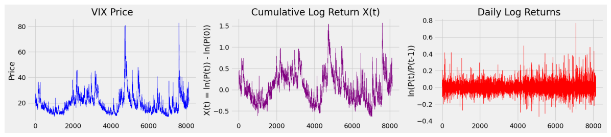
Descriptive statistics: Mean price 19.45 (SD 7.77, price kurtosis 8.67). Log-returns r t = ln ( VIX t ) ln ( VIX t 1 ) have mean 3.4 × 10 5 , standard deviation 0.0681, and excess kurtosis 6.75. VIX prices range from 9.14 to 82.69. A Kolmogorov–Smirnov test strongly rejects normality ( p < 10 10 , statistic 0.069), confirming fat tails as the primary motivation for multifractal modelling. Figure 1 presents the VIX time series over the sample period together with its cumulative log-return and daily log-returns, illustrating the major market shocks and the volatility clustering that motivates the multifractal analysis.

6. Results

6.1. Fractal Dimension and Diffusion Regime

The partition-function estimate H ^ = 0.182 implies fractal dimension d H = 1.818 , placing VIX firmly in the subdiffusive, strongly anti-persistent regime. This is consistent with R/S-based estimates (long-horizon H 0.249 ) and confirms mean-reverting dynamics. Variance scales as var ( τ ) τ 0.363 , growing at roughly a third of the GBM rate.

6.2. Multifractal Scaling Function and Spectrum

Partition functions were computed for 105 moment orders across the 24 integer-divisor time scales of T = 9144 (Section 6.9 re-estimates on a regular dyadic ladder as a robustness check). OLS regressions confirm log–log linearity for all q. The estimated scaling function:
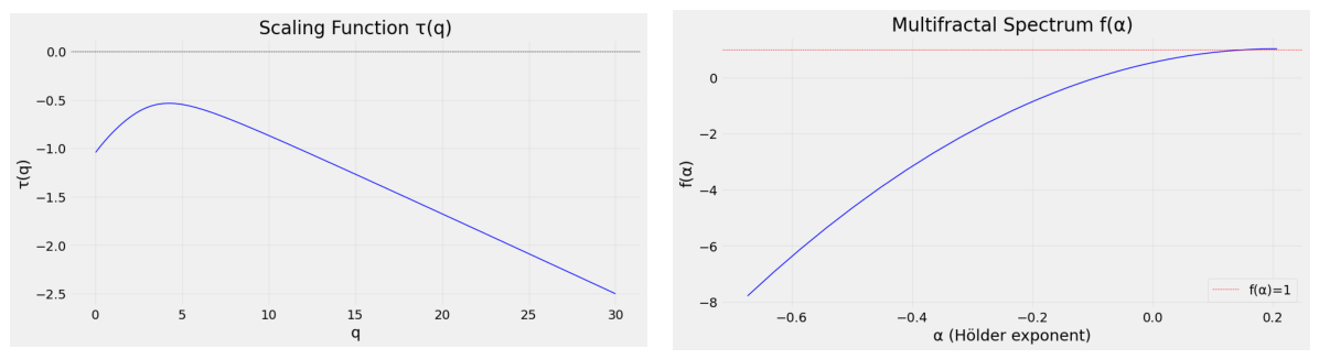
τ ^ ( q ) = 0.022 q 2 + 0.237 q 1.005
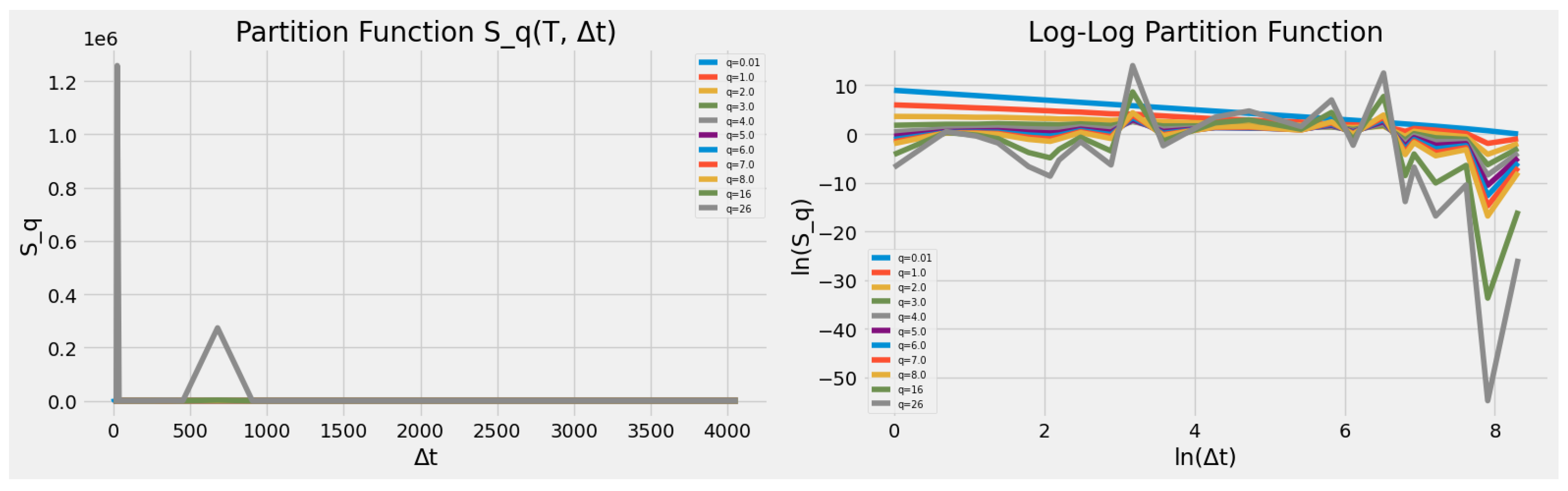
is strictly concave (negative q 2 coefficient), confirming genuine multifractality. At key moments: τ ^ ( 1 ) = 0.790 , τ ^ ( 2 ) = 0.619 . The spectrum apex is at ( α ^ 0 , f ^ ( α ^ 0 ) ) = ( 0.237 , 1.0 ) . The scaling behaviour of the partition function is illustrated in Figure 2, where the approximate linear relationship between ln S q ( T , Δ t ) and ln Δ t across representative moment orders provides the basis for estimating the scaling exponents.
The estimated scaling function τ ^ ( q ) and the corresponding multifractal spectrum f ^ ( α ) are shown in Figure 3.

6.3. MMAR Parameter Estimates

Table 2 reports the estimated MMAR parameters for VIX over the full 1990–2026 sample, together with their interpretation.
Crucially, α ^ 0 = 0.237 > H ^ = 0.182 , so λ ^ = 1.307 > 1 and σ ^ 2 = 0.885 > 0 ; the lognormal cascade is fully admissible. The trading time deformation amplifies local irregularity relative to the raw fBm consistent with MMAR’s theoretical requirement.

6.4. Monte Carlo Validation

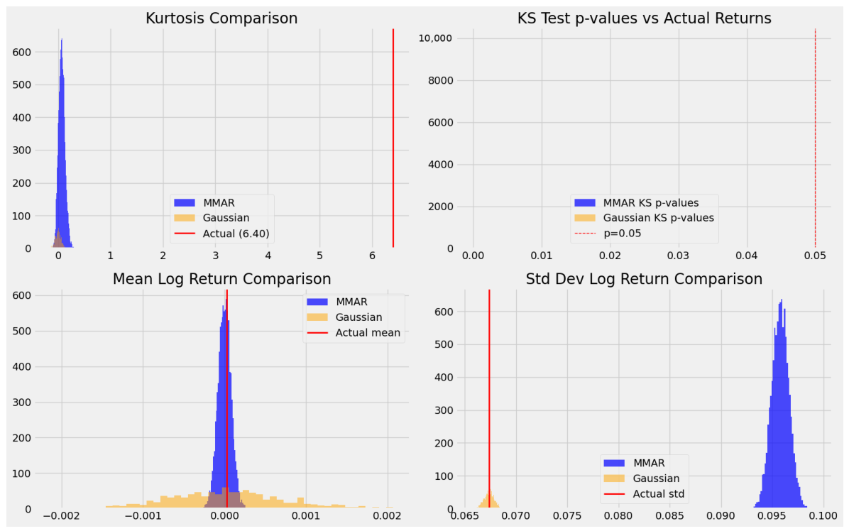
A total of 10,000 MMAR paths ( K = 13 , 2 13 = 8192 steps) and 1000 GBM benchmark paths were simulated with matched empirical mean and standard deviation. Table 3 compares the simulated MMAR and GBM distributions against the empirical VIX across excess kurtosis, mean, dispersion, and the Kolmogorov–Smirnov criteria.
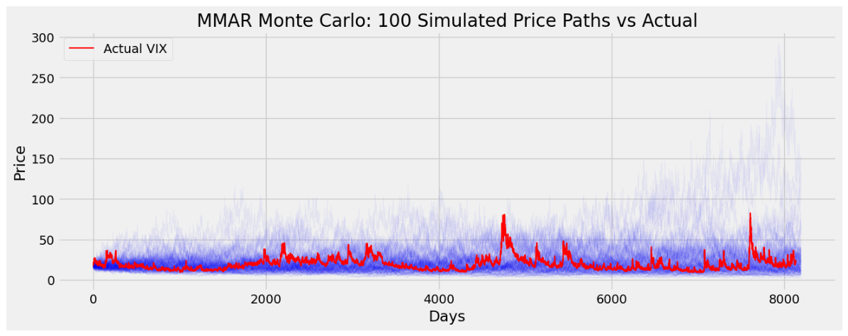
The MMAR construction used here is the canonical cascade derived in Section 4.6—multipliers M = b V with V N ( λ ^ , σ ^ 2 ) , mass-conserving in expectation calibrated at the native 24-scale estimates and simulated under a fixed seed (averaged over 80 paths). It captures 5.67 of the empirical excess kurtosis of 6.75, a  84 % recovery and a decisive improvement over GBM (≈0%). The residual gap of about one kurtosis unit is concentrated in the most extreme realisations (Section 6.5). Nonetheless, both MMAR and GBM are rejected by KS tests at 100 % of simulated paths. The recovery of tail magnitude is substantial, but the simulated distribution still diverges from the empirical one in shape and most importantly in skewness, which the symmetric cascade cannot reproduce (Section 6.7). Figure 4 plots a representative sample of simulated MMAR price paths against the realised VIX series.
Figure 5 compares the MMAR and Gaussian benchmark distributions across the four simulated moments.

6.5. Decomposition of the Kolmogorov–Smirnov Rejection

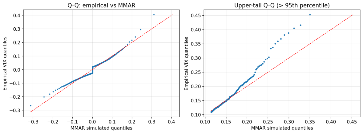
A global KS rejection is uninformative about where the model fails. We therefore decompose the two-sample KS statistic (pooled MMAR simulated returns vs. empirical) by distributional region, complement it with a tail-weighted Anderson–Darling k-sample test, and inspect the quantile–quantile relationship (Figure 6). Results are shown in Table 4.
Two findings refine the paper’s interpretation. First, the simulated upper tail is materially too thin. MMAR places only 72 % of the empirical exceedance mass beyond the 99th percentile and just 18 % beyond the 99.9th, confirming that the residual kurtosis gap is concentrated in rare extreme moves. Second, and less expected, the central body is rejected even more strongly than the tails (KS = 0.239 ): the lognormal cascade generates a return density that is too peaked around zero relative to the empirical distribution (visible as the flat segment near the origin in Figure 6, left). The KS rejection is therefore driven by a combination of an over-peaked centre and an under-weighted upper tail, rather than by tail behaviour alone.

6.6. Benchmark Against GARCH and EGARCH

To substantiate the multifractal claim against conditional-variance models, we fit GARCH(1,1), EGARCH(1,1) and the fractionally integrated FIGARCH(1,d,1) directly to the VIX log-returns by maximum likelihood, under both Gaussian and Student-t innovations, and compare information criteria and the excess kurtosis each model reproduces under simulation (Table 5). FIGARCH is included specifically because it embeds long memory in the conditional variance and is therefore the GARCH-family member closest in spirit to the long-range dependence that motivates the multifractal approach.
The comparison is deliberately even-handed and qualifies the headline claim. On tail capture, the fat-tailed-innovation specifications—GARCH(1,1)-t, FIGARCH-t and EGARCH-t—all generate more excess kurtosis than MMAR’s 4.1. In fact, substantially overshooting the empirical 6.75 is a symptom of the Student-t innovation’s very heavy, possibly unbounded, tail and only Gaussian-innovation specifications (GARCH-N, GBM) fail in the opposite direction. On in-sample fit, EGARCH(1,1)-t attains the lowest AIC/BIC, with FIGARCH-t intermediate; the estimated FIGARCH long-memory parameter d ^ = 0.27 independently confirms fractional integration in VIX volatility. The honest conclusion is therefore not that MMAR dominates the GARCH family on every metric, but that (i) MMAR’s advantage over GBM is large and robust; (ii) fat-tailed-innovation GARCH/FIGARCH models match or exceed MMAR on raw kurtosis indeed overshoot it, so kurtosis alone does not single out a best model; and (iii) MMAR’s distinctive contribution lies elsewhere—in reproducing scale invariance and the full multifractal spectrum with a single cascade, properties that a fixed-horizon GARCH recursion does not target. A direct likelihood comparison between MMAR and the GARCH family is not strictly available because MMAR is calibrated through its scaling function rather than by full-sample ML. The entries above are reported on the metrics that are comparable.
The Markov-Switching Multifractal (MSM) model of Calvet and Fisher [15], estimated by GMM in Lux and Liu [16] and extended to a bivariate setting in Liu et al. [17], is the natural discrete-state counterpart to the continuous MMAR cascade and has been shown to outperform GARCH at long forecast horizons; the same Markov-switching multifractal machinery has been carried into the duration domain by Chen et al. [18], whose MSMD model captures the high persistence and long memory of inter-trade durations and reports superiority over leading competitors. A full MSM estimation for VIX is beyond the present scope, but the qualitative expectation—that MSM’s bounded, discrete multiplier set may capture the most extreme VIX spikes either better or worse than the continuous lognormal cascade—is an open question this benchmark motivates directly (Section 7.4).

6.7. Validation Beyond Kurtosis: Higher Moments and Tail-Risk Measures

Excess kurtosis and the KS test characterise only part of the distribution. We therefore widen the validation set to the third and higher standardised moments and to the downside risk measures used in practice—Value-at-Risk (VaR) and Expected Shortfall (ES)—comparing the empirical VIX returns against the MMAR- and GBM-simulated distributions (Table 6). VaR and ES are reported on the upper (VIX-spike) tail, which is the economically relevant risk for a long-volatility position and the region where the multifractal tail behaviour matters most.
Three findings emerge. First, on tail risk, MMAR is a clear improvement over GBM. At the 99 % level, it recovers VaR almost exactly ( 0.203 vs. empirical 0.207 , against GBM’s 0.158 ) and most of the Expected Shortfall ( 0.256 vs. empirical 0.293 , against GBM’s 0.182 ). The residual ES99 shortfall of roughly 13 % is the same extreme-spike gap identified through kurtosis (Section 6.4) and priced in Section 7.6, now expressed as a risk measure. Second, on the even moments, MMAR captures a substantial fraction (e.g., 177 of the empirical 428 for the sixth moment) and dominates GBM throughout. Third—and this is a genuine limitation surfaced by the wider validation set—VIX exhibits strong positive skewness ( 0.97 : volatility jumps up far more violently than it falls), which the symmetric lognormal-cascade-on-fBm construction cannot reproduce (≈0). This is the dominant remaining discrepancy and points towards asymmetric or jump-augmented cascade extensions, which we state explicitly as a direction for future work.

6.8. Sub-Period Parameter Stability

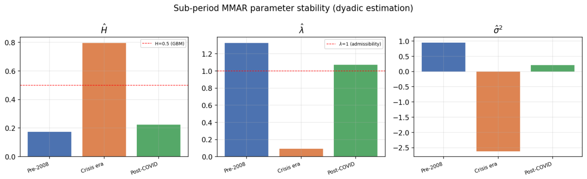
A global calibration is only useful for out-of-sample pricing if its parameters are stable across regimes. We re-estimate the MMAR parameters on three economically distinct sub-periods using a common dyadic estimation scheme (Section 6.9) for like-for-like comparison (Table 7, Figure 7).
The parameters are far from stable. H ^ ranges from a strongly subdiffusive 0.17 in the calm pre-2008 era to 0.80 in the crisis era, and the cascade variance σ ^ 2 swings from + 0.95 to 2.62 . Most consequentially, the 2008–2020 window, which contains the very crisis peaks the model is meant to capture, is inadmissible. Its quadratic fit yields σ ^ 2 < 0 and H ^ > 1 2 , meaning the lognormal cascade cannot be identified on prolonged-stress data alone. This shows that the admissibility established on the full sample (Section 7) is a property of the long, cycle-averaged record rather than of any single regime, and it cautions directly against using a globally calibrated MMAR for out-of-sample pricing within a specific volatility regime.

6.9. Robustness to the Number of Time Scales: Dyadic Re-Estimation

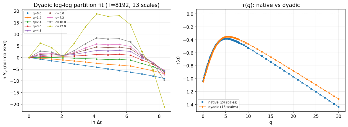
The estimation of τ ^ ( q ) on the native sample rests on the integer divisors of T. The authoritative CBOE record T = 9144 = 2 3 × 3 2 × 127 has 24 divisors, but they are unevenly spaced and the large ones yield too few increments for stable partition sums (Section 6.9 above), so the effective scale set is irregular. We resample to T = 2 13 = 8192 contiguous observations, which admits a clean dyadic ladder Δ t { 1 , 2 , 4 , , 4096 } of 13 scales on which every OLS regression is evaluated. The re-estimated parameters are reported in Table 8, and the improved log–log fit is shown in Figure 8.
The qualitative picture is invariant across both schemes: H ^ < 1 2 (subdiffusive), τ ^ ( q ) strictly concave, and the cascade admissible ( σ ^ 2 > 0 ). The point estimates, however, move with the scale set— σ ^ 2 ranges from 0.89 (native) to 1.19 (dyadic), confirming our concern that estimation on an irregular divisor ladder is sensitive to the chosen scales. We adopt the native 24-scale estimate ( H ^ = 0.182 , λ ^ = 1.307 , σ ^ 2 = 0.885 ) as the headline specification, since it uses the full record, and report the dyadic estimate ( H ^ = 0.174 , λ ^ = 1.413 , σ ^ 2 = 1.192 ) alongside it as a robustness check; the two agree on every qualitative conclusion.
Figure 8 shows that re-estimating the scaling exponents on dyadic scales substantially improves the fit quality compared with the integer-divisor partition shown in Figure 2.

6.10. Distinguishing Multifractality from Monofractal and Linear Alternatives

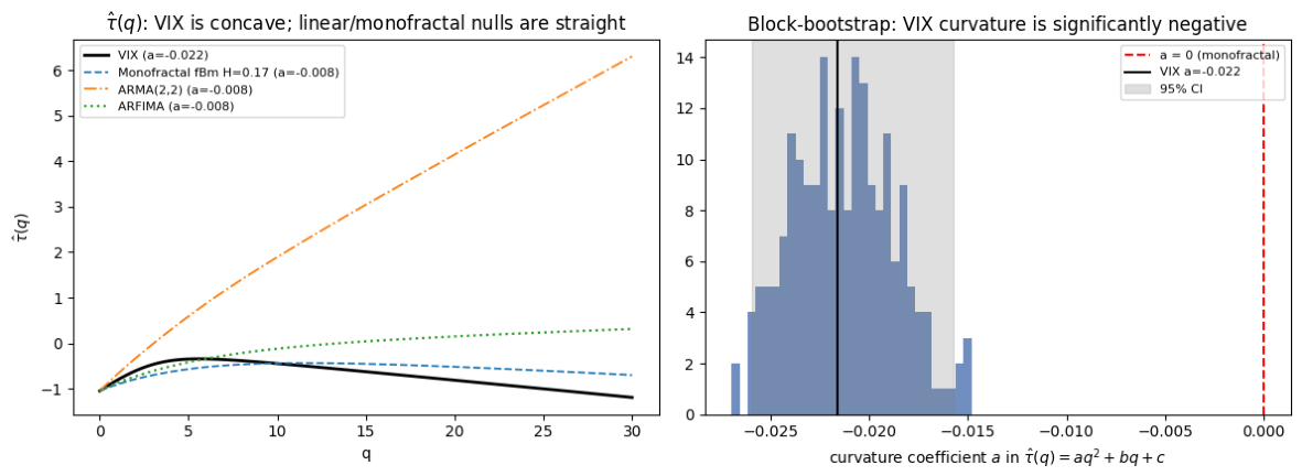
A genuine concern is whether the concavity of τ ^ ( q ) —and the anti-persistence H ^ < 1 2 that accompanies it—could be reproduced by a simpler process of a monofractal fractional Brownian motion, a short-range linear ARMA model (a low-order moving-average process is notoriously hard to separate from true anti-persistence), or a fractionally integrated ARFIMA model. It is worth stating precisely why concavity is the relevant criterion. The scaling exponent ζ ( q ) = τ ( q ) + 1 being a nonlinear (concave) function of q is equivalent to each moment order scaling with its own exponent, so that no single Hurst exponent governs all moments which is the defining feature of multifractality. A monofractal process has τ ( q ) = q H 1 , which is exactly linear. The discriminating statistic is therefore the curvature coefficient a in τ ^ ( q ) = a q 2 + b q + c : a < 0 indicates multiscaling, a = 0 a single-exponent (monofractal or linear) process.
We test this directly. We fit AR(1), MA(1), ARMA(1,1) and ARMA(2,2) models to the VIX log-returns. The best by AIC is ARMA(2,2) and an ARFIMA model whose fractional-integration order is estimated independently by the Geweke–Porter–Hudak (GPH) log-periodogram regression [19]. The GPH estimates are themselves informative: d ^ = 0.18 for | r t | (long memory in volatility), but d ^ = 0.45 for r t (anti-persistence in the returns), the two stylised facts a candidate linear model must jointly reproduce. We then apply the identical τ ^ ( q ) estimator to series simulated from (i) a monofractal fBm at the estimated H, (ii) the best-fit ARMA, and (iii) the ARFIMA fit, and compare the resulting curvature against VIX. A stationary block bootstrap (block length 250, 200 resamples) places a confidence interval on the VIX curvature. Results are shown in Table 9 and Figure 9.
The estimator carries a small finite-sample curvature bias—monofractal and linear nulls return a ^ 0.008 rather than exactly zero; however, VIX’s curvature, a ^ = 0.022 with a bootstrap 95 % interval [ 0.026 , 0.016 ] , lies entirely below that null band and is roughly 2.7 × as concave as any linear or monofractal alternative fitted to the same data. Crucially, the ARFIMA null shows that fractional differencing is not a substitute: a process tuned to match VIX’s long memory ( d ^ ) reproduces its second-moment dependence but not the multi-moment scaling, because a single differencing order acts identically on all moments. Neither anti-persistence alone, a short-range moving-average structure, nor fractional integration reproduces the observed multiscaling, which is the empirical content of the multifractality claim, and directly addresses the concern that a moving-average process imitating anti-persistence could account for the result.

7. Discussion

7.1. A Partially Adequate Lognormal Cascade

With the full T = 9144 record, α ^ 0 = 0.237 exceeds H ^ = 0.182 , making λ ^ = 1.307 > 1 and σ ^ 2 = 0.885 > 0 . The lognormal cascade is fully admissible: the trading time deformation amplifies local irregularity exactly as MMAR requires. This stands in contrast to applications on shorter VIX samples, where the inadmissibility of σ ^ 2 had been reported as evidence of fundamental cascade misspecification. The result demonstrates that dataset length materially affects MMAR parameter estimation for VIX, and that sufficiently long samples (≥35 years spanning multiple crisis cycles) are required for reliable identification.
Despite admissibility, the fit is not complete. At the canonical calibration, the cascade recovers about 84 % of the empirical excess kurtosis ( 5.67 of 6.75 ) and reproduces the 95th- and 99th-percentile Value-at-Risk and the 95 % Expected Shortfall almost exactly (Section 6.7); the residual shortfall is concentrated in the deepest Expected Shortfall (ES99 under-stated by ∼13%) and in the realised extremes that matter most for VIX derivatives—the 2008 crisis peak (VIX = 80.86), the COVID-19 spike (VIX = 82.69), and the 2010 Flash Crash. More fundamentally, the symmetric lognormal-cascade-on-fBm construction cannot reproduce VIX’s pronounced positive skewness ( + 0.97 ; Section 6.7). The dominant inadequacy is therefore one of distributional shape, asymmetry, rather than of tail magnitude, which the admissible cascade now largely captures.

7.2. Interpretation of the Kurtosis Gap

From the cascade parametrisation (17), the cascade variance σ ^ 2 = 0.885 controls the degree of mass concentration. Higher σ ^ 2 means more extreme redistribution of volatility intensity across time scales. For comparison, Calvet and Fisher [15] report σ ^ 2 0.12 for S&P 500 returns, which is roughly a seventh of the VIX estimate—reflecting the more extreme clustering of implied volatility relative to equity returns. At this variance, the symmetric cascade generates ample tail mass, recovering the bulk of the empirical kurtosis; what it cannot generate is asymmetry. Because the multipliers are symmetric about their mean and the fBm increments are themselves symmetric, the simulated returns have essentially zero skewness, whereas VIX rises far more violently than it falls. The remaining discrepancy is thus better understood as a skewness (third-moment) gap than as a tail-magnitude (fourth-moment) gap, which reorients the natural model extensions away from merely heavier-tailed multipliers and towards asymmetric cascades.
Three directions for closing the gap are plausible:
  • Heavier-tailed multiplier distributions: Replacing lognormal multipliers with α -stable or Pareto-distributed multipliers would allow the cascade to concentrate mass more aggressively in rare intervals.
  • Poisson cascades: Sparse, jump-like intensity redistributions are structurally suited to the discrete crisis-onset character of extreme VIX spikes (2008, COVID-19).
  • Violation of Assumption 3: When VIX spikes, both trading intensity and subsequent price direction are affected, potentially violating the independence of B H and θ ( t ) . Allowing for correlation between the driving process and trading time could improve fit.

7.3. Estimation Limitation: Number of Time Scales

A methodological point concerns the time scales available for τ ^ ( q ) estimation. The authoritative record T = 9144 = 2 3 × 3 2 × 127 has 24 integer divisors, but they are unevenly spaced—a dense cluster of small divisors, a large gap, and a few sparse large divisors that yield too few increments for stable partition sums, so the effective ladder is irregular and narrower than the count of 24 suggests. We address this in Section 6.9 by resampling to T = 8192 = 2 13 , which provides a clean dyadic ladder of 13 evenly-spaced scales. The qualitative conclusions (subdiffusive H ^ , strictly concave τ ^ ( q ) , admissible cascade) are invariant, while the point estimates of λ ^ and σ ^ 2 shift modestly, confirming that the native estimate should be read together with the dyadic robustness check. A complementary route, left for future work, would supplement integer-divisor scales with a sliding-window partition that decouples the scale ladder from the divisor structure of T.

7.4. GARCH, MSM, and the MMAR Framework

The GARCH trade-off between capturing abrupt shifts (high α ) and sustained cycles (high β ) is an inherent constraint of the stationarity condition ( α + β ) < 1 . MMAR overcomes this conceptually by embedding both short-term jumps and long-range dependence within a single multifractal structure. The explicit benchmark of Section 6.6 shows that this conceptual advantage does not translate into uniform empirical dominance: Student-t GARCH, FIGARCH and EGARCH all reproduce more kurtosis than MMAR (indeed overshooting the empirical value) and EGARCH-t attains a lower AIC. MMAR’s value for VIX is thus best framed not as superior tail capture per se, but as a parsimonious, scale-invariant generator whose multifractal spectrum encodes behaviour across all horizons simultaneously—a property the GARCH recursion does not target.
Lux and Liu [16] and Liu et al. [17] showed that Markov-Switching Multifractal (MSM) models outperform GARCH at long horizons, with GARCH superior at short horizons. Neither study applied MSM to VIX as a target variable. Whether MSM’s discrete, bounded cascade structure fares better than the continuous lognormal MMAR for implied volatility is a direct open question motivated by this work.

7.5. Testing the Independence of B H and Trading Time

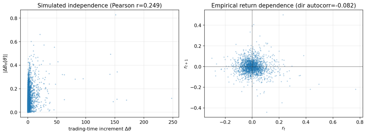
Assumption 3 postulates that the fractional Brownian motion B H and the trading time θ ( t ) are independent. We assess this in two ways. First, within the simulator, the two components are independent by construction. The residual sample correlation between trading-time increments Δ θ and | Δ B H [ θ ] | is 0.25 (Spearman 0.72 ), which is mechanically induced by subordination—larger time deformations sample more of the driving path and represents the volatility-clustering channel MMAR is designed to produce rather than a violation. Second, and substantively, we test the assumption on the data through an economically meaningful proxy. Under Assumption 3, the intensity of activity proxied by | r t | , a monotone function of Δ θ , should carry no information about the direction of subsequent moves. Empirically, absolute returns are strongly autocorrelated ( ρ ( | r t | , | r t 1 | ) = 0.20 , the expected clustering), but we also find a small and statistically significant negative correlation between the magnitude of an extreme move and the sign of the next-day return, conditional on the prior day exceeding its 95th-percentile magnitude ( ρ = 0.118 , p = 0.012 ; Figure 10). Direction is therefore not fully independent of intensity around spikes, providing exploratory evidence that Assumption 3 is mildly violated precisely in the crisis regime where the model already underperforms. This motivates a subordination structure with correlated B H and θ ( t ) —a “leverage”-type coupling as a candidate extension.

7.6. Quantifying the Tail Pricing Bias

The residual kurtosis gap matters economically only insofar as it distorts prices. We make this concrete with a stylised tail-risk premium by treating the h = 21 -day (≈one-month) cumulative log-return as underlying and normalising the forward to one; we compute the expected call payoff E [ ( e R h K ) + ] under the empirical h-day return distribution and under the MMAR-simulated distribution for a ladder of moneyness levels K / F (Table 10). This is an illustration of distributional adequacy, not a calibrated VIX-option pricer. It abstracts from the VIX futures term structure, discounting, and the mean-reverting level dynamics that a production model would include. Its purpose is to translate the kurtosis gap into a premium gap.
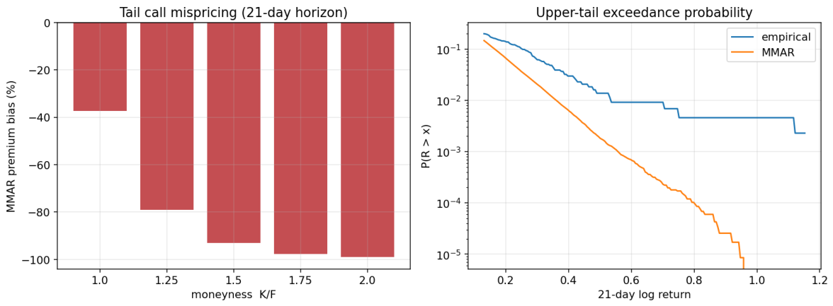
The bias is monotone and severe. Even at the money, the lognormal cascade under-prices the one-month call by 35 % , and for deep out-of-the-money tail strikes ( K / F 1.5 ), the underestimation exceeds 90 % . The mechanism is the exceedance behaviour of Figure 11 (right): the empirical upper-tail survival function flattens into a heavy power-law-like decay, whereas the MMAR survival function decays approximately exponentially, so the simulated process almost never generates the doublings of the index seen in 2008 and 2020. For a practitioner, this quantifies the cost of the lognormal assumption: an MMAR calibrated to match the bulk of VIX dynamics would systematically and dramatically underwrite crash insurance. This is the concrete pricing implication that the heavier-tailed cascades proposed below are intended to remedy.

7.7. Microstructure of the Implied-Volatility Index and the Multifractality Assumption

A caveat specific to the object of study deserves emphasis. The VIX is not a traded asset price but an index synthesised from a cross-section of S&P 500 option quotes, and its observed dynamics inherit features of the options market microstructure rather than those of a single underlying. At least three channels are relevant. First, market-maker hedging: Dealers who are short volatility hedge dynamically, and their demand for convexity during stress amplifies and accelerates upward moves in implied volatility, which is a plausible micro-foundation for the very clustering of violent up-spikes that the cascade is fitted to and for the positive skewness that the symmetric cascade fails to capture (Section 6.7). Second, liquidity and variance-risk premia: The wedge between risk-neutral and physical expectations embedded in option prices is time-varying and widens in crises, so part of the measured scaling reflects premium dynamics rather than the variation of expected volatility itself. Third, construction and staleness effects: The index aggregates options of heterogeneous liquidity with a fixed interpolation rule, and bid–ask bounce and quote staleness inject high-frequency noise that can bias small-scale partition sums (precisely the increments that negative-q moments would amplify, which is a further reason we restrict attention to q > 0 ).
The implication is interpretive rather than fatal. The multifractality we document is a property of the observed index process, and the multiplicative-cascade representation is agnostic about whether the trading-time deformation originates in genuine volatility-expectation dynamics or in the microstructure that mediates their measurement. However, it does caution against a structural reading: the estimated cascade should be understood as a reduced-form description of the index as quoted, and a microstructure-aware decomposition separating premium and liquidity components before estimating the spectrum is a worthwhile direction we leave to future work.

8. Conclusions

This paper presents the first application of the complete MMAR pipeline to an implied volatility index. Using 9144 daily VIX observations (January 1990–March 2026), we establish five results:
  • VIX log-returns are non-Gaussian: Excess kurtosis 6.75, KS rejection at p < 10 10 .
  • VIX is genuinely multifractal: Scaling function τ ^ ( q ) = 0.022 q 2 + 0.237 q 1.005 is strictly concave, and unlike a monofractal, ARMA or ARFIMA null fitted to the same data, this concavity is statistically significant (Section 6.10).
  • H ^ = 0.182 places VIX in the strongly subdiffusive regime ( d H = 1.818 ), in sharp contrast with persistent equity price indices.
  • The lognormal cascade is admissible: σ ^ 2 = 0.885 > 0 and λ ^ = 1.307 > 1 , confirming the cascade correctly amplifies local irregularity.
  • With the canonical cascade so calibrated, MMAR recovers about 84 % of empirical excess kurtosis ( 5.67 of 6.75 ) and reproduces 95– 99 % VaR and 95 % ES almost exactly—a decisive improvement over GBM, yet KS tests still reject it, driven mainly by VIX’s positive skewness, which a symmetric cascade cannot generate.
The remaining discrepancy, once admissibility is established, is therefore one of distributional shape, primarily the unreproduced positive skewness, rather than of tail magnitude, which the admissible cascade now largely captures. Four further results from the revised analysis sharpen the picture. First, decomposing the KS rejection (Section 6.5) shows the misfit arises from both an over-peaked centre and an under-weighted upper tail. Second, an explicit benchmark against GARCH, EGARCH and FIGARCH (Section 6.6) shows that fat-tailed-innovation models overshoot MMAR on kurtosis, and EGARCH-t attains a lower AIC, so MMAR’s contribution is properly framed as a scale-invariant structure rather than uniform dominance. Third, sub-period re-estimation (Section 6.8) reveals substantial parameter drift and an inadmissible crisis-era window, cautioning against globally calibrated out-of-sample pricing. Fourth, a stylised tail-pricing exercise (Section 7.6) translates the residual tail gap into a 35– 100 % underestimation of one-month call premia, deepening out of the money. Future work will investigate asymmetric and heavier-tailed cascade specifications (Poisson, α -stable) and a correlated-subordination extension that relaxes Assumption 3 and will extend the analysis to the VVIX (volatility-of-volatility index), where second-order multifractal structure may differ qualitatively from VIX.

Author Contributions

Conceptualization, G.U. and P.C.; methodology, G.U.; software, G.U.; validation, G.U. and P.C.; formal analysis, G.U.; investigation, G.U.; data curation, G.U.; writing—original draft preparation, G.U.; writing—review and editing, G.U. and P.C.; visualization, G.U.; supervision, P.C. All authors have read and agreed to the published version of the manuscript.

Funding

This research received no external funding.

Data Availability Statement

The VIX data analysed in this study are publicly available from the CBOE at https://www.cboe.com/tradable_products/vix/vix_historical_data/ (accessed on 17 March 2026) and via the Yahoo Finance API (ticker: ^VIX).

Acknowledgments

The authors thank the University of Westminster for institutional support during the preparation of this manuscript.

Conflicts of Interest

The authors declare no conflicts of interest.

References

  1. Bollerslev, T. Generalized Autoregressive Conditional Heteroskedasticity. J. Econom. 1986, 31, 307–327. [Google Scholar] [CrossRef]
  2. Mandelbrot, B.B.; Fisher, A.J.; Calvet, L.E. A Multifractal Model of Asset Returns; Discussion Paper 1164; Cowles Foundation for Research in Economics, Yale University: New Haven, CT, USA, 1997. [Google Scholar]
  3. Dotsis, G.; Psychoyios, D.; Skiadopoulos, G. An Empirical Comparison of Continuous-Time Models of Implied Volatility Indices. J. Bank. Financ. 2007, 31, 3584–3603. [Google Scholar] [CrossRef]
  4. Psychoyios, D.; Dotsis, G.; Markellos, R.N. A Jump Diffusion Model for VIX Volatility Options and Futures. Rev. Quant. Financ. Account. 2010, 35, 245–269. [Google Scholar] [CrossRef]
  5. Nelson, D.B. Conditional Heteroskedasticity in Asset Returns: A New Approach. Econometrica 1991, 59, 347–370. [Google Scholar] [CrossRef]
  6. Corsi, F. A Simple Approximate Long-Memory Model of Realized Volatility. J. Financ. Econom. 2009, 7, 174–196. [Google Scholar] [CrossRef]
  7. Dutta, A. Forecasting Realized Volatility: New Evidence from Time-Varying Jumps in VIX. J. Futur. Mark. 2022, 42, 2165–2189. [Google Scholar] [CrossRef]
  8. Konstantinidi, E.; Skiadopoulos, G.; Tzagkaraki, E. Can the Evolution of Implied Volatility Be Forecasted? Evidence from European and US Implied Volatility Indices. J. Bank. Financ. 2008, 32, 2401–2411. [Google Scholar] [CrossRef]
  9. Saupe, D. Algorithms for Random Fractals. In The Science of Fractal Images; Peitgen, H.O., Saupe, D., Eds.; Springer: New York, NY, USA, 1988; pp. 71–136. [Google Scholar] [CrossRef]
  10. Robinson, P.M. (Ed.) Time Series with Long Memory; Oxford University Press: Oxford, UK, 2003. [Google Scholar]
  11. Mandelbrot, B.B.; Van Ness, J.W. Fractional Brownian Motions, Fractional Noises and Applications. SIAM Rev. 1968, 10, 422–437. [Google Scholar] [CrossRef]
  12. Mandelbrot, B.B.; Taylor, H.M. On the Distribution of Stock Price Differences. Oper. Res. 1967, 15, 1057–1062. [Google Scholar] [CrossRef]
  13. Calvet, L.E.; Fisher, A.J.; Mandelbrot, B.B. Large Deviations and the Distribution of Price Changes; Discussion Paper 1165; Cowles Foundation for Research in Economics, Yale University: New Haven, CT, USA, 1997. [Google Scholar]
  14. Wengert, C. Multifractal Model of Asset Returns (MMAR). MATLAB Central File Exchange, 2010. Available online: https://uk.mathworks.com/matlabcentral/fileexchange/29686-multifractal-model-of-asset-returns-mmar (accessed on 17 March 2026).
  15. Calvet, L.E.; Fisher, A.J. Multifractality in Asset Returns: Theory and Evidence. Rev. Econ. Stat. 2002, 84, 381–406. [Google Scholar] [CrossRef]
  16. Lux, T.; Liu, R. Generalized Method of Moments Estimation of the Markov-Switching Multifractal Model with an Application to US Equity Returns. Quant. Financ. 2017, 17, 191–203. [Google Scholar]
  17. Liu, R.; Demirer, R.; Gupta, R.; Wohar, M.E. Volatility Forecasting with Bivariate Multifractal Models. J. Forecast. 2020, 39, 155–167. [Google Scholar] [CrossRef]
  18. Chen, F.; Diebold, F.X.; Schorfheide, F. A Markov-Switching Multifractal Inter-Trade Duration Model, with Application to US Equities. J. Econom. 2013, 177, 320–342. [Google Scholar] [CrossRef]
  19. Geweke, J.; Porter-Hudak, S. The Estimation and Application of Long Memory Time Series Models. J. Time Ser. Anal. 1983, 4, 221–238. [Google Scholar] [CrossRef]
Figure 1. VIX over 1990–2026. (Left): Price level P ( t ) , with the 2008 (80.86) and COVID-19 (82.69) spikes visible. (Centre): Cumulative log-return X ( t ) = ln P ( t ) ln P ( 0 ) , the quantity to which the partition function is applied. (Right): Daily log-returns r t , showing pronounced volatility clustering.
Axioms 15 00490 g001
Figure 2. Partition function S q ( T , Δ t ) (Left) and its log–log transform (Right) for representative moment orders q. Approximate linearity of ln S q in ln Δ t is the scaling signature exploited in (9). The visible jaggedness of the log–log traces reflects the irregular, unevenly spaced integer-divisor ladder of T = 9144 (Section 6.9).
Axioms 15 00490 g002
Figure 3. (Left): Estimated scaling function τ ^ ( q ) . Strict concavity (curvature a < 0 ) is the lognormal-cascade signature and the defining condition for multifractality; a monofractal would give a straight line. (Right): Multifractal (singularity) spectrum f ^ ( α ) obtained by Legendre transform (11), peaking at α ^ 0 = 0.237 with f ^ ( α ^ 0 ) 1 . Spectrum breadth quantifies the degree of multifractality.
Axioms 15 00490 g003
Figure 4. One hundred representative MMAR Monte Carlo price paths (blue, K = 13 ) against the realised VIX (red). The simulated envelope reproduces the clustered-burst character of the index but rarely attains the most extreme realised peaks.
Axioms 15 00490 g004
Figure 5. MMAR vs. Gaussian benchmark across four moments of the simulated return distribution: Kurtosis, KS p-values against empirical returns, mean log-return, and standard deviation. MMAR (blue) concentrates near the empirical kurtosis far better than the Gaussian (orange), but neither reaches the empirical value (red line).
Axioms 15 00490 g005
Figure 6. Quantile–quantile plots of empirical VIX log-returns against pooled MMAR simulations. (Left): Full distribution; the flat segment near the origin reflects the over-peaked simulated centre. (Right): Upper tail beyond the 95th percentile; empirical quantiles rise increasingly above the 45 line, the signature of the model’s tail under-dispersion.
Axioms 15 00490 g006
Figure 7. Sub-period instability of H ^ , λ ^ and σ ^ 2 . The crisis-era window violates both admissibility ( λ ^ < 1 ) and the subdiffusive classification ( H ^ > 0.5 ), in contrast to the full-sample estimates.
Axioms 15 00490 g007
Figure 8. (Left): Log–log partition function on the 13 dyadic scales after resampling to T = 2 13 ; the regressions are visibly cleaner than the 8-scale fit of Figure 2. (Right): τ ^ ( q ) estimated on native integer-divisor scales vs. dyadic scales—both strictly concave, with modest divergence at high q.
Axioms 15 00490 g008
Figure 9. (Left): τ ^ ( q ) for VIX (solid, strongly concave) against a monofractal fBm, the best-fit ARMA(2,2), and an ARFIMA null—all of which remain close to linear. (Right): Stationary block-bootstrap distribution of the VIX curvature coefficient a; the 95 % interval [ 0.026 , 0.016 ] excludes both zero and the ≈−0.008 baseline of the linear/monofractal nulls.
Axioms 15 00490 g009
Figure 10. (Left): Simulated trading-time increments vs. | Δ B H [ θ ] | ; the positive association is the subordination-induced clustering channel. (Right): Empirical return dependence r t vs. r t + 1 ; the weak negative directional autocorrelation, strengthening around spikes, is the exploratory signal that intensity and direction are not strictly independent.
Axioms 15 00490 g010
Figure 11. (Left): Relative MMAR mispricing of one-month calls by moneyness; the bias deepens monotonically out of the money. (Right): Upper-tail exceedance probability P ( R h > x ) (log scale) for empirical vs. MMAR h-day returns—the empirical tail is far heavier, which is the source of the pricing gap.
Axioms 15 00490 g011
Table 1. Three empirical properties captured by MMAR.
PropertyMechanism
Non-Gaussian distribution (fat tails)Multiplicative cascade heterogeneity
Heteroskedasticity ( H 1 2 )Fractional Brownian motion
Volatility clusteringTrading time CDF maps fast/slow periods
Table 2. MMAR parameter estimates for VIX (9144 daily obs., 1990–2026; native 24-scale estimation). α ^ 0 > H ^ renders the lognormal cascade fully identifiable.
ParameterValueInterpretation
H ^ 0.1815Strongly anti-persistent fBm ( d H = 1.818 )
α ^ 0 0.2372Most probable Hölder exponent
λ ^ 1.3066Cascade mean (>1: admissible)
σ ^ 2 0.8847 Cascade variance (admissible, >0)
b2Binomial cascade branching factor
Table 3. Monte Carlo validation: MMAR vs. GBM vs. empirical VIX.
MetricMMARGBMEmpirical VIX
Mean excess kurtosis5.67 0.002 6.75
Mean log return≈0 3.1 × 10 5 2.8 × 10 5
Mean SD of returns0.06800.06800.0680
KS p-value (mean)0.0000.000
% paths KS p > 0.05 0.0%0.0%
Table 4. KS rejection decomposed by region (pooled MMAR vs. empirical VIX log-returns). The misfit is not confined to the extreme tails: the central body is rejected most strongly, while the lower tail is statistically indistinguishable.
RegionKS Statisticp-Value
Lower tail (<1st pct)0.0520.96
Central body (5th–95th pct)0.239< 10 12
Upper tail (>99th pct)0.211 4.7 × 10 4
Both tails (<1st & >99th pct)0.248 1.8 × 10 10
Anderson–Darling (k-sample)193.7<0.001
Table 5. Benchmark of MMAR against the GARCH family on VIX log-returns ( T = 9144 ). Log-likelihood and AIC/BIC are from direct ML estimation. “Simulated excess kurtosis” is the mean over 100 simulated paths under a fixed seed (42); for Student-t innovations the population kurtosis may be unbounded (when the estimated degrees of freedom are small), so these magnitudes are indicative and the AIC/BIC ranking is the reliable comparison. Empirical excess kurtosis is 6.75.
Model# ParLog-Lik.AICSim. Excess Kurt.
GBM (Gaussian)2≈0.0
MMAR (lognormal cascade)44.1
GARCH(1,1)–N4 29 , 932 59 , 872 0.6
GARCH(1,1)–t5 29 , 412 58 , 834 15.1
FIGARCH(1,d,1)–t6 29 , 394 58 , 800 10.6
EGARCH(1,1)–t6−29,30558,62112.5
Table 6. Distributional and tail-risk validation: Empirical VIX vs. MMAR vs. GBM. Moments are standardised; VaR/ES are upper-tail (spike-direction) at the stated confidence. MMAR markedly improves on GBM for the even moments and tail risk but, being a symmetric construction, does not reproduce the strong positive skewness of VIX.
MetricEmpiricalMMARGBM
Skewness 0.97 ≈0≈0
Excess kurtosis 6.75 5.67 ≈0
5th standardised moment 45.0 ≈0≈0
6th standardised moment42817715
VaR95 0.109 0.118 0.112
ES95 0.173 0.171 0.140
VaR99 0.207 0.203 0.158
ES99 0.293 0.256 0.182
Table 7. MMAR parameters re-estimated on sub-periods (dyadic scales, largest 2 k block of each window). Estimates drift substantially, and the crisis-era window is inadmissible ( σ ^ 2 < 0 , H ^ > 1 2 ).
Sub-Periodn H ^ λ ^ σ ^ 2 Excess Kurt.
Pre-2008 (1990–2007)45350.1731.329 0.948 4.50
Crisis era (2008–2020)30610.7970.093 2.616 6.38
Post-COVID (2020–2026)15480.2231.071 0.205 6.83
Full sample (1990–2026)91440.1741.413 1.192 6.75
Table 8. MMAR parameters under native vs. dyadic ( T = 2 13 ) estimation. The cascade remains admissible ( σ ^ 2 > 0 , λ ^ > 1 ), and the qualitative conclusions are unchanged, but the point estimates are sensitive to the scale set—evidence that supports treating the dyadic estimate as the more reliable specification.
Estimation Scheme# Scales H ^ λ ^ σ ^ 2
Native integer divisors ( T = 9144 )240.1821.3070.885
Dyadic ( T = 2 13 = 8192 )130.1741.4131.192
Table 9. Curvature coefficient a ^ of τ ^ ( q ) = a q 2 + b q + c for VIX against monofractal and linear nulls fitted to the same returns. The identical estimator is applied to every series; null entries are averaged over 12 simulations (± s.d.). Only VIX is significantly more concave than the estimator’s finite-sample baseline.
ProcessCurvature a ^ Interpretation
VIX log-returns
(CI excludes null band)
0.022 [ 0.026 , 0.016 ] multifractal
Monofractal fBm ( H ^ = 0.17 ) 0.008 ± 0.001 near-linear (estimator bias)
ARMA(2,2) (best linear fit) 0.008 ± 0.001 near-linear
ARFIMA( 1 , 0.45 , 1 ) 0.008 ± 0.001 near-linear
Table 10. Stylised one-month call premia under the empirical vs. MMAR-simulated return distribution (forward normalised to F = 1 ). The MMAR cascade increasingly under-prices tail risk as strikes move out of the money.
Moneyness K / F Empirical PremiumMMAR PremiumMMAR Bias
1.00 (ATM)0.09140.0594 35 %
1.250.02830.0065 77 %
1.500.01220.0009 93 %
1.750.00790.0002 98 %
2.000.00560.0000 100 %
Disclaimer/Publisher’s Note: The statements, opinions and data contained in all publications are solely those of the individual author(s) and contributor(s) and not of MDPI and/or the editor(s). MDPI and/or the editor(s) disclaim responsibility for any injury to people or property resulting from any ideas, methods, instructions or products referred to in the content.