Nonparametric Analysis of Functional Time Series Data Using Least Absolute Relative Error Regression

Abstract

In this paper, we introduce a novel kernel-based estimator for the regression operator of a scalar response variable $\mathcal{R}$ given a functional covariate $\mathcal{F}$ taking values in a semi-metric space. The estimator is constructed through the minimization of the least absolute relative error (LARE) criterion, which provides an invariant scale and more balanced measure of predictive performance than conventional squared error methods. By focusing on relative deviations, the LARE approach effectively reduces the influence of extreme response values and enhances robustness in the presence of heteroscedasticity. From a theoretical point of view, we investigate the asymptotic behavior of the proposed estimator under strong mixing conditions for functional time series data. We show that, despite the temporal dependence structure, the estimator remains consistent and achieves convergence rates comparable to those obtained under independence. In the computational part, we show that the proposed method is computationally efficient and straightforward to implement. Its empirical performance is evaluated through simulation studies conducted under different dependence scenarios. In addition, the applicability of the method is illustrated through the analysis of a real data set.

1. Introduction

Investigating the relationship between a functional predictor and a scalar response variable is a common issue in functional data analysis. This relationship is most often studied through regression models, often estimated via the least squares criterion. However, this classical approach can be influenced by scale variability and atypical observations, which may affect its stability and accuracy. In this paper, we propose an alternative smoothing framework based on the least absolute relative error (LARE). By working with relative deviations rather than least square error, the LARE criterion yields a more robust estimation procedure and generally leads to improved predictive performance compared with standard regression methods.

The general setting of this paper concerns nonparametric prediction for functional data. It constitutes an active research area that has gained substantial progress in recent years. The pioneering contribution in this direction was made by [1], who established the almost complete pointwise consistency of kernel-based regression estimators under the assumption of independent and identically distributed (i.i.d.) observations. Next, ref. [2] derived convergence results in the ($L^p$) norm, while [3] established the moment integrability of the same estimator in the same independence framework. The asymptotic normality of the kernel estimator under strong mixing dependence conditions was proven in [4]. Ref. [5] considers the k-nearest neighbor (kNN) estimators for a nonparametric functional regression model under negatively associated dependence. They proved the almost complete consistency. More recently, ref. [6] addresses a more general setting for functional covariates by assuming that the regressors take values in Riemannian manifolds. Under a strong mixing dependence framework, explicit expressions for the bias and variance of the proposed estimator are established. As an alternative to the classical kernel approaches, more recent studies have explored (M)-estimation techniques as well as local linear smoothing methods. A comprehensive overview of nonparametric functional prediction can be found in [7,8], which provide detailed surveys of these developments.

In contrast to these classical approaches, we focus on relative error (RE) regression, where the loss function is defined through relative deviations rather than conventional scoring functions. Such a formulation is particularly attractive in applications where scale invariance plays an important role. Despite its practical appeal, the development of nonparametric RE regression remains relatively limited, as most existing contributions have been devoted to parametric or semiparametric settings. One of the earliest contributions in this direction is given by [8], who investigated estimation procedures based on the relative squared error loss. From the applied studies, RE regression has been successfully employed in a variety of fields, including medical studies [9] and financial modeling [10]. Furthermore, ref. [11] examined RE-based estimation within multiplicative regression models, while ref. [12] extended the methodology to the nonparametric framework and established consistency and convergence results for local linear estimators under relative error loss.

In recent years, increasing attention has been given to RE regression in the presence of dependent data structures. For instance, ref. [13] studied RE-based estimation for spatial time series models. The first nonparametric functional RE regression framework was introduced by [14], who established strong consistency and derived the asymptotic distribution of the associated estimator. This result was extended in [15], where a kernel-based estimator was developed for truncated and incomplete functional data. Additional recent developments and methodological advances in this area can be found in [16,17].

While all the aforementioned studies estimate the regression operator using either the least squares (LS) or least squares relative error (LSRE) loss function, the present work adopts the absolute relative error loss within a kernel local weighting framework to construct a robust estimator for nonparametric functional regression. The resulting local absolute relative error (LARE) approach extends the classical LSRE methodology developed in [15,16] by providing enhanced robustness and improved estimation accuracy. These features are particularly important in functional time series settings, where the data are often contaminated by noise and characterized by high-frequency fluctuations. In such situations, extreme observations and local irregularities occur frequently and may substantially affect the quality of estimation. Consequently, the proposed estimator yields more stable and reliable inference for the underlying functional relationship. The robustness of the proposed LARE framework makes it especially suitable for high-frequency functional data and supports its applicability in a broad range of fields, including economics, finance, signal processing, and environmental sciences. The present contribution addresses both theoretical and practical aspects of the problem. From a theoretical perspective, we show that the nonparametric analysis of the LARE regression model is considerably more challenging than that of the LSRE framework. In particular, unlike the LSRE estimator, which admits an explicit representation in terms of ratios involving the first inverse conditional moment functionals, the LARE estimator does not possess a closed-form expression. As a consequence, its asymptotic properties cannot be derived through direct analytical arguments and instead require the development of a refined Bahadur-type representation.

Despite these technical difficulties, we establish the almost complete convergence of the proposed estimator and derive its rate of convergence under mild and standard assumptions commonly used in nonparametric functional regression. In particular, the assumptions accommodate both the functional nature of the covariates and the strong mixing dependence structure of the underlying functional time series. Such strong mixing frameworks provide a realistic setting for many modern applications in which temporal dependence plays a fundamental role, thereby making robust predictive procedures essential for reliable inference and forecasting in the presence of dependence and data contamination. The obtained results extend recent findings of [18] from the independent framework to the dependent functional time series setting. Finally, the practical relevance of the proposed methodology is illustrated through extensive simulation studies and real-data applications, both of which demonstrate the robustness and strong empirical performance of the proposed estimator.

The remainder of this paper is organized as follows. Section 2 introduces the functional time series frame and the proposed estimation methodology. Section 3 is devoted to the underlying assumptions and the establishment of the main asymptotic results. In Section 4, we discuss the applicability of the estimator in the functional prediction. Section 5 presents a comprehensive empirical assessment of the proposed estimator through simulation experiments and real data applications. Finally, Section 7 concludes the paper with some final remarks and perspectives for future research. The technical proofs are collected in Appendix A.

2. Nonparametric Functional Data Analysis

2.1. Data

The principal contribution of this work is the development of a more general framework that relaxes the conventional independence assumption, which is rarely satisfied in real-world applications. Even when the underlying dependence is weak, neglecting such structures can result in biased estimates and potentially invalid statistical inference. In this context, modelling functional time series data provides a more realistic and theoretically sound alternative, as it explicitly take into account the temporal dependence. Consequently, the proposed approach offers a more meaningful and reliable framework than methods based on independent observations. It is worth noting that functional time series (FTS) have attracted considerable attention in the functional statistics literature. Comprehensive treatments of both theoretical developments and practical applications can be found in the monographs by [19,20,21,22].

To fix ideas, we begin by recalling the definition of the strong mixing property. For this purpose, we introduce the following notation. Let $A_i^k$ denote the $\sigma$-algebra generated by the collection $\{{\mathcal{X}}_j:i\le j\le k\}$. The strong mixing coefficient, originally introduced by [23], is defined as follows; see also [24] for a comprehensive treatment.

Definition 1.

Let $X=\{{\mathcal{X}}_{i}i=1,2,\dots \}$ be a strictly stationary sequence of random variables. For any positive integer n, define

$$\begin{array}{c}\hfill \alpha \left(n\right)=\underset{k\in {\mathbb{N}}^{\ast }}{sup}sup\left\{\left|\mathbb{P}(\mathcal{A}\cap \mathcal{B})-\mathbb{P}\left(\mathcal{A}\right)\mathbb{P}\left(\mathcal{B}\right)\right|:\mathcal{A}\in A_1^k,\mathcal{B}\in A_{k+n}^{\infty }\right\}.\end{array}$$

The sequence X is said to be α-mixing (or strongly mixing) if $\alpha \left(n\right)\to 0$ as $n\to \infty$.

In this study, our analysis is based on data drawn from a sequence $X={\left\{({\mathcal{F}}_i,{\mathcal{R}}_i)\right\}}_{i\ge 1}$ of strong functional time series observations, assumed to be identically distributed as the pair $(\mathcal{F},\mathcal{R})$. Specifically, the random pair $(\mathcal{F},\mathcal{R})$ is assumed to be valued in the product space $\Im \times \mathbb{R}$, where ℑ represents a functional space equipped with a suitable semi-metric D.

2.2. Nonparametric Model

As stated in the Introduction, the main aim of this work is to analyze the relationship between a functional explanatory variable $\mathcal{F}$ and a scalar response variable $\mathcal{R}$. For this aim, we fix a point $F\in \mathrm{I}\mathrm{F}$ and consider a neighborhood ${\mathcal{V}}_F$ of F in the functional space $\mathrm{I}\mathrm{F}$. Often, the dependence between $\mathcal{F}$ and $\mathcal{R}$ was described using a least squares regression framework, defined by

$$\begin{array}{c}\hfill NR\left(F\right)=arg\underset{r}{min}\mathbb{E}\left[{\left(\mathcal{R}-r\right)}^2|\mathcal{F}=F\right].\end{array}$$

It is clear that the main advantage of this loss function is its analytical simplicity, as it allows us to derive a explicit expression of the predictor. Indeed, by taking the derivative of the criterion with respect to s, we obtain

$$NR\left(F\right)=\mathbb{E}\left[\mathcal{R}\mid \mathcal{F}=F\right].$$

(1)

Despite these advantages, standard regression methods have certain limitations. In particular, they are often sensitive to outliers, may perform poorly under model misspecification, and can be unstable in the presence of multicollinearity or high-dimensional data structures. To remedy this drawback, we consider the least absolute relative error (LARE) criterion, which yields a more robust and equilibrating treatment allowing us to reduce the influence of extreme observations. Specifically, the LARE regression is defined as

$$\begin{array}{c}\hfill RE\left(F\right)=arg\underset{r}{min}\mathbb{E}\left[\left|{\displaystyle \frac{\mathcal{R}-r}{\mathcal{R}}}\right||\mathcal{F}=F\right].\end{array}$$

(2)

In contrast to the quadratic loss in (1), this formulation is based on an absolute loss function, which improves robustness by penalizing deviations in a linear and more uniform manner. Consequently, the LARE criterion leads to a more stable and dependable evaluation of predictive performance, particularly when the data exhibit heavy tails or contain outlying observations.

For the estimation step, we use the strong functional time series observations $X={\left\{({\mathcal{F}}_i,{\mathcal{R}}_i)\right\}}_{i\ge 1}$ to construct a kernel-type estimator of $RE\left(F\right)$, defined as follows:

$$\widehat{RE}\left(F\right)=arg\underset{r}{min}{\displaystyle \frac{{\sum }_{i=1}^n\mathbf{Q}\left(f^{-1}D(F,{\mathcal{F}}_i)\right)\left|\frac{{\mathcal{R}}_i-r}{{\mathcal{R}}_i}\right|}{{\sum }_{i=1}^n\mathbf{Q}\left(f^{-1}D(F,{\mathcal{F}}_i)\right)}},$$

(3)

where $\mathbf{Q}$ is a kernel function and $f:=f_n$ is a sequence of positive real numbers tending to zero as $n\to \infty$.

The algorithm for computing this estimator is described below.

1.

Input functional sample: $X={\left\{({\mathcal{F}}_i,{\mathcal{R}}_i)\right\}}_{i=1}^n$, target curve F, kernel $\mathbf{Q}(·)$, bandwidth $f_n>0$.

2.

Compute functional distances: For each observation ${\mathcal{F}}_i$, compute the semi-metric (or distance)

$$D(F,{\mathcal{F}}_i),i=1,\dots ,n,$$

which measures the proximity between the target function F and each sample curve ${\mathcal{F}}_i$.

3.

Construct kernel weights: Transform the distances into normalized kernel weights using the bandwidth $f_n$:

$$w_i\left(F\right)=\mathbf{Q}\left({\displaystyle \frac{D(F,{\mathcal{F}}_i)}{f_n}}\right),i=1,\dots ,n.$$

These weights assign larger importance to observations whose functional predictors are closer to F.

4.

Define and minimize the weighted LARE criterion: For any candidate value r, compute the weighted loss function:

$$L_n(r;F)={\displaystyle \frac{{\sum }_{i=1}^n{w}_i\left(F\right)\left|\frac{{\mathcal{R}}_i-r}{{\mathcal{R}}_i}\right|}{{\sum }_{i=1}^n{w}_i\left(F\right)}}.$$

Obtain the estimator by solving the one-dimensional optimization problem:

$$\widehat{RE}\left(F\right)=arg\underset{r}{min}{L}_n(r;F).$$

In practice, this step can be implemented using a grid search or a convex optimization routine.

5.

Output the estimator: Return the minimizer $\widehat{RE}\left(F\right)$ as the estimated relative error regression function at F.

We point out that, in this contribution, we assume the uniqueness of the parameter $RF\left(F\right)$, whereas the uniqueness of the estimator is not necessarily required. Thus, $\widehat{RE}\left(F\right)$ denotes any solution of (3). Recall that the primary aim of the theoretical part of this paper is to investigate the asymptotic behaviour of the estimator $\widehat{RE}\left(F\right)$ of $RE\left(F\right)$, in the setting of functional time series case. To the best of our knowledge, this work provides the first construction and theoretical analysis of such an estimator within this general framework, including the multivariate case as a particular situation. Although the finite-dimensional setting can be viewed as a special case of the functional framework developed here, the infinite-dimensional context is especially relevant due to its increased mathematical complexity.

3. Main Asymptotic Result

Now, to state the almost complete convergence, we introduce generic strictly positive constants denoted by C or $C^{\prime }$. We also define

$${\mathbf{Q}}_i=\mathbf{Q}\left(f^{-1}D(F,{\mathcal{F}}_i)\right),i=1,\dots ,n.$$

The closed ball of radius f centered at F is given by

$$B(F,f)=\left\{\mathcal{F}\in \mathrm{I}\mathrm{F}:D(\mathcal{F},F)<f\right\},$$

and we define

$$U_1(r,F)=\mathbb{E}\left[{\left|\mathcal{R}\right|}^{-1}{\mathbf{1}}_{\{\mathcal{R}\le r\}}\mid T=F\right],U_2(r,F)=\mathbb{E}\left[{\left|\mathcal{R}\right|}^{-1}{\mathbf{1}}_{\{\mathcal{R}\ge r\}}\mid T=F\right].$$

We now state the following assumptions:

(RE1)

The small-ball probability satisfies

$$\mathbb{P}(T\in B(F,f))=:{\mathcal{P}}_F\left(f\right)>0,\forall f>0,$$

such that

$$lim{\mathbf{Q}}_{f\to 0}{\mathcal{P}}_F\left(f\right)=0.$$

(RE2)

For any $F_1,F_2\in {\mathcal{V}}_F$, the functions $U_{\gamma }$ are continuously differentiable with respect to r and satisfy

$$|U_{\gamma }(r,F_1)-U_{\gamma }(r,F_2)|\le C{d}^{b_{\gamma }}(F_1,F_2),b_{\gamma }>0,\gamma =1,2.$$

(RE3)

The response variable admits bounded inverse moments: for all $p\ge 2$,

$$\mathbb{E}\left[\right|\mathcal{R}{|}^{-p}\mid T=F]\le C(p,F)<\infty \mathrm{almost}\mathrm{surely}.$$

(RE4)

The sequence ${({\mathcal{F}}_i,{\mathcal{R}}_i)}_{i\in \mathrm{I}\mathrm{N}}$ satisfies: $\exists a>0,\exists c>0:\forall n\in \mathrm{I}\mathrm{N},\alpha \left(n\right)\le c{n}^{-a}$ and

$$\left\{\begin{array}{c}\forall i\ne j,\mathrm{I}\mathrm{E}\left[{\mathcal{R}}_i{\mathcal{R}}_j|{\mathcal{F}}_i,{\mathcal{F}}_j\right]\le C<\infty ,a.s.\hfill \\ \mathrm{I}\mathrm{P}\left(({\mathcal{F}}_i,{\mathcal{F}}_j)\in B(x,f)\times B(x,f)\right)={\mathcal{Q}}_F\left(f\right)>0;\hfill \end{array}\right.$$

(RE5)

The kernel function $\mathbf{Q}$ is measurable, supported on $(0,1)$, and uniformly bounded, i.e.,

$$0<C_2\le \mathbf{Q}(·)\le C_3<\infty .$$

(RE6)

There exists $\eta >0$, such that

$$C{n}^{{\displaystyle \frac{2(2-a)}{(a+1)}}+\eta }\le {\mathsf{\Phi }}_F\left(f\right)\le n^{{\displaystyle \frac{2a}{(2-a)p}}},$$

where ${\mathsf{\Phi }}_F\left(f\right)=max({\mathcal{P}}_F^2\left(f\right),{\mathcal{Q}}_F\left(f\right))$ and $a>max\left(2+1/2b_2,p/2b_2,{\displaystyle \frac{4p+1+\sqrt{24p+1}}{p-1}}\right).$

Discussion of the Assumptions

In general, these assumptions are mild and standard in the literature on functional time series analysis. The theoretical framework for nonparametric functional data analysis is essentially built upon two main components. The first, (RE1), concerns the small-ball probability function, which characterizes the concentration properties of the probability measure induced by the functional covariate. This assumption is fundamental, as it controls the stochastic fluctuations of the estimator and plays a pivotal role in the variance component of the convergence rate. The second component, (RE2), specifies the regularity of the nonparametric regression function. It is a classical smoothness assumption in functional nonparametric statistics and has been widely adopted in related works. This condition is mainly used to control the bias term in the asymptotic expansion. Assumption (RE3) is a well-known moment condition in regression analysis and is commonly employed to establish almost sure (or almost complete) consistency; see, for example, [1]. It is worth noting that (RE3) replaces the finite-variance condition typically used to ensure convergence in probability. Since almost complete convergence is a stronger form of convergence, it requires more restrictive moment assumptions. This reflects the standard trade-off between generality and strength: sharper asymptotic results generally come at the cost of stronger conditions.

Overall, the set of assumptions in this work is designed to capture three structural aspects of the model. The functional nature of the data is addressed through the concentration condition, the nonparametric structure is characterized via a Hölder-type regularity assumption, and the dependence structure is controlled by (RE4), which accounts for both global dependence across observations and local dependence within the functional trajectories. The remaining assumptions, (RE5)–(RE6), are mainly technical in nature; they are introduced to facilitate the proofs and to derive the convergence rate of the proposed estimator.

Theorem 1.

Given assumptions (RE1)–(RE6), we obtain

$$|\widehat{RE}\left(F\right)-RE\left(F\right)\left)\right|=O\left(f_n^{b_1}\right)+O\left(f_n^{b_2}\right)O\left(\sqrt{{\displaystyle \frac{{\mathsf{\Phi }}_F^{1/2}\left(f\right)logn}{n{\mathcal{P}}_F^2\left(f\right)}}}\right),a.co..$$

(4)

4. Application to Prediction in Continuous Time Process

Clearly, a particular important case of functional data is when observations are generated by a continuous-time stochastic process. In this setting, the proposed methodology can be effectively employed to predict a future real-valued feature of the process by incorporating information from its entire past trajectory in a continuous manner. Indeed, let $P_t$ denote a continuous time process observed n the interval $(0,b)$, and our goal is to predict its unobserved value at time b using an the LARE approach. To this purpose, we define N functional observations ${\left({\mathcal{F}}_i\right)}_{i=1,\dots ,N}$ by

$$\forall t\in [0,b),{\mathcal{F}}_i\left(t\right)=P_{\left(\right(i-1)b+t)/N}.$$

The associated scalar responses are defined as

$${\mathcal{R}}_i=P_{\left(ib\right)/N}.$$

Consequently, the kernel-based estimator of the LARE regression $\widehat{RE}\left({\mathcal{F}}_N\right)$ is constructed from the sample ${({\mathcal{F}}_i,{\mathcal{R}}_i)}_{i=1,\dots ,N-1}$. The asymptotic properties of this estimator are summarized in the following corollary.

Corollary 1.

Under the conditions of Theorem 1, and for sufficiently large N, we obtain

$$\widehat{RE}\left({\mathcal{F}}_N\right)-RE\left({\mathcal{F}}_N\right)\to 0\mathrm{a}.\mathrm{co}.$$

5. Computational Aspects

A Simulated Data-Driven Model

The purpose of this section is to emphasize the importance of LARE regression as a robust predictive tool. Recall that LARE regression provides a flexible, nonparametric approach to prediction, allowing to identify the complex and potentially nonlinear relationships that may be overlooked by standard regression models. Despite these advantages, the LARE model remains relatively not fully explored compared with conventional regression techniques. In many applied fields, researchers and practitioners consider the standard regression as a primary analytical tool for modeling and prediction. While widely used, standard regression often depends on restrictive requirements, namely, sensitivity to outliers or heteroscedasticity, which can limit its effectiveness in complex settings. In contrast, LARE regression offers a more robust and adaptable framework, particularly in situations characterized by asymmetry, heterogeneity, or heavy-tailed behavior. Therefore, LARE regression constitutes a powerful alternative to standard regression, providing enhanced predictive performance and greater flexibility. This illustration is designed to address three primary objectives, which are the simplicity of implementation, the impact of correlation on predictive performance and the identification of the main characteristics of the models. For these aims, we apply the algorithm of Section 4 on the dynamic of a real time series, which is generated by GARCH model, $\mathrm{GARCH}(1,1)$. It is well known that this class of processes satisfies the strong mixing assumption (see [25]), which provides a suitable theoretical foundation for the developments presented in this contribution. Formally, in this illustration, we generate a GARCH process $P_t$ as follows:

$$\left\{\begin{array}{cc}{P}_t=\mu +{ϵ}_t,\hfill & \mathrm{where}{ϵ}_t={\sigma }_t{Z}_t,\\ {\sigma }_t^2=w+\alpha {ϵ}_{t-1}^2+\beta {\sigma }_{t-1}^2,\hfill & \hfill \end{array}\right.$$

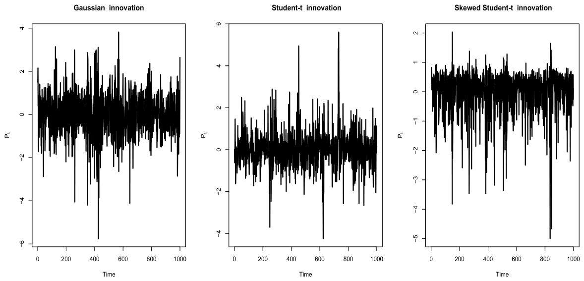
where the parameters $\omega$, $\alpha$, and $\beta$ satisfy the conditions $\omega >0$ and $\alpha +\beta <1$, ensuring the stationarity of the process. In order to covers different cases we simulate three distributions of the innovations $Z_t$ that are Gaussian, Student-t distribution and Skewed Student-t distribution. Such cases explore characteristics sch the heavy-tailed distribution as well as the symmetry or asymmetry properties. The different generated GARCH process using the routine function ugarchpath of the R-package rugarch for R version 4.4.3. The trajectories of the simulated process are displayed in Figure 1.

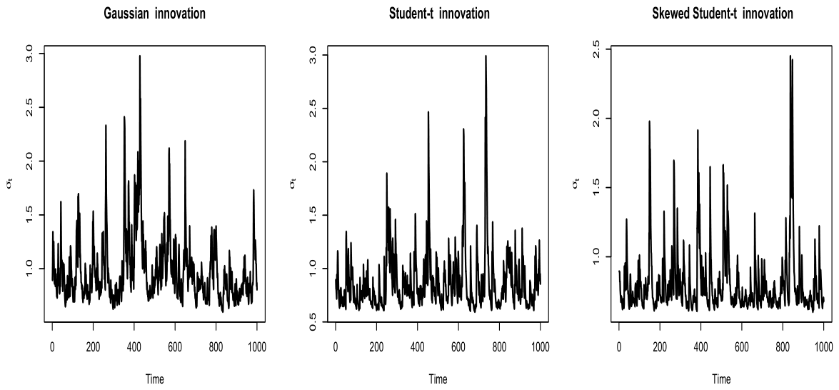
The conditional volatility for the three cases are plotted in Figure 2.

Now, in order to highlight the relevance of the nonparametric functional approach, we compare the estimator $\widehat{RE}$ with the standard regression defined by

$$\widetilde{RE}={\displaystyle \frac{{\sum }_{i=1}^n\mathbf{Q}\left(f^{-1}D(F,{\mathcal{F}}_i)\right){\mathcal{R}}_i}{{\sum }_{i=1}^n\mathbf{Q}\left(f^{-1}D(F,{\mathcal{F}}_i)\right)}}.$$

We point out that, this simulation study is conducted using a sample of 1000 observations of the pair $({\mathcal{R}}_i=P_{\left(ib\right)/N},{\mathcal{F}}_i=P_{s\in \left(\right(ib)/N,((i-1)b)/N)})$, which is divided into two subsets: the first 800 observations are used for in-sample analysis, while the remaining 200 observations are reserved for out-of-sample evaluation. Regarding the choice of the parameters involved in estimator $\widehat{RE}$ and $\widetilde{RE}$, we employ a quadratic kernel defined on $(0,1)$, along with a PCA-based metric, which is particularly suitable for handling discontinuous functional data. The optimal bandwidth is selected locally via a cross-validation procedure as follows

$$f_{\mathrm{opt}}\left(F\right)=arg\underset{f\in H_n\left(F\right)}{min}{\displaystyle \sum _{i=1}^n}\left|{\mathcal{R}}_i-{\widehat{RE}}^{-I}\left({\mathcal{F}}_i\right)\right|,$$

where $H_n\left(F\right)$ denotes the set of positive real values $f_F$ such that the ball centered at F with radius $f_F$ contains exactly $l\in \{5,10,15,\dots ,n/2\}$ nearest neighbors of F. This bandwidth selection strategy is standard in nonparametric functional statistics; see [1] for a comprehensive discussion. Furthermore, to evaluate the feasibility of the LARE regression, as well as the effect of correlation, we compare its performance with that of standard nonparametric $\widetilde{RE}$ approaches using different values $w,\alpha ,b,\beta$. Varying these parameters allows us to quantify the effect of correlation on the performance of the two estimators $\widehat{RE}$ and $\widetilde{RE}$. The mean absolute error (MAE) is used to assess the performance of both estimators.

$$MAE={\displaystyle \frac{1}{200}}\sum _{j \mathrm{in} \mathrm{the} \mathrm{testing} \mathrm{sample}}\left|{\mathcal{R}}_j-Pred\left({\mathcal{F}}_i\right)\right|$$

where $Pred$ means either $\widehat{RE}$ or $\widetilde{RE}$. The MAEs are reported in

Table 1. MAE results under different scenarios.

The Z’s Distribution	The Lag b	The Parameters $(\mathit{w},\mathit{\alpha },\mathit{\beta })$	$\widetilde{\mathit{R}\mathit{E}}$	$\widehat{\mathit{R}\mathit{E}}$
N (0,1)	5	$(0.1,0.2,0.7)$	0.024	0.032
		$(0.1,0.05,0.2)$	0.014	0.028
		$(0.2,0.05,0.2)$	0.018	0.025
		$(0.1,0.05,0.8)$	0.027	0.034
		$(0.1,0.5,0.2)$	0.025	0.033
		$(0.2,0.5,0.8)$	0.042	0.038
	15	$(0.1,0.2,0.7)$	0.028	0.035
		$(0.1,0.05,0.2)$	0.019	0.032
		$(0.2,0.05,0.2)$	0.023	0.025
		$(0.1,0.05,0.8)$	0.027	0.038
		$(0.1,0.5,0.2)$	0.029	0.038
		$(0.2,0.5,0.8)$	0.052	0.044
	30	$(0.1,0.2,0.7)$	0.033	0.038
		$(0.1,0.05,0.2)$	0.024	0.036
		$(0.2,0.05,0.2)$	0.028	0.029
		$(0.1,0.05,0.8)$	0.031	0.040
		$(0.1,0.5,0.2)$	0.037	0.046
		$(0.2,0.5,0.8)$	0.058	0.053
STD (shape = 0.4)	5	$(0.1,0.2,0.7)$	0.047	0.036
		$(0.1,0.05,0.2)$	0.041	0.023
		$(0.2,0.05,0.2)$	0.049	0.028
		$(0.1,0.05,0.8)$	0.052	0.037
		$(0.1,0.5,0.2)$	0.068	0.041
		$(0.2,0.5,0.8)$	0.086	0.030
	15	$(0.1,0.2,0.7)$	0.095	0.039
		$(0.1,0.05,0.2)$	0.061	0.037
		$(0.2,0.05,0.2)$	0.075	0.041
		$(0.1,0.05,0.8)$	0.122	0.042
		$(0.1,0.5,0.2)$	0.127	0.041
		$(0.2,0.5,0.8)$	0.182	0.052
	30	$(0.1,0.2,0.7)$	0.121	0.041
		$(0.1,0.05,0.2)$	0.123	0.045
		$(0.2,0.05,0.2)$	0.157	0.052
		$(0.1,0.05,0.8)$	0.194	0.054
		$(0.1,0.5,0.2)$	0.207	0.061
		$(0.2,0.5,0.8)$	0.256	0.072
SSTD (shape = 0.4, skew = 0.2)	5	$(0.1,0.2,0.7)$	0.089	0.042
		$(0.1,0.05,0.2)$	0.062	0.031
		$(0.2,0.05,0.2)$	0.155	0.039
		$(0.1,0.05,0.8)$	0.179	0.042
		$(0.1,0.5,0.2)$	0.207	0.046
		$(0.2,0.5,0.8)$	0.286	0.051
	15	$(0.1,0.2,0.7)$	0.398	0.054
		$(0.1,0.05,0.2)$	0.471	0.061
		$(0.2,0.05,0.2)$	0.494	0.065
		$(0.1,0.05,0.8)$	0.538	0.071
		$(0.1,0.5,0.2)$	0.587	0.079
		$(0.2,0.5,0.8)$	0.622	0.052
	30	$(0.1,0.2,0.7)$	0.657	0.062
		$(0.1,0.05,0.2)$	0.695	0.071
		$(0.2,0.05,0.2)$	0.729	0.078
		$(0.1,0.05,0.8)$	0.784	0.074
		$(0.1,0.5,0.2)$	0.827	0.084
		$(0.2,0.5,0.8)$	0.956	0.087

.

The results of this table indicate that the nonparametric functional LARE regression estimator achieves higher accuracy compared with the standard nonparametric approach. The effect of correlation on the estimation performance is important, in the sense that the MAE values increase under highly volatile settings, particularly when $\alpha +\beta$ is close to 1. However, it is clear that the LARE improves performance under heavy-tailed or skewed contamination, but it may lose efficiency under Gaussian/light-tailed settings. Overall, the main strength of the nonparametric functional LARE estimator is reflected in its flexibility, ease of implementation, and reduced sensitivity to small deviations induced by the dependence structure.

In the second part of this illustration, we investigate the robustness of the proposed estimator $\widehat{RE}$. Of course, robustness may be evaluated through several well-established criteria, including the influence function, gross-error sensitivity, breakdown point, local shift sensitivity, and bias–variance behavior under contamination, among others (see [26] for a comprehensive review). Although some of these concepts are not straightforward to generalize to functional settings, they all share the same goal of measuring the stability of an estimator and its sensitivity to different deviation in the appropriate situation. For this study, we consider the standard data (corresponds to an innovation distributed by the Standard Gaussian distribution, the lag = 30 and $(w=0.1,\alpha =0.2,\beta =0.7)$. Now, we assess the robustness of the proposed method through a contamination stress test. This approach is designed to examine how the estimator behaves when the observed data are perturbed by introducing controlled levels of contamination. In particular, the stress test provides a practical framework for evaluating the sensitivity and stability of the estimator under progressively increasing contamination proportions. Specifically, we investigate the estimator’s robustness by varying the contamination level and measuring its performance under each scenario. The following algorithm describes the detailed procedure used in this part.

Step 1

Define large scale C

Step 2

For given percentage $m\%$ we create a contaminated sample ${\mathcal{X}}_C$ by multiplying $m\%$ response values ${\mathcal{R}}_i$ by C

Step 3

Split the sample ${\mathcal{X}}_C$ into part 75% of the learning sample and 25% for the testing sample

Step 4

Compute ${\widehat{\theta }}_{m,C}=either$$\widehat{RE}$ or $\widetilde{RE}$ for the testing sample using the learning sample of ${\mathcal{X}}_C$

Step 5

Calculate $MAE$ for both estimators using the testing sample

Table 2. MAE values under different contamination levels.

n	m%	C	$\widetilde{\mathit{R}\mathit{E}}$	$\widehat{\mathit{R}\mathit{E}}$
200	10%	5	0.032	0.095
200	15%	5	0.043	0.758
200	20%	5	0.048	0.945
200	10%	10	0.063	1.789
200	15%	10	0.072	2.172
200	20%	10	0.081	2.089
300	10%	5	0.029	0.089
300	15%	5	0.038	0.142
300	20%	5	0.042	0.437
300	10%	10	0.059	0.782
300	15%	10	0.069	1.863
300	20%	10	0.072	1.967
500	10%	5	0.026	0. 086
500	15%	5	0.026	0.119
500	20%	5	0.039	0.231
500	10%	10	0.054	0.564
500	15%	10	0.067	1.557
500	20%	10	0.070	1.742

reports the MAE for various values of C, m and n.

As expected, the results confirm the superior robustness of $\widehat{RE}$ compared with $\widetilde{RE}$. In particular, the MAE associated with $\widehat{RE}$ exhibits low variability across different contamination levels, indicating that the LARE regression estimator is both stable and highly robust. Specifically, its MAE ranges from $0.026$ to $0.081$, reflecting only mild sensitivity to increasing contamination. By contrast, the estimator $\widetilde{RE}$ shows substantially higher variability, with MAE values ranging from $0.086$ to $2.089$, which indicates a considerable degradation in performance under contamination. These results clearly highlight the robustness advantage of the proposed LARE approach through its consistently low error variability.

6. Real Data Application

This section introduces a new predictive approach for financial time series using the studied LARE regression, with particular attention to its feasibility in volatility forecasting and option pricing. We perform a comparative analysis of several regression-based predictors designed to enhance the empirical prediction of asset returns, which play a central role in derivative valuation. This framework offers considerable flexibility for exploring the complex and the irregular dynamics that characterize financial markets. Therefore, the robustness of the studied model is particularly important in option pricing, where an accurate representation of tail behavior and volatility dynamics is crucial for reliable valuation.

For the empirical analysis, we consider closed-prices (of frame of 5 min) of Bitcoin Cryptocurrency. The data was retrieved from the Stooq database (available in https://stooq.com/db/h/, accessed on 18 March 2026) and it covers the period from 31 October 2025 to 15 March 2026. The resulting time series displays clear evidence of volatility clustering, rapid fluctuations, and strong temporal dependence features that present substantial challenges for financial models. These properties highlight the practical relevance of robust and nonparametric approaches for both volatility forecasting and derivative pricing. In practice, financial analysis is generally performed using log-returns rather than raw prices. Accordingly, we define the log-return process as

$$P\left(t\right):=100\left(log\left(\mathcal{Z}\left(t\right)\right)-log\left(\mathcal{Z}(t-1)\right)\right),$$

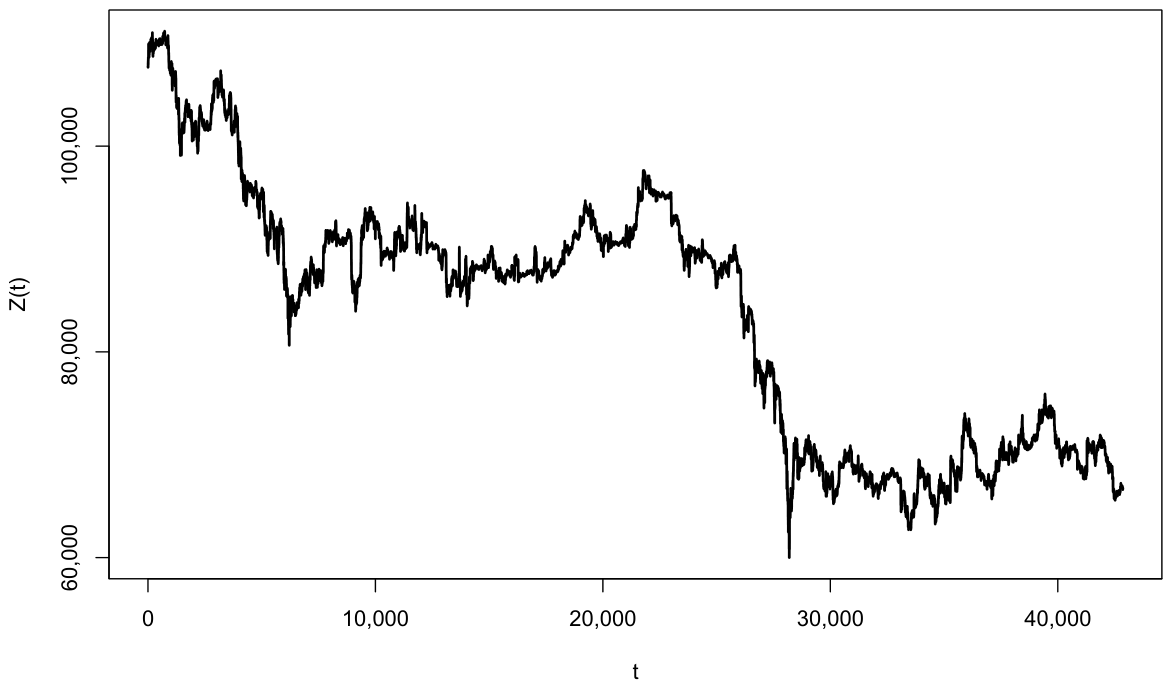
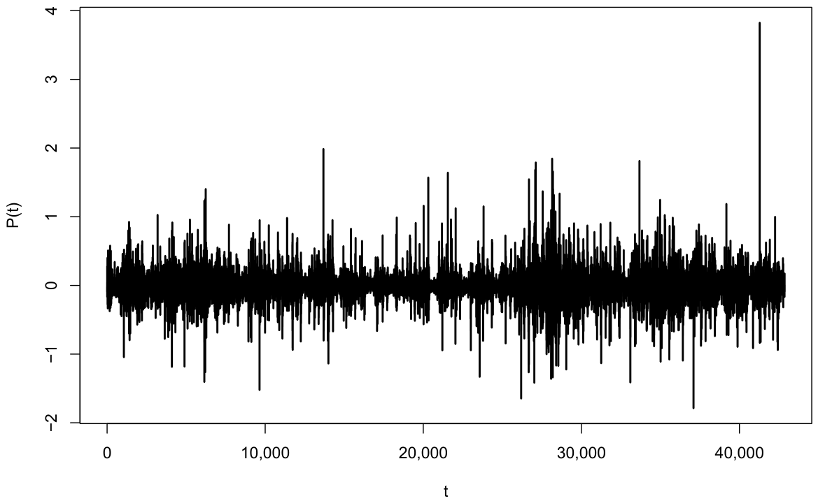
where $\mathcal{Z}\left(t\right)$ represents the asset price at time t. The resulting series $\left(Z\right(t),P(t\left)\right)$ are illustrated in Figure 3 and Figure 4.

It is evident that the series $P\left(t\right)$ is affected by certain outliers. To quantify these observations, we employ the median absolute deviation (MAD) function. Using this procedure, a total of 11.71% observations are considered as outliers in the dataset. Our main objective is to forecast one-day ahead, which motivates the examination of the stochastic process ${\left\{P\left(s\right)\right\}}_{s\in [0,T)}$. It is well established that financial return series typically display zero mean with substantial volatility. These two features highlight the nature dynamic of the asset returns. According to the algorithm of the functional time series data developed in Section 4, we construct a functional sample by cutting the series $\left\{P\right(s\left)\right\}$ into $N=135$ curves, each representing one day of observations.

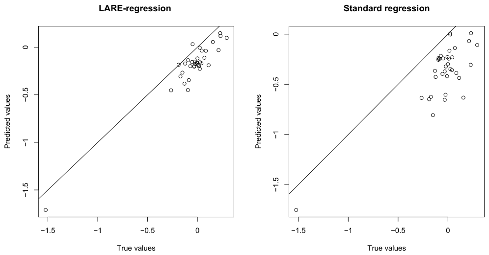
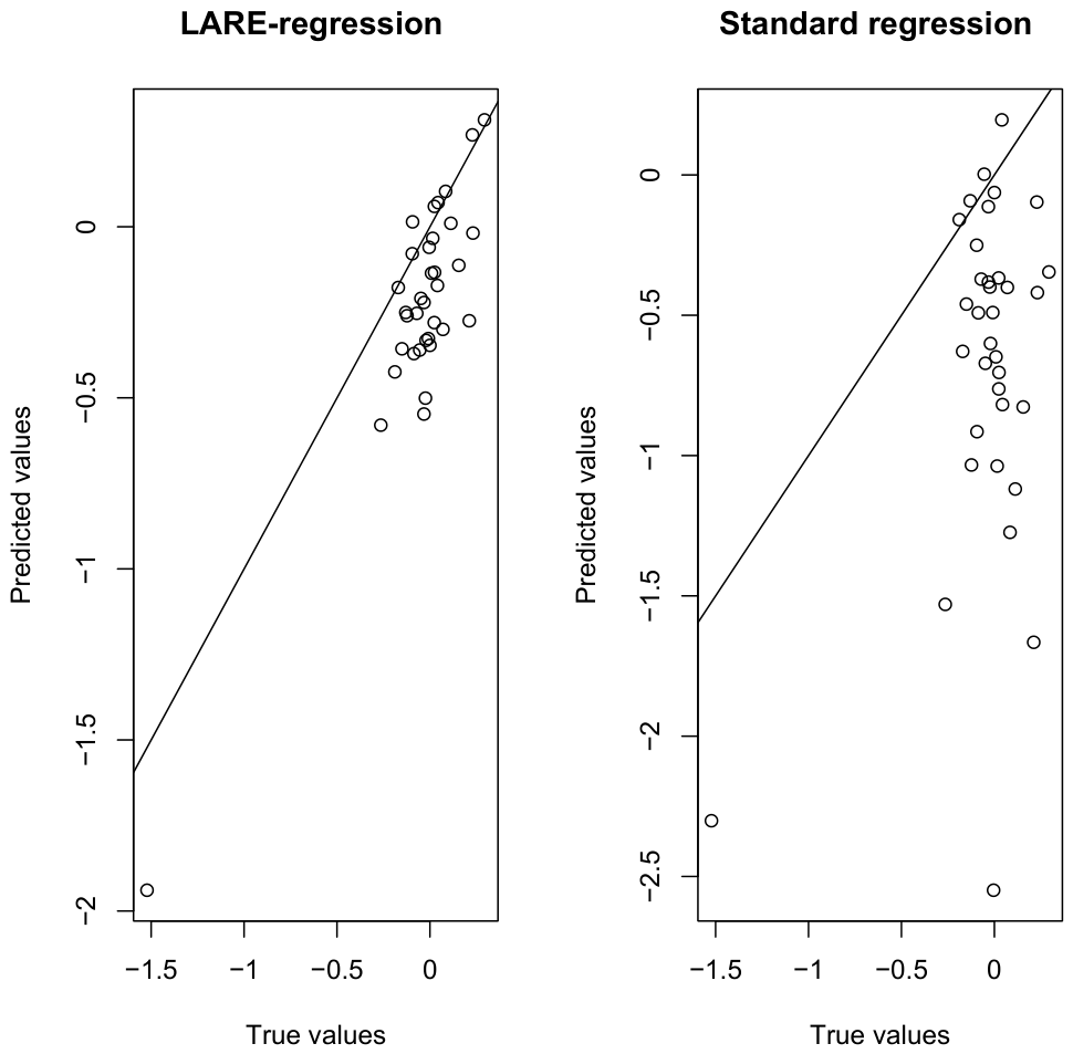
Although our primary goal is to predict the total day return, we further assess the performance of the proposed method by comparing it with a classical regression estimator based on the conditional expectation, denoted by $\widetilde{RE}$. To illustrate the added value of the LARE-regression approach, the prediction analysis is carried out under two scenarios: in the first, the analysis is performed on the original data $P\left(T\right)$ containing outliers, while in the second, outliers are removed. Keeping the same strategy of the previous section to select the principal parameters including the smoothing parameter, the metric D and the same kernel $\mathbf{Q}$ we obtain the following results (see Figure 5 and Figure 6 ). In these figures we plot predicted values against the true values in both case (initial data and clean data).

The empirical results demonstrate that the LARE-regression estimator, $\widehat{RE}$, delivers more accurate predictions than the conventional least-squares estimator, $\overline{RE}$. This superiority is confirmed through the comparison of the mean absolute error (MAE) obtained under the two estimation procedures across both data configurations. For the original dataset, where outliers are retained, the MAE associated with the LARE-regression estimator is only $0.082$, whereas the classical least-squares approach yields a substantially larger error of $0.37$. A similar statement is observed after the removal of outliers: the MAE under the LARE framework remains low at $0.09$, while the least-squares estimator still exhibits a markedly higher error of $1.03$.

This conclusion clearly underline the robustness of the LARE-regression approach. In particular, the estimator maintains stable and reliable predictive performance even in the presence of extreme observations and irregular fluctuations, conditions that commonly arise in financial time series. This robustness makes the proposed functional methodology especially well suited for modeling and forecasting data characterized by high volatility and heavy-tailed behavior.

7. Conclusions and Prospects

The present work introduces a robust framework for functional regression estimation based on the least absolute relative error (LARE) loss function. We develop a novel estimator and establish its asymptotic properties, demonstrating its strong consistency. The functional structure is characterized using the small-ball probability function, which explores the topological properties of the probability measure associated with the functional explanatory variable. Moreover, the use of the LARE criterion substantially enhances the robustness of the regression model. The asymptotic theory is developed under general assumptions, explicitly accommodating strong mixing functional time series. This guarantees that the results hold for a wide range of dependent functional data and continuous-time processes.

Empirical analyses illustrate the ease of implementing the proposed estimator. We demonstrate that it can be applied straightforwardly, with several established techniques available for selecting the smoothing parameter. Computational results further highlight the superiority of the LARE-based functional regression in terms of both robustness and predictive accuracy relative to alternative approaches.

Despite these advantages, some limitations of the proposed nonparametric LARE regression approach should be noted. In particular, the estimator may exhibit sensitivity when the response variable takes values close to zero. In such situations, the relative error term can become excessively large or unstable, which may affect the estimation procedure and generate numerical instability. Therefore, although the relative error framework provides improved robustness in many practical settings, special attention is required when analyzing data that contain small response values.

This contribution also opens several avenues for future research. A natural extension would be to develop a local linear variant of this robust modal regression estimator, as local linear modeling is known to improve convergence rates and reduce boundary bias. Establishing the asymptotic normality of the proposed estimator is another important open problem, essential for constructing confidence intervals and conducting hypothesis tests. Additional directions include exploring linear or partially linear formulations of the regression model. A particularly challenging but impactful extension would be adapting these methods to more complex data structures, such as censored data or ergodic functional time series. Of course addressing these challenges require novel mathematical tools and theoretical developments beyond the scope of the present study.

References

1. Ferraty, F.; Vieu, P. The functional nonparametric model and application to spectrometric data. Comput. Stat. 2002, 17, 545–564. [Google Scholar] [CrossRef] [Scilit]
2. Dabo-Niang, S.; Rhomari, N. Estimation non paramétrique de la régression avec variable explicative dans un espace métrique. Comptes Rendus Math. 2003, 336, 75–80. [Google Scholar] [CrossRef] [Scilit]
3. Delsol, L. Régression non-paramétrique fonctionnelle: Expressions asymptotiques des moments. In Annales de l’ISUP; LSTA: Paris, France, 2007; Volume 51, pp. 43–67. [Google Scholar]
4. Masry, E. Nonparametric regression estimation for dependent functional data: Asymptotic normality. Stoch. Process. Their Appl. 2005, 115, 155–177. [Google Scholar] [CrossRef] [Scilit]
5. Hu, X.; Wang, J.; Wang, L.; Yu, K. K-nearest neighbor estimation of functional nonparametric regression model under NA samples. Axioms 2022, 11, 102. [Google Scholar] [CrossRef] [Scilit]
6. Wiem, N.; Salah, K.; Françoise, Y.A. Nonparametric regression on Riemannian manifolds under an α-mixing process. Commun. Stat.–Theory Methods 2026, 1–16. [Google Scholar] [CrossRef] [Scilit]
7. Barrientos-Marin, J.; Ferraty, F.; Vieu, P. Locally modelled regression and functional data. J. Nonparametr. Stat. 2010, 22, 617–632. [Google Scholar] [CrossRef] [Scilit]
8. Narula, S.C.; Wellington, J.F. Prediction, linear regression and the minimum sum of relative errors. Technometrics 1977, 19, 185–190. [Google Scholar] [CrossRef]
9. Chatfield, C. The joys of consulting. Significance 2007, 4, 33–36. [Google Scholar] [CrossRef] [Scilit]
10. Chen, K.; Guo, S.; Lin, Y.; Ying, Z. Least absolute relative error estimation. J. Am. Stat. Assoc. 2010, 105, 1104–1112. [Google Scholar] [CrossRef] [Scilit] [PubMed]
11. Yang, Y.; Ye, F. General relative error criterion and M-estimation. Front. Math. China 2013, 8, 695–715. [Google Scholar] [CrossRef] [Scilit]
12. Jones, M.C.; Park, H.; Shin, K.I.; Vines, S.K.; Jeong, S.O. Relative error prediction via kernel regression smoothers. J. Stat. Plan. Inference 2008, 138, 2887–2898. [Google Scholar] [CrossRef] [Scilit]
13. Attouch, M.; Laksaci, A.; Messabihi, N. Nonparametric relative error regression for spatial random variables. Stat. Pap. 2017, 58, 987–1008. [Google Scholar] [CrossRef] [Scilit]
14. Demongeot, J.; Hamie, A.; Laksaci, A.; Rachdi, M. Relative-error prediction in nonparametric functional statistics: Theory and practice. J. Multivar. Anal. 2016, 146, 261–268. [Google Scholar] [CrossRef] [Scilit]
15. Altendji, B.; Demongeot, J.; Laksaci, A.; Rachdi, M. Functional data analysis: Estimation of the relative error in functional regression under random left-truncation model. J. Nonparametr. Stat. 2018, 30, 472–490. [Google Scholar] [CrossRef] [Scilit]
16. Benzamouche, S.; Ould Saïd, E.; Sadki, O. Nonparametric estimation of the relative error regression for twice censored and dependent data. Commun. Stat.–Theory Methods 2025, 54, 1492–1525. [Google Scholar] [CrossRef] [Scilit]
17. Xia, X.; Ming, H.; Li, J. Relative error model average for multiplicative models. Stat. Comput. 2026, 36, 18. [Google Scholar] [CrossRef] [Scilit]
18. Laksaci, A.; Almanjahie, I.M.; Rachdi, M. Nonparametric Functional Least Absolute Relative Error Regression: Application to Econophysics. Mathematics 2026, 14, 268. [Google Scholar] [CrossRef] [Scilit]
19. Wang, J.L.; Chiou, J.M.; Müller, H.G. Functional data analysis. Annu. Rev. Stat. Its Appl. 2016, 3, 257–295. [Google Scholar] [CrossRef] [Scilit]
20. Bosq, D. Linear Processes in Function Spaces: Theory and Applications; Springer Science & Business Media: Berlin/Heidelberg, Germany, 2000; Volume 149. [Google Scholar] [CrossRef] [Scilit]
21. Horváth, L.; Kokoszka, P.; Reeder, R. Estimation of the mean of functional time series and a two-sample problem. J. R. Stat. Soc. Ser. B (Stat. Methodol.) 2013, 75, 103–122. [Google Scholar] [CrossRef] [Scilit]
22. Amato, U.; Antoniadis, A.; De Feis, I.; Gijbels, I. Functional time series forecasting: A systematic review. Stat. Pap. 2025, 66, 21. [Google Scholar] [CrossRef] [Scilit]
23. Rosenblatt, M. A central limit theorem and a strong mixing condition. Proc. Natl. Acad. Sci. USA 1956, 42, 43–47. [Google Scholar] [CrossRef] [Scilit] [PubMed]
24. Bradley, R.C.; Jurek, Z.J. The strong mixing and the selfdecomposability properties. Stat. Probab. Lett. 2014, 84, 67–71. [Google Scholar] [CrossRef] [Scilit]
25. Francq, C.; Zakoian, J.M. Mixing properties of a general class of GARCH(1,1) models without moment assumptions on the observed process. Econom. Theory 2006, 22, 815–834. [Google Scholar] [CrossRef] [Scilit]
26. Maronna, R.A.; Martin, R.D.; Yohai, V.J.; Salibian-Barrera, M. Robust Statistics: Theory and Methods (with R); John Wiley & Sons: Hoboken, NJ, USA, 2019. [Google Scholar] [CrossRef] [Scilit]
27. Hallin, M.; Lu, Z.; Yu, K. Local linear spatial quantile regression. Bernoulli 2009, 15, 659–686. [Google Scholar] [CrossRef] [Scilit]
28. Ruppert, D.; Carroll, R.J. Trimmed least square estimation in the linear model. J. Am. Stat. Assoc. 1980, 75, 828–838. [Google Scholar] [CrossRef]
Figure 1. The GARCH process, μ = 0 , w = 0.1 , α = 0.2 , β = 0.7 .
Axioms 15 00397 g001
Figure 2. The σ t process, μ = 0 , w = 0.1 , α = 0.2 , β = 0.7 .
Axioms 15 00397 g002
Figure 3. The Z ( t ) -process.
Axioms 15 00397 g003
Figure 4. The P ( t ) -process.
Axioms 15 00397 g004
Figure 5. The cleaned data (data without outliers).
Axioms 15 00397 g005
Figure 6. The initial data (data with outliers).
Axioms 15 00397 g006