A Solitonic Approach of General Relativistic Spacetimes with Applications

Abstract

In this article, some remarkable results on general relativistic spacetimes with non-constant scalar curvature $\tau$, admitting almost Ricci-Bourguignon solitons and gradient almost Ricci-Bourguignon solitons, have been established. Finally, a non-trivial example of a general relativistic spacetime is constructed by using partial differential equations to validate some of our findings.

1. Introduction

A pseudo-Riemannian manifold $\mathcal{M}$ (dim. $\mathcal{M}=n$) endowed with a metric of signature $(n-1,1)$, is called a Lorentzian n-manifold [1]. In general relativity and cosmology, spacetime is modeled as a connected four-dimensional Lorentzian manifold. A general relativistic spacetime (GRS) refers to a Lorentzian 4-manifold that satisfies Einstein’s field equations. General relativity, introduced by Einstein, is the modern geometric theory of gravitation. It generalizes special relativity, refines Newton’s law of universal gravitation, and provied a mathematical to describe the gravitational phenomena in modern physics. The physical and geometric properties of the spacetimes have been investigated by many authors, such as, see [2,3,4,5,6].

Perfect fluid spacetimes play a key role to study Einstein’s field equations (EFEs). If the Ricci tensor $S(\ne 0)$ of a GRS fulfills the relation

$$\begin{array}{c}\hfill S={\sigma }_{1}g+{\sigma }_2\omega \otimes \omega ,\end{array}$$

(1)

here ${\sigma }_1,{\sigma }_2\in C^{\infty }\left(\mathcal{M}\right)$, the set of smooth functions on $\mathcal{M}$; then the spacetime is called a perfect fluid spacetime (PFS). Here, the 1-form $\omega$ is associated with the unit timelike vector field (UTVF) $\zeta$, satisfying

$$g(\zeta ,\zeta )=\omega \left(\zeta \right)=-1,g(·,\zeta )=\omega (·).$$

In case, when ${\sigma }_2=0$, (1) reduces to the Einstein condition, and hence the PFS leads to Einstein spacetime. Noting that a Robertson-Walker spacetime is a PFS [7]. The geometric and physical properties of PFSs has been extensively studied by several authors in [8,9,10,11,12]. Throughout this manuscript, $({\mathcal{M}}^4,\zeta )$ denotes a four-dimensional GRS admitting a special UTVF $\zeta$ satisfying $\nabla \zeta =I+\omega \otimes \zeta$, where ∇ is the Levi-Civita connection

The Ricci flow, introduced by Hamilton [13], is defined on an $(\mathcal{M},g)$ by the evolution equation

$${\displaystyle \frac{\partial g}{\partial t}}=-2S,g\left(0\right)=g_0.$$

The metric g on $\mathcal{M}$ satisfying the relation

$${\pounds }_{\mathcal{F}}g+2S=2\vartheta g,$$

here $\vartheta \in \mathbb{R}$ (the set of real numbers) and ${\pounds }_{\mathcal{F}}$ represents the Lie derivative along a vector field $\mathcal{F}$, is called a Ricci soliton and is denoted by $(g,\mathcal{F},\vartheta )$.

A Ricci soliton $(g,\mathcal{F},\vartheta )$ is called steady (resp., shrinking or expanding) if $\vartheta =0$ (resp., $\vartheta >0$ or $\vartheta <0$). If $\mathcal{F}$ vanishes or Killing, then $(g,\mathcal{F},\vartheta )$ is named a trivial Ricci soliton. Moreover, $\mathcal{F}=\mathcal{D}f$, here $\mathcal{D}$ is the gradient operator and $f\in C^{\infty }\left(\mathcal{M}\right)$; then $(g,\mathcal{F},\vartheta )$ is called a gradient Ricci soliton $(g,\mathcal{F}=\mathcal{D}f,\vartheta )$, $\mathcal{F}$ and f are called the potential vector field and the potential function, respectively. In this case, the Ricci soliton equation reduces to

$$Hessf+S=\vartheta g,$$

here $Hessf$ is the Hessian of f. Gradient Ricci solitons $(g,\mathcal{F}=\mathcal{D}f,\vartheta )$ are natural generalizations of Einstein manifolds [14].

The Ricci-Bourguignon flow, proposed by Bourguignon [15], is defined by

$$\begin{array}{c}\hfill {\displaystyle \frac{\partial g}{\partial t}}+2(S-\rho \tau g)=0,g\left(0\right)=g_0,\end{array}$$

(2)

here $\tau$ is the scalar curvature with respect to g and $\rho (\ne 0)\in \mathbb{R}$. Noting that for certain specific values of $\rho$, the Ricci-Bourguignon flow reduces to several important geometric flows [16]:

(i)

the Einstein flow, if $\rho ={\displaystyle \frac{1}{2}}$,

(ii)

the Schouten flow, if $\rho ={\displaystyle \frac{1}{2(n-1)}}$,

(iii)

the Ricci flow, if $\rho =0$.

A semi-Riemannian manifold $\mathcal{M}$ (dim. $\mathcal{M}\ge 3$) is called an almost Ricci-Bourguignon soliton (ARBS) if [17]

$$\begin{array}{c}\hfill {\pounds }_{\mathcal{F}}g+2S=2(\vartheta +\rho \tau )g,\end{array}$$

(3)

here $\vartheta \in C^{\infty }\left(\mathcal{M}\right)$. Similar to the Ricci solitons, an ARBS is called shrinking (resp., steady or expanding) if $\vartheta >0$ (resp., $\vartheta =0$, $\vartheta <0$). It is said to be a Ricci-Bourguignon soliton if $\vartheta \in \mathbb{R}$. If $\mathcal{F}=\mathcal{D}f$, then $(\mathcal{M},g)$ is called a gradient almost Ricci-Bourguignon soliton (GARBS). Hence, ref. (3) becomes

$$\begin{array}{c}\hfill Hessf+S=(\vartheta +\rho r)g,\end{array}$$

(4)

here $Hessf$ indicates the Hessian of $f\in C^{\infty }\left(\mathcal{M}\right)$.

Recently, many researchers have studied different types of solitons in general Relativistic spacetimes, including Ricci solitons [18], Yamabe solitons [19], ${\eta }_1$-Einstein solitons [20], $\eta$-Ricci Bourguignon solitons [21], conformal $\eta$-Ricci Bourguignon solitons [22]. In recent years, Ricci Bourguignon solitons have attracted much attention due to their applications in mathematical physics and differential geometry (see [23,24,25,26,27,28,29]). Moreover, for detailed studies of Ricci solitons, Yamabe solitons, Ricci-Yamabe solitons, $\eta$-Ricci solitons, Schouten solitons and Riemannian solitons on different geometric structures we refer to the papers [30,31,32,33,34,35,36,37,38] and the references therein. In general relativistic spacetimes, the solitons have applications in cosmological models, gravitational theory, nonlinear partial differential equations, and mathematical physics. Overall, the solitonic approach provides a strong connection between nonlinear mathematical physics and spacetime geometry, providing effective tools for constructing and understanding highly nontrivial gravitational configurations.

Motivated by the above discussions, in the present manuscript we investigate ARBSs and GARBSs in the frame-work of GRSs, and establish several characterization results. Our work is organized as follows: In Section 2, we present the preliminaries, basic definitions, and auxiliary lemmas related to GRSs. The properties of ARBSs in GRS are studied in Section 3, while Section 4 deals with GARBSs in GRSs. In Section 5, by constructing a non-trivial example of a GRS, we illustrate the validity of our main results.

2. Preliminaries

Let $\zeta$ be a unit timelike vector field (UTVF) of the general relativistic spacetime (GRS) $\mathcal{M}$ satisfying

$${\nabla }_{\mathfrak{J}}\zeta =\mathfrak{J}+\omega \left(\mathfrak{J}\right)\zeta ,$$

(5)

for any vector field $\mathfrak{J}$ on $\mathcal{M}$ [39]. In tensorial form, (5) can be written as

$$\nabla \zeta =I+\omega \otimes \zeta ,$$

(6)

where I is the identity transformation. The condition (6) characterizes a special class of vector fields, namely concircular (or torse-forming) vector fields. Here $\omega$ the 1-form associated with $\zeta$ by $g(\mathfrak{J},\zeta )=\omega \left(\mathfrak{J}\right)$. The covariant derivative of the 1-form $\omega$ along $\mathfrak{J}$ is given by

$$\left({\nabla }_{\mathfrak{J}}\omega \right)\mathfrak{K}=g(\mathfrak{J},\mathfrak{K})+\omega \left(\mathfrak{J}\right)\omega \left(\mathfrak{K}\right),$$

(7)

for any $\mathfrak{J}$ and $\mathfrak{K}$ on $\mathcal{M}$.

Through straightforward calculations, the following curvature identities re easily obtained:

$$\mathfrak{R}(\mathfrak{J},\mathfrak{K})\zeta =\omega \left(\mathfrak{K}\right)\mathfrak{J}-\omega \left(\mathfrak{J}\right)\mathfrak{K}\iff \mathfrak{R}(\zeta ,\mathfrak{J})\mathfrak{K}=g(\mathfrak{J},\mathfrak{K})\zeta -\omega \left(\mathfrak{K}\right)\mathfrak{J},$$

(8)

for any $\mathfrak{J}$ and $\mathfrak{K}$ on $\mathcal{M}$.

Contracting (8) over $\mathfrak{J}$, we have

$$S(\mathfrak{K},\zeta )=3\omega \left(\mathfrak{K}\right)\Rightarrow \mathcal{Q}\zeta =3\zeta ,$$

(9)

here, $\mathcal{Q}$ is the Ricci operator.

Thus, 3 is an eigenvalue of the Ricci operator $\mathcal{Q}$ corresponding to the UTVF $\zeta$.

Theorem 1.

An $({\mathcal{M}}^4,\zeta )$ admitting an ARBS $(g,\zeta ,\vartheta ,\rho )$ is a PFS with the soliton constant given by $\vartheta =3-\rho \tau$.

Proof. 

Let $(g,\zeta ,\vartheta ,\rho )$ be an ARBS on the GRS. Then, choosing $\mathcal{F}=\zeta$ in (3), we obtain

$$\begin{array}{c}\hfill \left({\pounds }_{\zeta }g\right)(\mathfrak{J},\mathfrak{K})+2S(\mathfrak{J},\mathfrak{K})=2(\vartheta +\rho \tau )g(\mathfrak{J},\mathfrak{K}).\end{array}$$

(10)

Since, $\left({\pounds }_{\zeta }g\right)(\mathfrak{J},\mathfrak{K})=2(g(\mathfrak{J},\mathfrak{K})+\omega \left(\mathfrak{J}\right)\omega \left(\mathfrak{K}\right))$, Equation (10) turns to

$$\begin{array}{c}\hfill S(\mathfrak{J},\mathfrak{K})=(\vartheta +\rho \tau -1)g(\mathfrak{J},\mathfrak{K})-\omega \left(\mathfrak{J}\right)\omega \left(\mathfrak{K}\right),\end{array}$$

(11)

which informs that the GRS under consideration is a PFS. From (9) and (11) it follows that

$$\begin{array}{c}\hfill \vartheta +\rho \tau =3.\end{array}$$

(12)

This completes the proof. □

Lemma 1

([18]). Let $({\mathcal{M}}^4,\zeta )$ be a PFS. Then we have

$$\begin{array}{c}\hfill S=({\displaystyle \frac{\tau }{3}}-1)g+({\displaystyle \frac{\tau }{3}}-4)\omega \otimes \omega .\end{array}$$

(13)

$$\begin{array}{c}\hfill (\mathfrak{K}r)=2(\tau -12)\omega (\mathfrak{K}),\end{array}$$

(14)

$$\begin{array}{c}\hfill (\zeta \tau )=-2(\tau -12).\end{array}$$

(15)

If $\tau \in \mathbb{R}$, then it follows from (15) that $\tau =12$, and hence (12) gives $\vartheta =3(1-4\rho )$. Now, we state the following corollary:

Corollary 1.

Let an $({\mathcal{M}}^4,\zeta )$ with constant scalar curvature admit an ARBS $(g,\zeta ,\vartheta ,\rho )$. Then, the soliton is shrinking (resp., steady or expanding) if $\rho >{\displaystyle \frac{1}{4}}$(resp., $\rho ={\displaystyle \frac{1}{4}}$ or $\rho <{\displaystyle \frac{1}{4}}$).

Corollary 2.

Let an $({\mathcal{M}}^4,\zeta )$ with constant scalar curvature admit an ARBS $(g,\zeta ,\vartheta ,\rho )$. Then we have

Values of $\rho$	Values of $\vartheta$	Behaviour of ARBS $(g,\zeta ,\vartheta ,\rho )$
$\rho =0(Riccisoliton)$	$3$	shrinking
$\rho ={\displaystyle \frac{1}{2}}(Einsteinsoliton)$	$-3$	steady
$\rho ={\displaystyle \frac{1}{6}}(Schoutensoliton)$	$3$	shrinking

Lemma 2.

Let $({\mathcal{M}}^4,\zeta )$ be a PFS. Then we have

$$\begin{array}{c}\hfill ({\nabla }_{\mathfrak{J}}\mathcal{Q})\zeta =-\mathcal{Q}\mathfrak{J}+3\mathfrak{J},\end{array}$$

(16)

$$\begin{array}{c}\hfill ({\nabla }_{\zeta }\mathcal{Q})\mathfrak{J}=-2\mathcal{Q}\mathfrak{J}+6\mathfrak{J}.\end{array}$$

(17)

Proof. 

Differentiating the relation $\mathcal{Q}\zeta =3\zeta$ with respect to $\mathfrak{J}$ and using (5), (16) follows. Next, differentiating (8) covariantly with respect to $\mathfrak{L}$ and then using (5) and (8), we get

$$\begin{array}{c}\hfill ({\nabla }_{\mathfrak{L}}\mathfrak{R})(\mathfrak{J},\mathfrak{K})\zeta =-\mathfrak{R}(\mathfrak{J},\mathfrak{K})\mathfrak{L}+g(\mathfrak{K},\mathfrak{L})\mathfrak{J}-g(\mathfrak{J},\mathfrak{L})\mathfrak{K}.\end{array}$$

Cosidering an orthonormal frame field to contract the above equation, we obtain

$$\begin{array}{c}\hfill {\displaystyle \sum _{i=1}^4}{ϵ}_{i}g(({\nabla }_{e_i}\mathfrak{R})(e_i,\mathfrak{K})\zeta ,\mathfrak{U})=S(\mathfrak{K},\mathfrak{U})-3g(\mathfrak{K},\mathfrak{U}),\end{array}$$

(18)

where ${ϵ}_i=g(e_i,e_i),$ $i=1,2,3,4$. In view of the second Bianchi identity, (18) takes the form

$$\begin{array}{c}\hfill {\displaystyle \sum _{i=1}^4}{ϵ}_{i}g(({\nabla }_{e_i}\mathfrak{R})(\mathfrak{U},\zeta )\mathfrak{K},e_i)=({\nabla }_{\mathfrak{U}}S)(\zeta ,\mathfrak{K})-({\nabla }_{\zeta }S)(\mathfrak{U},\mathfrak{K}).\end{array}$$

(19)

From (16), (18) and (19), (17) follows. □

3. ARBSs on GRSs

In this section, we first prove the following theorem:

Theorem 2.

Let $({\mathcal{M}}^4,\zeta )$ be a PFS with constant scalar curvature admitting an ARBS $(g,\mathcal{F},\vartheta ,\rho )$. Then the soliton constant satisfies partial differential equation ${\displaystyle \frac{{\partial }^2\vartheta }{\partial t^2}}-2\vartheta =6(4\rho -1)$, whose general solution is given by $\vartheta =A{e}^{\sqrt{2}t}+B{e}^{-\sqrt{2}t}-3(4\rho -1)$.

Proof. 

Let the metric of a GRS $({\mathcal{M}}^4,\zeta )$ be an ARBS. Then from (3) and (13), we have

$$\begin{array}{c}\hfill ({\pounds }_{\mathcal{F}}g)(\mathfrak{K},\mathfrak{L})=2\left[(\rho -{\displaystyle \frac{1}{3}})\tau +\vartheta +1\right]g(\mathfrak{K},\mathfrak{L})-2({\displaystyle \frac{\tau -12}{3}})\omega (\mathfrak{K})\omega (\mathfrak{L}),\end{array}$$

(20)

for any $\mathfrak{K}$ and $\mathfrak{L}$ on ${\mathcal{M}}^4$.

The covariant derivative of (20) with respect to $\mathfrak{J}$ gives

$$\begin{array}{ccc}\hfill ({\nabla }_{\mathfrak{J}}{\pounds }_{\mathcal{F}}g)(\mathfrak{K},\mathfrak{L})& =& 2\left[(\rho -{\displaystyle \frac{1}{3}})(\mathfrak{J}\tau )+(\mathfrak{J}\vartheta )\right]g(\mathfrak{K},\mathfrak{L})-{\displaystyle \frac{2}{3}}(\mathfrak{J}\tau )\omega (\mathfrak{K})\omega (\mathfrak{L})\hfill \\ & & -2({\displaystyle \frac{\tau -12}{3}})[g(\mathfrak{J},\mathfrak{K})\omega (\mathfrak{L})+g(\mathfrak{J},\mathfrak{L})\omega (\mathfrak{K})+2\omega (\mathfrak{J})\omega (\mathfrak{K})\omega (\mathfrak{L})].\hfill \end{array}$$

(21)

As g is parallel with respect to ∇, then we have [40]

$$\begin{array}{c}\hfill ({\nabla }_{\mathfrak{J}}{\pounds }_{\mathcal{F}}g)(\mathfrak{K},\mathfrak{L})=g(({\pounds }_{\mathcal{F}}\nabla )(\mathfrak{J},\mathfrak{K}),\mathfrak{L})+g(({\pounds }_{\mathcal{F}}\nabla )(\mathfrak{J},\mathfrak{L}),\mathfrak{K}),\end{array}$$

which, by the symmetric property of ${\pounds }_{\mathcal{F}}\nabla$, gives

$$\begin{array}{ccc}\hfill 2g(({\pounds }_{\mathcal{F}}\nabla )(\mathfrak{J},\mathfrak{K}),\mathfrak{F})& =& ({\nabla }_{\mathfrak{J}}{\pounds }_{\mathcal{F}}g)(\mathfrak{K},\mathfrak{L})+({\nabla }_{\mathfrak{K}}{\pounds }_{\mathcal{F}}g)(\mathfrak{J},\mathfrak{L})\hfill \\ & & -({\nabla }_{\mathfrak{L}}{\pounds }_{\mathcal{F}}g)(\mathfrak{J},\mathfrak{K}).\hfill \end{array}$$

(22)

By using (21) and (22) takes the form

$$\begin{array}{ccc}\hfill g(({\pounds }_{\mathcal{F}}\nabla )(\mathfrak{J},\mathfrak{K}),\mathfrak{L})& =& (\rho -{\displaystyle \frac{1}{3}})\left[(\mathfrak{J}\tau )g(\mathfrak{K},\mathfrak{L})+(\mathfrak{K}\tau )g(\mathfrak{J},\mathfrak{L})-(\mathfrak{L}\tau )g(\mathfrak{J},\mathfrak{K})\right]\hfill \\ & & +\left[(\mathfrak{J}\vartheta )g(\mathfrak{K},\mathfrak{L})+(\mathfrak{K}\vartheta )g(\mathfrak{J},\mathfrak{L})-(\mathfrak{L}\vartheta )g(\mathfrak{J},\mathfrak{K})\right]\hfill \\ & & -{\displaystyle \frac{1}{3}}\left[(\mathfrak{J}\tau )\omega (\mathfrak{K})\omega (\mathfrak{L})+(\mathfrak{K}\tau )\omega (\mathfrak{J})\omega (\mathfrak{L})-(\mathfrak{L}\tau )\omega (\mathfrak{J})\omega (\mathfrak{K})\right]\hfill \\ & & -2({\displaystyle \frac{\tau -12}{3}})\left[g(\mathfrak{J},\mathfrak{K})\omega (\mathfrak{L})+\omega (\mathfrak{J})\omega (\mathfrak{K})\omega (\mathfrak{L})\right],\hfill \end{array}$$

which implies

$$\begin{array}{ccc}\hfill ({\pounds }_{\mathcal{F}}\nabla )(\mathfrak{J},\mathfrak{K})& =& (\rho -{\displaystyle \frac{1}{3}})\left[(\mathfrak{J}\tau )\mathfrak{K}+(\mathfrak{K}\tau )\mathfrak{J}-(\mathcal{D}\tau )g(\mathfrak{J},\mathfrak{K})\right]\hfill \\ & & +\left[(\mathfrak{J}\vartheta )\mathfrak{K}+(\mathfrak{K}\vartheta )\mathfrak{J}-(\mathcal{D}\vartheta )g(\mathfrak{J},\mathfrak{K})\right]\hfill \\ & & -{\displaystyle \frac{1}{3}}\left[(\mathfrak{J}\tau )\omega (\mathfrak{K})\zeta +(\mathfrak{K}\tau )\omega (\mathfrak{J})\zeta -(\mathcal{D}\tau )\omega (\mathfrak{J})\omega (\mathfrak{K})\right]\hfill \\ & & -2({\displaystyle \frac{\tau -12}{3}})\left[g(\mathfrak{J},\mathfrak{K})\zeta +\omega (\mathfrak{J})\omega (\mathfrak{K})\zeta \right].\hfill \end{array}$$

(23)

Setting $\mathfrak{K}=\zeta$ in (23) and replacing $\mathfrak{J}$ by $\mathfrak{K}$, we obtain

$$\begin{array}{ccc}\hfill ({\pounds }_{\mathcal{F}}\nabla )(\mathfrak{K},\zeta )& =& \rho (\mathfrak{K}\tau )\zeta +(\zeta \tau )\left[(\rho -{\displaystyle \frac{1}{3}})\mathfrak{K}-{\displaystyle \frac{1}{3}}\omega (\mathfrak{K})\zeta \right]-\rho (\mathcal{D}\tau )\omega (\mathfrak{K})\hfill \\ & & +(\mathfrak{K}\vartheta )\zeta +(\zeta \vartheta )\mathfrak{K}-(\mathcal{D}\vartheta )\omega (\mathfrak{K}).\hfill \end{array}$$

(24)

Utilizing (14) and (15) in (24), we arrive at

$$\begin{array}{ccc}\hfill ({\pounds }_{\mathcal{F}}\nabla )(\mathfrak{K},\zeta )& =& 2\rho (\tau -12)\omega (\mathfrak{K})\zeta -2(\tau -12)\left[(\rho -{\displaystyle \frac{1}{3}})\mathfrak{K}-{\displaystyle \frac{1}{3}}\omega (\mathfrak{K})\zeta \right]\hfill \\ & & -\rho (\mathcal{D}\tau )\omega (\mathfrak{K})+(\mathfrak{K}\vartheta )\zeta +(\zeta \vartheta )\mathfrak{K}-(\mathcal{D}\vartheta )\omega (\mathfrak{K}).\hfill \end{array}$$

(25)

The covariant differentiation of (25) with respect to $\mathfrak{J}$ yields

$$\begin{array}{ccc}\hfill ({\nabla }_{\mathfrak{J}}{\pounds }_{\mathcal{F}}\nabla )(\mathfrak{K},\zeta )& =& -({\pounds }_{\mathcal{F}}\nabla )(\mathfrak{J},\mathfrak{K})+\left[2(\tau -12)(\rho -{\displaystyle \frac{1}{3}})-(\zeta \vartheta )\right]\omega (\mathfrak{J})\mathfrak{K}\hfill \\ & & +2(\tau -12)(\rho +{\displaystyle \frac{1}{3}})\omega (\mathfrak{K})\mathfrak{J}-2(\mathfrak{J}\tau )\left[(\rho -{\displaystyle \frac{1}{3}})\mathfrak{K}-(\rho +{\displaystyle \frac{1}{3}})\omega (\mathfrak{K})\zeta \right]\hfill \\ & & +2(\tau -12)(\rho +{\displaystyle \frac{1}{3}})(g(\mathfrak{J},\mathfrak{K})+\omega (\mathfrak{J})\omega (\mathfrak{K}))\zeta \hfill \\ & & -\left[\rho (\mathcal{D}\tau )+(\mathcal{D}\vartheta )\right]g(\mathfrak{J},\mathfrak{K})-\left[\rho ({\nabla }_{\mathfrak{J}}\mathcal{D}\tau )+({\nabla }_{\mathfrak{J}}\mathcal{D}\vartheta )\right]\omega (\mathfrak{K})\hfill \\ & & +\mathfrak{K}({\nabla }_{\mathfrak{J}}\vartheta )\zeta +(\mathfrak{K}\vartheta )\mathfrak{J}+({\nabla }_{\mathfrak{J}}(\zeta \vartheta ))\mathfrak{K},\hfill \end{array}$$

(26)

where (5), (7) and (25) being used.

Again from [40], we have

$$\begin{array}{c}\hfill ({\pounds }_{\mathcal{F}}\mathfrak{R})(\mathfrak{J},\mathfrak{K})\mathfrak{L}=({\nabla }_{\mathfrak{J}}{\pounds }_{\mathcal{F}}\nabla )(\mathfrak{K},\mathfrak{F})-({\nabla }_{\mathfrak{K}}{\pounds }_{\mathcal{F}}\nabla )(\mathfrak{J},\mathfrak{L}),\end{array}$$

which by putting $\mathfrak{L}=\zeta$ and using (26) turns to

$$\begin{array}{ccc}({\pounds }_{\mathcal{F}}\mathfrak{R})(\mathfrak{J},\mathfrak{K})\zeta & =& \left[(\zeta \vartheta )+{\displaystyle \frac{4}{3}}(\tau -12)\right](\omega (\mathfrak{K})\mathfrak{J}-\omega (\mathfrak{J})\mathfrak{K})\hfill \\ & & +2(\rho +{\displaystyle \frac{1}{3}})\left[(\mathfrak{J}\tau )\omega (\mathfrak{K})-(\mathfrak{K}\tau )\omega (\mathfrak{J})\right]\zeta -2(\rho -{\displaystyle \frac{1}{3}})\left[(\mathfrak{J}\tau )\mathfrak{K}-(\mathfrak{K}\tau )\mathfrak{J}\right]\hfill \\ & & -(\rho +1)\left[({\nabla }_{\mathfrak{J}}\mathcal{D}\tau )\omega (\mathfrak{K})-({\nabla }_{\mathfrak{K}}\mathcal{D}\tau )\omega (\mathfrak{J})\right]+\mathfrak{K}(\mathfrak{J}\vartheta )\zeta -\mathfrak{J}(\mathfrak{K}\vartheta )\zeta \hfill \\ & & +(\mathfrak{K}\vartheta )\mathfrak{J}-(\mathfrak{J}\vartheta )\mathfrak{K}+({\nabla }_{\mathfrak{J}}(\zeta \vartheta ))\mathfrak{K}-({\nabla }_{\mathfrak{K}}(\zeta \vartheta ))\mathfrak{J}.\hfill \end{array}$$

(27)

Contracting (27) over $\mathfrak{J}$, we get

$$\begin{array}{ccc}\hfill ({\pounds }_{\mathcal{F}}S)(\mathfrak{K},\zeta )& =& \left[3(\zeta \vartheta )+4(\tau -12)\right]\omega (\mathfrak{K})+2(\rho +{\displaystyle \frac{1}{3}})\left[(\zeta \tau )\omega (\mathfrak{K})+(\mathfrak{K}\tau )\right]\hfill \\ & & +(6\rho -2)\mathfrak{K}(\tau )-(\rho +1)\left[(▵r)\omega (\mathfrak{K})-\omega ({\nabla }_{\mathfrak{K}}\mathcal{D}\tau )\right]\hfill \\ & & +3(\mathfrak{K}\vartheta )-2\mathfrak{K}(\zeta \vartheta )-\zeta (\mathfrak{K}\vartheta ),\hfill \end{array}$$

(28)

here $\mathrm{\Delta }$ symbolizes the Laplacian operator of g. Using Lemma 2.4 in (28), we obtain

$$\begin{array}{ccc}\hfill ({\pounds }_{\mathcal{F}}S)(\mathfrak{K},\zeta )& =& \left[3(\zeta \vartheta )+12\rho (\tau -12)-(\rho +1)(▵r)\right]\omega (\mathfrak{K})\hfill \\ & & +(\rho +1)\omega ({\nabla }_{\mathfrak{K}}\mathcal{D}\tau )+3(\mathfrak{K}\vartheta )-2\mathfrak{K}(\zeta \vartheta )-\zeta (\mathfrak{K}\vartheta ).\hfill \end{array}$$

(29)

The Lie derivative of (9) and $g(\mathfrak{J},\zeta )=\omega (\mathfrak{J})$ along $\mathcal{F}$ yields

$$\begin{array}{c}\hfill ({\pounds }_{\mathcal{F}}S)(\mathfrak{K},\zeta )=3({\pounds }_{\mathcal{F}}\omega )\mathfrak{K})-S(\mathfrak{K},{\pounds }_{\mathcal{F}}\zeta ),\end{array}$$

(30)

and

$$\begin{array}{c}\hfill ({\pounds }_{\mathcal{F}}\omega )(\mathfrak{K})=g(\mathfrak{K},{\pounds }_{\mathcal{F}}\zeta )+({\pounds }_{\mathcal{F}}g)(\mathfrak{K},\zeta ),\end{array}$$

(31)

respectively.

By setting $\mathfrak{L}=\zeta$ in (20), we have

$$\begin{array}{c}\hfill ({\pounds }_{\mathcal{F}}g)(\mathfrak{K},\zeta )=2(\vartheta +\rho \tau -3)\omega (\mathfrak{K}).\end{array}$$

(32)

In view of (32), (31) becomes

$$\begin{array}{c}\hfill ({\pounds }_{\mathcal{F}}\omega )(\mathfrak{K})=g(\mathfrak{K},{\pounds }_{\mathcal{F}}\zeta )+2(\vartheta +\rho \tau -3)\omega (\mathfrak{K}).\end{array}$$

(33)

Now combining (29)–(33) and (13), we deduce

$$\begin{array}{c}[3(\zeta \vartheta )+12\rho (\tau -12)-(\rho +1)(▵\tau )-6\rho \tau -6\vartheta +18]\omega (\mathfrak{K})+(\rho +1)\omega ({\nabla }_{\mathfrak{K}}\mathcal{D}\tau )\hfill \\ +3(\mathfrak{K}\vartheta )-2\mathfrak{K}(\zeta \vartheta )-\zeta (\mathfrak{K}\vartheta )+({\displaystyle \frac{\tau }{3}}-4)g(\mathfrak{K},{\pounds }_{\mathcal{F}}\zeta )+({\displaystyle \frac{\tau }{3}}-4)\omega (\mathfrak{K})\omega ({\pounds }_{\mathcal{F}}\zeta )=0.\hfill \end{array}$$

(34)

The Lie differentiation of $1+g(\zeta ,\zeta )=0$ gives

$$\begin{array}{c}\hfill \omega ({\pounds }_{\mathcal{F}}\zeta )=(\vartheta +\rho \tau -3).\end{array}$$

(35)

Putting $\mathfrak{K}=\zeta$ in (34), and using the relation $\omega ({\nabla }_{\zeta }\mathcal{D}\tau )=4(\tau -12)$ together with (35), we obtain

$$\begin{array}{c}\hfill 4(\tau -12)(1-2\rho )+(\rho +1)(▵\tau )+6\rho \tau +6\vartheta -18-3\zeta (\zeta \vartheta )=0.\end{array}$$

(36)

Now let $\tau \in \mathbb{R}$, Then from (15), it follows that $\tau =12$. Substituting this value in (36), we get $\vartheta =3-12\rho +{\displaystyle \frac{1}{2}}\zeta (\zeta \vartheta )$. Let $\zeta ={\displaystyle \frac{\partial }{\partial t}}$, then the soliton constant $\vartheta$ satisfies the partial differential equation

$$\begin{array}{c}\hfill {\displaystyle \frac{{\partial }^2\vartheta }{\partial t^2}}-2\vartheta =6(4\rho -1).\end{array}$$

(37)

The solution of (37) is given by $\vartheta =A{e}^{\sqrt{2}t}+B{e}^{-\sqrt{2}t}-3(4\rho -1)$, here $A,B$ are smooth functions and are independent of t. This completes the proof of the theorem. □

Now, we prove the following theorem:

Theorem 3.

Let $({\mathcal{M}}^4,\zeta )$ be a PFS with constant scalar curvature admitting an ARBS $(g,\mathcal{F},\vartheta ,\rho )$. Then, the soliton vector field $\mathcal{F}$ is a conformal vector field, and ${\mathcal{M}}^4$ represents an Einstein spacetime.

Proof. 

For $\tau \in \mathbb{R}$, we have $\tau =12$; therefore, (13) yields $S=3g$. Keeping these facts in mind, (3) reduces to

$${\pounds }_{\mathcal{F}}g=\zeta (\zeta \vartheta )g.$$

If the soliton vector field $\mathcal{F}$ satisfies the relation ${\pounds }_{\mathcal{F}}g=\mathsf{\Psi }g$, for some smooth function $\mathsf{\Psi }$, then it is named a conformal vector field.

Thus, the soliton vector field $\mathcal{F}$ of an ARBS is a conformal vector field, and hence ${\mathcal{M}}^4$ represents an Einstein spacetime. This completes the proof of our theorem. □

The screened Poisson equation (also called the Yukawa equation or modified Helmholtz equation) is a PDE of the form:

$$\begin{array}{c}\hfill (▵-{\mathfrak{S}}^2)\mathfrak{m}=\Theta ,\end{array}$$

(38)

here $\mathfrak{S}>0$ is a constant, called the screening parameter, $\mathfrak{m}$ is a source term, and $\Theta$ is the unknown function. Equation (38) also appears in plasma screening, for example in limits of the Thomas-Fermi theory [41] or the Debye-Hückel theory [42]. It also has applications in granular fluid flow [43] and also emerges in the equation of Klein-Gordon. This is a sharply growing subfield in the intersection of differential geometry, mathematical physics, and partial differential equations.

Now, we prove the following theorem:

Theorem 4.

Let $({\mathcal{M}}^4,\zeta )$ be a PFS with non-constant scalar curvature admitting an ARBS $(g,\mathcal{F},\vartheta ,\rho )$. Then $({\mathcal{M}}^4,\zeta )$ satisfies the screened Poisson equation $\left[\mathrm{\Delta }-{\displaystyle \frac{2(\rho -2)}{\rho +1}}\right]\tau =\Theta ,$ where $\Theta ={\displaystyle \frac{3}{\rho +1}}\left[22-2\vartheta -32\rho +\zeta (\zeta \vartheta )\right],\rho \ne -1.$

Proof. 

Assuming $\tau$ is non-constant, then from (36) it follows that

$$\begin{array}{c}\hfill \left[\mathrm{\Delta }-{\displaystyle \frac{2(\rho -2)}{\rho +1}}\right]\tau ={\displaystyle \frac{3}{\rho +1}}\left[22-2\vartheta -32\rho +\zeta (\zeta \vartheta )\right],\end{array}$$

(39)

provided $\rho \ne -1.$ Thus, the proof is completed. □

A function $\upsilon \in C^{\infty }(\mathcal{M})$ is said to be subharmonic (resp., harmonic or superharmonic) if $\mathrm{\Delta }\upsilon \ge 0$ (resp., $\mathrm{\Delta }\upsilon =0$ or $\mathrm{\Delta }\upsilon \le 0$). Thus, from (36), we state the following corollary:

Corollary 3.

Let $({\mathcal{M}}^4,\zeta )$ be a PFS with non-constant scalar curvature admitting an ARBS $(g,\mathcal{F},\vartheta ,\rho )$. Then $({\mathcal{M}}^4,\zeta )$ is subharmonic, harmonic, or subharmonic, respectively, if

$$\begin{array}{c}\hfill 3\zeta (\zeta \vartheta )\ge 6\vartheta +4\tau +96\rho -2\rho \tau -66,\end{array}$$

$$\begin{array}{c}\hfill 3\zeta (\zeta \vartheta )=6\vartheta +4\tau +96\rho -2\rho \tau -66,\end{array}$$

$$\begin{array}{c}\hfill 3\zeta (\zeta \vartheta )\le 6\vartheta +4\tau +96\rho -2\rho \tau -66.\end{array}$$

4. GARBSs on GRSs

This section characterizes the GRS admitting a GARBS metric.

Let the metric of a GRS be GARBS. Then (4) can be written as

$$\begin{array}{c}\hfill {\nabla }_{\mathfrak{J}}\mathcal{D}f+\mathcal{Q}\mathfrak{J}=\left(\vartheta +\rho \tau \right)\mathfrak{J},\end{array}$$

(40)

for all $\mathfrak{J}$ on GRS, here $\mathcal{D}$ indicates the gradient operator of g.

The covariant differentiation of (40) with respect to $\mathfrak{K}$ gives

$$\begin{array}{ccc}\hfill {\nabla }_{\mathfrak{K}}{\nabla }_{\mathfrak{J}}\mathcal{D}f& =& -\{({\nabla }_{\mathfrak{K}}\mathcal{Q})\mathfrak{J}+\mathcal{Q}({\nabla }_{\mathfrak{K}}\mathfrak{J}\}+\left(\vartheta +\rho \tau \right){\nabla }_{\mathfrak{K}}\mathfrak{J}\hfill \\ & & +\{(\mathfrak{K}\vartheta )+\rho (\mathfrak{K}\tau )\}\mathfrak{J}.\hfill \end{array}$$

(41)

Interchanging $\mathfrak{J}$ and $\mathfrak{K}$ in (41), we have

$$\begin{array}{ccc}\hfill {\nabla }_{\mathfrak{J}}{\nabla }_{\mathfrak{K}}\mathcal{D}f& =& -\{({\nabla }_{\mathfrak{J}}\mathcal{Q})\mathfrak{K}+\mathcal{Q}({\nabla }_{\mathfrak{J}}\mathfrak{K}\}+\left(\vartheta +\rho \tau \right){\nabla }_{\mathfrak{J}}\mathfrak{K}\hfill \\ & & +\{(\mathfrak{J}\vartheta )+\rho (\mathfrak{J}\tau )\}\mathfrak{K}.\hfill \end{array}$$

(42)

By making use of (40)–(42) in the curvature identity $\mathfrak{R}(\mathfrak{J},\mathfrak{K})=[{\nabla }_{\mathfrak{J}},{\nabla }_{\mathfrak{K}}]-{\nabla }_{[\mathfrak{J},\mathfrak{K}]}$, we obtain

$$\begin{array}{ccc}\hfill \mathfrak{R}(\mathfrak{J},\mathfrak{K})\mathcal{D}f& =& -({\nabla }_{\mathfrak{J}}\mathcal{Q})\mathfrak{K}+({\nabla }_{\mathfrak{K}}\mathcal{Q})\mathfrak{J}\hfill \\ & & +\{(\mathfrak{J}\vartheta )+\rho (\mathfrak{J}\tau )\}\mathfrak{K}-\{(\mathfrak{K}\vartheta )+\rho (\mathfrak{K}\tau )\}\mathfrak{J}.\hfill \end{array}$$

(43)

Contracting (43) along $\mathfrak{J}$, we have

$$\begin{array}{c}\hfill S(\mathfrak{K},\mathcal{D}f)=({\displaystyle \frac{1}{2}}-3\rho )(\mathfrak{K}\tau )-3(\mathfrak{K}\vartheta ).\end{array}$$

(44)

From (13), we have

$$\begin{array}{c}\hfill S(\zeta ,Df)=3g(\zeta ,Df).\end{array}$$

(45)

Thus, from (44), (45) and (15), it follows that

$$\begin{array}{c}\hfill (\zeta f)=(\tau -12)(2\rho -{\displaystyle \frac{1}{3}})-(\zeta \vartheta ),\end{array}$$

(46)

Now, we deal our study into the following two cases:

Case I.

Let $\rho ={\displaystyle \frac{1}{6}}$. For this case, we prove the following theorem:

Theorem 5.

Let a GRS admit a gradient almost Schouten soliton. Then the soliton constant is given by $\vartheta ={\displaystyle \frac{1}{6}}(18-\tau ).$

Proof. 

Fom (46), we obtain

$$\begin{array}{c}\hfill (\zeta f)=-(\zeta \vartheta )\iff g(\mathcal{D}f,\zeta )=-g(\mathcal{D}\vartheta ,\zeta ).\end{array}$$

(47)

Taking the covariant derivative of (47) along $\mathfrak{J}$, we lead to

$$\begin{array}{c}\hfill (\vartheta +{\displaystyle \frac{\tau }{6}}-3)\omega (\mathfrak{J})+(\mathfrak{J}f)=-g({\nabla }_{\mathfrak{J}}\mathcal{D}\vartheta ,\zeta )-(\mathfrak{J}\vartheta ),\end{array}$$

(48)

where (5), (40) and (47) are used.

Setting $\mathfrak{J}=\zeta$ in (48), and using (47), we find

$$\begin{array}{c}\hfill g({\nabla }_{\zeta }\mathcal{D}\vartheta ,\zeta )=\vartheta +{\displaystyle \frac{\tau }{6}}-3.\end{array}$$

(49)

If we assume $\mathcal{D}\vartheta =\alpha \zeta$, where $\alpha \in \mathbb{R}$, then it follows that ${\nabla }_{\zeta }\mathcal{D}\vartheta =0$. Hence, from (49), we infer that

$$\begin{array}{c}\hfill \vartheta ={\displaystyle \frac{1}{6}}(18-\tau ).\end{array}$$

(50)

This completes the proof. □

Now we state the following corollaries:

Corollary 4.

Let a GRS with constant scalar curvature admitting a gradient almost Schouten soliton be PFS. Then the soliton is shrinking.

Proof. 

Assuming $\tau \in \mathbb{R}$, then from (15) and (50), it follows that $\vartheta =1$. Hence, the corollary follows. □

Corollary 5.

Let a GRS admit a gradient almost Schouten. Then the gradient of the smooth function f of the gradient almost Schouten soliton on GRS is a constant multiple of UTVF ζ. Moreover, $Hessf+S=3g$.

Proof. 

From (48) and (50), we conclude that

$$\begin{array}{c}\hfill (\mathfrak{J}f)=-(\mathfrak{J}\vartheta )\iff \mathcal{D}f=-\mathcal{D}\vartheta =-\alpha \zeta ,\end{array}$$

(51)

where $\omega ({\nabla }_{\mathfrak{J}}\mathcal{D}\vartheta )=0$ being used. This shows that the gradient of the smooth function f of the gradient almost Schouten soliton on GRS is a constant multiple of the UTVF $\zeta$. Moreover, from (40) and (50), it follows that $Hessf+S=3g.$ This completes the proof. □

Corollary 6.

If a GRS admits a gradient almost Schouten soliton whose potential function has a gradient proportional to the vector field ζ, then the manifold is a GRW spacetime and hence a PFS.

Proof. 

The covariant differentiation of (51) along $\mathfrak{J}$ yields

$$\begin{array}{c}\hfill {\nabla }_{\mathfrak{J}}\psi ={\alpha }_1(\mathfrak{J}+\omega (\mathfrak{J})\zeta ),\end{array}$$

(52)

where $\psi =\mathcal{D}f$ and ${\alpha }_1=-\alpha$. The above relation shows that the manifold is a GRW spacetime. Now, using (52) in (40), we lead to

$$\begin{array}{c}\hfill S(\mathfrak{J},\mathfrak{K})=(\alpha +\vartheta +{\displaystyle \frac{\tau }{6}})g(\mathfrak{J},\mathfrak{K})+\alpha \omega (\mathfrak{J})\omega (\mathfrak{K}),\end{array}$$

(53)

which represents a PFS. □

Corollary 7.

If a GRS admits a gradient Schouten soliton whose potential function has a gradient proportional to the vector field ζ, then the GRS is an Einstein spacetime and the soliton is trivial.

Proof. 

Contracting (53) and using (50), we obtain $\tau =3(\alpha +4)=$ constant. Thus, from (15), it follows that $\tau =12$. Consequently, we obtain $\alpha =0$. Substituting $\alpha =0$ in (51) yields $\mathcal{D}f=0\Rightarrow f=$ constant. Hence, the soliton is trivial, and in this case (40) leads to $S=3g$. Moreover, $\mathcal{D}\vartheta =0\Rightarrow$$\vartheta$ is a constant. This completes the proof. □

Case II. 

Assume that $\rho \ne {\displaystyle \frac{1}{6}}$. In this case, we establish the following theorem:

Theorem 6.

A GRS admitting a GARBS is a PFS, provided $\rho \ne {\displaystyle \frac{1}{6}}$. Moreover, the potential function f of GARBS is given by

$$\begin{array}{c}\hfill (\mathcal{D}f)=\left[{\displaystyle \frac{\tau }{3}}-2\rho (\tau -12)-4\right]\zeta -(\mathcal{D}\vartheta ).\end{array}$$

(54)

Proof. 

Changing $\mathfrak{J}=\zeta$ into (43), and then using Lemma 2, we obtain

$$\begin{array}{c}\hfill \mathfrak{R}(\zeta ,\mathfrak{K})\mathcal{D}f=\mathcal{Q}\mathfrak{K}+\left[(\zeta \vartheta )+\rho (\zeta r)-3\right]\mathfrak{K}-\left[(\mathfrak{K}\vartheta )+\rho (\mathfrak{K}\tau )\right]\zeta .\end{array}$$

Also from (8), we have

$$\begin{array}{c}\hfill \mathfrak{R}(\zeta ,\mathfrak{K})\mathcal{D}f=(\mathfrak{K}f)\zeta -(\zeta f)\mathfrak{K}.\end{array}$$

Equating the above two equations, we have

$$\begin{array}{c}\hfill (\mathfrak{K}f)\zeta -(\zeta f)\mathfrak{K}=\mathcal{Q}\mathfrak{K}+\left[(\zeta \vartheta )+\rho (\zeta \tau )-3\right]\mathfrak{K}-\left[(\mathfrak{K}\vartheta )+\rho (\mathfrak{K}\tau )\right]\zeta .\end{array}$$

(55)

Contracting (55) along $\mathfrak{K}$, we obtain

$$\begin{array}{c}\hfill (\zeta f)=-{\displaystyle \frac{\tau }{3}}-(\zeta \vartheta )-\rho (\zeta \tau )+4,\end{array}$$

which, by using (15) can be written as

$$\begin{array}{c}\hfill (\zeta f)=-{\displaystyle \frac{\tau }{3}}-(\zeta \vartheta )+2\rho (\tau -12)+4.\end{array}$$

(56)

Now, using (56) in (55), we find

$$\begin{array}{c}\hfill (\mathfrak{K}f)\zeta =\mathcal{Q}\mathfrak{K}-({\displaystyle \frac{\tau }{3}}-1)\mathfrak{K}-\left[(\mathfrak{K}\vartheta )+2\rho (\tau -12)\omega (\mathfrak{K})\right]\zeta .\end{array}$$

(57)

Executing the inner product of (57) with $\zeta$ and using (9), we get

$$\begin{array}{c}\hfill (\mathfrak{K}f)=\left[{\displaystyle \frac{\tau }{3}}-2\rho (\tau -12)-4\right]\omega (\mathfrak{K})-(\mathfrak{K}\vartheta ),\end{array}$$

(58)

which yields (54).

Finally, taking the inner product of (57) with $\mathfrak{J}$ and using (58), we obtain

$$\begin{array}{c}\hfill S(\mathfrak{J},\mathfrak{K})=({\displaystyle \frac{\tau }{3}}-1)g(\mathfrak{J},\mathfrak{K})-({\displaystyle \frac{\tau }{3}}-4)\omega (\mathfrak{J})\omega (\mathfrak{K}),\end{array}$$

(59)

which shows that the GRS is a PFS and the potential function f is determined by Equation (54). This completes the proof. □

Corollary 8.

Let a GRS admit a GRBS with $\rho \ne {\displaystyle \frac{1}{6}}$. Then the gradient of the potential function f is pointwise collinear with ζ.

Proof. 

In particular, if $\vartheta \in \mathbb{R}$, then (54) reduces to

$$\begin{array}{c}\hfill (\mathcal{D}f)=\left[{\displaystyle \frac{\tau }{3}}-2\rho (\tau -12)-4\right]\zeta ,\end{array}$$

(60)

which shows that the gradient of the potential function f is pointwise collinear with $\zeta$. This completes the proof. □

Corollary 9.

Let a GRS of constant scalar curvature admit a GRBS with $\rho \ne {\displaystyle \frac{1}{6}}$. Then the soliton is trivial, and the GRS is an Einstein spacetime.

Proof. 

If $\tau \in \mathbb{R}$, then from (13) it follows that $\tau =12$. Thus, (60) reduces to $Df=0\Rightarrow$f is constant. Hence, GRBS is trivial and, consequently, (40) reduces to $\mathcal{Q}\mathfrak{J}=(\vartheta +\rho \tau )\mathfrak{J}$. This completes the proof. □

Corollary 10.

Let a GRS admit a GARBS with $\rho \ne {\displaystyle \frac{1}{6}}$, and suppose that it satisfies the EFEs without a cosmological constant. Then the energy-momentum tensor T is given by

$$\begin{array}{c}\hfill T(\mathfrak{J},\mathfrak{K})=-{\displaystyle \frac{1}{6k}}(\tau -6)g(\mathfrak{J},\mathfrak{K})+{\displaystyle \frac{1}{3k}}(\tau -12)\omega (\mathfrak{J})\omega (\mathfrak{K}).\end{array}$$

(61)

Proof. 

Let a GRS admit a GARBS with $\rho \ne {\displaystyle \frac{1}{6}}$, and assume that it satisfies the EFEs without a cosmological constant. Then we have

$$S-{\displaystyle \frac{1}{2}}\tau g=\kappa T,$$

(62)

here $\kappa$ is the gravitational constant and T is the energy-momentum tensor. Using Equations (59) and (62), we get the expression for T given in (61). Hence, the proof is complete. □

Corollary 11.

Let a GRS admit a GARBS with $\rho \ne {\displaystyle \frac{1}{6}}$, and suppose it satisfies the EFEs without a cosmological constant. Then, the EOS parameter represents the cosmological constant, or vacuum energy, which is responsible for the dark energy and the observed accelerated expansion of the universe.

Proof. 

If the matter content of the fluid is filled with perfect fluid, then T is defined by

$$T(\mathfrak{J},\mathfrak{K})=pg(\mathfrak{J},\mathfrak{K})+(p+\mathrm{\Omega })\omega (\mathfrak{J})\omega (\mathfrak{K}),$$

(63)

here p and $\mathrm{\Omega }$ are referred to the isotropic pressure and the energy density of the fluid, respectively.

In view of (63), (62) gives

$$S(\mathfrak{J},\mathfrak{K})-{\displaystyle \frac{1}{2}}\tau g(\mathfrak{J},\mathfrak{K})=\kappa \{pg(\mathfrak{J},\mathfrak{K})+(p+\mathrm{\Omega })\omega (\mathfrak{J})\omega (\mathfrak{K}),$$

(64)

for arbitrary vector fields $\mathfrak{J}$ and $\mathfrak{K}$. Putting $\mathfrak{K}=\zeta$ in (64), we obtain

$$\kappa \mathrm{\Omega }={\displaystyle \frac{1}{2}}(\tau -6).$$

(65)

Let us consider a set of orthonormal vector fields, and by contracting Equation (64) over $\mathfrak{J}$ and $\mathfrak{K}$, we obtain

$$\kappa p=-{\displaystyle \frac{\tau }{6}}-1,$$

(66)

here (65) is used. Equations (65) and (66) together yield

$$p+\mathrm{\Omega }=0,$$

(67)

which is the equation of state (EOS).

The EOS $\theta ={\displaystyle \frac{p}{\mathrm{\Omega }}}=-1$ corresponds to the cosmological constant, or vacuum energy, which is responsible for dark energy and the present accelerated expansion of the universe. This EOS condition can be compared with astronomical observation from baryon acoustic oscillations, cosmic microwave background measurements, Type Ia supernovae observations, and large-scale structure surveys. □

5. Example

Let ${\mathcal{M}}^4=\{(x,y,z,\varrho ):(x,y,z,\varrho )\in {\mathbb{R}}^4\mathrm{and}\varrho \ne 0\}$ be a 4-dimensional differentiable manifold. Define the vector fields in terms of partial differential equations by

$${\mu }_1=\varrho {\displaystyle \frac{\partial }{\partial x}},{\mu }_2=\varrho {\displaystyle \frac{\partial }{\partial y}},{\mu }_3=\varrho {\displaystyle \frac{\partial }{\partial z}},{\mu }_4=-\varrho {\displaystyle \frac{\partial }{\partial \varrho }}=\zeta .$$

These vector fields form the basis for ${\mathcal{M}}^4$. We can easily find

$$\begin{array}{c}\hfill [{\mu }_i,{\mu }_j]=\left\{\begin{array}{c}{\mu }_i,1\le i\le 3,j=4,\hfill \\ 0,otherwise.\hfill \end{array}\right.\end{array}$$

It can be easily seen that the corresponding metric for the above structure is a Lorentzian metric given by $g={\displaystyle \frac{1}{{\varrho }^2}}(d{x}^2+d{y}^2+d{z}^2-d{\varrho }^2)$. Then

$$\begin{array}{c}\hfill g({\mu }_i,{\mu }_j)=\left\{\begin{array}{c}1,1\le j=i\le 3,\hfill \\ -1,j=i=4,\hfill \\ 0,\mathrm{otherwise}.\hfill \end{array}\right.\end{array}$$

Hence, the manifold $({\mathcal{M}}^4,g)$ is a GRS of dimension 4. Let the 1-form $\omega$ on ${\mathcal{M}}^4$ be defined by $\omega (\mathfrak{J})=g(\mathfrak{J},{\mu }_4)=g(\mathfrak{J},\zeta )$ for all $\mathfrak{J}$ on ${\mathcal{M}}^4$. Using Koszul’s formula and the above relations, we obtain

$$\begin{array}{c}\hfill {\nabla }_{{\mu }_i}{\mu }_j=\left\{\begin{array}{c}{\mu }_i,1\le i\le 3,j=4,\hfill \\ {\mu }_4,1\le j=i\le 3,\hfill \\ 0,otherwise.\hfill \end{array}\right.\end{array}$$

It follows that ${\nabla }_{\mathfrak{J}}\zeta =\mathfrak{J}+\omega (\mathfrak{J})\zeta .$

The non-vanishing components of $\mathfrak{R}$ are obtained as follows:

$$\mathfrak{R}({\mu }_1,{\mu }_2){\mu }_1=-{\mu }_2,\mathfrak{R}({\mu }_1,{\mu }_2){\mu }_2={\mu }_1,\mathfrak{R}({\mu }_1,{\mu }_3){\mu }_1=-{\mu }_3,\mathfrak{R}({\mu }_1,{\mu }_3){\mu }_3={\mu }_1,$$

$$\mathfrak{R}({\mu }_1,{\mu }_4){\mu }_1=-{\mu }_4,\mathfrak{R}({\mu }_1,{\mu }_4){\mu }_4=-{\mu }_1,\mathfrak{R}({\mu }_2,{\mu }_3){\mu }_2=-{\mu }_3,\mathfrak{R}({\mu }_2,{\mu }_3){\mu }_3={\mu }_2,$$

$$\mathfrak{R}({\mu }_2,{\mu }_4){\mu }_2=-{\mu }_4,\mathfrak{R}({\mu }_2,{\mu }_4){\mu }_4=-{\mu }_2,\mathfrak{R}({\mu }_3,{\mu }_4){\mu }_3=-{\mu }_4,\mathfrak{R}({\mu }_3,{\mu }_4){\mu }_4=-{\mu }_3.$$

The components of S are calculated as follows:

$$S({\mu }_i,{\mu }_i)=3(1\le i\le 3),S({\mu }_4,{\mu }_4)=-3\Rightarrow \tau =12.$$

It follows that $S=3g$. Hence, (13) is verified.

Now, define $\mathcal{D}f=({\mu }_{1}f){\mu }_1+({\mu }_{2}f){\mu }_2+({\mu }_{3}f){\mu }_3-({\mu }_{4}f){\mu }_4$. We compute

$$\begin{array}{c}\hfill {\nabla }_{{\mu }_1}\mathcal{D}f=({\mu }_1({\mu }_{1}f)-({\mu }_{4}f)){\mu }_1+{\mu }_1({\mu }_{2}f){\mu }_2+{\mu }_1({\mu }_{3}f){\mu }_3-({\mu }_1({\mu }_{4}f)-({\mu }_{1}f)){\mu }_4,\\ \hfill {\nabla }_{{\mu }_2}\mathcal{D}f={\mu }_2({\mu }_{1}f){\mu }_1+({\mu }_2({\mu }_{2}f)-({\mu }_{4}f)){\mu }_2+{\mu }_2({\mu }_{3}f){\mu }_3-({\mu }_2({\mu }_{4}f)-({\mu }_{2}f)){\mu }_4,\\ \hfill {\nabla }_{{\mu }_3}\mathcal{D}f={\mu }_3({\mu }_{1}f){\mu }_1+{\mu }_3({\mu }_{2}f){\mu }_2+({\mu }_3({\mu }_{3}f)-({\mu }_{4}f)){\mu }_3-({\mu }_3({\mu }_{4}f)-({\mu }_{3}f)){\mu }_4,\\ \hfill {\nabla }_{{\mu }_4}\mathcal{D}f={\mu }_4({\mu }_{1}f){\mu }_1+{\mu }_4({\mu }_{2}f){\mu }_2+{\mu }_3({\mu }_{3}f){\mu }_3-{\mu }_4({\mu }_{4}f){\mu }_4.\end{array}$$

Thus, by virtue of (40), we obtain the following.

$$\begin{array}{c}\hfill \left\{\begin{array}{c}{\mu }_1({\mu }_{1}f)-({\mu }_{4}f)=(\vartheta +12\rho -3),\hfill \\ {\mu }_2({\mu }_{2}f)-({\mu }_{4}f)=(\vartheta +12\rho -3),\hfill \\ {\mu }_3({\mu }_{3}f)-({\mu }_{4}f)=(\vartheta +12\rho -3),\hfill \\ {\mu }_4({\mu }_{4}f)=-(\vartheta +12\rho -3),\hfill \\ {\mu }_1({\mu }_{2}f)={\mu }_1({\mu }_{3}f)=0,\hfill \\ {\mu }_2({\mu }_{1}f)={\mu }_2({\mu }_{3}f)=0,\hfill \\ {\mu }_3({\mu }_{1}f)={\mu }_3({\mu }_{2}f)=0,\hfill \\ {\mu }_4({\mu }_{1}f)={\mu }_4({\mu }_{2}f)={\mu }_4({\mu }_{3}f)=0,\hfill \\ {\mu }_1({\mu }_{4}f)-({\mu }_{1}f)={\mu }_2({\mu }_{4}f)-({\mu }_{2}f)=0,\hfill \\ {\mu }_3({\mu }_{4}f)-({\mu }_{3}f)=0.\hfill \end{array}\right.\end{array}$$

(68)

Thus, the equations in (68) amount to the system of partial differential equations

$$\begin{array}{c}\hfill \left\{\begin{array}{c}{\varrho }^2{\displaystyle \frac{{\partial }^{2}f}{\partial x^2}}+\varrho {\displaystyle \frac{\partial f}{\partial \varrho }}=(\vartheta +12\rho -3),\hfill \\ {\varrho }^2{\displaystyle \frac{{\partial }^{2}f}{\partial y^2}}+\varrho {\displaystyle \frac{\partial f}{\partial \varrho }}=(\vartheta +12\rho -3),\hfill \\ {\varrho }^2{\displaystyle \frac{{\partial }^{2}f}{\partial z^2}}+\varrho {\displaystyle \frac{\partial f}{\partial \varrho }}=(\vartheta +12\rho -3),\hfill \\ {\varrho }^2{\displaystyle \frac{{\partial }^{2}f}{\partial {\varrho }^2}}+\varrho {\displaystyle \frac{\partial f}{\partial \varrho }}=-(\vartheta +12\rho -3),\hfill \\ {\displaystyle \frac{{\partial }^{2}f}{\partial x\partial y}}={\displaystyle \frac{{\partial }^{2}f}{\partial x\partial z}}={\displaystyle \frac{{\partial }^{2}f}{\partial y\partial z}}=0,\hfill \\ \varrho {\displaystyle \frac{{\partial }^{2}f}{\partial \varrho \partial x}}+{\displaystyle \frac{\partial f}{\partial x}}=\varrho {\displaystyle \frac{{\partial }^{2}f}{\partial \varrho \partial y}}+{\displaystyle \frac{\partial f}{\partial y}}=\varrho {\displaystyle \frac{{\partial }^{2}f}{\partial \varrho \partial z}}+{\displaystyle \frac{\partial f}{\partial z}}=0,\hfill \\ \varrho {\displaystyle \frac{{\partial }^{2}f}{\partial x\partial \varrho }}+{\displaystyle \frac{\partial f}{\partial x}}=\varrho {\displaystyle \frac{{\partial }^{2}f}{\partial y\partial \varrho }}+{\displaystyle \frac{\partial f}{\partial y}}=\varrho {\displaystyle \frac{{\partial }^{2}f}{\partial z\partial \varrho }}+{\displaystyle \frac{\partial f}{\partial z}}=0,\hfill \end{array}\right.\end{array}$$

(69)

respectively.

From the above relations, it is observed that $f\in \mathbb{R}$ for $\vartheta =-12\rho +3$. Hence Equation (40) is satisfied. Thus, g is a GRBS with soliton vector field $\mathcal{F}=\mathcal{D}f$, where $f\in \mathbb{R}$ and $\vartheta =-12\rho +3$. Thus, Corollary 9 is verified.

Discussion

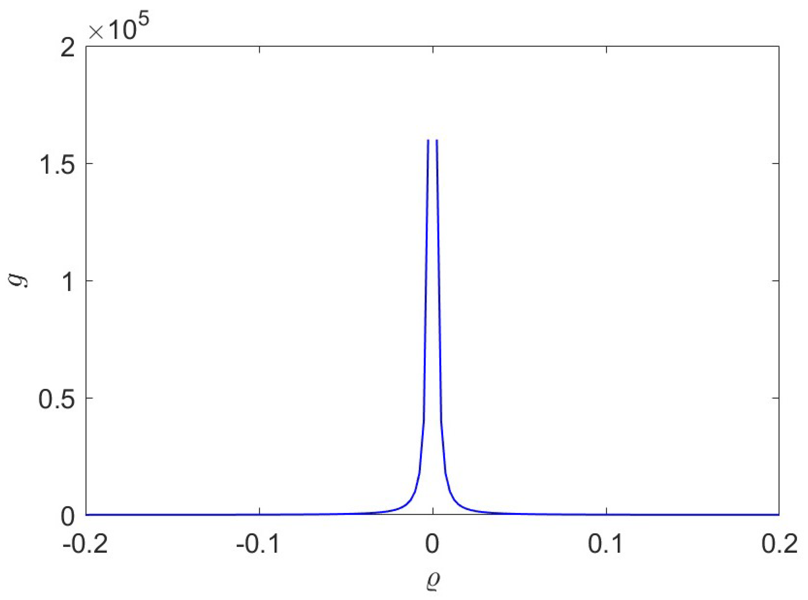
For the Lorentzian manifold ${\mathcal{M}}^4=\{(x,y,z,\varrho ):(x,y,z,\varrho )\in {\mathbb{R}}^4\mathrm{and}\varrho \ne 0\}$ equipped with the metric $g={\displaystyle \frac{1}{{\varrho }^2}}(d{x}^2+d{y}^2+d{z}^2-d{\varrho }^2)$ the graphs in Figure 1 show that the metric components vary inversely with ${\varrho }^2$, indicating a conformally flat behavior of the spacetime geometry.

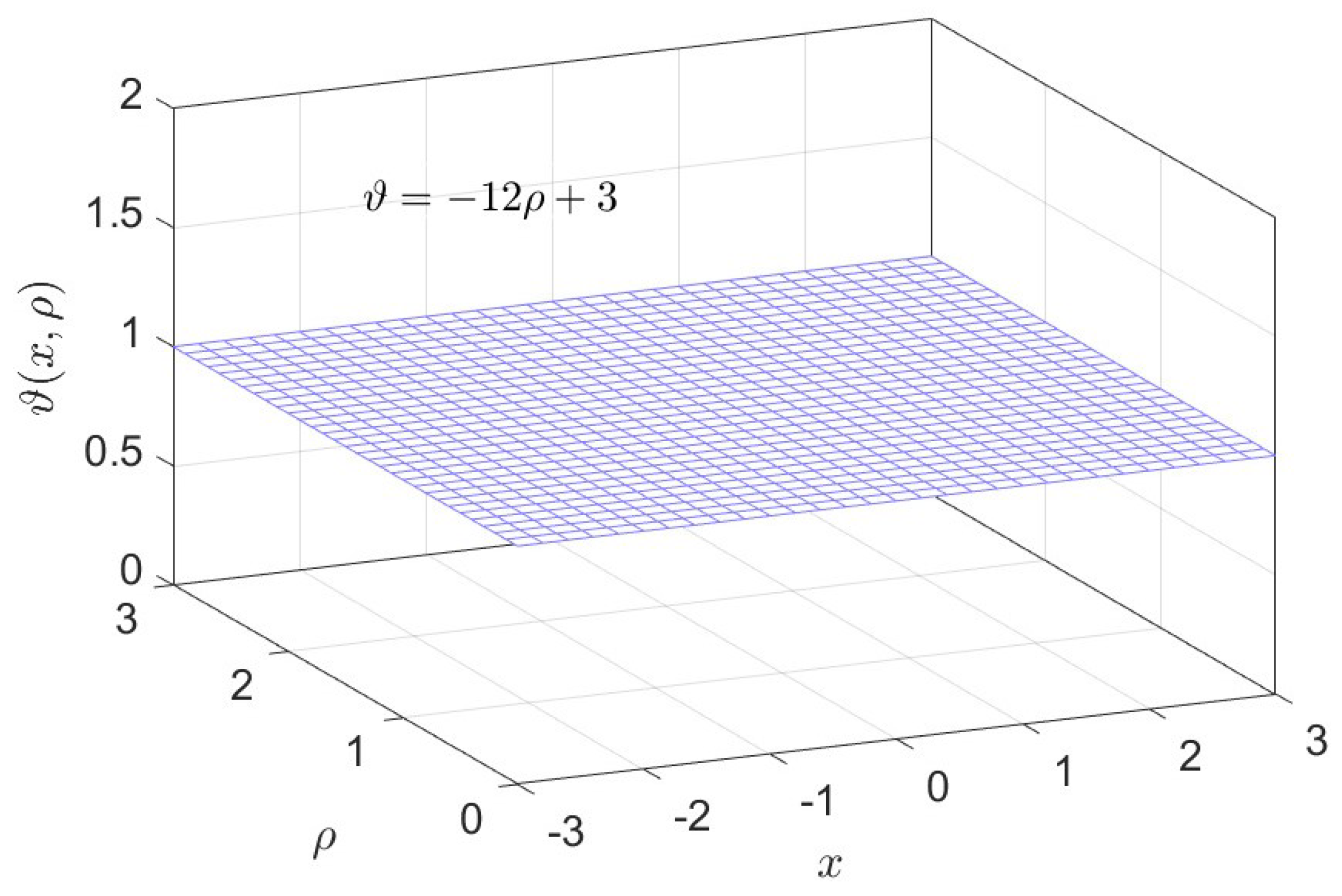
Moreover, the Ricci tensor S satisfies the relation $S=3g$, which confirms that spacetime is Einstein and possesses constant scalar curvature $\tau =12$. In addition, we analyze the equations given in (69) under various choices of parameters. The following Figure 2 illustrates that the solution approaches a stable state when $\vartheta =-12\rho +3$, which is consistent with the theoretical conclusion that $f\in \mathbb{R}$; consequently, the manifold admits a GRBS.

6. Conclusions

The main goal of this manuscript is to investigate general relativistic spacetimes admitting almost Ricci–Bourguignon solitons and gradient almost Ricci–Bourguignon solitons. Several important results have been obtained in the form of theorems, lemmas, and corollaries, which may enrich the existing literature in Lorentzian geometry and mathematical physics. In particular, it is proved that a general relativistic spacetime admitting an ARBS becomes a perfect fluid spacetime. Perfect fluid spacetimes play a fundamental role in general relativity since they provide mathematical models for cosmological matter distributions and relativistic fluid flows. Moreover, the soliton constant is obtained explicitly, which enables us to determine the conditions under which the soliton is expanding, shrinking, or steady. It is also shown that if a perfect fluid spacetime equipped with an ARBS possesses a constant scalar curvature, then the soliton constant satisfies the partial differential equation ${\displaystyle \frac{{\partial }^2\vartheta }{\partial t^2}}-2\vartheta =6(4\rho -1),$ whose solution is given by $\vartheta =A{e}^{\sqrt{2}t}+B{e}^{-\sqrt{2}t}-3(4\rho -1).$ Furthermore, under the same curvature restriction, the ambient spacetime reduces to an Einstein spacetime, and the soliton vector field associated with the ARBS becomes a conformal vector field. Einstein spacetimes are of great importance in differential geometry and general relativity because they represent exact solutions of Einstein’s field equations and describe gravitational models with constant Ricci curvature. In the case of non-constant scalar curvature, it is established that the perfect fluid spacetime admitting an ARBS satisfies the screened Poisson equation. The screened Poisson equation appears naturally in several branches of mathematical physics, including gravitation, diffusion theory, plasma physics, and quantum field theory, where it models screened interactions and potential fields. Conditions characterizing spacetime as subharmonic, superharmonic, and harmonic are also obtained through the associated Laplace equation. The Laplace equation plays a central role in geometry and physics, since harmonic functions describe equilibrium states and potential distributions. A detailed analysis of general relativistic spacetimes admitting gradient almost Ricci–Bourguignon solitons has also been carried out by considering various possible cases. Finally, to support the theoretical findings, a non-trivial example has been constructed which verifies some of the obtained results. The present work also opens several possibilities for future research. Similar investigations may be carried out for other geometric flow structures and generalized Ricci-type solitons on different classes of Lorentzian manifolds such as Sasakian, Kenmotsu, para-contact, and warped product spacetimes. Moreover, the study of ARBS under different curvature conditions, symmetry assumptions, and energy conditions may provide further geometric and physical insights. It would also be interesting to analyze the applications of these structures in cosmological models, gravitational theory, and mathematical physics. Hence, the obtained results may serve as a foundation for further developments in the study of geometric flows and relativistic spacetime geometry.