Hardy Averaging via Distribution Transport: Sharp L^p Bounds, Power Weights, and a Volterra Resolvent

Abstract

Hardy-type averaging operators arise in real analysis, rearrangement theory, weighted inequalities, and Volterra integral equations. This paper develops a distribution-function transport on $(0,\infty )$ equipped with an atomless Borel measure $\mu$, showing that the cumulative map $\Phi \left(x\right)=\mu \left(\right(0,x\left]\right)$ implements a measure isomorphism onto Lebesgue measure under transparent support and continuity hypotheses. Under this transport, the Hardy averaging operator relative to $\mu$ is conjugate to the classical Hardy operator on $(0,\infty )$ with Lebesgue measure. The main contribution is the systematic transport principle: classical constants, extremizing sequences, weighted criteria, endpoint estimates, and resolvent information are transferred exactly to the $\mu$-scale. We establish sharp $L^p\left(\mu \right)$ bounds, sharp power-weight extensions in $L^p\left({\Phi }^{\gamma }d\mu \right)$ for $-1<\gamma <p-1$, a transported one-weight Hardy class beyond powers, endpoint weak and strong estimates, spectral interpretation of the Volterra threshold, and numerical illustrations for the transported constants and a Volterra feedback equation.

1. Introduction

Hardy’s integral inequality begins with the averaging operator

$$\left(Hf\right)\left(y\right)={\displaystyle \frac{1}{y}}{\int }_0^{y}f\left(s\right)ds,y>0,$$

(1)

and the sharp estimate

$${\parallel Hf\parallel }_{L^p(0,\infty )}\le {\displaystyle \frac{p}{p-1}}{\parallel f\parallel }_{L^p(0,\infty )},1<p<\infty .$$

(2)

This operator is one of the basic models for cumulative averaging, weighted embeddings, and one-dimensional reductions of Sobolev and Hardy–Rellich inequalities. Classical sources include the original papers of Hardy and the monograph of Hardy, Littlewood, and Pólya [1,2,3], together with later systematic treatments and extensions [4,5,6,7,8].

The weighted problem asks for conditions on weights $v,w$ such that

$${\left({\int }_0^{\infty }{\left|Hf\left(y\right)\right|}^{q}w\left(y\right)dy\right)}^{1/q}\le C{\left({\int }_0^{\infty }{\left|f\left(y\right)\right|}^{p}v\left(y\right)dy\right)}^{1/p}.$$

(3)

For one-weight and two-weight Hardy inequalities, the sharp qualitative theory is governed by integral testing conditions of Muckenhoupt–Sawyer–Stepanov type [9,10,11]. These criteria sit alongside interpolation and rearrangement principles [12], and they remain a reference point for refined Hardy inequalities with remainder terms and stability mechanisms [13,14,15,16,17].

The present paper studies the following measure-theoretic version. Let $\mu$ be a positive Borel measure on $(0,\infty )$ and set

$$\Phi \left(x\right)=\mu \left(\right(0,x\left]\right).$$

(4)

Whenever $\Phi$ is continuous, strictly increasing, and maps $(0,\infty )$ onto $(0,\infty )$, the change in variables

$$y=\Phi \left(x\right),x=\psi \left(y\right):={\Phi }^{-1}\left(y\right),\left(Uf\right)\left(y\right)=f\left(\psi \left(y\right)\right)$$

(5)

transports $L^p((0,\infty ),\mu )$ isometrically onto $L^p((0,\infty ),dy)$. The Hardy average relative to $\mu$ is

$$\left(H_{\mu }f\right)\left(x\right)={\displaystyle \frac{1}{\Phi \left(x\right)}}{\int }_{(0,x]}f\left(t\right)d\mu \left(t\right),$$

(6)

and the central algebraic identity is the conjugacy

$$U{H}_{\mu }{U}^{-1}=H.$$

(7)

Thus, the paper’s contribution is a transport framework for exact Hardy constants and associated structures on general atomless distribution scales. The classical inequalities supply the constants; the new content is the systematic passage from the Lebesgue scale to the original x-scale, including the precise hypotheses, endpoint forms, weighted interpretations, extremizing sequences, resolvent consequences, and numerical checks in concrete measure models.

This viewpoint is useful in situations where the physical, geometric, or probabilistic variable is x, while cumulative mass $y=\Phi \left(x\right)$ is the natural Hardy scale. Examples include power-growth measures $d{\mu }_{\alpha }\left(x\right)=\alpha x^{\alpha -1}dx$, logarithmic growth $d\mu \left(x\right)=dx/(1+x)$, exponential growth $d{\mu }_{\beta }\left(x\right)=\beta e^{\beta x}dx$, and positive irregular densities. The construction is also connected with the general measure-isomorphism theory of distribution functions and Lebesgue–Stieltjes measures [18]. Recent developments in Hardy theory on variable-exponent spaces, metric-measure spaces, homogeneous groups, and fractional settings provide additional motivation for tracking exactly how constants and weights behave under changes in scale [19,20,21,22,23,24,25,26,27,28,29,30,31,32,33,34,35,36].

The organization is as follows. Section 2 proves the pushforward identity and the operator conjugacy, and it records examples and scope of the standing hypotheses. Section 3 gives the sharp $L^p\left(\mu \right)$ estimate, endpoint statements, power-weight inequalities, and a transported one-weight class beyond powers. Section 4 applies the framework to a Volterra equation and explains the resolvent threshold through the classical Hardy spectrum. Section 5 provides numerical illustrations and a reproducible Python (version 3.14.5) protocol. Section 6 summarizes the transport principle and natural extensions.

2. Preliminaries: Distribution Transport

2.1. Measures and Distribution Functions

Definition 1

(Standing hypothesis). Let μ be a positive Borel measure on $(0,\infty )$ such that $\mu \left(\right(0,x\left]\right)<\infty$ for every $x>0$. Define

$$\Phi \left(x\right)=\mu \left(\right(0,x\left]\right)(x>0).$$

Assume:

$$\begin{array}{cc}\hfill & \left(H1\right)\Phi iscontinuousandstrictlyincreasingon(0,\infty ),\hfill \\ \hfill & \left(H2\right)\underset{x\downarrow 0}{lim}\Phi \left(x\right)=0,\underset{x\uparrow \infty }{lim}\Phi \left(x\right)=\infty .\hfill \end{array}$$

Let $\psi ={\Phi }^{-1}:(0,\infty )\to (0,\infty )$ denote the inverse function.

Remark 1.

(H1) and (H2) imply μ is σ-finite and atomless on $(0,\infty )$. Moreover Φ is a bijection $(0,\infty )\to (0,\infty )$ and ψ is continuous and strictly increasing.

2.2. Pushforward and an $L^p$ Isometry

Lemma 1

(Pushforward of $\mu$ under $\Phi$). Under Definition 1, the pushforward measure ${\Phi }_{\#}\mu$ equals Lebesgue measure $dy$ on $(0,\infty )$. Equivalently, for every Borel set $A\subset (0,\infty )$,

$$\mu \left({\Phi }^{-1}\left(A\right)\right)=\left|A\right|.$$

Proof. 

Let $\nu ={\Phi }_{\#}\mu$ be the pushforward measure on $(0,\infty )$, so $\nu \left(A\right)=\mu \left({\Phi }^{-1}\left(A\right)\right)$ for Borel A. For $y>0$,

$$\nu \left((0,y]\right)=\mu \left({\Phi }^{-1}\left((0,y]\right)\right)=\mu \left((0,\psi (y\left)\right]\right)=\Phi \left(\psi \left(y\right)\right)=y.$$

Thus $\nu \left(\right(0,y\left]\right)=\left|\right(0,y\left]\right|$ for all $y>0$.

Let $\mathcal{D}=\{A\subset (0,\infty )\mathrm{Borel}:\nu (A)=|A\left|\right\}$. Then $\mathcal{D}$ is a Dynkin system: $(0,\infty )\in \mathcal{D}$; if $A\subset B$ with $A,B\in \mathcal{D}$ then $\nu (B\setminus A)=\nu \left(B\right)-\nu \left(A\right)=\left|B\right|-\left|A\right|=|B\setminus A|$; if $\left(A_n\right)$ are disjoint in $\mathcal{D}$ then countable additivity gives $\nu \left({\cup }_n{A}_n\right)={\sum }_n\nu \left(A_n\right)={\sum }_n|A_n|=|{\cup }_n{A}_n|$.

The family $\mathcal{I}=\left\{\right(0,y]:y>0\}$ is a $\pi$-system generating the Borel $\sigma$-algebra of $(0,\infty )$ and satisfies $\mathcal{I}\subset \mathcal{D}$ by the first display. By the $\pi$–$\lambda$ theorem, $\mathcal{D}$ contains all Borel sets. Hence, $\nu \left(A\right)=\left|A\right|$ for all Borel A; that is, ${\Phi }_{\#}\mu =dy$.  □

Lemma 2

(Isometry induced by $\Phi$). Fix $1\le p\le \infty$. Define U by

$$\left(Uf\right)\left(y\right)=f\left(\psi \right(y\left)\right),y>0.$$

Then U is a linear isometry from $L^p((0,\infty ),\mu )$ onto $L^p((0,\infty ),dy)$, with inverse $\left(U^{-1}g\right)\left(x\right)=g(\Phi \left(x\right))$.

Proof. 

Let $1\le p<\infty$. By Lemma 1, for any nonnegative Borel function $\phi$,

$${\int }_0^{\infty }\phi \left(y\right)dy={\int }_{(0,\infty )}\phi (\Phi \left(x\right))d\mu \left(x\right).$$

Apply this with $\phi \left(y\right)={\left|f\left(\psi \left(y\right)\right)\right|}^p$. Since $\psi (\Phi (x\left)\right)=x$, one has $f\left(\psi \right(\Phi \left(x\right)\left)\right)=f\left(x\right)$; hence,

$${\int }_0^{\infty }{\left|Uf\left(y\right)\right|}^{p}dy={\int }_{(0,\infty )}{\left|f\left(\psi (\Phi \left(x\right))\right)\right|}^{p}d\mu \left(x\right)={\int }_{(0,\infty )}{\left|f\left(x\right)\right|}^{p}d\mu \left(x\right).$$

Thus, ${\parallel Uf\parallel }_{L^p\left(dy\right)}={\parallel f\parallel }_{L^p\left(d\mu \right)}$. Surjectivity and the inverse formula follow from the bijectivity of $\Phi$ and $\psi$.

For $p=\infty$, the identity $\left(Uf\right)\circ \Phi =f$ and Lemma 1 imply that sets of $\mu$-measure zero correspond to sets of Lebesgue measure zero under $\Phi$; hence, essential suprema are preserved:

$${\parallel Uf\parallel }_{L^{\infty }\left(dy\right)}={\parallel f\parallel }_{L^{\infty }\left(d\mu \right)}.$$

 □

2.3. Hardy Averaging and Conjugacy

Definition 2

(Hardy averaging relative to $\mu$). Under Definition 1, define $H_{\mu }$ on measurable $f:(0,\infty )\to \mathbb{R}$ by

$$\left(H_{\mu }f\right)\left(x\right)={\displaystyle \frac{1}{\Phi \left(x\right)}}{\int }_{(0,x]}f\left(t\right)d\mu \left(t\right),x>0.$$

Definition 3

(Classical Hardy operator). Define H on measurable $g:(0,\infty )\to \mathbb{R}$ by

$$\left(Hg\right)\left(y\right)={\displaystyle \frac{1}{y}}{\int }_0^{y}g\left(s\right)ds,y>0.$$

Lemma 3

(Conjugacy). For every measurable f and every $y>0$,

$$\left(U{H}_{\mu }f\right)\left(y\right)=H\left(Uf\right)\left(y\right).$$

Equivalently, $U{H}_{\mu }{U}^{-1}=H$ on the natural domains.

Proof. 

Fix $y>0$ and set $x=\psi \left(y\right)$ so that $\Phi \left(x\right)=y$. Define $\tilde{f}\left(t\right)=f\left(t\right){\mathbf{1}}_{(0,x]}\left(t\right)$. Then,

$${\int }_{(0,x]}f\left(t\right)d\mu \left(t\right)={\int }_{(0,\infty )}\tilde{f}\left(t\right)d\mu \left(t\right).$$

Let $g=Uf=f\circ \psi$ and $\tilde{g}=U\tilde{f}=\tilde{f}\circ \psi =g{\mathbf{1}}_{(0,y]}$. By Lemma 2 with $p=1$ applied to $\tilde{f}$,

$${\int }_{(0,\infty )}\tilde{f}\left(t\right)d\mu \left(t\right)={\int }_0^{\infty }\tilde{g}\left(s\right)ds={\int }_0^{y}g\left(s\right)ds.$$

Therefore,

$$\left(U{H}_{\mu }f\right)\left(y\right)=\left(H_{\mu }f\right)\left(\psi \left(y\right)\right)={\displaystyle \frac{1}{\Phi \left(\psi \right(y\left)\right)}}{\int }_{(0,\psi (y\left)\right]}fd\mu ={\displaystyle \frac{1}{y}}{\int }_0^{y}g\left(s\right)ds=H\left(Uf\right)\left(y\right).$$

 □

3. Main Results: Sharp Hardy Bounds on $\mathbf{(}\mathbf{0}\mathbf{,}\mathbf{\infty }\mathbf{,}\mathit{\mu }\mathbf{)}$

3.1. The Classical Sharp Inequality

Lemma 4

(Hardy inequality on Lebesgue measure). Let $1<p<\infty$ and $g\in L^p((0,\infty ),dy)$. Then,

$${\parallel Hg\parallel }_{L^p\left((0,\infty )\right)}\le {\displaystyle \frac{p}{p-1}}{\parallel g\parallel }_{L^p\left((0,\infty )\right)}.$$

The constant ${\displaystyle \frac{p}{p-1}}$ is optimal.

Proof. 

Since $\left|Hg\right|\le H\left|g\right|$ pointwise by linearity and positivity of the averaging kernel, it suffices to treat $g\ge 0$. Define

$$G\left(y\right)={\int }_0^{y}g\left(s\right)ds,y>0,$$

so G is absolutely continuous on compact intervals and $G^{\prime }\left(y\right)=g\left(y\right)$ for almost every y.

Fix $R>0$ and set

$$I_R={\int }_0^R{\left({\displaystyle \frac{G\left(y\right)}{y}}\right)}^{p}dy={\int }_0^{R}G{\left(y\right)}^p{y}^{-p}dy.$$

The boundary term at $y=0$ vanishes: by Hölder on $(0,y)$,

$$G\left(y\right)={\int }_0^{y}g\left(s\right)ds\le {\left({\int }_0^{y}g{\left(s\right)}^{p}ds\right)}^{1/p}{y}^{1-1/p};$$

hence,

$$0\le G{\left(y\right)}^p{y}^{1-p}\le {\int }_0^{y}g{\left(s\right)}^{p}ds⟶0\mathrm{as}y\downarrow 0.$$

Integrating by parts with $u\left(y\right)=G{\left(y\right)}^p$ and $dv=y^{-p}dy$ (so $du=pG{\left(y\right)}^{p-1}g\left(y\right)dy$ and $v\left(y\right)={\displaystyle \frac{y^{1-p}}{1-p}}$) yields

$$\begin{array}{cc}\hfill I_R& ={\left[{\displaystyle \frac{G{\left(y\right)}^p{y}^{1-p}}{1-p}}\right]}_{y=0}^{y=R}-{\int }_0^R{\displaystyle \frac{y^{1-p}}{1-p}}pG{\left(y\right)}^{p-1}g\left(y\right)dy\hfill \\ \hfill & ={\displaystyle \frac{G{\left(R\right)}^p{R}^{1-p}}{1-p}}+{\displaystyle \frac{p}{p-1}}{\int }_0^R{\left({\displaystyle \frac{G\left(y\right)}{y}}\right)}^{p-1}g\left(y\right)dy.\hfill \end{array}$$

Because $1-p<0$ and $G{\left(R\right)}^p{R}^{1-p}\ge 0$, the term ${\displaystyle \frac{G{\left(R\right)}^p{R}^{1-p}}{1-p}}\le 0$; hence,

$$I_R\le {\displaystyle \frac{p}{p-1}}{\int }_0^R{\left({\displaystyle \frac{G\left(y\right)}{y}}\right)}^{p-1}g\left(y\right)dy.$$

Apply Hölder’s inequality on $(0,R)$ with exponents ${\displaystyle \frac{p}{p-1}}$ and p:

$${\int }_0^R{\left({\displaystyle \frac{G\left(y\right)}{y}}\right)}^{p-1}g\left(y\right)dy\le {\left({\int }_0^R{\left({\displaystyle \frac{G\left(y\right)}{y}}\right)}^{p}dy\right)}^{{\displaystyle \frac{p-1}{p}}}{\left({\int }_0^{R}g{\left(y\right)}^{p}dy\right)}^{{\displaystyle \frac{1}{p}}}=I_R^{{\displaystyle \frac{p-1}{p}}}{\parallel g\parallel }_{L^p(0,R)}.$$

Combining gives

$$I_R\le {\displaystyle \frac{p}{p-1}}{I}_R^{{\displaystyle \frac{p-1}{p}}}{\parallel g\parallel }_{L^p(0,R)},$$

and since $I_R\ge 0$, this yields

$$I_R^{1/p}\le {\displaystyle \frac{p}{p-1}}{\parallel g\parallel }_{L^p(0,R)}.$$

Letting $R\uparrow \infty$ and using monotone convergence yields

$${\parallel Hg\parallel }_{L^p\left((0,\infty )\right)}\le {\displaystyle \frac{p}{p-1}}{\parallel g\parallel }_{L^p\left((0,\infty )\right)}.$$

To prove optimality, define for $\epsilon >0$

$$g_{\epsilon }\left(y\right)=y^{-1/p}{\left(log(e/y)\right)}^{-1/p-\epsilon }{\mathbf{1}}_{(0,1)}\left(y\right).$$

A change in variables $t=log(e/y)$ gives

$${\parallel g_{\epsilon }\parallel }_{L^p}^p={\int }_0^1{y}^{-1}{\left(log(e/y)\right)}^{-1-p\epsilon }dy={\int }_1^{\infty }{t}^{-1-p\epsilon }dt={\displaystyle \frac{1}{p\epsilon }}.$$

For $y\in (0,1)$,

$$\begin{array}{cc}\hfill \left(H{g}_{\epsilon }\right)\left(y\right)& ={\displaystyle \frac{1}{y}}{\int }_0^y{s}^{-1/p}{\left(log(e/s)\right)}^{-1/p-\epsilon }ds\hfill \\ \hfill & =y^{-1/p}{\int }_0^1{r}^{-1/p}{\left(log(e/y)+log(1/r)\right)}^{-1/p-\epsilon }dr,\hfill \end{array}$$

using $s=yr$. For each fixed $r\in (0,1)$, the ratio

$${\left(1+{\displaystyle \frac{log(1/r)}{log(e/y)}}\right)}^{-1/p-\epsilon }⟶1\mathrm{as}y\downarrow 0.$$

Moreover, for $y\in (0,1)$ and $r\in (0,1)$,

$$0\le r^{-1/p}{\left(log(e/y)+log(1/r)\right)}^{-1/p-\epsilon }\le r^{-1/p}{\left(log(e/y)\right)}^{-1/p-\epsilon },$$

and ${\int }_0^1{r}^{-1/p}dr={\displaystyle \frac{p}{p-1}}<\infty$. Dominated convergence therefore yields

$$\underset{y\downarrow 0}{lim}{\displaystyle \frac{\left(H{g}_{\epsilon }\right)\left(y\right)}{g_{\epsilon }\left(y\right)}}={\displaystyle \frac{p}{p-1}}=:C_p.$$

Fix $\eta \in (0,1)$ and choose $\delta \in (0,1)$ such that

$$\left(H{g}_{\epsilon }\right)\left(y\right)\ge (C_p-\eta )g_{\epsilon }\left(y\right)\mathrm{for}\mathrm{all}y\in (0,\delta ).$$

Then,

$${\parallel H{g}_{\epsilon }\parallel }_{L^p}^p\ge {\int }_0^{\delta }|H{g}_{\epsilon }{\left(y\right)|}^{p}dy\ge {(C_p-\eta )}^p{\int }_0^{\delta }{\left|g_{\epsilon }\left(y\right)\right|}^{p}dy.$$

Since ${\int }_0^1{\left|g_{\epsilon }\right|}^p={\displaystyle \frac{1}{p\epsilon }}$ and ${\int }_{\delta }^1{\left|g_{\epsilon }\right|}^{p}dy$ stays bounded as $\epsilon \downarrow 0$ (it converges to ${\int }_{\delta }^1{y}^{-1}{(log(e/y))}^{-1}dy<\infty$),

$${\displaystyle \frac{{\int }_0^{\delta }{\left|g_{\epsilon }\right|}^p}{{\int }_0^1{\left|g_{\epsilon }\right|}^p}}⟶1\mathrm{as}\epsilon \downarrow 0.$$

Consequently,

$$\underset{\epsilon \downarrow 0}{lim\; inf}{\displaystyle \frac{\parallel H{g}_{\epsilon }{\parallel }_{L^p}}{\parallel g_{\epsilon }{\parallel }_{L^p}}}\ge C_p-\eta .$$

Since $\eta$ is arbitrary and the proved inequality gives the matching upper bound ${\parallel H{g}_{\epsilon }\parallel }_{L^p}/{\parallel g_{\epsilon }\parallel }_{L^p}\le C_p$, one gets

$$\underset{\epsilon \downarrow 0}{lim}{\displaystyle \frac{\parallel H{g}_{\epsilon }{\parallel }_{L^p}}{\parallel g_{\epsilon }{\parallel }_{L^p}}}=C_p,$$

which forces optimality of $C_p={\displaystyle \frac{p}{p-1}}$.  □

3.2. Sharp $L^p\left(\mu \right)$ Bound via Conjugacy

Theorem 1

(Sharp $L^p\left(\mu \right)$ Hardy bound). Assume Definition 1 and let $1<p<\infty$. Then, for every $f\in L^p((0,\infty ),\mu )$,

$$\parallel H_{\mu }{f\parallel }_{L^p((0,\infty ),\mu )}\le {\displaystyle \frac{p}{p-1}}{\parallel f\parallel }_{L^p((0,\infty ),\mu )}.$$

The constant ${\displaystyle \frac{p}{p-1}}$ is optimal. An extremizing family is

$$f_{\epsilon }\left(x\right)=\Phi {\left(x\right)}^{-1/p}{\left(log(e/\Phi (x\left)\right)\right)}^{-1/p-\epsilon }{\mathbf{1}}_{\{\Phi (x)<1\}}\left(x\right),\epsilon >0.$$

Proof. 

Let $f\in L^p\left(\mu \right)$ and set $g=Uf=f\circ \psi$. By Lemma 2,

$${\parallel f\parallel }_{L^p\left(\mu \right)}={\parallel g\parallel }_{L^p\left(dy\right)}.$$

By Lemma 3, $U{H}_{\mu }f=Hg$, hence again by Lemma 2,

$$\parallel H_{\mu }{f\parallel }_{L^p\left(\mu \right)}=\parallel U{H}_{\mu }{f\parallel }_{L^p\left(dy\right)}={\parallel Hg\parallel }_{L^p\left(dy\right)}.$$

Apply Lemma 4 to obtain

$$\parallel H_{\mu }{f\parallel }_{L^p\left(\mu \right)}\le {\displaystyle \frac{p}{p-1}}{\parallel g\parallel }_{L^p\left(dy\right)}={\displaystyle \frac{p}{p-1}}{\parallel f\parallel }_{L^p\left(\mu \right)}.$$

For sharpness, let $g_{\epsilon }$ be the extremizing family from Lemma 4 and define $f_{\epsilon }=U^{-1}{g}_{\epsilon }=g_{\epsilon }\circ \Phi$. Then, $U{f}_{\epsilon }=g_{\epsilon }$ and $U{H}_{\mu }{f}_{\epsilon }=H{g}_{\epsilon }$, so

$${\displaystyle \frac{\parallel H_{\mu }{f}_{\epsilon }{\parallel }_{L^p\left(\mu \right)}}{\parallel f_{\epsilon }{\parallel }_{L^p\left(\mu \right)}}}={\displaystyle \frac{\parallel H{g}_{\epsilon }{\parallel }_{L^p\left(dy\right)}}{\parallel g_{\epsilon }{\parallel }_{L^p\left(dy\right)}}}⟶{\displaystyle \frac{p}{p-1}}\mathrm{as}\epsilon \downarrow 0,$$

which forces optimality of the constant on $(0,\infty ,\mu )$.  □

3.3. Endpoint Forms

Proposition 1

(Endpoint estimates). Assume Definition 1.

1. 

For $f\in L^{\infty }((0,\infty ),\mu )$,

$$\parallel H_{\mu }{f\parallel }_{L^{\infty }\left(\mu \right)}\le {\parallel f\parallel }_{L^{\infty }\left(\mu \right)},$$

(8)

with sharp constant 1.

2. 

For $f\in L^1((0,\infty ),\mu )$ and $a>0$,

$$\mu \left(\{x>0:|H_{\mu }f\left(x\right)|>a\}\right)\le {\displaystyle \frac{1}{a}}{\parallel f\parallel }_{L^1\left(\mu \right)}.$$

(9)

The strong $L^1\left(\mu \right)$ inequality has no finite global constant on $(0,\infty )$.

Proof. 

Let $g=Uf$. For $p=\infty$, Lemma 3 and the elementary estimate $\left|Hg\left(y\right)\right|\le {\parallel g\parallel }_{\infty }$ give

$$\parallel H_{\mu }{f\parallel }_{\infty }={\parallel Hg\parallel }_{\infty }\le {\parallel g\parallel }_{\infty }={\parallel f\parallel }_{\infty }.$$

Taking constant functions on finite $\mu$-measure intervals and passing to larger intervals gives the sharpness of constant 1.

For the weak $L^1$ estimate, the classical weak-type bound for H gives

$$\left|\right\{y>0:\left|Hg\left(y\right)\right|>a\left\}\right|\le a^{-1}{\parallel g\parallel }_1.$$

The pushforward identity converts this directly into (9). Finally, choose $g={\mathbf{1}}_{(0,1)}$. Then $Hg\left(y\right)=1$ for $0<y<1$ and $Hg\left(y\right)=1/y$ for $y\ge 1$; hence, $Hg\notin L^1(0,\infty )$ while $g\in L^1(0,\infty )$. Pulling back g by $U^{-1}$ proves the corresponding assertion on $(0,\infty ,\mu )$.  □

3.4. Sharp Power-Weight Extensions

Lemma 5

(Weighted Hardy inequality on Lebesgue measure). Let $1<p<\infty$ and let γ satisfy $-1<\gamma <p-1$. Define the weight $w_{\gamma }\left(y\right)=y^{\gamma }$. Then, for every $g\in L^p((0,\infty ),w_{\gamma }dy)$,

$${\parallel Hg\parallel }_{L^p((0,\infty ),w_{\gamma }dy)}\le {\displaystyle \frac{p}{p-1-\gamma }}{\parallel g\parallel }_{L^p((0,\infty ),w_{\gamma }dy)}.$$

The constant ${\displaystyle \frac{p}{p-1-\gamma }}$ is optimal.

Proof. 

As before, it suffices to treat $g\ge 0$ since $\left|Hg\right|\le H\left|g\right|$. Let $G\left(y\right)={\int }_0^{y}g\left(s\right)ds$ and fix $R>0$. Set

$$I_R={\int }_0^R{\left({\displaystyle \frac{G\left(y\right)}{y}}\right)}^p{y}^{\gamma }dy={\int }_0^{R}G{\left(y\right)}^p{y}^{\gamma -p}dy.$$

The boundary term at $y=0$ vanishes. By Hölder on $(0,y)$ with weights $s^{\gamma /p}$ and $s^{-\gamma /p}$,

$$G\left(y\right)={\int }_0^{y}g\left(s\right)ds={\int }_0^y\left(g\left(s\right)s^{\gamma /p}\right)s^{-\gamma /p}ds\le {\left({\int }_0^{y}g{\left(s\right)}^p{s}^{\gamma }ds\right)}^{1/p}{\left({\int }_0^y{s}^{-\gamma /(p-1)}ds\right)}^{(p-1)/p}.$$

Since $-1<\gamma <p-1$, the exponent $-\gamma /(p-1)>-1$ and

$${\int }_0^y{s}^{-\gamma /(p-1)}ds={\displaystyle \frac{y^{1-\gamma /(p-1)}}{1-\gamma /(p-1)}}.$$

Therefore, there exists a constant $C_{p,\gamma }>0$ such that

$$G{\left(y\right)}^p\le C_{p,\gamma }{y}^{p-1-\gamma }{\int }_0^{y}g{\left(s\right)}^p{s}^{\gamma }ds.$$

Multiplying by $y^{\gamma +1-p}$ yields

$$0\le G{\left(y\right)}^p{y}^{\gamma +1-p}\le C_{p,\gamma }{\int }_0^{y}g{\left(s\right)}^p{s}^{\gamma }ds⟶0\mathrm{as}y\downarrow 0.$$

Integrate by parts with $u\left(y\right)=G{\left(y\right)}^p$ and $dv=y^{\gamma -p}dy$. Since $\gamma +1-p=-(p-1-\gamma )$,

$$v\left(y\right)={\displaystyle \frac{y^{\gamma +1-p}}{\gamma +1-p}},du=pG{\left(y\right)}^{p-1}g\left(y\right)dy,$$

so

$$\begin{array}{cc}\hfill I_R& ={\left[{\displaystyle \frac{G{\left(y\right)}^p{y}^{\gamma +1-p}}{\gamma +1-p}}\right]}_{y=0}^{y=R}-{\int }_0^R{\displaystyle \frac{y^{\gamma +1-p}}{\gamma +1-p}}pG{\left(y\right)}^{p-1}g\left(y\right)dy\hfill \\ \hfill & ={\displaystyle \frac{G{\left(R\right)}^p{R}^{\gamma +1-p}}{\gamma +1-p}}+{\displaystyle \frac{p}{p-1-\gamma }}{\int }_0^R{\left({\displaystyle \frac{G\left(y\right)}{y}}\right)}^{p-1}g\left(y\right)y^{\gamma }dy.\hfill \end{array}$$

Because $\gamma +1-p<0$ and $G{\left(R\right)}^p{R}^{\gamma +1-p}\ge 0$, the first term is $\le 0$; hence,

$$I_R\le {\displaystyle \frac{p}{p-1-\gamma }}{\int }_0^R{\left({\displaystyle \frac{G\left(y\right)}{y}}\right)}^{p-1}g\left(y\right)y^{\gamma }dy.$$

Apply Hölder on $(0,R)$ with measure $y^{\gamma }dy$:

$${\int }_0^R{\left({\displaystyle \frac{G\left(y\right)}{y}}\right)}^{p-1}g\left(y\right)y^{\gamma }dy\le I_R^{{\displaystyle \frac{p-1}{p}}}{\parallel g\parallel }_{L^p((0,R),y^{\gamma }dy)}.$$

Thus,

$$I_R^{1/p}\le {\displaystyle \frac{p}{p-1-\gamma }}{\parallel g\parallel }_{L^p((0,R),y^{\gamma }dy)}.$$

Let $R\uparrow \infty$ to obtain the inequality.

For optimality, define for $\epsilon >0$

$$g_{\epsilon ,\gamma }\left(y\right)=y^{-(\gamma +1)/p}{\left(log(e/y)\right)}^{-1/p-\epsilon }{\mathbf{1}}_{(0,1)}\left(y\right).$$

Then,

$${\parallel g_{\epsilon ,\gamma }\parallel }_{L^p\left(y^{\gamma }dy\right)}^p={\int }_0^1{y}^{-(\gamma +1)}{(log(e/y))}^{-1-p\epsilon }{y}^{\gamma }dy={\int }_0^1{y}^{-1}{(log(e/y))}^{-1-p\epsilon }dy={\displaystyle \frac{1}{p\epsilon }}.$$

An argument identical in structure to the sharpness proof in Lemma 4 (with $r^{-1/p}$ replaced by $r^{-(\gamma +1)/p}$, which is integrable on $(0,1)$ exactly when $\gamma <p-1$) yields

$$\underset{\epsilon \downarrow 0}{lim}{\displaystyle \frac{\parallel H{g}_{\epsilon ,\gamma }{\parallel }_{L^p\left(y^{\gamma }dy\right)}}{\parallel g_{\epsilon ,\gamma }{\parallel }_{L^p\left(y^{\gamma }dy\right)}}}={\displaystyle \frac{p}{p-1-\gamma }},$$

forcing optimality of the constant.  □

Theorem 2

(Sharp power-weight inequality on $(0,\infty ,\mu )$). Assume Definition 1. Let $1<p<\infty$ and $-1<\gamma <p-1$. Then for every $f\in L^p((0,\infty ),{\Phi }^{\gamma }d\mu )$,

$$\parallel H_{\mu }{f\parallel }_{L^p((0,\infty ),{\Phi }^{\gamma }d\mu )}\le {\displaystyle \frac{p}{p-1-\gamma }}{\parallel f\parallel }_{L^p((0,\infty ),{\Phi }^{\gamma }d\mu )}.$$

The constant ${\displaystyle \frac{p}{p-1-\gamma }}$ is optimal. A sharpness family is

$$f_{\epsilon ,\gamma }\left(x\right)=\Phi {\left(x\right)}^{-(\gamma +1)/p}{\left(log(e/\Phi (x\left)\right)\right)}^{-1/p-\epsilon }{\mathbf{1}}_{\{\Phi (x)<1\}}\left(x\right),\epsilon >0.$$

Proof. 

Let $f\in L^p\left({\Phi }^{\gamma }d\mu \right)$ and set $g=Uf=f\circ \psi$. Using Lemma 1,

$${\int }_{(0,\infty )}{\left|f\left(x\right)\right|}^p\Phi {\left(x\right)}^{\gamma }d\mu \left(x\right)={\int }_0^{\infty }{\left|f\left(\psi \left(y\right)\right)\right|}^p{y}^{\gamma }dy={\int }_0^{\infty }{\left|g\left(y\right)\right|}^p{y}^{\gamma }dy,$$

hence ${\parallel f\parallel }_{L^p\left({\Phi }^{\gamma }d\mu \right)}={\parallel g\parallel }_{L^p\left(y^{\gamma }dy\right)}$. By Lemma 3, $U{H}_{\mu }f=Hg$, so similarly

$$\parallel H_{\mu }{f\parallel }_{L^p\left({\Phi }^{\gamma }d\mu \right)}={\parallel Hg\parallel }_{L^p\left(y^{\gamma }dy\right)}.$$

Apply Lemma 5 to obtain the desired bound.

For sharpness, take $g_{\epsilon ,\gamma }$ from Lemma 5 and set $f_{\epsilon ,\gamma }=U^{-1}{g}_{\epsilon ,\gamma }=g_{\epsilon ,\gamma }\circ \Phi$. Then, the norm ratio on $(0,\infty ,\mu )$ equals the norm ratio on $(0,\infty ,dy)$, which tends to ${\displaystyle \frac{p}{p-1-\gamma }}$ as $\epsilon \downarrow 0$.  □

4. Application: A Volterra Equation Driven by Hardy Averaging

Theorem 3

(Resolvent estimate for $u=g+\lambda H_{\mu }u$). Assume Definition 1 and fix $1<p<\infty$. Let $g\in L^p((0,\infty ),\mu )$ and $\lambda \in \mathbb{R}$ satisfy

$$\left|\lambda \right|<{\displaystyle \frac{p-1}{p}}.$$

Then, the equation

$$u=g+\lambda H_{\mu }u$$

has a unique solution $u\in L^p((0,\infty ),\mu )$ given by the convergent Neumann series

$$u={\displaystyle \sum _{n=0}^{\infty }}{\lambda }^n{H}_{\mu }^{n}g,$$

and the solution satisfies the bound

$${\parallel u\parallel }_{L^p\left(\mu \right)}\le {\displaystyle \frac{1}{1-\left|\lambda \right|\frac{p}{p-1}}}{\parallel g\parallel }_{L^p\left(\mu \right)}.$$

Proof. 

Theorem 1 yields ${\parallel H_{\mu }\parallel }_{L^p\left(\mu \right)\to L^p\left(\mu \right)}\le {\displaystyle \frac{p}{p-1}}$; hence, for each $n\ge 1$,

$$\parallel H_{\mu }^n{g\parallel }_{L^p\left(\mu \right)}\le {\left({\displaystyle \frac{p}{p-1}}\right)}^n{\parallel g\parallel }_{L^p\left(\mu \right)}.$$

Therefore, the series ${\sum }_{n\ge 0}{\lambda }^n{H}_{\mu }^{n}g$ converges absolutely in $L^p\left(\mu \right)$ whenever $\left|\lambda \right|{\displaystyle \frac{p}{p-1}}<1$, which is the hypothesis. Let

$$u={\displaystyle \sum _{n=0}^{\infty }}{\lambda }^n{H}_{\mu }^{n}g\mathrm{in}{L}^p\left(\mu \right).$$

Because $H_{\mu }$ is bounded on $L^p\left(\mu \right)$, one may apply $H_{\mu }$ termwise to obtain convergence of

$$H_{\mu }u={\displaystyle \sum _{n=0}^{\infty }}{\lambda }^n{H}_{\mu }^{n+1}g\mathrm{in}{L}^p\left(\mu \right).$$

Then,

$$g+\lambda H_{\mu }u=g+{\displaystyle \sum _{n=0}^{\infty }}{\lambda }^{n+1}{H}_{\mu }^{n+1}g={\displaystyle \sum _{n=0}^{\infty }}{\lambda }^n{H}_{\mu }^{n}g=u,$$

so u solves the equation.

For uniqueness, if $u_1,u_2\in L^p\left(\mu \right)$ satisfy $u_i=g+\lambda H_{\mu }{u}_i$, then $v=u_1-u_2$ satisfies $v=\lambda H_{\mu }v$; hence,

$${\parallel v\parallel }_{L^p\left(\mu \right)}\le \left|\lambda \right|\parallel H_{\mu }{v\parallel }_{L^p\left(\mu \right)}\le \left|\lambda \right|{\displaystyle \frac{p}{p-1}}{\parallel v\parallel }_{L^p\left(\mu \right)}.$$

Since $\left|\lambda \right|{\displaystyle \frac{p}{p-1}}<1$, this forces ${\parallel v\parallel }_{L^p\left(\mu \right)}=0$.

Finally, the norm estimate follows from the geometric series bound:

$$\begin{array}{cc}\hfill {\parallel u\parallel }_{L^p\left(\mu \right)}& \le {\displaystyle \sum _{n=0}^{\infty }}{\left|\lambda \right|}^n\parallel H_{\mu }^n{g\parallel }_{L^p\left(\mu \right)}\le {\displaystyle \sum _{n=0}^{\infty }}{\left|\lambda \right|}^n{\left({\displaystyle \frac{p}{p-1}}\right)}^n{\parallel g\parallel }_{L^p\left(\mu \right)}\hfill \\ \hfill & ={\displaystyle \frac{1}{1-\left|\lambda \right|\frac{p}{p-1}}}{\parallel g\parallel }_{L^p\left(\mu \right)}.\hfill \end{array}$$

 □

Remark 2

(Explicit transported form). Let $v=Ug$ and $z=Uu$. The Volterra equation becomes

$$z\left(y\right)=v\left(y\right)+{\displaystyle \frac{\lambda }{y}}{\int }_0^{y}z\left(s\right)ds.$$

(10)

Writing $F\left(y\right)={\int }_0^{y}z\left(s\right)ds$ gives the first-order equation

$$F^{\prime }\left(y\right)-{\displaystyle \frac{\lambda }{y}}F\left(y\right)=v\left(y\right),F\left(0\right)=0.$$

(11)

For inputs for which the integral is finite, this gives

$$F\left(y\right)=y^{\lambda }{\int }_0^y{s}^{-\lambda }v\left(s\right)ds,z\left(y\right)=v\left(y\right)+\lambda y^{\lambda -1}{\int }_0^y{s}^{-\lambda }v\left(s\right)ds.$$

(12)

The solution in the original variable is $u\left(x\right)=z(\Phi (x\left)\right)$.

Remark 3

(Resolvent threshold and spectrum). The operator identity $U{H}_{\mu }{U}^{-1}=H$ implies

$$U{(I-\lambda H_{\mu })}^{-1}{U}^{-1}={(I-\lambda H)}^{-1}$$

(13)

whenever either side exists. Hence the Volterra threshold is governed by the classical Cesàro–Hardy spectrum. On $L^p(0,\infty )$, $1<p<\infty$, the spectrum of H is the closed disk

$$\sigma \left(H\right)=\left\{z\in \mathbb{C}:\left|z-{\displaystyle \frac{p^{\prime }}{2}}\right|\le {\displaystyle \frac{p^{\prime }}{2}}\right\},p^{\prime }={\displaystyle \frac{p}{p-1}},$$

(14)

as in the classical theory of Cesàro operators [33]. The Neumann condition $\left|\lambda \right|<1/p^{\prime }=(p-1)/p$ is therefore the open disk guaranteed by the norm estimate. Along the positive real axis, $\lambda \uparrow 1/p^{\prime }$ approaches a spectral boundary point and the resolvent norm diverges. The compactness intuition belongs to the unnormalised finite-interval Volterra map $Vf\left(x\right)={\int }_0^{x}f\left(t\right)dt$; the normalized Hardy map $H_{\mu }$ retains dilation invariance after transport and compactness fails on the infinite scale.

5. Numerical Illustrations and Volterra Experiment

This section records reproducible numerical checks of the transported constants and of the Volterra resolvent. The computations use no external data. The examples are designed to verify the mechanism of the proofs on finite quadrature windows and to illustrate the behavior near the critical Hardy threshold.

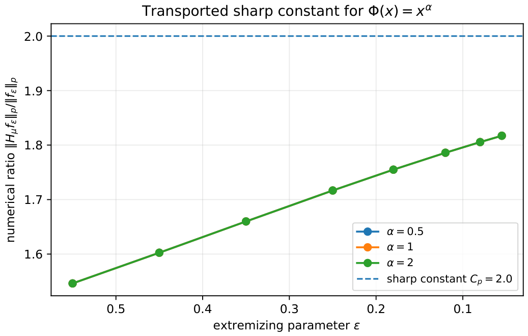
For the first experiment, take

$$\Phi \left(x\right)=x^{\alpha },d{\mu }_{\alpha }\left(x\right)=\alpha x^{\alpha -1}dx,\alpha >0.$$

(15)

For $p=2$, the transported extremizing family is

$$f_{\epsilon }\left(x\right)=\Phi {\left(x\right)}^{-1/2}{\left(log(e/\Phi (x\left)\right)\right)}^{-1/2-\epsilon }{\mathbf{1}}_{\{\Phi (x)<1\}}.$$

(16)

Figure 1 shows the numerical ratio ${\parallel H_{\mu }{f}_{\epsilon }{\parallel }_2/\parallel f_{\epsilon }\parallel }_2$ for several values of $\alpha$. The curves coincide up to quadrature error, as predicted by the isometry, and move toward the sharp constant $C_2=2$ as $\epsilon$ decreases.

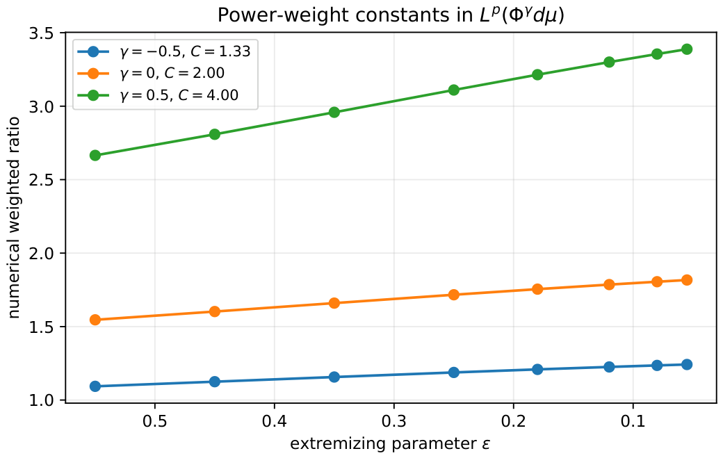
The second experiment tests the power-weight theorem. For $p=2$ and $\gamma \in \{-1/2,0,1/2\}$, the theoretical constants are $2/(1-\gamma )$, namely $4/3$, 2, and 4. Figure 2 shows the corresponding finite-window norm ratios for weighted extremizing sequences.

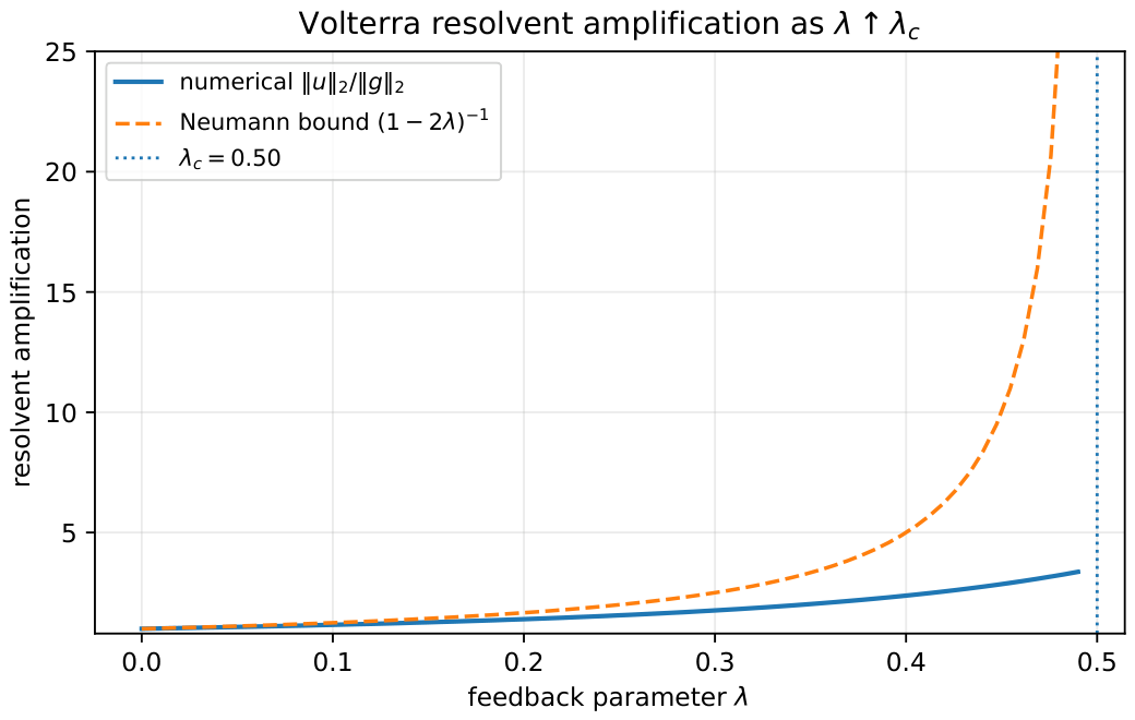
For the Volterra experiment, the transported Equation (10) is solved for

$$v\left(y\right)=e^{-y}\left(1+0.15cos\left(2y\right)\right),p=2,$$

(17)

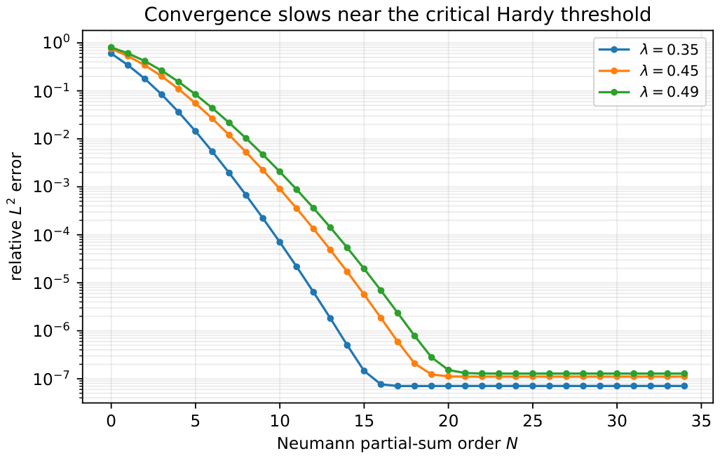
using the explicit Formula (12). Figure 3 compares the observed amplification ${\parallel u\parallel }_2/{\parallel g\parallel }_2$ with the Neumann bound ${(1-2\lambda )}^{-1}$ as $\lambda$ approaches the critical value ${\lambda }_c=1/2$. Figure 4 shows that the Neumann partial sums converge more slowly near the same threshold.

Next, we present representative numerical values obtained from the transport and Volterra experiments in

Table 1. Representative numerical values from the transport and Volterra experiments are given below. In the first two blocks, the last column is the sharp theoretical constant; in the Volterra block, it is the Neumann resolvent bound.

Test	Parameters	Numerical Value	Reference Value
unweighted	$p=2,\alpha =2,\epsilon =0.250$	1.716709	2.000000
unweighted	$p=2,\alpha =2,\epsilon =0.120$	1.785958	2.000000
unweighted	$p=2,\alpha =2,\epsilon =0.055$	1.817166	2.000000
weighted	$p=2,\gamma =-0.5,\epsilon =0.055$	1.242115	1.333333
weighted	$p=2,\gamma =0,\epsilon =0.055$	1.817166	2.000000
weighted	$p=2,\gamma =0.5,\epsilon =0.055$	3.387999	4.000000
Volterra	$p=2,\lambda =0.45$	2.827636	9.504132
Volterra	$p=2,\lambda =0.49$	3.367764	50.000000

.

The numerical study is illustrative. The proof of the constants is analytic and independent of the quadrature. The finite computational window truncates both the singular region near $y=0$ and the tail $y=\infty$, so the extremizing ratios approach the theoretical constants from below. Refining the logarithmic mesh and expanding the integration window improves agreement, while the qualitative transport invariance and the Volterra threshold behavior are already visible at the resolutions used here.

6. Conclusions and Future Directions

This paper establishes a distribution-function transport that converts Hardy averaging on $(0,\infty )$ with respect to an atomless Borel measure $\mu$ into the classical Hardy operator on Lebesgue measure. The principal contribution is the exact transfer method: once $y=\Phi \left(x\right)$ is used as the cumulative variable, sharp constants, endpoint estimates, extremizing sequences, weighted criteria, and Volterra resolvent bounds are inherited from the classical Hardy theory with no loss in the optimal operator norm.

The sharp unweighted estimate gives ${\parallel H_{\mu }\parallel }_{p\to p}=p/(p-1)$ for $1<p<\infty$, the endpoint theory gives a sharp $L^{\infty }$ contraction and a weak $L^1$ estimate, and the weighted result gives the sharp power constant $p/(p-1-\gamma )$ in $L^p\left({\Phi }^{\gamma }d\mu \right)$. The transported class $B_{p,\Phi }$ extends the theory beyond powers and gives a direct route to Muckenhoupt–Hardy-type weights on the original measure scale. For the Volterra equation, the condition $\left|\lambda \right|<(p-1)/p$ is the Neumann resolvent regime dictated by the transported Hardy norm, while the classical Cesàro spectrum explains the critical behavior along the positive real axis.

Natural extensions include two-weight inequalities in the transported class, fractional Hardy averages in the $\Phi$ variable, rearrangement-invariant refinements, and quotient/generalized-inverse formulations for atomless measures with zero-mass gaps. Measures with atoms lead to Lebesgue–Stieltjes target measures and require a separate discrete–continuous Hardy theory.

References

- Hardy, G.H. Note on a theorem of Hilbert. Math. Z. 1920, 6, 314–317. [Google Scholar] [CrossRef]
- Hardy, G.H. Notes on some points in the integral calculus, LX. An inequality between integrals. Messenger Math. 1925, 54, 150–156. [Google Scholar]
- Hardy, G.H.; Littlewood, J.E.; Pólya, G. Inequalities; Cambridge University Press: Cambridge, UK, 1934. [Google Scholar]
- Beesack, P.R. Hardy’s inequality and its extensions. Pac. J. Math. 1961, 11, 39–61. [Google Scholar] [CrossRef]
- Opic, B.; Kufner, A. Hardy-Type Inequalities; Longman Scientific & Technical: Harlow, UK, 1990. [Google Scholar]
- Kufner, A.; Persson, L.-E. Weighted Inequalities of Hardy Type; World Scientific: Singapore, 2003. [Google Scholar]
- Kufner, A.; Maligranda, L.; Persson, L.-E. The prehistory of the Hardy inequality. Am. Math. Mon. 2006, 113, 715–732. [Google Scholar] [CrossRef]
- Kufner, A.; Maligranda, L.; Persson, L.-E. The Hardy Inequality: About Its History and Some Related Results; Vydavatelský Servis: Pilsen, Czech Republic, 2007. [Google Scholar]
- Muckenhoupt, B. Hardy’s inequality with weights. Stud. Math. 1972, 44, 31–38. [Google Scholar] [CrossRef]
- Sawyer, E.T. Weighted Lebesgue and Lorentz norm inequalities for the Hardy operator. Trans. Am. Math. Soc. 1984, 281, 329–337. [Google Scholar] [CrossRef]
- Sinnamon, G.; Stepanov, V.D. The weighted Hardy inequality: New proofs and the case p = 1. J. Lond. Math. Soc. 1996, 54, 89–101. [Google Scholar] [CrossRef]
- Bennett, C.; Sharpley, R. Interpolation of Operators; Academic Press: Boston, MA, USA, 1988. [Google Scholar]
- Davies, E.B. The Hardy constant. Q. J. Math. 1995, 46, 417–431. [Google Scholar] [CrossRef]
- Brezis, H.; Marcus, M. Hardy’s inequalities revisited. Ann. Sc. Norm. Super. Pisa Cl. Sci. 1997, 25, 217–237. [Google Scholar]
- Barbatis, G.; Filippas, S.; Tertikas, A. A unified approach to improved Lp Hardy inequalities with best constants. Trans. Am. Math. Soc. 2004, 356, 2169–2196. [Google Scholar] [CrossRef]
- Cianchi, A.; Ferone, A. Hardy inequalities with nonstandard remainder terms. Ann. L’Institut Henri Poincaré Anal. Non Linéaire 2008, 25, 889–906. [Google Scholar] [CrossRef]
- Frank, R.L.; Seiringer, R. Non-linear ground state representations and sharp Hardy inequalities. J. Funct. Anal. 2008, 255, 3407–3430. [Google Scholar] [CrossRef]
- Bogachev, V.I. Measure Theory; Springer: Berlin/Heidelberg, Germany, 2007; Volumes I–II. [Google Scholar]
- Frank, R.L.; Merz, K. On Sobolev norms involving Hardy operators in a half-space. J. Funct. Anal. 2023, 285, 110104. [Google Scholar] [CrossRef]
- Wani, S.A.; Riyasat, M.; Khan, S.; Ramírez, W. Certain advancements in multidimensional q-Hermite polynomials. Rep. Math. Phys. 2024, 94, 117–141. [Google Scholar] [CrossRef]
- Cruz-Uribe, D.; Suragan, D. Hardy–Leray inequalities in variable Lebesgue spaces. J. Math. Anal. Appl. 2024, 530, 127747. [Google Scholar] [CrossRef]
- Kassymov, A.; Ruzhansky, M.; Suragan, D. Reverse integral Hardy inequality on metric measure spaces. Ann. Fenn. Math. 2022, 47, 39–55. [Google Scholar] [CrossRef]
- Ruzhansky, M.; Shriwastawa, A.; Tiwari, B. A note on best constants for weighted integral Hardy inequalities on homogeneous groups. Results Math. 2024, 79, 29. [Google Scholar] [CrossRef]
- Sultan, A.; Sultan, S. Boundedness of higher order commutators of Hardy operators on grand Herz–Morrey spaces. Bull. Sci. Math. 2024, 190, 103373. [Google Scholar] [CrossRef]
- Wani, S.A.; Abuasbeh, K.; Oros, G.I.; Trabelsi, S. Degenerate 2D bivariate Appell polynomials: Properties and applications. Appl. Math. Sci. Eng. 2023, 31, 2194645. [Google Scholar] [CrossRef]
- Cinti, E.; Prinari, F. On fractional Hardy-type inequalities in general open sets. ESAIM Control Optim. Calc. Var. 2024, 30, 77. [Google Scholar] [CrossRef]
- Ihnatsyeva, L.; Mohanta, K.; Vähäkangas, A.V. Fractional Hardy inequalities and capacity density. arXiv 2024, arXiv:2404.05222. [Google Scholar] [CrossRef]
- Zayed, M.; Wani, S.A.; Quintana, Y. Properties of multivariate Hermite polynomials in correlation with Frobenius–Euler polynomials. Mathematics 2023, 11, 3439. [Google Scholar] [CrossRef]
- Kassymov, A.; Ruzhansky, M.; Zaur, G. On fractional inequalities on metric measure spaces with polar decomposition. arXiv 2024, arXiv:2407.15197. [Google Scholar] [CrossRef]
- Bandaliyev, R.A.; Aliyev, M.G.; Agarzayev, B.K. On reverse Hardy inequality in variable Lebesgue spaces. J. Math. Inequal. 2025, 19, 821–837. [Google Scholar] [CrossRef]
- Asim, M.; Suwais, K.; Mlaiki, N. Some new weighted results for the Hardy operator on variable-exponent λ-central Morrey space. Eur. J. Pure Appl. Math. 2025, 18, 6667. [Google Scholar] [CrossRef]
- Gogatishvili, A.; Ünver, A. Weighted inequalities involving two Hardy operators. Anal. Math. Phys. 2025, 15, 99. [Google Scholar] [CrossRef]
- Brown, A.; Halmos, P.R.; Shields, A.L. Cesaro operators. Acta Sci. Math. 1965, 26, 125–137. [Google Scholar]
- Maz’ya, V.G. Sobolev Spaces: With Applications to Elliptic Partial Differential Equations, 2nd ed.; Springer: Berlin/Heidelberg, Germany, 2011. [Google Scholar]
- Wani, S.A.; Khan, S.; Naikoo, S.A. Differential and integral equations for the Laguerre–Gould–Hopper-based Appell and related polynomials. Bol. Soc. Mat. Mex. 2020, 26, 617–646. [Google Scholar] [CrossRef]
- Gripenberg, G.; Londen, S.-O.; Staffans, O. Volterra Integral and Functional Equations; Cambridge University Press: Cambridge, UK, 1990. [Google Scholar]