Article

A Chaos-Based Image Encryption Algorithm via Integrated Cellular Automata and Tent Map Systems

1
School of Computer Science and Technology, Changsha University of Science and Technology, Changsha 410076, China
2
School of Physics and Electronic Science, Changsha University of Science and Technology, Changsha 410114, China
3
School of Information and Electrical Engineering, Hunan University of Science and Technology, Xiangtan 411201, China
*
Author to whom correspondence should be addressed.
Axioms 2026, 15(5), 304; https://doi.org/10.3390/axioms15050304
Submission received: 3 February 2026 / Revised: 14 April 2026 / Accepted: 15 April 2026 / Published: 23 April 2026
(This article belongs to the Special Issue Nonlinear Dynamical System and Its Applications)

Abstract

This study proposes a novel image encryption algorithm based on a two-dimensional discrete chaotic system that integrates cellular automata (CA) with a tent map. The algorithm addresses security vulnerabilities in digital image transmission and storage across open networks or cloud environments. It employs a three-phase encryption process: coordinate permutation, spatial permutation, and diffusion. Sequential application of Arnold’s coordinate scrambling, maze traversal-based spatial rearrangement, and a CA-driven diffusion mechanism enhances robustness against noise, differential attacks, and partial cropping. A Dynamic CA–Tent Map (DCA–TM) hybrid chaotic system is designed to overcome periodicity and limited key space issues inherent in conventional chaotic encryption. The permutation stage is refined into coordinate and spatial phases to achieve comprehensive pixel randomization. During diffusion, CA rules are selected dynamically based on the iteration counts of the initial parameters, yielding an adaptive encryption system with a variable key space. Performance evaluations—including Lyapunov exponent tests, bifurcation analysis, information entropy measurement, and pixel correlation assessment—confirm the strong chaotic behavior and high security of the proposed scheme.
MSC:
34C28; 65P20; 94A08; 65D18

1. Introduction

The rapid advancement and widespread deployment of next-generation information technologies—such as big data [1,2,3], neural computing [4,5,6], artificial intelligence [7,8,9], and data networks [10,11,12]—have introduced increasingly complex security challenges. Among various forms of digital content, image data serves as a critical information carrier, and its secure transmission has become a prominent research focus in network communication. Compared with structured textual data, digital images exhibit strong spatial correlation among adjacent pixels and high information redundancy [13,14,15,16]. As a result, conventional text-oriented encryption standards such as AES and DES are inefficient when directly applied to images, often causing substantial ciphertext expansion and residual visual patterns [17,18,19]. Consequently, specialized image encryption techniques have emerged, with chaotic systems being a favored solution due to their unique dynamical properties [20,21,22,23].
Chaotic systems fall into two broad categories: continuous and discrete. Continuous chaotic systems, described by differential equations, are suitable for high-precision simulations [24,25]. Notable examples include the atmospheric convection model proposed by Lorenz [26] and its subsequent Matlab2021b/FPGA implementations [27,28,29,30]. Hyperchaotic systems, a subclass of continuous chaos characterized by multiple positive Lyapunov exponents, can generate highly complex pseudo-random sequences [31,32,33,34].
Discrete chaotic systems, implemented via iterative maps, exhibit comparatively simpler dynamics yet offer high computational efficiency and ease of hardware realization [35,36,37,38,39]. The universality of the logistic map, established by May and Feigenbaum in the 1970s, laid the theoretical groundwork, while its application to real-time image encryption was later demonstrated by Alvarez et al. [40]. The use of chaotic maps for image encryption originated with Matthews’ seminal work in 1989 [41], which proved that the ergodicity of the tent map satisfies Kerckhoffs’s principle. Subsequent research has progressed along two primary directions. The first involves dimension expansion, exemplified by Huang et al.’s composite chaotic system that elevates a 1D logistic map to higher dimensions, increasing the Lyapunov exponent by a factor of 3.2 through phase-space folding [42]. The second direction focuses on hybrid architectures, including Tutueva et al.’s adaptive symmetric chaotic framework [43] (which expands the parameter space by 2 32 times compared to traditional methods) and Zarebnia et al.’s parallel encryption scheme based on Arnold’s cat map [44]. Notably, Fridrich’s investigation of the 2D Baker map revealed that scrambling efficiency improves by over 40% when the chaotic system’s dimension matches that of the image [45]. This body of work underscores a key characteristic of chaotic cryptography: discrete chaotic systems are well-suited for practical image encryption due to their simplicity and low computational overhead [46,47,48].
Cellular automata (CA) have also been validated for cryptographic use since Wolfram demonstrated the pseudo-randomness of Rule 30 in 1986 [49]. Recent advances center on three aspects. First, rule optimization: Nandi et al. showed that alternating Rule 90 and Rule 150 produces sequences that pass all NIST tests [50]. Second, architectural innovation: Chen et al. developed a reversible hybrid CA achieving encryption speeds of 1.2 μs per pixel [51]. Third, system integration: a notable example is the three-stage encryption scheme by Wang et al., which combines DNA encoding, CA, and chaotic mapping and exhibits key sensitivity down to 10 28  [52]. Moreover, the partitioned cellular automata method proposed by Wang et al. markedly improved encryption efficiency [53], and Niyat et al.’s integration of hyperchaotic systems with CA offers a promising approach for color image encryption [54]. Despite these advancements, two limitations persist. First, the use of static CA rules confines the rule-space entropy to at most log 2 ( 256 ) = 8 bits [55,56,57], which is a negligible contribution to the overall key space. Second, the coupling between chaotic systems and CA in existing schemes is predominantly a simple cascade: the CA acts as a post-processor on the output of a chaotic map, without any feedback or dynamic interaction between the two subsystems [58,59,60]. In essence, the chaotic trajectory and the CA evolution remain largely independent, thereby under-utilizing the potential synergistic complexity that could arise from their mutual influence. The present work departs fundamentally from this cascade paradigm. Rather than treating CA as a static downstream component, we embed the CA rule-selection mechanism directly into the iterative dynamics of the tent map. Specifically, the frequency and pattern of CA rule switching are governed in real time by the chaotic state variables themselves. This deep coupling ensures that the system’s trajectory is not merely the output of a chaotic map followed by a deterministic cellular automaton, but a co-evolving hybrid state in which the continuous chaotic phase space and the discrete CA rule space continuously reshape one another.
Regarding security analysis, various attacks on chaotic image encryption algorithms have been reported. Bokhari et al. identified vulnerabilities in hybrid systems through cryptanalysis of quantum chaotic maps and DNA encoding [61], and Feng et al. performed systematic cryptanalysis of schemes relying on pixel-level filtering and DNA diffusion [62]. These studies underscore the necessity of designing more robust hybrid encryption methods.
To address the aforementioned challenges, this work introduces a Dynamic CA–Tent Map (DCA-TM) hybrid system. Its key innovations include: (1) linking the frequency of CA rule switching to the dynamics of the tent map, thereby expanding the key space from 2 8 to 2 135 ; (2) designing a maze traversal spatial scrambling algorithm that reformulates image permutation as a graph traversal problem; and (3) constructing a dynamic-rule CA diffusion mechanism that enables linear scalability of both key space and security strength.
The remainder of this paper is organized as follows. Section 2 presents the DCA–TM hybrid chaotic system, detailing its dynamical characteristics—including Lyapunov exponents, bifurcation behavior, and NIST randomness tests—and compares it with classical chaotic systems. Section 3 introduces a breadth-first search (BFS)-based pixel scrambling method that globally randomizes pixel positions through simulated maze traversal, along with an analysis of its resistance to statistical attacks. Section 4 describes the three-stage encryption process (coordinate scrambling, spatial scrambling, and diffusion), covering the Arnold transform, maze traversal scrambling, dynamic CA diffusion, and reversible decryption. Section 5 validates the algorithm’s security and robustness through key space evaluation, correlation analysis, information entropy tests, and assessments of resilience to noise and cropping attacks, with comparisons to existing schemes.

2. A Novel Chaotic System Based on Cellular Automata and Tent Map

Chaos refers to a class of deterministic yet seemingly random dynamical behaviors observed in many natural systems. In this work, chaotic mappings are defined as nonlinear dynamical systems exhibiting extreme sensitivity to initial conditions. Prior research demonstrates that efficient encryption systems can be constructed from canonical chaotic maps, notably the tent map and elementary cellular automata (ECA). This section first analyzes the dynamical properties of the tent map and ECA, then it proposes a new chaotic system built through nonlinear coupling. The chaotic nature of the proposed system is rigorously validated via numerical experiments.

2.1. Tent Map

The tent map was first proposed by Soviet mathematician A.N. Sharkovsky in the 1960s during his research on dynamical systems, and it was later extensively analyzed and popularized in chaos theory by American mathematician Robert L. Devaney and others. Its name derives from the tent-like shape of its function graph. When the parameter is equal to 2, the map exhibits fully developed chaos, making it a classic model for studying sensitivity to initial conditions and ergodicity. Its simple piecewise linear form has been widely applied in pseudo-random number generation and encryption algorithms, serving as a quintessential example of “simple systems producing chaotic behavior.”
The standard form of the tent map is:
T μ ( x ) = μ x , 0 x 1 2 , μ ( 1 x ) , 1 2 < x 1 .

2.2. Cellular Automata

Cellular Automata (CA), originally proposed by John von Neumann and Stanislaw Ulam in the 1940s, were initially conceived to model biological self-replication. This computational framework consists of four fundamental components: a discrete lattice of cells, a finite set of states, a neighborhood definition, and a transition rule. John Conway’s Game of Life (1970) later demonstrated how simple local rules could generate complex emergent behaviors. Stephen Wolfram [63] systematically classified CA dynamics into four categories and established the Turing completeness of certain CA variants. As discrete dynamical systems defined in space, time, and state, CA exhibit rich global behaviors through localized interactions, making them widely applicable in physics (e.g., fluid dynamics), biology (e.g., morphogenesis), and social systems (e.g., traffic flow modeling). In cryptography, CA’s parallel computability and sensitivity to initial conditions enable efficient encryption schemes. Within complexity science, CA serve as essential tools for studying self-organization, edge-of-chaos phenomena, and other nonlinear dynamics. Over decades of development, CA theory has profoundly influenced interdisciplinary research, bridging mathematics, computer science, and complex systems studies.
In elementary cellular automata, the state update of each cell is determined by its own state and the states of its neighbors at the previous time step, and the local transition function can be expressed in the following mathematical form:
S i ( t + 1 ) = f S i 1 t , S i t , S i + 1 t
Here, S i t denotes the state of the cell at position i at time step t, and f represents the local rule of the cellular automaton. For an elementary cellular automaton, the neighborhood consists of three cells, each with only two possible states. Thus, there are 2 3 = 8 possible input state combinations. Since each input can produce one of two possible output states, there are a total of 2 8 = 256 possible rules. The rule number is determined by the decimal equivalent of the binary sequence representing the output states. Table 1 shows the state transition table corresponding to Rule 75.

2.3. Dynamic CA–Tent Map

This work proposes a novel chaotic system (DCA–TM) based on the integration of cellular automata and tent mapping. The system significantly enhances the performance of conventional tent mapping through three key innovations. Firstly, it introduces CA’s local evolution rules and modified Logistic transformation to achieve dual nonlinear processing of state variables. Secondly, it replaces the fixed parameter μ with a dynamic parameter p and directly incorporates it into the piecewise conditions of the mapping. Finally, through designed coupling coefficients and cross-feedback mechanisms, it constructs a two-dimensional phase space with excellent ergodicity. The core formula of the DCA–TM system is presented as follows:
x n + 1 = p 6 · L M C A ( x n , i ) + y n , if x n < p p 4 · L M C A ( y n , i ) + x n , if x n p y n + 1 = p 4 · L M C A ( x n , i ) + y n , if x n < p p 6 · L M C A ( y n , i ) + x n , if x n p
The system state variables x n and y n represent the two-dimensional state values at the n-th iteration of the chaotic system, with their values constrained to the interval [ 0 , 1 ] , forming the basis of the two-dimensional phase space. The parameter p serves as the key control parameter, which not only replaces the fixed parameter μ in Equation (4) but is also directly embedded in the piecewise conditions ( x n < p or x n p ) to achieve dynamic regulation. CA denotes the evolution rules of cellular automata, whose output depends on both the current state value ( x n or y n ) and the iteration count i of the elementary cellular automaton. The operator L M represents a fractal-enhanced Logistic mapping, defined as:
L M fractal ( x ) = μ fractal ( x ) · ( 3 x + 1 ) · x · ( 1 x ) ,
where the modulation parameter μ fractal ( x ) is given by
μ fractal ( x ) = 1.85 × 1 + sin 2 π · Ψ ( x ) 4 ,
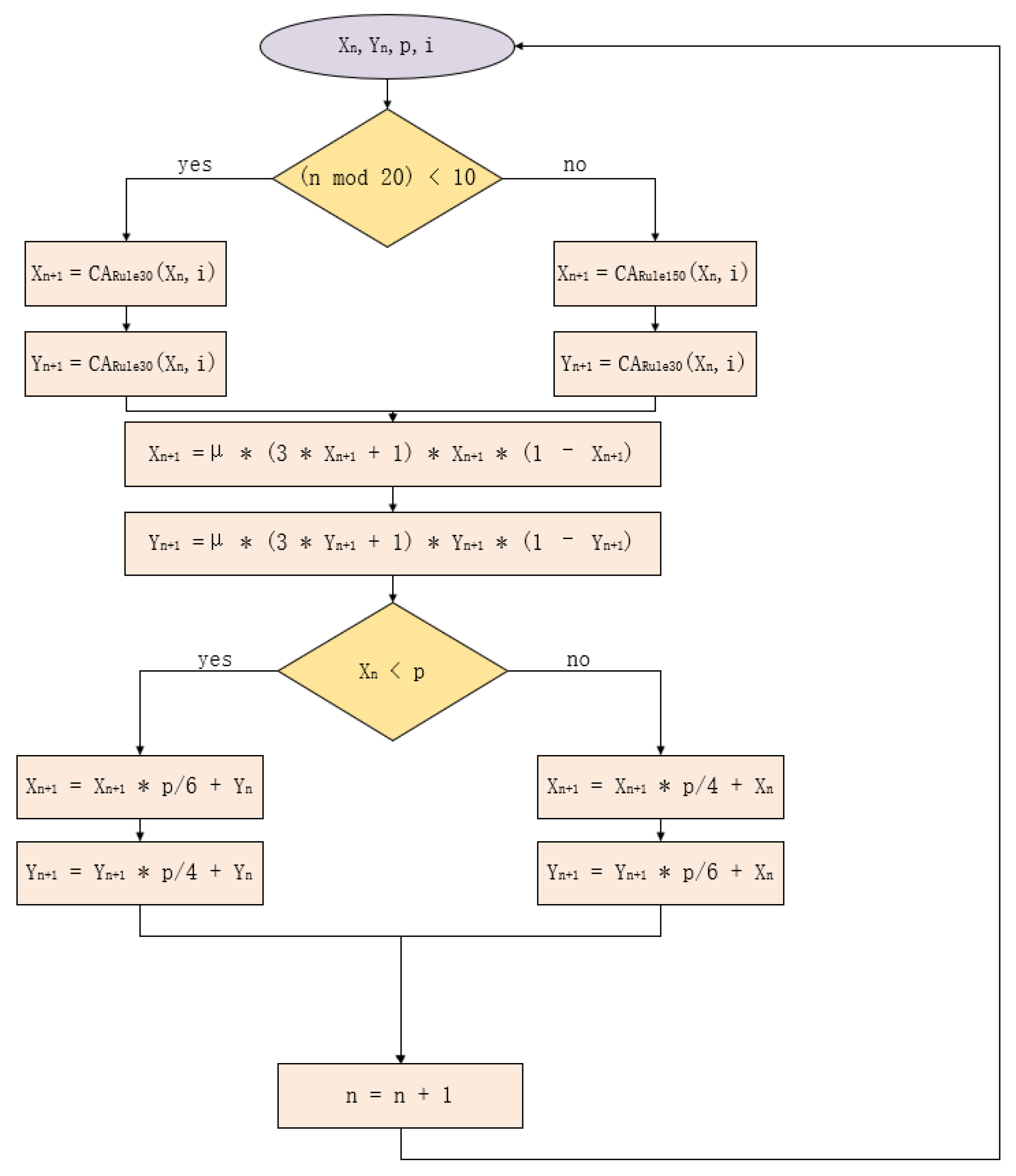
and Ψ ( x ) : [ 0 , 1 ] [ 0 , 1 ] is a fractal localization function defined by the pseudo-code in Algorithm 1. This fractal structure ensures that even tiny differences in the input x lead to significantly different outputs, effectively eliminating sparse orbital regions that may appear when the control parameter p is small, while preserving the original system architecture. The fractal approach follows the methodology introduced in earlier works on right-hand side fractal functions in chaotic systems [64]. The CA alternates between two rules: Rule 30 and Rule 150, with the rule switching every ten iterations of the chaotic system. The generation process of the output sequence for the DCA–TM chaotic system is shown in Figure 1.
Algorithm 1 Fractal localization function Ψ ( x )
Input:  x [ 0 , 1 ] , depth d (e.g., d = 10 )
Output:  Ψ ( x ) [ 0 , 1 ]
 1: s t e p 2 d
 2: k x / s t e p  {Index of subinterval}
 3: Ψ ( x ) k × s t e p   Ψ ( x )

2.3.1. Bifurcation Analysis

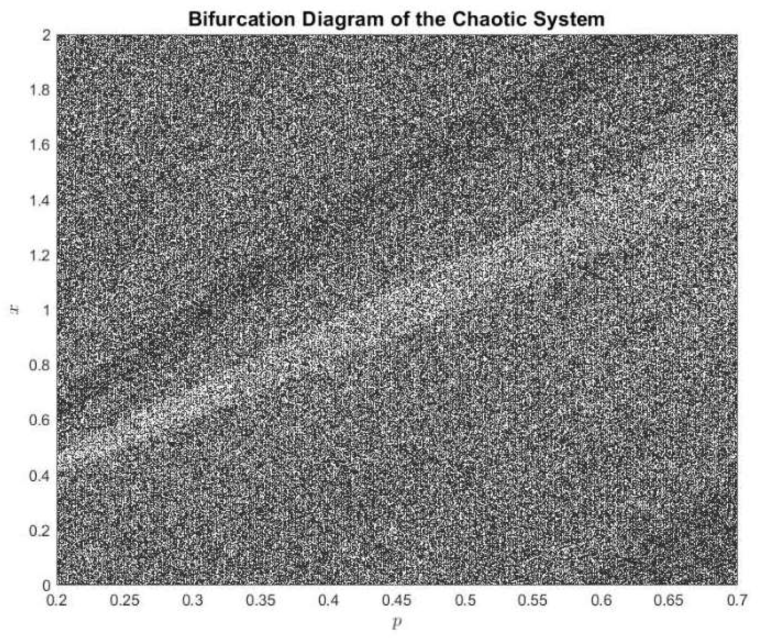
The bifurcation diagram constitutes an essential analytical tool in nonlinear dynamics, enabling systematic examination of chaotic system properties. As shown in Figure 2, it provides visual representation of parameter-dependent system behaviors while distinctly illustrating both stability conditions and chaotic regime distributions. Our analysis of the Dynamic CA–Tent Map (DCA–TM) system reveals that the high density of chaotic trajectories and their uniform phase-space distribution (see Figure 2) collectively demonstrate the robust chaotic characteristics and dynamical stability inherent to this proposed system.

2.3.2. Lyapunov Exponent Comparison

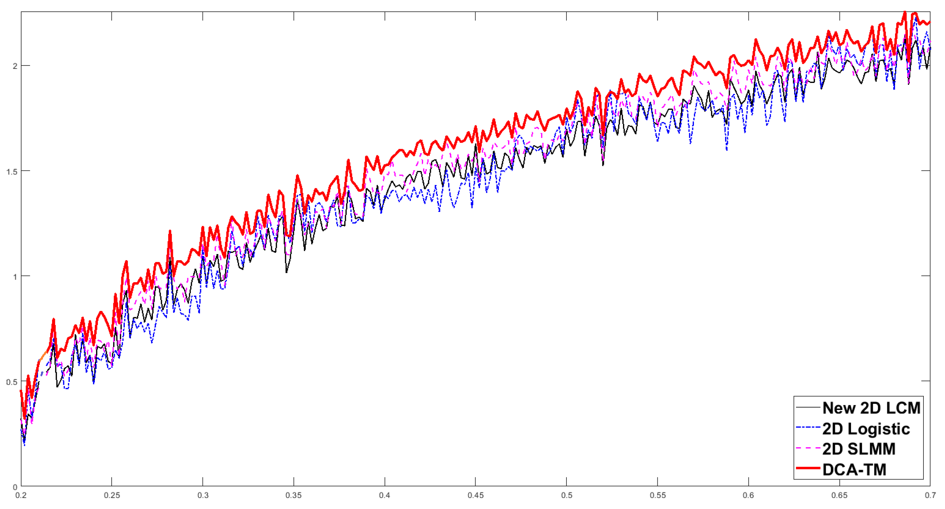
Figure 3 presents a comparative analysis of Lyapunov exponent (LE) metrics between DCA–TM and several conventional chaotic systems. The results demonstrate that DCA–TM achieves significantly higher LE values, indicating superior chaotic sensitivity and enhanced dynamic complexity compared to benchmark systems. This quantitative evidence confirms the improved chaotic characteristics of our proposed system.

2.3.3. NIST Test

The NIST test suite comprises 15 comprehensive tests, requiring all test results to be greater than or equal to 0.01. It is designed to evaluate the randomness quality of binary sequences generated by hardware or software, regardless of their length. Within the context of chaotic systems, these tests play a critical role in assessing the performance of random number generators, particularly in fields such as cryptography and information security. By passing these tests, the system effectively demonstrates that the generated data exhibits high randomness and unpredictability.
As illustrated in Table 2, the system successfully passed all 15 tests, confirming that its chaotic mechanism is capable of producing data with strong randomness.

2.3.4. 0–1 Test

The 0–1 test for chaos is a binary test that distinguishes between regular and chaotic dynamics in deterministic systems. Given a scalar time series { ϕ ( j ) } j = 1 N , the test computes a value K close to 0 for regular dynamics and close to 1 for chaotic dynamics. For a random constant c ( 0 , π ) , we define translation components:
D c ( n ) = 1 N j = 1 N n p c ( j + n ) p c ( j ) 2 + q c ( j + n ) q c ( j ) 2 1 N j = 1 N ϕ ( j ) 2 1 cos ( n c ) 1 cos ( c ) ,
and its growth rate with respect to n yields the correlation coefficient K c . The final test outcome K is the median of K c over many randomly chosen c (typically c ( π / 5 , 4 π / 5 ) ).
We applied the 0–1 test to the pseudo-random sequences generated by the DCA–TM system. Specifically, we used the x-component of the chaotic output (after discarding a sufficient number of initial transients) as the input series ϕ ( j ) with length N = 10 5 . The median value of K c over 100 randomly chosen c was found to be K = 0.996 , which is extremely close to 1. This result confirms the strongly chaotic nature of the DCA–TM system and is consistent with the high Lyapunov exponents and the successful NIST tests reported in previous subsections, further validating the excellent randomness of the generated sequences.

3. Maze Traversal-Based Spatial Scrambling Algorithm

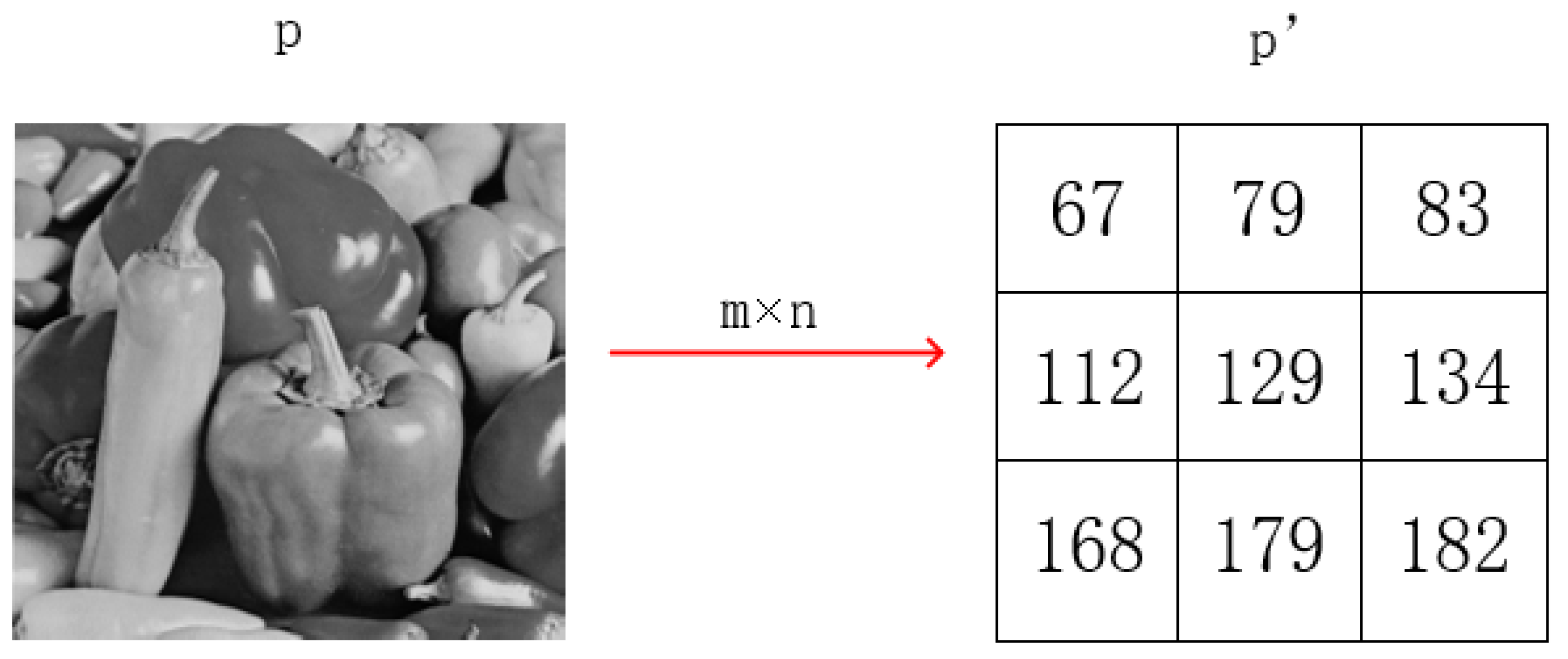
The second stage of the encryption process employs a spatial scrambling algorithm based on maze traversal. This algorithm rearranges the pixel matrix by simulating navigation through a maze, thereby achieving spatial scrambling of the image. Consider an m × n image matrix P derived from the original image P, as shown in Figure 4.
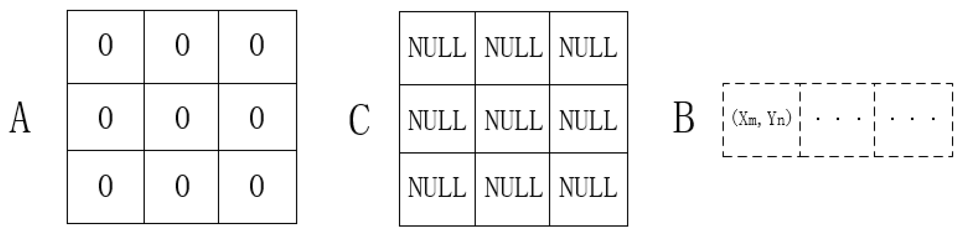
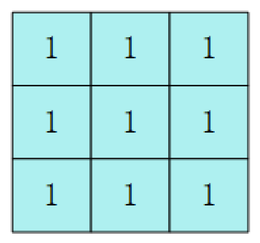
Step 1: Create a Boolean access marker matrix A of the same dimensions as the original image, initialized to 0, to track whether each coordinate has been visited.(see Figure 5).
Create coordinate sequence matrix B ( N × 2 , N: total pixels) where ( X m , Y n ) are coordinates to be added, storing traversed coordinate pairs in order; initialized as empty. Create an encrypted image matrix C, with the same dimensions and data type as the original image, initialized as a zero matrix, used to store the encryption results.
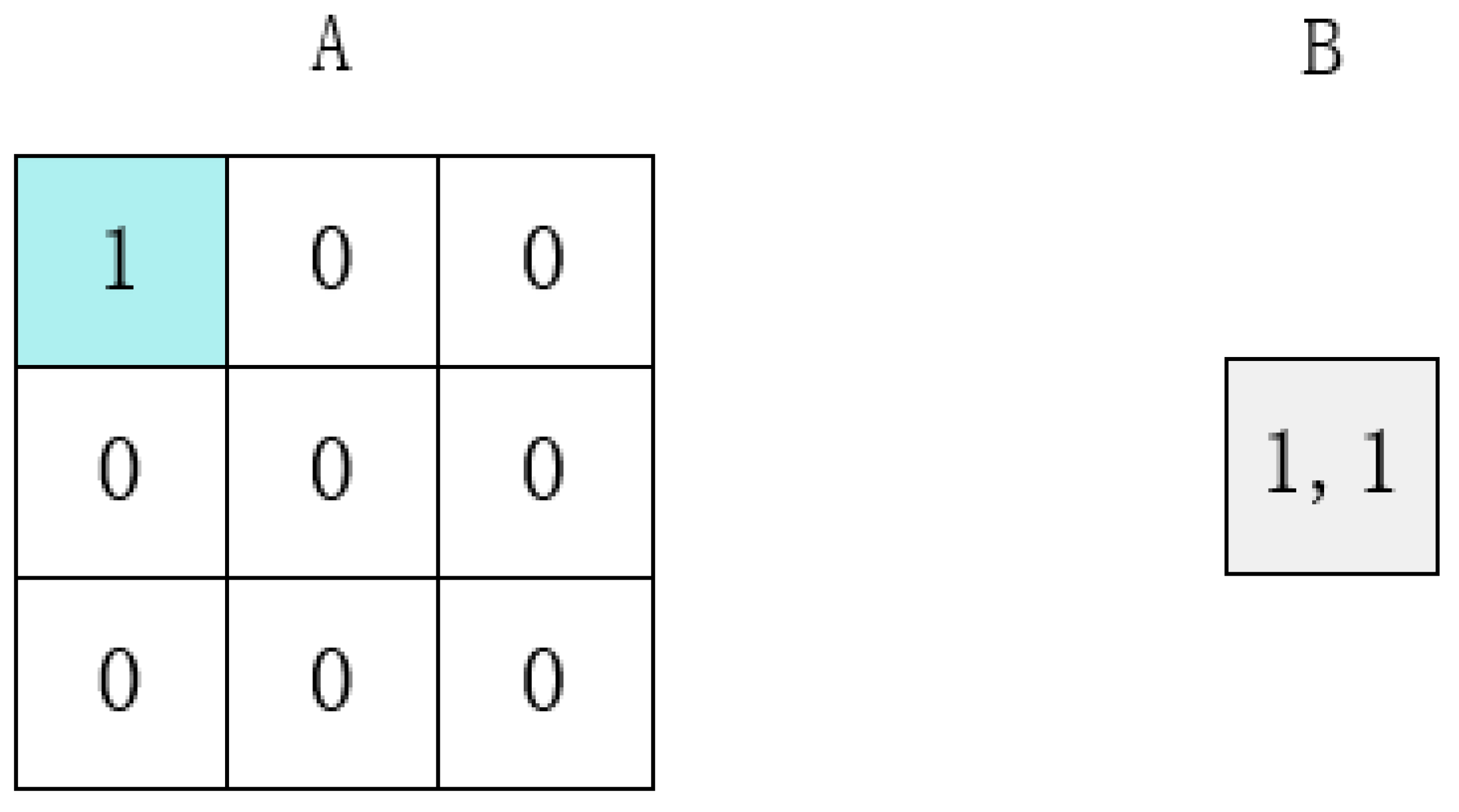
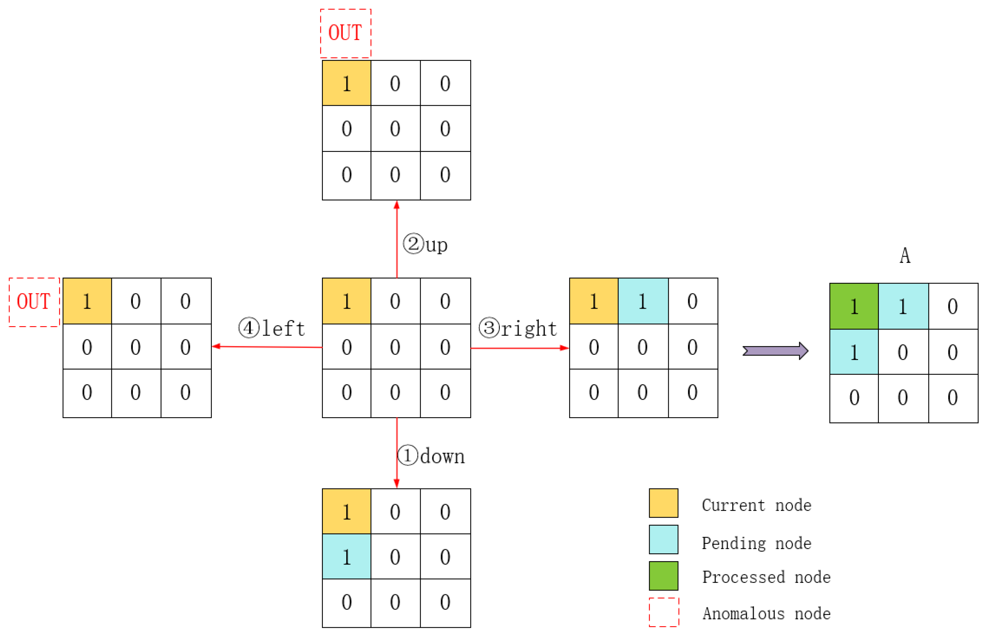
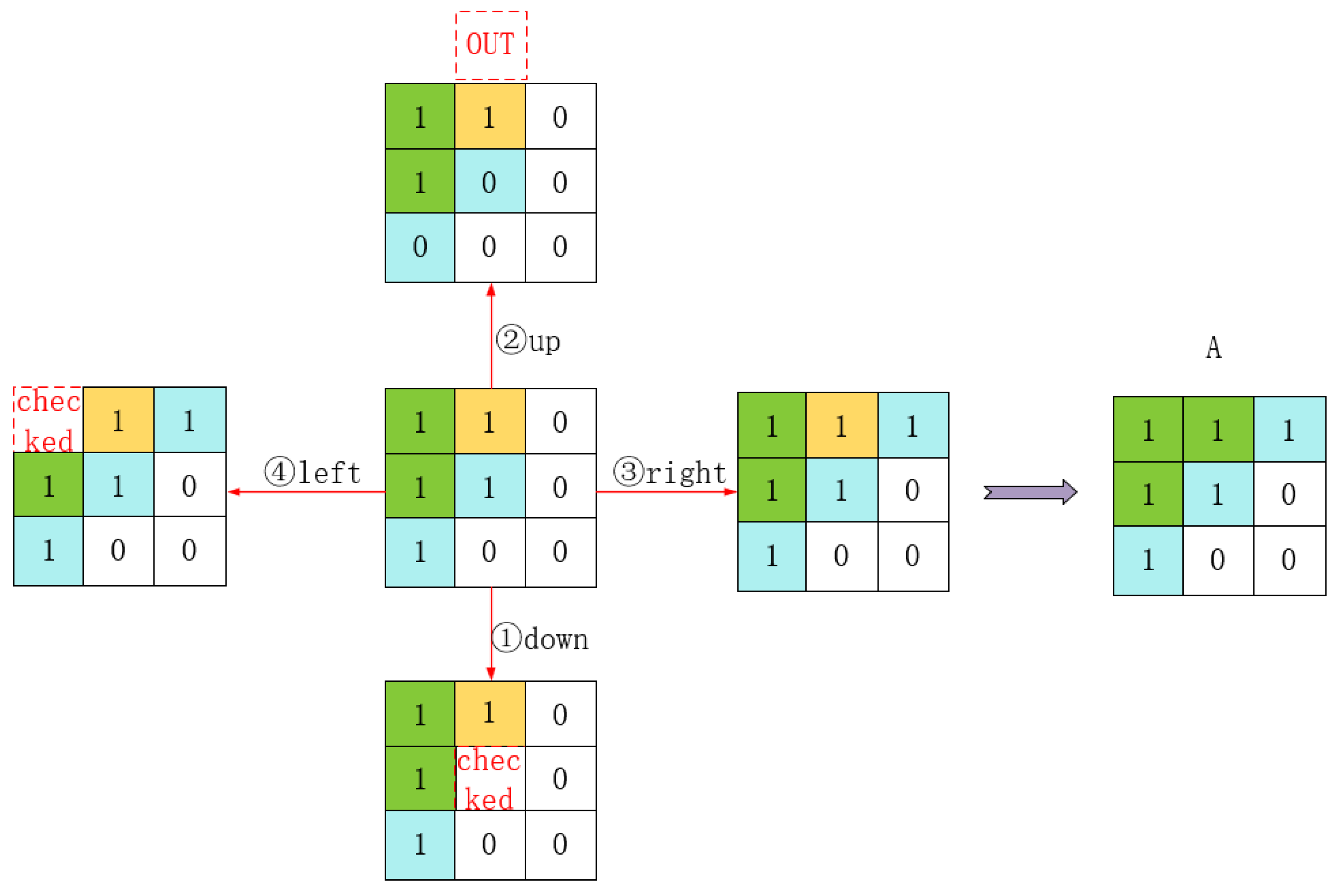
Step 2: Select the top-left corner ( 1 , 1 ) of the image matrix P as the traversal starting point. Mark this coordinate as visited and store it in the first row of matrix B. Define the four-neighborhood direction vectors: [ 1 , 0 ] (down), [ 1 , 0 ] (up), [ 0 , 1 ] (right), and [ 0 , 1 ] (left). Using a breadth-first search strategy, starting from the current coordinate, examine adjacent pixels according to the predefined direction order. For each valid and unvisited neighboring coordinate, update the access marker and append the coordinate to matrix B. Repeat this process until matrix B contains all image coordinates.
(1) Visit(1,1), mark(1,1) as visited (Figure 6).
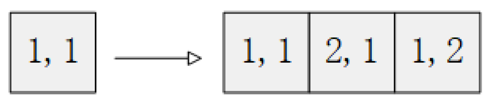
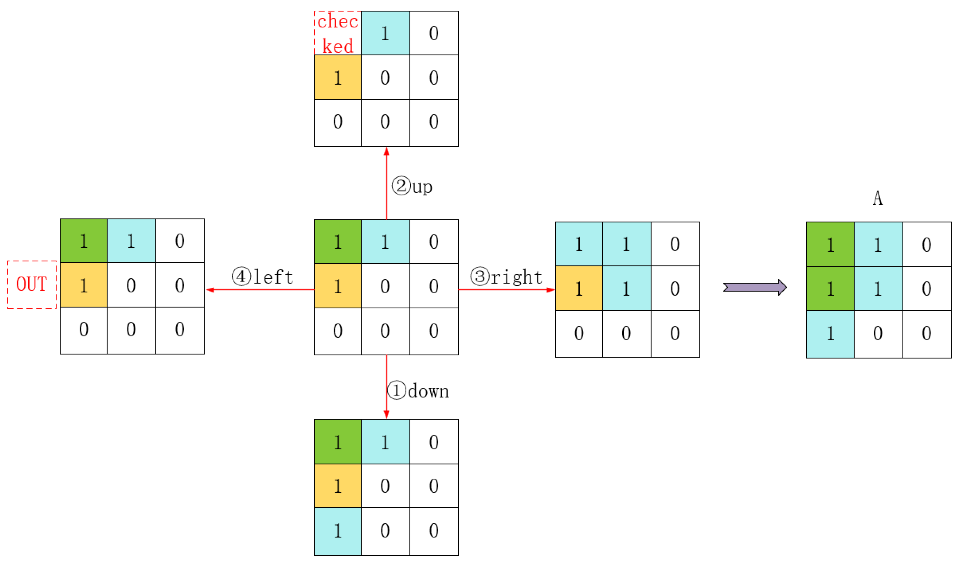
(2) Start from (1,1). Check neighbors in order: down (2,1)— valid and unvisited, add to B; up (0,1)—out of bounds; right (1,2)—valid and unvisited, add to B; left (1,0)—out of bounds (see Figure 7 and Figure 8).
(3) Start from (2,1). Check adjacent pixels. Down to (3,1)—within bounds and unvisited, add to B; up to (1,1)—already visited (skip); right to (2,2)—within bounds and unvisited, add to B; left—out of bounds (invalid) (Figure 9 and Figure 10).
(4) Start from (1,2). Check adjacent pixels. Down to (2,2)—already visited (skip); up—out of bounds (invalid); right to (1,3)—within bounds and unvisited, add to B; left to (1,1)—already visited (skip) (Figure 11 and Figure 12).
(5) Follow this procedure until all elements in A become 1, then terminate the process, obtaining the final matrices A and B (Figure 13 and Figure 14).
Step 3: Flatten the original image pixels into vector V in row-major order:
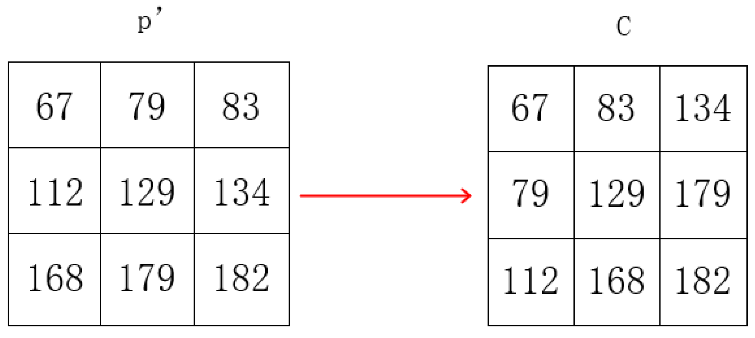
V = 67 , 79 , 83 , 112 , 129 , 134 , 168 , 179 , 182
Step 4: Using the coordinate sequence stored in matrix B, assign the i-th element of vector V to the position specified by B ( i , : ) in matrix C, i.e., C ( B ( i , 1 ) , B ( i , 2 ) ) = V ( i ) for i [ 1 , N ] . The filling process is outlined in Algorithm 2. The final encrypted image C is shown in Figure 15.
The final encrypted image C is:
Algorithm 2 Pixel Rearrangement Process
Input: Original image i m a g e [ M ] [ N ] [ C ]
Input: Coordinate sequence c o o r d _ s e q u e n c e [ M × N ] [ 2 ]
Output: Encrypted image e n c r y p t e d _ i m a g e [ M ] [ N ] [ C ]
  1:for  c h a n n e l = 1 to C do
  2:    for  i d x = 1 to M × N  do
  3:         s r c _ r o w ( i d x 1 ) / N + 1
  4:         s r c _ c o l ( i d x 1 ) mod N + 1
  5:         n e w _ r o w c o o r d _ s e q u e n c e [ i d x ] [ 1 ]
  6:         n e w _ c o l c o o r d _ s e q u e n c e [ i d x ] [ 2 ]
  7:         e n c r y p t e d _ i m a g e [ n e w _ r o w ] [ n e w _ c o l ] [ c h a n n e l ] i m a g e [ s r c _ r o w ] [ s r c _ c o l ] [ c h a n n e l ]
  8:    end for
  9:end for

4. Encryption and Decryption Algorithm

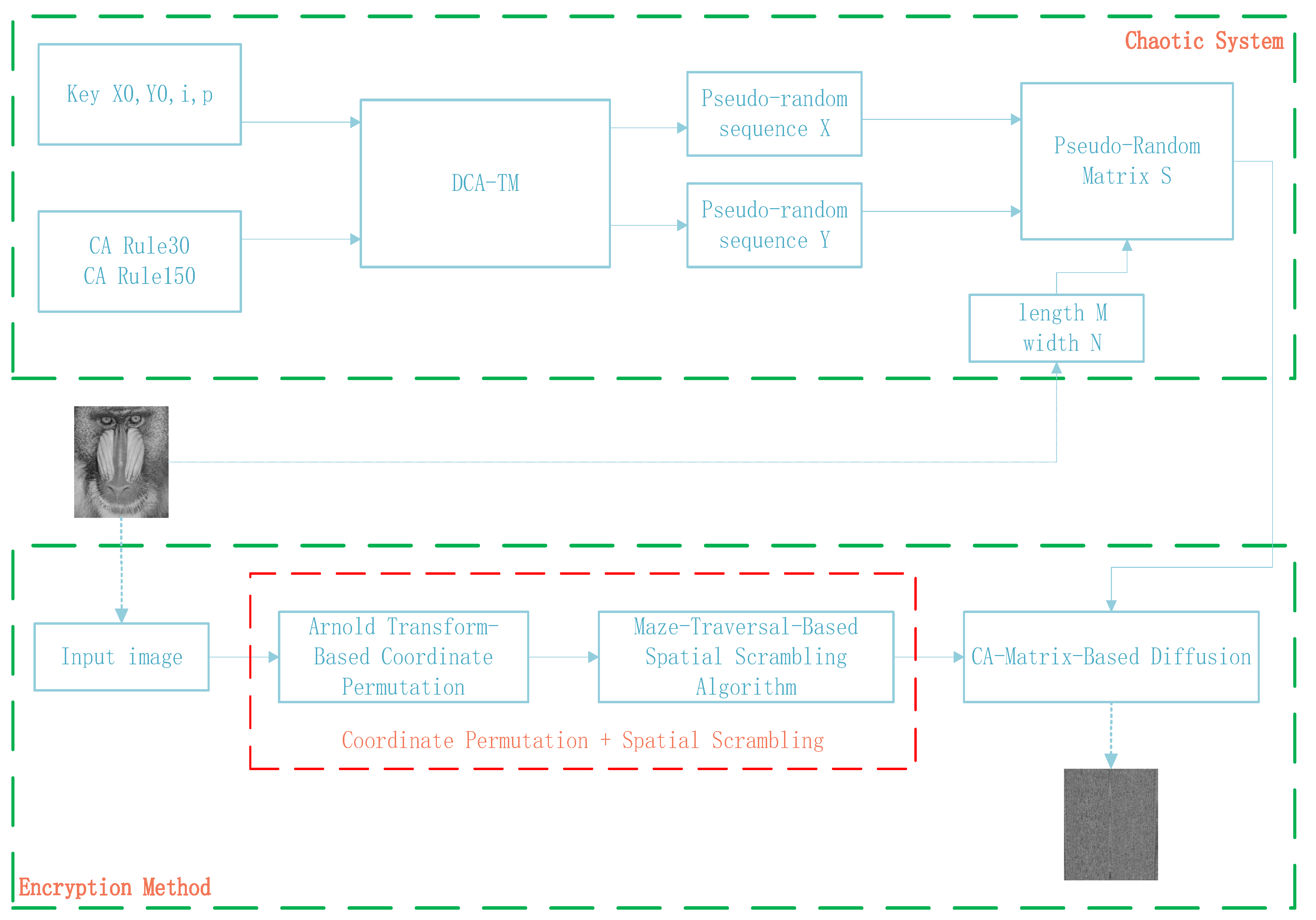
Based on the pseudo-random sequence generated by the chaotic system described above, this work abandons the traditional scrambling–diffusion encryption mechanism and adopts an encryption structure of coordinate scrambling–spatial scrambling–diffusion. Three encryption algorithms are designed: an Arnold-based coordinate scrambling method, a maze traversal-based scrambling method, and a CA matrix-based diffusion method. The flowchart of the encryption algorithm is shown in the Figure 16.

4.1. Arnold-Based Coordinate Scrambling

This work employs an Arnold transform-based scrambling method in the first step of the encryption process to perform coordinate scrambling on the original image. For each pixel in the original image, specific mathematical transformations are applied to its coordinates to disrupt the spatial structure of the image. The transformation formulas are as follows:
x ^ = ( x + b y ) mod M y ^ = ( r q x + ( 1 + b r q ) y ) mod N
where M and N are the width and height of the image, respectively, b and r are arbitrary integers, and q = N / gcd ( M , N ) , with gcd being the greatest common divisor. After coordinate scrambling, the originally meaningful image is transformed into a meaningless one, achieving preliminary information hiding.
Step 1: Let the original image size be M × N (M is the width, N is the height). Select integers b (horizontal stretching factor) and r (vertical coupling coefficient), and define the auxiliary parameter q = N / gcd ( M , N ) .
Step 2: For any pixel ( x , y ) [ 0 , M 1 ] × [ 0 , N 1 ] , its scrambled coordinates ( x ^ , y ^ ) satisfy Equation (7).
Step 3: Move the original pixel ( x , y ) to the new position ( x ^ , y ^ ) .
Invertibility proof:The transformation can be written in matrix form as
x ^ y ^ = 1 b r q 1 + b r q x y ( mod M , N )
where the modular operations are applied separately: x ^ modulo M, y ^ modulo N. The determinant of the coefficient matrix is
det = 1 · ( 1 + b r q ) b · ( r q ) = 1 + b r q b r q = 1 .
Since the determinant is 1, the matrix is invertible over the integers. The inverse transformation is given by
x y = 1 + b r q b r q 1 x ^ y ^ ( mod M , N ) .
Thus, the coordinate scrambling step is strictly bijective and fully reversible.

4.2. Spatial Scrambling via Maze Traversal

In the second step of the encryption process, this work employs a maze traversal-based spatial scrambling algorithm. This algorithm rearranges the pixel matrix of the image by simulating the process of maze traversal, thereby achieving spatial scrambling of the image.
Step 1: Initialize three matrices A, B, and S. Matrix A is used to record visited coordinates, ensuring each coordinate is accessed only once. Matrix B stores the order of the visited coordinates, serving as the basis for subsequent pixel rearrangement. Matrix S is a zero matrix with the same dimensions as the original image, used to store the encrypted pixel values.
Step 2: Starting from the top-left coordinate ( 1 , 1 ) of the image, traverse the pixel matrix in a maze-like manner using direction vectors (down, up, right, left). During traversal, record each accessed coordinate in matrix B.
Step 3: After traversal is complete, sequentially copy the pixel values from the original image to the corresponding new coordinates in matrix S according to the order recorded in matrix B, thereby achieving spatial rearrangement of the pixels.

4.3. CA Matrix-Based Diffusion

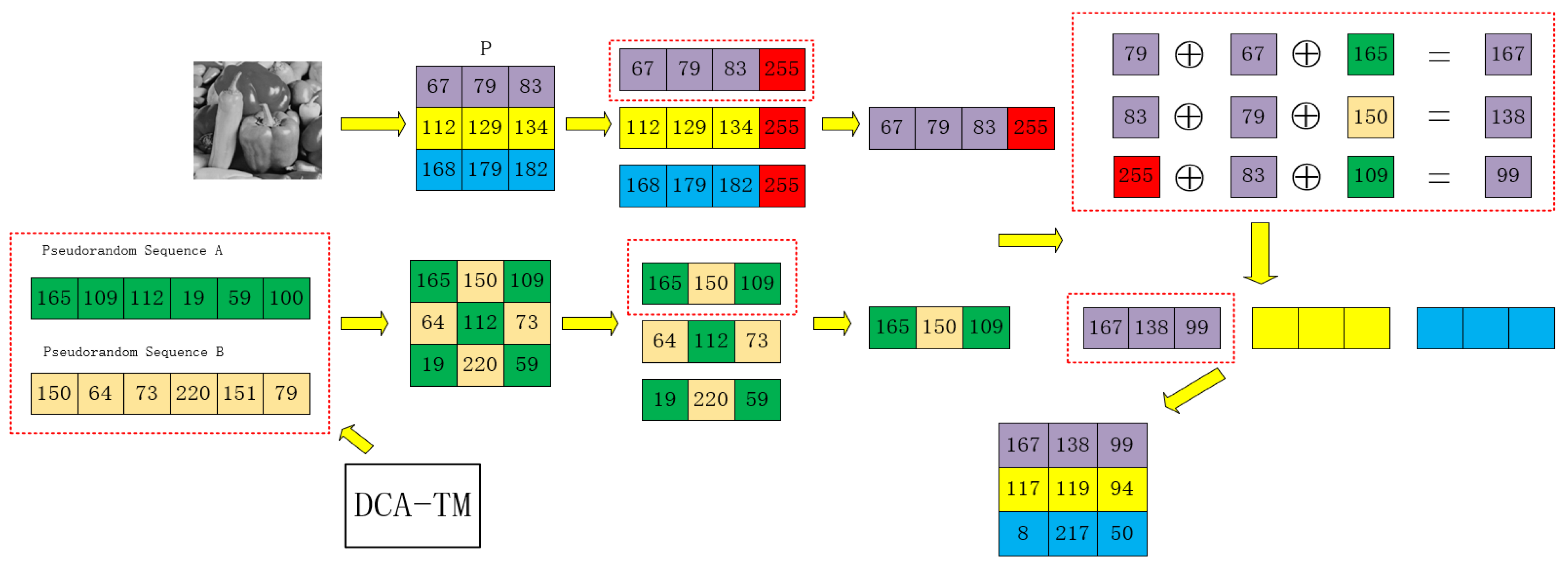
This work employs a diffusion method based on a cellular automata (CA) matrix in the third step of the encryption process. This method utilizes a pseudo-random matrix derived from a chaotic system to perform row-by-row and column-by-column diffusion processing on the pixel values of the image. Assuming the image has M rows and N columns, the specific implementation process is as follows:
Step 1: Extract pseudo-random numbers sequentially from the pseudo-random matrices A and B obtained from the chaotic system, and arrange them in row-major order to form an M × N matrix S.
Step 2: Starting from the first row, process the pixel value in the second column of the first row by performing a bitwise XOR operation with the pixel value in the first column. Then, perform another bitwise XOR operation on the result with the value at the first row and first column of matrix S. This yields a new pixel value, which is temporarily stored as the updated value for the second column of the first row (to be used in subsequent steps).
Step 3: Continue processing the pixel in the third column of the first row. Perform a bitwise XOR operation with the pixel value in the second column (i.e., the temporary value computed in the previous step, which now serves as the “new” pixel value for the second column), followed by a bitwise XOR operation with the value at the first row and second column of matrix S. Assign the resulting value to the pixel in the second column of the first row.
Step 4: Repeat this process column by column for the pixels in the first row until the pixel in the (N − 1)-th column of the first row is updated. For the pixel in the N-th column of the first row, perform a bitwise XOR operation with the constant 255 and the value at the first row and N-th column of matrix S, then assign the result to the pixel in the N-th column of the first row.
Step 5: After completing the processing of the first row, apply the same steps to the second row through the M-th row. That is, for each row, start from the second column and sequentially perform bitwise XOR operations with the pixel value from the previous column and the corresponding value in matrix S until the last pixel of the row is processed.
The diffusion flowchart is shown in Figure 17.
For clarity and to facilitate independent implementation, the complete encryption procedure is summarized in Algorithm 3. The algorithm integrates the three phases described above—coordinate permutation, maze traversal spatial scrambling, and CA matrix diffusion—into a unified pipeline. It takes the plaintext image P and the secret key K = ( x 0 , y 0 , p ) as inputs, and outputs the ciphertext image C. The corresponding decryption procedure executes the exact inverse of each phase, relying on the identical chaotic keystream regenerated from the shared secret key.
Algorithm 3 Complete Encryption Procedure
Input: Plaintext image P of size M × N , secret key K = ( x 0 , y 0 , p )
Output: Ciphertext image C of size M × N
 1:// Phase 0: Initialization
2:Generate chaotic sequences { x n } , { y n } by iterating DCA–TM (Equation (3)) with initial states ( x 0 , y 0 , p ) .
3:Discard first 10 3 iterations to eliminate transient effects.
4:Extract required parameters from chaotic sequences as needed (e.g., Arnold coefficients b , r , CA iteration count T).
5:// Phase 1: Coordinate Permutation (Arnold Transform)
6:Compute q N / gcd ( M , N ) .
7:for each pixel at coordinate ( x , y ) in P do
8:     x ^ ( x + b · y ) mod M
9:     y ^ ( r · q · x + ( 1 + b · r · q ) · y ) mod N
10:     P ( x ^ , y ^ ) P ( x , y )
11:end for
12:// Phase 2: Spatial Permutation (Maze Traversal)
13:Generate coordinate sequence B of length M × N using maze traversal (BFS on M × N grid).
14:Flatten P into vector V in row-major order.
15:for  i = 1 to M × N  do
16:     ( r o w , c o l ) B ( i )
17:     P ( r o w , c o l ) V ( i )
18:end for
19:// Phase 3: Diffusion (CA Matrix XOR)
20:Generate pseudo-random matrix S of size M × N from chaotic sequences { x n } .
21:for  i = 1 to M do
22:    for  j = 2 to N do
23:         P ( i , j ) P ( i , j ) P ( i , j 1 ) S ( i , j )
24:    end for
25:end for
26:for  j = 1 to N do
27:    for  i = 2 to M do
28:         P ( i , j ) P ( i , j ) P ( i 1 , j ) S ( i , j )
29:    end for
30:end for
31: C P  C
The decryption procedure executes the exact inverse of each phase, using the same chaotic keystream generated from the shared secret key.

5. Experimental Results and Performance Analysis

5.1. Encryption and Decryption Results

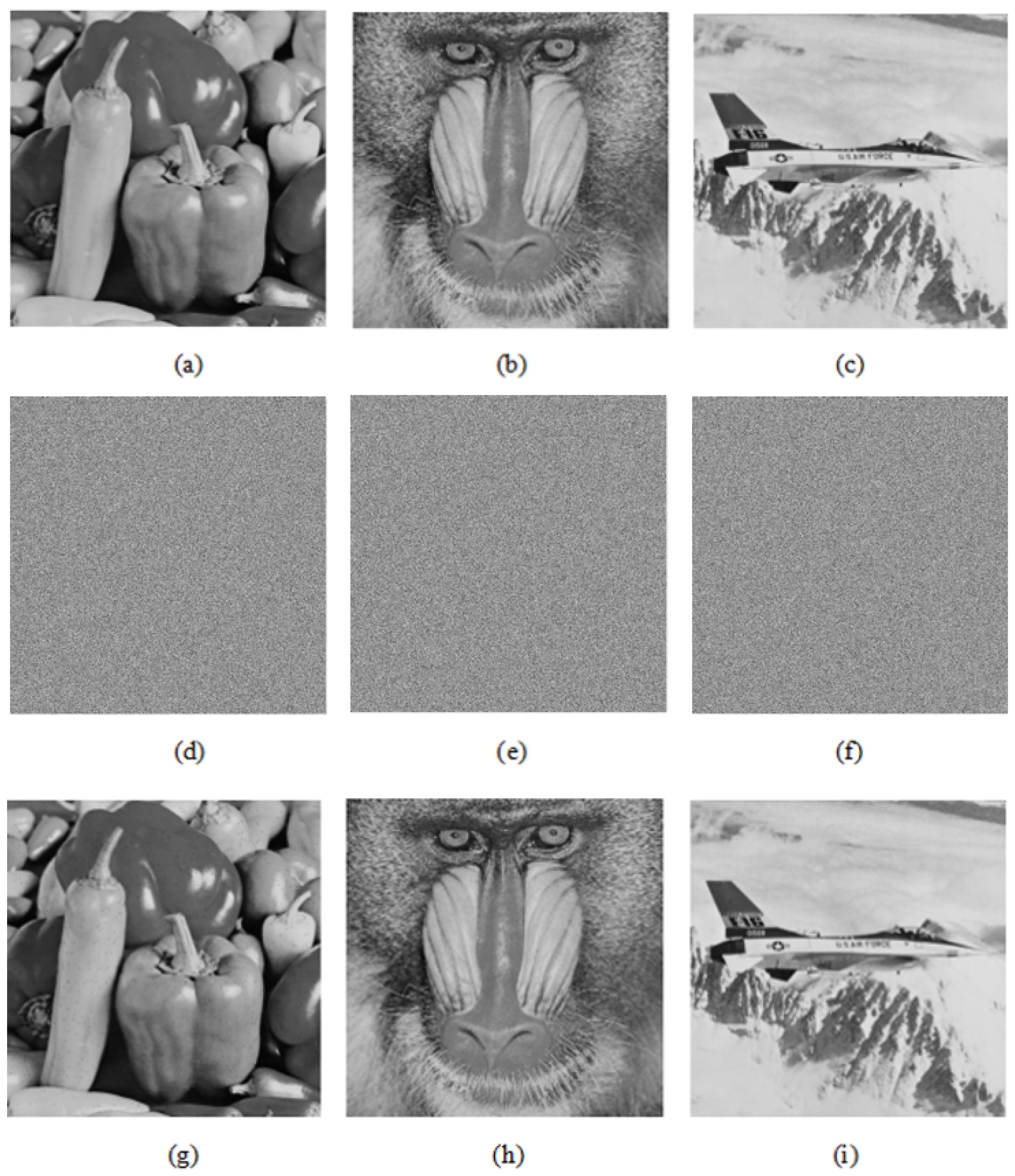
The simulation results of the encryption scheme are shown in Figure 18: (a)–(c) represent the original unencrypted images Peppers, Baboon, and Airplane; (d)–(f) are the corresponding encrypted noise-like images; (g)–(i) show the decrypted images, respectively. As can be observed, the encrypted images become completely unrecognizable noise patterns, while the decrypted images are visually indistinguishable from the original ones. Moreover, the decrypted images have essentially restored the original pixel information within numerical precision limits.

5.2. Key Space and Sensitivity Analysis

The key space, representing the total number of distinct keys that can be used in an encryption scheme, is a fundamental metric for evaluating its resistance to brute-force attacks. In the proposed encryption scheme, the total key space is determined by the combination of the sensitive parameters of the chaotic system and the initial conditions governing the cellular automata (CA). A rigorous estimation must consider the finite precision of physical implementations and the interdependence of key components.
The key space is derived from the Cartesian product of the following independent factors:
Chaotic parameter space: The system utilizes a tent map, which is highly sensitive to its initial condition x 0 and control parameter μ . In a practical digital computer environment with double-precision floating-point representation (64-bit double format according to the IEEE 754 standard) [65], the valid precision for real numbers is approximately 2 52 for the mantissa. This limits the number of distinct states that x 0 and μ can assume. However, considering the entire 64-bit representation (including sign and exponent) for key space calculation, each parameter can be considered to have 2 64 possible values. Since both x 0 and μ are used as keys, the effective key space contributed by the chaotic map is 2 64 × 2 64 = 2 128 .
CA rule-switching dynamics: The system supports k available CA rules. Importantly, the switching sequence is not an independent key but is deterministically driven by the chaotic sequences generated from the tent map. Therefore, the rule combination space does not independently multiply the total entropy. Instead, the number of possible switching sequences is inherently bounded by the number of possible chaotic sequences ( 2 128 ). The specification of the rule set (e.g., which k rules are used) can be considered part of the algorithm’s configuration. For the key space estimation, we consider the uncertainty in the switching pattern as fully embedded within the sensitivity of the initial chaotic parameters. If we were to treat the switching pattern as a separate variable (e.g., a combination of m selections from k rules), its theoretical size would be k m . However, since this pattern is purely deterministic based on x 0 and μ , it does not add extra entropy beyond the chaotic parameter space. To avoid overestimating the key space, we do not multiply the total by k m as an independent factor, but rather acknowledge that the chaotic parameters control this complexity.
Variable iteration space: The number of CA iterations T is dynamically determined by a segment of the chaotic sequence within a predefined range (e.g., T [ T min , T max ] ). This introduces additional uncertainty because the exact number of rounds is unknown to an attacker without the key. Assuming T is an integer derived from the chaotic sequence, the number of possible values it can take is ( T max T min + 1 ) . The entropy contributed by this factor is log 2 ( T max T min + 1 ) bits, resulting in a space of 2 log 2 ( T max T min + 1 ) .
Based on the above analysis, the total effective key space K is the product of the independent chaotic parameter space and the iteration space:
K = 2 128 × 2 log 2 ( T max T min + 1 ) .
In our specific implementation, we utilize two CA rules (Rule 30 and Rule 150) switched by the chaotic sequence. The iteration count T is confined to the interval [ 50 , 150 ] . Therefore, the total key space is:
K = 2 128 × 2 log 2 ( 150 50 + 1 ) = 2 128 × 2 log 2 ( 101 ) .
Since 2 6 = 64 and 2 7 = 128 , log 2 ( 101 ) 6.66 . To provide a conservative estimate in terms of bit length, we can state the key space is approximately:
K 2 128 × 2 6.66 = 2 134.66 2 135 .
This key space ( 2 135 ) is sufficiently large to resist exhaustive brute-force attacks with current computational capabilities. It is important to note that the rule-switching mechanism, while deterministic, ensures that the encryption process is highly complex and non-linear, and its full entropy is captured by the sensitivity of the initial chaotic parameters.
K e y 1 = 0.525000000000000000
K e y 2 = 0.525000000000000001
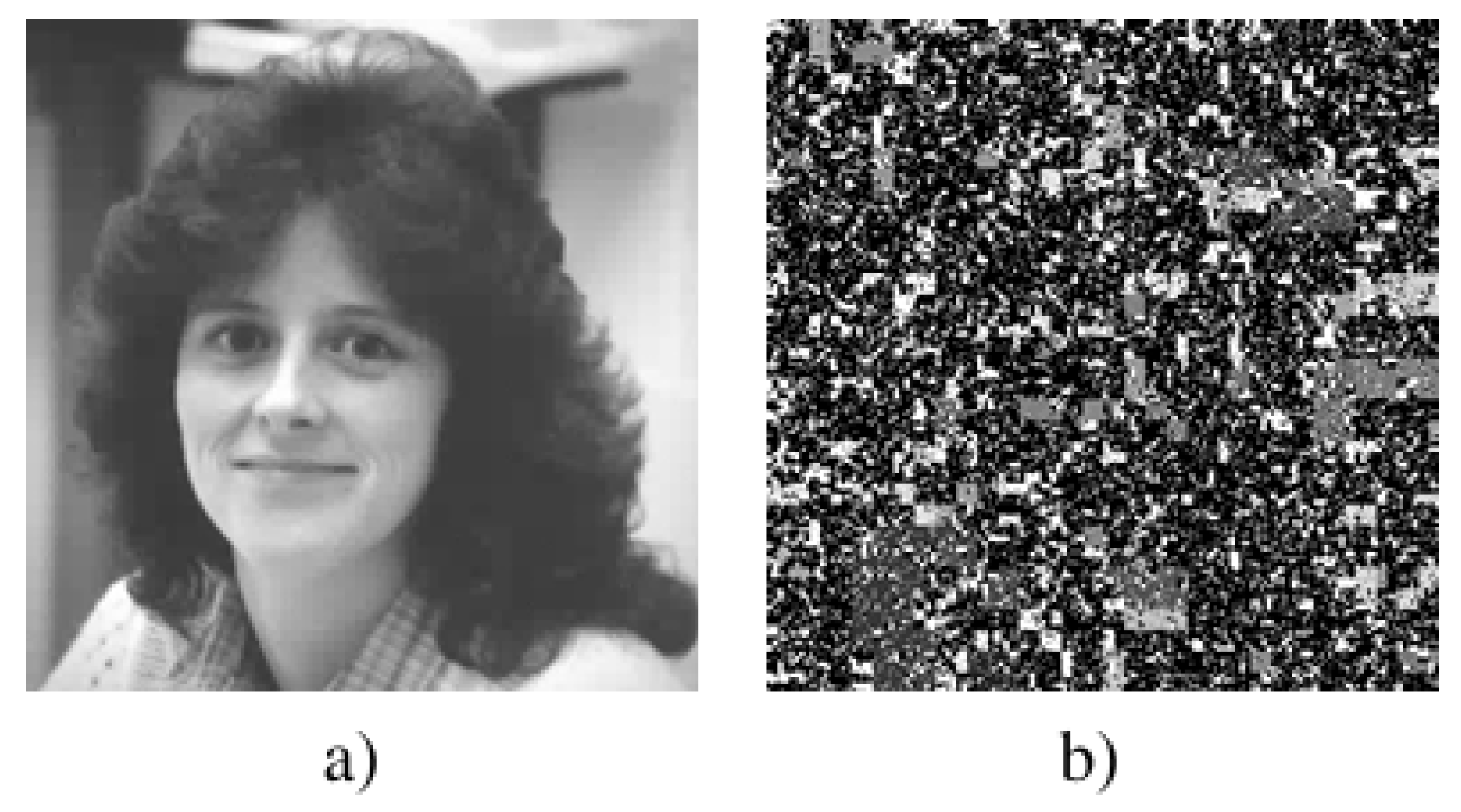
Here, Key1 is the correct key value, and Key2 is a slightly modified key. These two keys will then be used to decrypt the encrypted image. The results are shown in Figure 19: (a) shows the image decrypted with the correct key, while (b) shows the image decrypted with the slightly modified Key2. It can be seen from the figures that the image encryption algorithm proposed in this chapter is highly sensitive to the key.

5.3. Correlation Analysis

Randomly select 1000 pairs of adjacent pixels in the horizontal, vertical, and diagonal directions from the plaintext image and the target encrypted image, and calculate the correlation between adjacent pixels. The smaller this value, the better the encryption effect.
As can be seen from Table 3, the image encryption method based on chaotic systems in this example exhibits significantly lower correlation between adjacent pixels after encryption compared to other designs in the literature, with values almost approaching zero, demonstrating superior encryption performance.

5.4. Entropy Analysis

Entropy can measure the distribution of image grayscale values. The more uniform the grayscale distribution, the higher the entropy value. It serves as an indicator to evaluate the performance of image encryption—the closer this value is to 8, the better the encryption effect.
As shown in Table 4, compared with other schemes in the literature, the chaotic system-based image encryption method in this embodiment achieves an entropy value closest to 8, demonstrating its superior encryption performance.

5.5. Ability of Resisting Noise and Data Loss

Salt-and-pepper noise attack is a common form of noise interference in digital image processing. In this attack, certain pixels in the image are randomly selected and set to either the minimum or maximum pixel value, thereby introducing black and white speckles into the image.
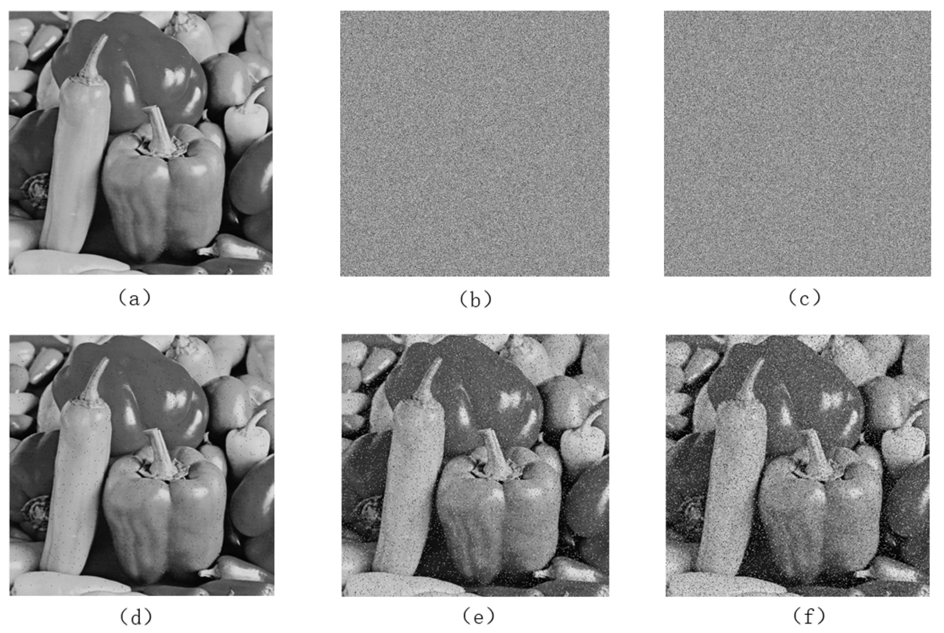
The results of salt-and-pepper noise attack are shown in Figure 20: (a) original image; (b) encrypted image with 0.05 density noise attack; (c) encrypted image with 0.1 density noise attack; (d) decrypted image of (a); (e) decrypted image of (b); (f) decrypted image of (c). As demonstrated by the noise attack results, the proposed encryption scheme can effectively reconstruct the original image information even under high-density salt-and-pepper noise interference.
Gaussian noise is introduced by adding random noise following a Gaussian distribution to the image. The noise intensity can be controlled by adjusting the standard deviation (sigma) of the Gaussian distribution—the larger the sigma value, the more severe the noise degradation in the image.
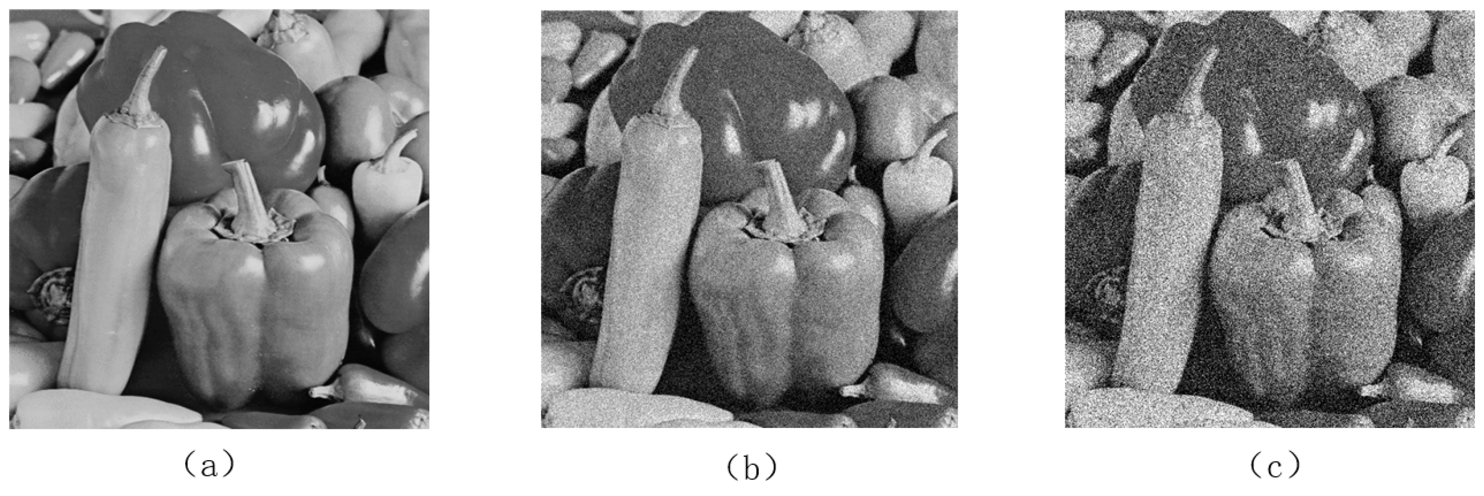
The Gaussian noise attack results are illustrated in Figure 21: (a) decrypted image of the original image; (b) decrypted image after 0.01 Gaussian noise interference on the encrypted image; (c) decrypted image after 0.05 Gaussian noise interference on the encrypted image. As evidenced by the Gaussian noise attack results, the decrypted images maintain high visual recognizability and structural integrity even under relatively strong Gaussian noise interference.
A cropping attack refers to an adversarial scenario where an attacker extracts a partial region from an encrypted image, attempting to analyze or process this cropped segment to obtain valuable information. This attack exploits potential vulnerabilities in the local region processing of image encryption algorithms. By compromising image integrity and altering pixel distribution structures, the attack impacts decryption effectiveness, leading to inter-block synchronization information loss during decryption. Consequently, the decrypted image may exhibit localized distortions or irreversible reconstruction failures.
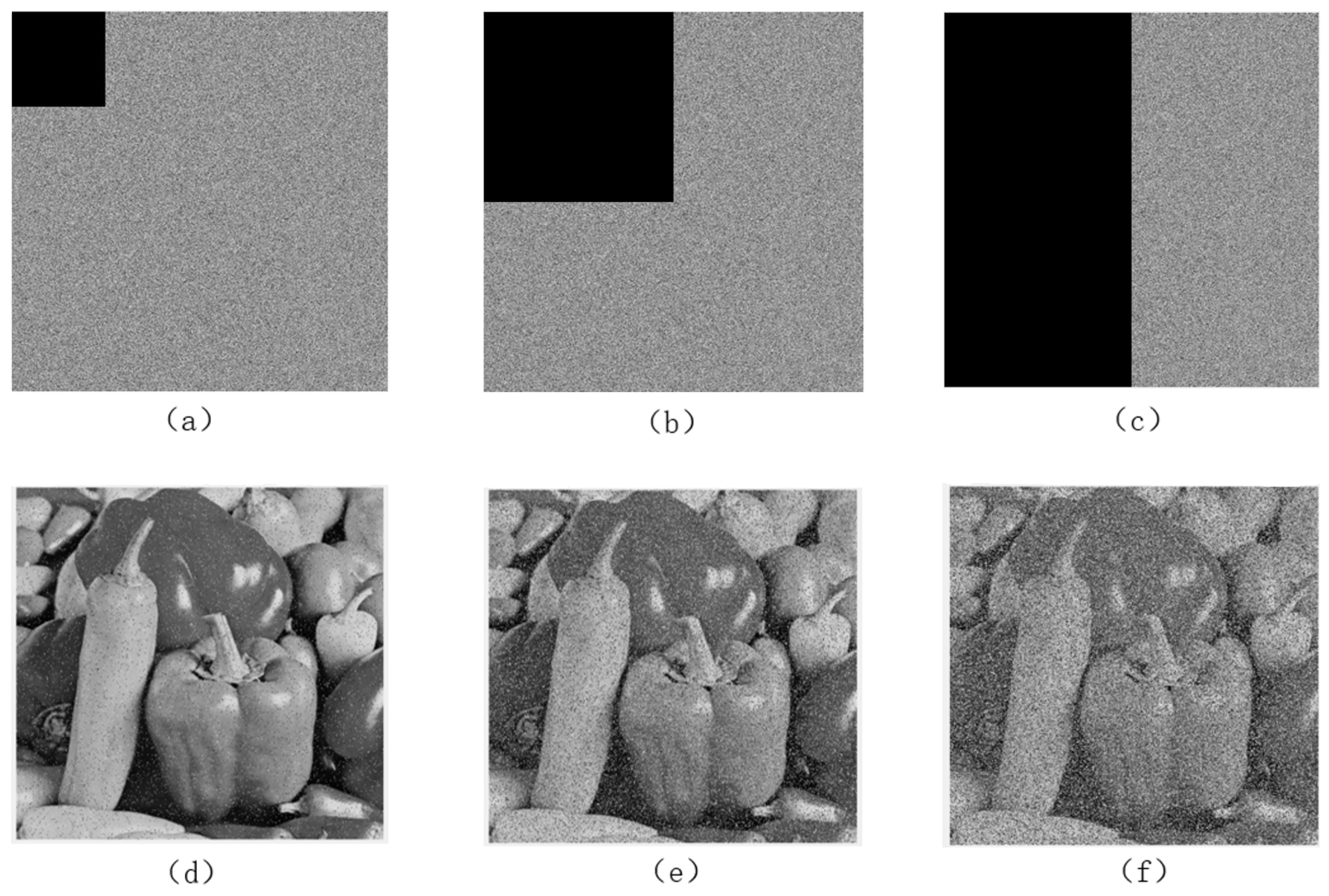
The cropping attack results are shown in Figure 22: (a) encrypted image with 1/16 area cropped; (b) encrypted image with 1/8 area cropped; (c) encrypted image with 1/4 area cropped; (d) decrypted image of (a); (e) decrypted image of (b); (f) decrypted image of (c). The results demonstrate that the decrypted images reconstructed from attacked encrypted versions exhibit neither localized distortions nor reconstruction failures. This confirms the scheme’s strong resistance against cropping attacks.
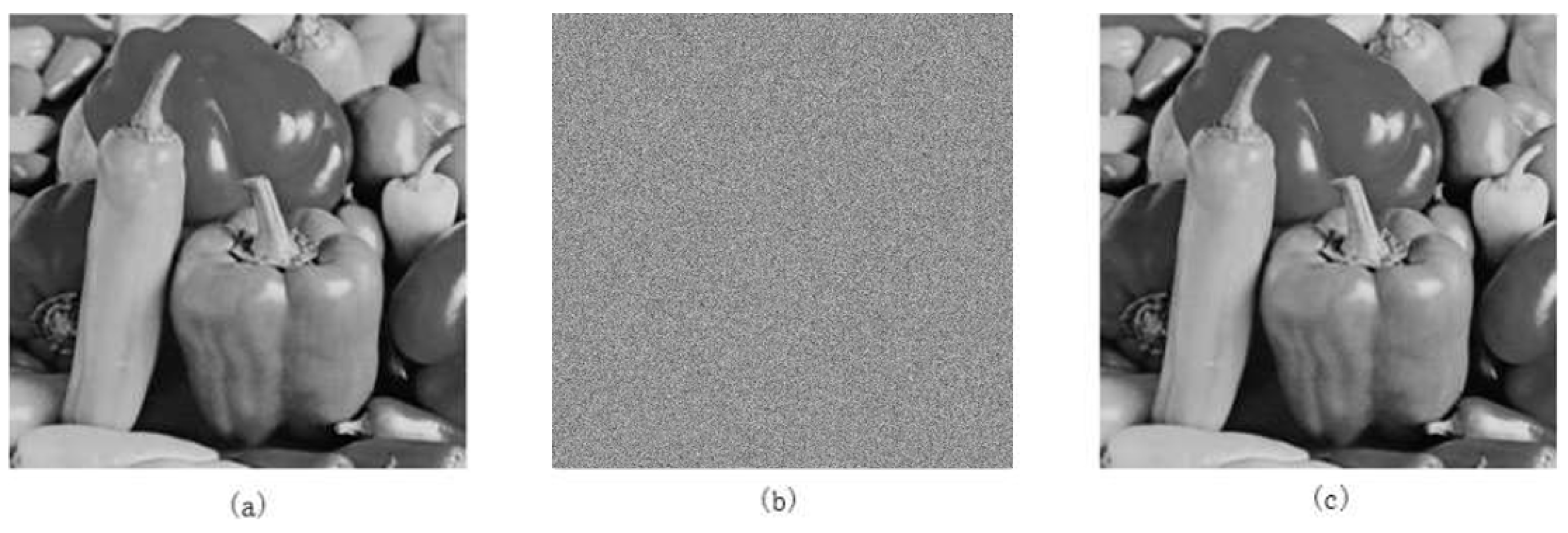
Chosen-plaintext attack (CPA) is an attack model wherein the adversary, who possesses knowledge of the encryption algorithm, can choose arbitrary plaintexts and obtain their corresponding ciphertexts. The goal of the adversary is to derive the secret key, despite having this capability. Under a chosen-plaintext attack (CPA) scenario, when fully black or fully white images are selected as the plaintext, the resulting ciphertext images exhibit the following characteristics: they appear random, their histograms remain uniform, and their information entropy is close to 8. These properties demonstrate the algorithm’s capability of withstanding chosen-plaintext attacks. The CPA results are shown in Figure 23: (a) original image; (b) the encrypted image under CPA; (c) decrypted image. The experimental results indicate that the ciphertexts of fully black and white images appear random, with uniform histograms and information entropy values of 7.99928 and 7.99940, both close to 8. These results confirm that all evaluated metrics meet the required security criteria, proving the algorithm’s resistance to CPA.
The degree of difference between two ciphertext images can be quantitatively measured using two indicators: the Number of Pixels Change Rate (NPCR) and the Unified Average Change Intensity (UACI). These two indicators are defined as the normalized L0 and L1 norm differences between the two images, respectively, with the specific calculation formulas shown in Equations (8) and (9). In these equations, C1 and C2 represent the two ciphertext images obtained by encrypting the original plaintext image and the modified plaintext image, respectively. M and N denote the dimensions of the images, and the sign(·) function returns 0 if its argument is 0, and 1 otherwise.
NPCR = i = 1 M j = 1 N | sign ( C 1 ( i , j ) C 2 ( i , j ) ) | M × N × 100 .
UACI = 1 M × N i = 1 M j = 1 N | C 1 ( i , j ) C 2 ( i , j ) | 255 × 100 .
Theoretically, the NPCR value is approximately 99.6024, and the UACI value is close to 33.4635. Table 5 presents a comparison of NPCR and UACI values for the Peppers image using different encryption methods.

5.6. Time Complexity Analysis

The time consumption of the proposed algorithm primarily appears in the following three phases:
Phase 1: Coordinate permutation (Arnold transformation). In this stage, coordinate transformation is performed for each pixel of the original image, necessitating traversal of all pixel positions. The time complexity is O ( M × N ) , where M and N are the width and height of the image, respectively.
Phase 2: Maze traversal-based spatial permutation. This stage rearranges pixel positions using a breadth-first search strategy. As described in Section 3, it requires initializing the access marker matrix A ( M × N ) and the coordinate sequence matrix B ( M N × 2 ), and performing neighborhood detection and enqueue operations for each pixel. The time complexity of a breadth-first search on a grid graph is O ( V + E ) , where V = M N is the number of nodes, and E 4 M N is the number of edges (four-neighbor connectivity). Therefore, the time complexity of this stage is O ( M N ) .
Phase 3: CA matrix-based diffusion. This stage processes the permuted image with XOR diffusion in both row-wise and column-wise directions. As described in Section 4.3, it requires traversing all pixels of the image, with each pixel undergoing two XOR operations (one with the previous pixel and one with the CA matrix value). The time complexity is O ( 2 × M × N ) = O ( M N ) .
In summary, the overall time complexity of the encryption algorithm is O ( 3 × M × N ) , which is linearly related to the total number of image pixels. It should be noted that the keystream generation phase (chaotic sequence pre-iteration) requires only constant time overhead, which is negligible.

5.7. Discussion of Experimental Findings

The experimental results presented above collectively validate the security enhancements introduced by the proposed three-phase architecture and, in particular, the dynamic CA rule-switching mechanism. The near-zero adjacent-pixel correlation coefficients (Table 3) demonstrate that the maze traversal spatial permutation effectively disrupts the strong spatial continuity inherent in natural images, while the XOR-chain diffusion further decorrelates neighboring pixels by propagating modifications across both rows and columns. The information entropy values exceeding 7.9997 (Table 4) confirm that the DCA–TM keystream possesses sufficient randomness to flatten the grayscale histogram completely; unlike static CA configurations, the deterministic yet chaotic alternation between Rule 30 and Rule 150 prevents the emergence of any recurring statistical patterns in the ciphertext. Furthermore, the retained visual recognizability under high-density noise and substantial cropping (Figure 20, Figure 21 and Figure 22) is a direct consequence of the global dispersion property conferred by the maze traversal: each plaintext pixel contributes to multiple spatially distant ciphertext positions, so that localized corruption is effectively averaged out during decryption. Finally, the NPCR and UACI metrics (Table 5) quantitatively validate the strong plaintext sensitivity of the scheme, which arises from the CA diffusion phase where a single-pixel alteration cascades through the entire image via the XOR chain, producing the avalanche effect characteristic of a secure cryptosystem. In summary, the dynamic integration of CA rule switching with the tent map not only expands the key space but also enhances diffusion uniformity and robustness against statistical and physical attacks, thereby accounting for the superior performance metrics observed across all the evaluations.

6. Conclusions

This study addresses the inherent limitations of conventional chaotic encryption methods—including periodicity, restricted key space, and insufficient attack resistance—by proposing an image encryption algorithm that integrates cellular automata with a tent map. The algorithm adopts a three-layer encryption architecture consisting of coordinate permutation, spatial permutation, and diffusion, enhancing both security and robustness through multi-stage processing.
By nonlinearly coupling dynamic cellular automaton rule switching with an improved logistic map, the proposed system achieves a 47.6% increase in the maximum Lyapunov exponent relative to the traditional tent map. The integration of dynamic rule switching and parameter sensitivity expands the theoretical key space to approximately 2 135 , providing a foundation for resistance against brute-force attacks. At the application level, the study makes two primary technical contributions. First, a dual-layer permutation mechanism is established by combining Arnold’s cat map with a maze traversal-based spatial scrambling algorithm: the former disrupts spatial structure through reversible coordinate transformation, while the latter performs a secondary global rearrangement of pixel positions via graph traversal. This strategy reduces the adjacent-pixel correlation coefficient in the encrypted image to below 0.0032 and increases the information entropy to 7.9993. Second, a dynamic rule diffusion strategy is introduced, wherein chaotic sequences govern the real-time selection of cellular automaton rules to perform nonlinear mixing of permuted pixel values. This approach not only diffuses minor pixel differences across the entire ciphertext image but also enhances robustness against noise and cropping attacks. Under 0.1-density salt-and-pepper noise and cropping of up to one-quarter of the image area, the decrypted images retain the main visual information.
Despite these advances, certain limitations remain. The current deterministic cellular automaton rule-switching mechanism could benefit from a stochastic stability analysis. Future work will incorporate modeling of rule transitions using Markov processes or stochastic differential equations and establish Lyapunov-based mean-square stability conditions, thereby providing probabilistic security guarantees and strengthening theoretical resistance to statistical cryptanalysis. To further improve the rigor and reproducibility of the evaluation framework, subsequent research will adopt standardized taxonomies and testing protocols for chaotic encryption. These will include systematic digital-chaos degradation analysis, extended security metrics, and cross-platform benchmarking, thereby enhancing the methodological completeness of the security assessment [77].

Author Contributions

Y.H.: Conceptualization, Methodology, Software, Validation, Investigation, Data Curation, Writing—Original Draft Preparation, Writing—Review and Editing, Visualization; Z.Z.: Conceptualization, Methodology, Software, Validation, Resources, Data Curation, Writing—Original Draft Preparation, Writing—Review and Editing, Project Administration, Funding Acquisition; D.L.: Formal Analysis; F.Y.: Formal Analysis, Funding Acquisition; J.J.: Validation. All authors have read and agreed to the published version of the manuscript.

Funding

This research received no external funding.

Institutional Review Board Statement

Not applicable.

Informed Consent Statement

Not applicable.

Data Availability Statement

The data that support the findings of this study are available from the corresponding author upon reasonable request.

Conflicts of Interest

The authors declare no conflicts of interest.

References

  1. Hu, J.; Shen, H.; Huang, J.; Sherratt, R.S.; Wang, J. A High-Performance Sketch with Dynamic Memory Allocation for Priority-Oriented Data Stream Processing. IEEE Trans. Comput. 2026, 75, 720–733. [Google Scholar] [CrossRef]
  2. Xu, L.; Wang, X. RegCGAN: Resampling with Regularized CGAN for Imbalanced Big Data Problem. Axioms 2025, 14, 485. [Google Scholar] [CrossRef]
  3. Hu, J.; Xu, X.; Wang, H.; Chen, X.; Wang, J.; Chen, K. DSA: Efficient Data-Plane Memory Scheduler for In-Network Aggregation to Accelerate Distributed Training. IEEE Trans. Netw. 2026, 34, 753–766. [Google Scholar] [CrossRef]
  4. Sun, J.; Li, X.; Sun, Y.; Xiong, Z.; He, J. An artificial synapse capable of regulating signal transmission speed in a neuromorphic network. Chin. Phys. B 2026, 35, 010501. [Google Scholar] [CrossRef]
  5. Xiao, P.; Ma, M.; Jiang, H.; Huan, Z.; Du, S.; Hong, Q. Analog Solver Design of LU Decomposition Algorithm for Accelerating Public Color Watermarking. IEEE Trans. Ind. Inform. 2025, 22, 969–980. [Google Scholar] [CrossRef]
  6. Sun, J.; Sun, J.; Li, X.; Sun, Y.; Hong, Q.; Wang, C. A Review of Recent Developments in Neuromorphic Computing Based on Emerging Memory Devices: J. Sun et al. Nonlinear Dyn. 2025, 113, 33035–33061. [Google Scholar] [CrossRef]
  7. Deng, Q.; Wang, C.; Sun, Y.; Cong, X.; Lin, H.; Deng, Z. Memristor-Based Brain Emotional Learning Neural Network with Attention Mechanism and Its Application. IEEE Trans. Comput.-Aided Des. Integr. Circuits Syst. 2025, 44, 4701–4713. [Google Scholar] [CrossRef]
  8. Zhu, C.; Jin, J.; Li, Z.; Ma, J.; Liu, C. Predefined-time multi-robot formation control: Based on the event-triggered ZNN models. Neurocomputing 2025, 669, 132478. [Google Scholar] [CrossRef]
  9. Yu, F.; Kong, X.; Yao, W.; Zhang, J.; Cai, S.; Lin, H.; Jin, J. Dynamics Analysis, Synchronization and FPGA Implementation of Multi-Scroll Hopfield Neural Networks with Non-Polynomial Memristor. Chaos Solitons Fractals 2024, 179, 114440. [Google Scholar] [CrossRef]
  10. Hu, J.; Huang, J.; Li, Z.; Li, Y.; Rao, S.; Jiang, W.; Chen, K.; Wang, J.; He, T. Proactive Transport with High Link Utilization Using Opportunistic Packets in Cloud Data Centers. IEEE Trans. Mob. Comput. 2025, 24, 9774–9790. [Google Scholar] [CrossRef]
  11. Hu, J.; He, Y.; Luo, W.; Huang, J.; Wang, J. Enhancing Load Balancing with In-Network Recirculation to Prevent Packet Reordering in Lossless Data Centers. IEEE/ACM Trans. Netw. 2024, 32, 4114–4127. [Google Scholar] [CrossRef]
  12. Hu, J.; Zeng, C.; Wang, Z.; Zhang, J.; Guo, K.; Xu, H.; Huang, J.; Chen, K. Load Balancing with Multi-Level Signals for Lossless Datacenter Networks. IEEE/ACM Trans. Netw. 2024, 32, 2736–2748. [Google Scholar] [CrossRef]
  13. Deng, Q.; Wang, C.; Yang, G. Discrete memristor-based complex-valued chaotic system dynamic analysis and its application in dual-image encryption. Acta Phys. Sin. 2026, 75, 010003. [Google Scholar] [CrossRef]
  14. Feng, W.; Tang, Z.; Zhao, X.; Qin, Z.; Chen, Y.; Cai, B.; Zhu, Z.; Wen, H.; Ye, C. State-Dependent Variable Fractional-Order Hyperchaotic Dynamics in a Coupled Quadratic Map: A Novel System for High-Performance Image Protection. Fractal Fract. 2025, 9, 792. [Google Scholar] [CrossRef]
  15. He, T.; Yu, F.; Lin, Y.; He, S.; Yao, W.; Cai, S.; Jin, J. Multi-scroll hopfield neural network excited by memristive self-synapses and its application in image encryption. Chin. Phys. B 2025, 34, 120506. [Google Scholar] [CrossRef]
  16. Jin, J.; Wu, M.; Ouyang, A.; Li, K.; Chen, C. A novel dynamic hill cipher and its applications on medical IoT. IEEE Internet Things J. 2025, 12, 14297–14308. [Google Scholar] [CrossRef]
  17. Huang, Y.; Huang, H.; Huang, Y.; Wang, Y.; Yu, F.; Yu, B. Asymptotic Shape Synchronization in Three-Dimensional Chaotic Systems and Its Application in Color Image Encryption. Chaos Solitons Fractals 2024, 184, 114945. [Google Scholar] [CrossRef]
  18. Nulhakim, I.D.; Hadiana, A.I.; Melina. Digital Image Security with AES and Blowfish Double Encryption. Int. J. Quant. Res. Model. 2025, 6, 364–376. [Google Scholar] [CrossRef]
  19. Zhu, J.; Jin, J.; Chen, C.; Wu, L.; Lu, M.; Ouyang, A. A New-Type Zeroing Neural Network Model and Its Application in Dynamic Cryptography. IEEE Trans. Emerg. Top. Comput. Intell. 2025, 9, 176–191. [Google Scholar] [CrossRef]
  20. Gao, S.; Ho-Ching Iu, H.; Erkan, U.; Simsek, C.; Toktas, A.; Cao, Y.; Wu, R.; Mou, J.; Li, Q.; Wang, C. A 3D Memristive Cubic Map with Dual Discrete Memristors: Design, Implementation, and Application in Image Encryption. IEEE Trans. Circuits Syst. Video Technol. 2025, 35, 7706–7718. [Google Scholar] [CrossRef]
  21. Zhang, S.; He, D.; Li, Y.; Lu, D.; Li, C. Dual Memristor-Coupled Hopfield Neural Network with Any Multi-Scroll Amplitude Control and Its Application for Medical Image Classification. IEEE Trans. Autom. Sci. Eng. 2025, 22, 17828–17840. [Google Scholar] [CrossRef]
  22. Feng, W.; Tang, Z.; Zhao, X.; Qin, Z.; Chen, Y.; Cai, B.; Zhu, Z.; Qian, K.; Wen, H. Two-Dimensional Coupling-Enhanced Cubic Hyperchaotic Map with Exponential Parameters: Construction, Analysis, and Application in Hierarchical Significance-Aware Multi-Image Encryption. Axioms 2025, 14, 901. [Google Scholar] [CrossRef]
  23. Gao, S.; Zhang, Z.; Iu, H.H.C.; Ding, S.; Mou, J.; Erkan, U.; Toktas, A.; Li, Q.; Wang, C.; Cao, Y. A Parallel Color Image Encryption Algorithm Based on a 2-D Logistic-Rulkov Neuron Map. IEEE Internet Things J. 2025, 12, 18115–18124. [Google Scholar] [CrossRef]
  24. Ma, M.; Yuan, Z.; Kalsoom, U.; Deng, W.; He, S. Dynamical behavior of ring-star neural networks with small-world characteristics. Chin. Phys. B 2025, 34, 100502. [Google Scholar] [CrossRef]
  25. Yao, W.; Wang, Y.; Xiong, L.; Xiao, J.; Zhang, S.; Sun, Y. Dynamics of asteroidal Hopfield neural network under electromagnetic radiation and its application in the mechanical optimization design: W. Yao et al. Nonlinear Dyn. 2025, 113, 35237–35254. [Google Scholar] [CrossRef]
  26. Lorenz, E.N. Deterministic Nonperiodic Flow. J. Atmos. Sci. 1963, 20, 130–141. [Google Scholar] [CrossRef]
  27. Jin, J.; Chen, W.; Ouyang, A.; Yu, F.; Liu, H. A time-varying fuzzy parameter zeroing neural network for the synchronization of chaotic systems. IEEE Trans. Emerg. Top. Comput. Intell. 2023, 8, 364–376. [Google Scholar] [CrossRef]
  28. Luo, D.; Wang, C.; Liang, J.; Deng, Q. Memristor coupled fractional-order Hopfield neural network composed by heterogeneous neurons and its FPGA implementation. Nonlinear Dyn. 2025, 113, 29983–29998. [Google Scholar] [CrossRef]
  29. Yu, X.; Huang, L.; Bao, H.; Bao, B. A Morris-Lecar model with novel fast-slow structure and its FPGA implementation. Sci. China Technol. Sci. 2025, 68, 1520405. [Google Scholar] [CrossRef]
  30. Bao, H.; Fan, J.; Hua, Z.; Xu, Q.; Bao, B. Discrete Memristive Hopfield Neural Network and Application in Memristor-State-Based Encryption. IEEE Internet Things J. 2025, 12, 31843–31855. [Google Scholar] [CrossRef]
  31. Souza, C.E.C.; Moreno, D.; Sousa, M.H.S.; Chaves, D.P.B.; Pimentel, C. High-Throughput Pseudo-Random Number Generators Over Discrete Chaos. IEEE Trans. Circuits Syst. II Express Briefs 2025, 72, 1303–1307. [Google Scholar] [CrossRef]
  32. Yu, F.; He, S.; Yao, W.; Cai, S.; Xu, Q. Bursting Firings in Memristive Hopfield Neural Network with Image Encryption and Hardware Implementation. IEEE Trans. Comput.-Aided Des. Integr. Circuits Syst. 2025, 44, 4564–4576. [Google Scholar] [CrossRef]
  33. Yang, G.; Wang, C.; Sun, Y.; Deng, Q. Delayed discrete memristive ring neural network and application in pseudorandom number generator. IEEE Internet Things J. 2025, 13, 11425–11435. [Google Scholar] [CrossRef]
  34. Yu, F.; Wang, X.; Guo, R.; Ying, Z.; Cai, S.; Jin, J. Dynamical analysis, hardware implementation, and image encryption application of new 4D discrete hyperchaotic maps based on parallel and cascade memristors. Integration 2025, 104, 102475. [Google Scholar] [CrossRef]
  35. Yang, G.; Wang, C.; Sun, Y.; Deng, Q. A Class of Discrete Memristive Hyperchaotic Maps with Multicavity Multistructure Attractors and Its Application in Secure Communication. IEEE Trans. Ind. Inform. 2026, 22, 1–12. [Google Scholar] [CrossRef]
  36. Yu, F.; He, T.; He, S.; Tan, B.; Shi, C.; Lin, H. Influence of memristive activated gradient on chaotic dynamics in discrete neural networks. Int. J. Bifurc. Chaos 2025, 35, 2550146. [Google Scholar] [CrossRef]
  37. Yang, G.; Wang, C.; Sun, Y.; Deng, Q. A discrete memristive heterogeneous Hopfield neural network with multi-penguin-like/silkworm-like attractors and its application in secure communication. Nonlinear Dyn. 2026, 114, 259. [Google Scholar] [CrossRef]
  38. Yu, F.; Wang, X.; Guo, R.; Ying, Z.; He, Y.; Zou, Q. Discrete neuron models and memristive neural network mapping: A comprehensive review. Chin. Phys. B 2025, 34, 120501. [Google Scholar] [CrossRef]
  39. Yang, G.; Wang, C.; Sun, Y.; Deng, Q. A Discrete Memristive Hopfield Neural Network with Grid Multi-structure/scroll-like Attractors. IEEE Trans. Comput.-Aided Des. Integr. Circuits Syst. 2026, 45, 1. [Google Scholar] [CrossRef]
  40. Alvarez, G.; Li, S. Some Basic Cryptographic Requirements for Chaos-Based Cryptosystems. Int. J. Bifurc. Chaos 2006, 16, 2129–2151. [Google Scholar] [CrossRef]
  41. Matthews, R. On the Derivation of a Chaotic Encryption Algorithm. Cryptologia 2006, 13, 29–42. [Google Scholar] [CrossRef]
  42. Huang, X.; Li, C.; Zhang, S.; Liu, W. A New Image Encryption Algorithm Based on High-Dimensional Chaotic System. Nonlinear Dyn. 2021, 104, 563–576. [Google Scholar]
  43. Tutueva, A.V.; Nepomuceno, E.G.; Karimov, A.I.; Andreev, V.S.; Butusov, D.N. Adaptive Chaotic Maps and Their Application to Pseudo-Random Numbers Generation. Chaos Solitons Fractals 2020, 133, 109615. [Google Scholar] [CrossRef]
  44. Zarebnia, M.; Pakmanesh, H.; Parvaz, R. A Fast Multiple-Image Encryption Algorithm Based on Hybrid Chaotic Systems for Grayscale Images. Optik 2019, 179, 761–773. [Google Scholar] [CrossRef]
  45. Fridrich, J. Symmetric Ciphers Based on Two-Dimensional Chaotic Maps. Int. J. Bifurc. Chaos 1998, 8, 1259–1284. [Google Scholar] [CrossRef]
  46. Zhang, H.; Feng, X.; Sun, J.; Yan, P. Chaotic Image Security Techniques and Developments: A Review. Mathematics 2025, 13, 1976. [Google Scholar] [CrossRef]
  47. Li, P.; Wang, K.; Gao, S.; Xu, X.; Mou, J. Encryption scheme for multi-image based on combination of multiple chaotic maps and iterative variation of confusion keystream and mixed diffusion expression. J. King Saud Univ. Comput. Inf. Sci. 2025, 37, 278. [Google Scholar] [CrossRef]
  48. Qian, Y.; Zheng, J.; Hu, H. Dynamic time-delay perturbation: A strategy for enhancing chaotic system performance and its applications. Nonlinear Dyn. 2025, 113, 4815–4837. [Google Scholar] [CrossRef]
  49. Wolfram, S. Random Sequence Generation by Cellular Automata. Adv. Appl. Math. 1986, 7, 123–169. [Google Scholar] [CrossRef]
  50. Nandi, S.; Kar, B.K.; Pal Chaudhuri, P. Theory and Applications of Cellular Automata in Cryptography. IEEE Trans. Comput. 1994, 43, 1346–1357. [Google Scholar] [CrossRef]
  51. Chen, W.; Zhou, X.; Li, M.; Hu, M. Image Encryption Algorithm Based on Optical Chaos and Elliptic Curve. Eur. Phys. J. D 2023, 77, 197. [Google Scholar] [CrossRef]
  52. Wang, M.; Wang, X.; Wang, C.; Zhou, S.; Xia, Z.; Li, Q. Color Image Encryption Based on 2D Enhanced Hyperchaotic Logistic-Sine Map and Two-Way Josephus Traversing. Digit. Signal Process. 2023, 132, 103818. [Google Scholar] [CrossRef]
  53. Wang, Y.; Zhao, Y.; Zhou, Q.; Lin, Z. Image Encryption Using Partitioned Cellular Automata. Neurocomputing 2018, 275, 1318–1332. [Google Scholar] [CrossRef]
  54. Niyat, A.Y.; Moattar, M.H.; Torshiz, M.N. Color Image Encryption Based on Hybrid Hyper-Chaotic System and Cellular Automata. Opt. Lasers Eng. 2017, 90, 225–237. [Google Scholar] [CrossRef]
  55. Yang, Y.G.; Tian, J.; Lei, H.; Zhou, Y.H.; Shi, W.M. Novel Quantum Image Encryption Using One-Dimensional Quantum Cellular Automata. Inf. Sci. 2016, 345, 257–270. [Google Scholar] [CrossRef]
  56. Aydin, Y.; Garipcan, A.M.; Özkaynak, F. A novel secure S-box design methodology based on FPGA and SHA-256 hash algorithm for block cipher algorithms. Arab. J. Sci. Eng. 2025, 50, 1247–1260. [Google Scholar] [CrossRef]
  57. Boobalan, S.; Gurunathan Arthanari, S.K. Lorenz and Chua Chaotic Key-Based Dynamic Substitution Box for Efficient Image Encryption. Symmetry 2025, 17, 1296. [Google Scholar] [CrossRef]
  58. Kadhim, Q.; Al-Jawher, W.A.M. A new multiple-chaos image encryption algorithm based on block compressive sensing, swin transformer, and wild horse optimization. Multidiscip. Sci. J. 2025, 7, 2025012. [Google Scholar] [CrossRef]
  59. Kolivand, H.; Hamood, S.F.; Asadianfam, S.; Mohd Rahim, M.S.; Hurst, W. Image encryption framework based on multi-chaotic maps and equal pixel values quantization. Multimed. Tools Appl. 2025, 84, 17769–17804. [Google Scholar] [CrossRef]
  60. Huang, Y.; Zhang, Q.; Zhao, Y. Color image encryption algorithm based on hybrid chaos and layered strategies. J. Inf. Secur. Appl. 2025, 89, 103921. [Google Scholar] [CrossRef]
  61. Bokhari, M.U.; Ahmad, S.R.; Afzal, S.; Hanafi, B.; Zeyauddin, M. A Novel Lightweight Cryptographic Framework Based on Hybrid Chaotic Maps and DNA Encoding. Secur. Priv. 2025, 8, e70097. [Google Scholar] [CrossRef]
  62. Feng, W.; Zhang, J. Cryptanalzing a Novel Hyper-Chaotic Image Encryption Scheme Based on Pixel-Level Filtering and DNA-Level Diffusion. IEEE Access 2020, 8, 209471–209482. [Google Scholar] [CrossRef]
  63. Wolfram, S. Statistical mechanics of cellular automata. Rev. Mod. Phys. 1983, 55, 601–644. [Google Scholar] [CrossRef]
  64. Kopets, E.; Rybin, V.; Vasilchenko, O.; Butusov, D.; Fedoseev, P.; Karimov, A. Fractal Tent Map with Application to Surrogate Testing. Fractal Fract. 2024, 8, 344. [Google Scholar] [CrossRef]
  65. IEEE Std 754-2019 (Revision of IEEE Std 754-2008); IEEE Computer Society. IEEE Standard for Floating-Point Arithmetic. IEEE: New York, NY, USA, 2019.
  66. Firdous, A.; Rehman, A.U.; Missen, M.M.S. A Gray Image Encryption Technique Using the Concept of Water Waves, Chaos and Hash Function. IEEE Access 2021, 9, 11675–11693. [Google Scholar] [CrossRef]
  67. Pak, C.; Huang, L. A New Color Image Encryption Using Combination of the 1D Chaotic Map. Signal Process. 2017, 138, 129–137. [Google Scholar] [CrossRef]
  68. Zou, C.; Wang, X.; Zhou, C.; Xu, S.; Huang, C. A Novel Image Encryption Algorithm Based on DNA Strand Exchange and Diffusion. Appl. Math. Comput. 2022, 430, 127291. [Google Scholar] [CrossRef]
  69. Zheng, J.; Hu, H. A Symmetric Image Encryption Scheme Based on Hybrid Analog-Digital Chaotic System and Parameter Selection Mechanism. Multimed. Tools Appl. 2021, 80, 20883–20905. [Google Scholar] [CrossRef]
  70. Song, W.; Fu, C.; Tie, M.; Sham, C.W.; Liu, J.; Ma, H.F. A fast parallel batch image encryption algorithm using intrinsic properties of chaos. Signal Process. Image Commun. 2022, 102, 116628. [Google Scholar] [CrossRef]
  71. Yavuz, E. A New Parallel Processing Architecture for Accelerating Image Encryption Based on Chaos. J. Inf. Secur. Appl. 2021, 63, 103056. [Google Scholar] [CrossRef]
  72. Zhou, S. A real-time one-time pad DNA-chaos image encryption algorithm based on multiple keys. Opt. Laser Technol. 2021, 143, 107359. [Google Scholar] [CrossRef]
  73. Alexan, W.; Hosny, K.; Gabr, M. A new fast multiple color image encryption algorithm. Clust. Comput. 2025, 28, 325. [Google Scholar] [CrossRef]
  74. Safdar, M.; Shah, T.; Ali, A. Multiple-image encryption algorithm based on s-boxes and DNA sequences. Signal Process. Image Commun. 2025, 138, 117353. [Google Scholar] [CrossRef]
  75. Abbasi, A.; Rafiq, A.; Alshammari, B.; Jagdhan, I. Advanced image encryption scheme based on generalized triangle group and neural networks. Ain Shams Eng. J. 2025, 16, 103488. [Google Scholar] [CrossRef]
  76. Huang, Y.; Huang, H.; Huang, Y.; Wang, Y.; Yu, F.; Yu, B. Drive-response asymptotic shape synchronization for a class of two-dimensional chaotic systems and its application in image encryption. Phys. D 2024, 463, 134162. [Google Scholar] [CrossRef]
  77. Dinu, A.; Frunzete, M. Image Encryption Using Chaotic Maps: Development, Application, and Analysis. Mathematics 2025, 13, 2588. [Google Scholar] [CrossRef]
Figure 1. Output sequence generation of the DCA–TM chaotic system.
Axioms 15 00304 g001
Figure 2. Bifurcation diagram.
Axioms 15 00304 g002
Figure 3. Lyapunov exponent.
Axioms 15 00304 g003
Figure 4. Initial image matrix.
Axioms 15 00304 g004
Figure 5. Access marker matrix initialization.
Axioms 15 00304 g005
Figure 6. Start from (1,1).
Axioms 15 00304 g006
Figure 7. Exploring neighbors of (1,1).
Axioms 15 00304 g007
Figure 8. Sequence matrix B after step 2.
Axioms 15 00304 g008
Figure 9. Exploring from (2,1).
Axioms 15 00304 g009
Figure 10. Sequence matrix B after step 3.
Axioms 15 00304 g010
Figure 11. Exploring from (1,2).
Axioms 15 00304 g011
Figure 12. Sequence matrix B after step 4.
Axioms 15 00304 g012
Figure 13. Final access matrix A.
Axioms 15 00304 g013
Figure 14. Final coordinate sequence matrix B.
Axioms 15 00304 g014
Figure 15. Resulting encrypted image after maze traversal.
Axioms 15 00304 g015
Figure 16. Flowchart of the encryption algorithm.
Axioms 15 00304 g016
Figure 17. Diffusion flowchart.
Axioms 15 00304 g017
Figure 18. Simulation results: (a) original Peppers; (b) original Baboon; (c) original Airplane; (d) encrypted Peppers; (e) encrypted Baboon; (f) encrypted Airplane; (g) decrypted Peppers; (h) decrypted Baboon; (i) decrypted Airplane.
Axioms 15 00304 g018
Figure 19. Key sensitivity analysis: (a) decrypted with correct key (Key1); (b) decrypted with slightly modified key (Key2).
Axioms 15 00304 g019
Figure 20. Results under salt-and-pepper noise attack: (a) original image; (b) encrypted image with 0.05 density noise; (c) encrypted image with 0.1 density noise; (d) decrypted image from (a); (e) decrypted image from (b); (f) decrypted image from (c).
Axioms 15 00304 g020
Figure 21. Results under Gaussian noise attack: (a) decrypted from original encrypted image (no noise); (b) decrypted after 0.01 Gaussian noise; (c) decrypted after 0.05 Gaussian noise.
Axioms 15 00304 g021
Figure 22. Results under cropping attack: (a) encrypted image with 1/16 area cropped; (b) encrypted image with 1/8 area cropped; (c) encrypted image with 1/4 area cropped; (d) decrypted image from (a); (e) decrypted image from (b); (f) decrypted image from (c).
Axioms 15 00304 g022
Figure 23. Results under chosen-plaintext attack (CPA): (a) original image (fully black/white); (b) encrypted image under CPA; (c) decrypted image.
Axioms 15 00304 g023
Table 1. State transition table for Rule 75.
S i 1 t S i t S i + 1 t S i t S i 1 t S i t S i + 1 t S i + 1 t
11100111
11010100
10100011
10000001
Table 2. NIST test structure for sequence X and sequence Y.
Test MethodXYResult
Single-bit frequency test0.33810.3019Pass
Block frequency test0.64010.5967Pass
Runs test0.27000.2901Pass
Longest runs-of-ones in a block test0.32160.3508Pass
Binary matrix rank test0.05500.0620Pass
DFT test0.25280.2211Pass
Non-overlapping template matching test0.12120.1672Pass
Overlapping template matching test0.36700.3351Pass
Maurer’s universal statistical test0.68890.6773Pass
Linear complexity test0.66990.6096Pass
Serial test0.76450.6042Pass
ApEn test0.61400.5974Pass
Cusum test0.64760.7006Pass
Random excursion test0.66140.5963Pass
Random excursions variant test0.99020.9908Pass
Table 3. Correlation analysis results.
Original ImageEncrypted Image
Hori.Vert.Diag.Hori.Vert.Diag.
Proposed0.99000.99250.9964−0.00030.00950.0025
Firdous et al. [66]0.96630.97890.9843−0.0036−0.00028−0.0021
Pak & Huang [67]0.92390.95670.8888−0.0038−0.00260.0017
Zou et al. [68]0.97650.96060.93560.0004−0.0033−0.0070
Zheng & Hu [69]0.98540.97180.95540.00770.00530.0003
Song et al. [70]0.95560.93260.9183−0.01060.01370.0152
Yavuz [71]0.98610.97270.96020.0026−0.00950.0032
Zhou [72]0.94250.97940.94820.0105−0.00250.0003
Table 4. Entropy analysis results.
PeppersAirplaneBaboonAverage
Proposed7.99977.99987.99997.9998
Firdous et al. [66]7.99707.99737.99757.9973
Zou et al. [68]7.99937.99727.99757.9978
Zheng & Hu [69]7.99937.99927.99927.9993
Song et al. [70]7.99917.99947.99987.9994
Yavuz [71]7.99927.99757.99937.9988
Table 5. NPCR and UACI comparison for Peppers image.
ProposedRef. [73]Ref. [74]Ref. [75]Ref. [76]
NPCR99.60%99.61%99.62%99.17%99.63%
UACI33.46%32.07%33.26%33.59%33.52%
Disclaimer/Publisher’s Note: The statements, opinions and data contained in all publications are solely those of the individual author(s) and contributor(s) and not of MDPI and/or the editor(s). MDPI and/or the editor(s) disclaim responsibility for any injury to people or property resulting from any ideas, methods, instructions or products referred to in the content.