Article

Fractional Bullen-Type Inequalities for Coordinated Convex Functions

by
Ohud Bulayhan Almutairi
1,* and
Wedad Saleh
2
1
Department of Mathematics, University of Hafr Al Batin, Hafr Al Batin 31991, Saudi Arabia
2
Department of Mathematics, Taibah University, Al-Medina 42353, Saudi Arabia
*
Author to whom correspondence should be addressed.
Axioms 2026, 15(4), 292; https://doi.org/10.3390/axioms15040292
Submission received: 13 February 2026 / Revised: 11 April 2026 / Accepted: 12 April 2026 / Published: 15 April 2026
(This article belongs to the Special Issue Advances in Mathematics and Its Applications, 3rd Edition)

Abstract

In this paper, we present a novel identity for twice partially differentiable mappings. Based on this identity, new fractional Bullen-type inequalities for differentiable functions of two variables, which are convex on the coordinate via Riemann–Liouville fractional integral operators are derived. Other results are obtained by applying integral inequalities, including the Hölder, the improved Hölder, and the power mean inequalities. We apply these findings to special means. A numerical example with graphical illustrations is presented to demonstrate the validity and effectiveness of our theoretical findings.

1. Introduction

The theory of convexity, along with inequalities, is one of the areas that form the basis for mathematical analysis due to their wide range of practical applications. It systematically provides numerous analytical approximations capable of investigating problems in optimization, approximation techniques, and stability analysis. One feature of convex functions is the precise determination of bound estimates, which are essential in functional analysis, calculus of variations, and approximation theory. In particular, sharp bound estimates arising from convexity have proven indispensable in the development of classical and modern integral inequalities. Convex structures are robust and often exist in simpler forms through which general principles are obtained for applications to real-world problems.
In addition, the theory of inequalities has rapidly developed with the concept of convex functions: numerous inequalities exist from convex structures. These inequalities are essential in understanding problems in dynamical systems and differential equations when examining stabilities, convergence and perturbations. A variant technique of numerical integration—on which many problems in applied mathematics, engineering and computational methods depend—can be assessed by these inequalities for accurate error estimates and computational efficiency.
Moreover, many inequalities involving different class of convex functions exist in the literature. This emphasizes the key role played by convexities in the progress of studies of inequalities. Convex functions—through their analytical and geometrical properties—possess a natural foundation for estimating bounds suitable for pointwise comparisons of values of functions under integral averages. This facilitates the emergence of many classical inequalities necessary for refining estimates involving numerical integration and approximation theory. Due to their strong connections with convexities and quadrature formulas, inequalities with integral means have been actively studied [1,2,3]. One of such inequalities is of the Bullen type that not only provides essential tools for examining functions’ coverture, but also plays many vital roles in other scientific domains. Thus, the Bullen inequality for convexity is given as follows [4]:
If Φ : I R R for m , n I with m < n , then
1 n m m n Φ ( ξ ) d ξ 1 2 Φ m + n 2 + Φ ( m ) + Φ ( n ) 2 .
Recently, many researchers have a strong interest in improving Bullen-type inequalities. For example, the work of Cakmak [5] was devoted to the study of Bullen inequalities through h-convexities. Error estimates along with some applications of such inequalities were equally investigated through convexities. Bullen-type inequalities—whose absolute values of first derivatives are convex—were established by Erden and Sarikaya [6]. New estimates for Bullen-type inequalities with (s-p) convex functions were studied in [7]. In ref. [8], the generalizations of Bullen-type inequalities for coordinate convex functions were thoroughly studied. Other extensions of these inequalities leverage fractional calculus.
Other interesting results on Bullen-type inequalities and fractional integrals were obtained. For example, Çakmak [9] derived new inequalities of Bullen type for s-convex functions via Riemann–Liouville operator. Hezenci and Budak [10] established new Bullen-type inequalities for twice-differentiable functions via conformable fractional integrals. Zhao et al. [11] derived some Bullen-type inequalities for generalized fractional integrals.
Extending integer-order derivatives as well as their integral counterparts to general operators of arbitrary order, fractional calculus is a powerful tool necessary for modeling many real-world problems due to their nonlocal memory effects. This feature, which captures the traits of immediate states between integer-order, is essential in the modeling of phenomena exhibiting long-term memory behavior.
Fractional integral operators also play a vital role in the study of inequalities by providing natural generalization while preserving convexity properties with greater flexibilities. One such operators is the Riemann–Liouville fractional integral, which has been widely used due to its reliable analytical properties connected to its classical analogues. These operators have been extensively used to extend fundamental inequalities, including Bullen, Hermite–Hadamard and Ostrowski, to fractional settings whose results can be reduced to those of their classical counterparts when the fractional orders are varied closer to unity. Several integral inequalities demonstrate this unifying trait. Several integral inequalities demonstrate this unifying trait. For example, Sarikaya [12] extend the Riemann–Liouville fractional integral involving a function of two-variable coordinate convexity.
Definition 1
([12]). Let Φ L 1 ( [ m , n ] × [ p , q ] ) . The Riemann–Liouville fractional integrals J m + , p + μ , ν , J m + , q μ , ν , J n , p + μ , ν , and J n , q μ , ν are defined by:
J m + , p + μ , ν Φ ( ξ , η ) = 1 Γ ( μ ) Γ ( ν ) m ξ p η ( ξ u ) μ 1 ( η v ) ν 1 Φ ( u , v ) d v d u , ξ > m , η > p .
J m + , q μ , ν Φ ( ξ , η ) = 1 Γ ( μ ) Γ ( ν ) m ξ η q ( ξ u ) μ 1 ( v η ) ν 1 Φ ( u , v ) d v d u , ξ > m , η < q .
J n , p + μ , ν Φ ( ξ , η ) = 1 Γ ( μ ) Γ ( ν ) ξ n p η ( u ξ ) μ 1 ( η v ) ν 1 Φ ( u , v ) d v d u , ξ < n , η > p .
J n , q μ , ν Φ ( ξ , η ) = 1 Γ ( μ ) Γ ( ν ) ξ n η q ( u ξ ) μ 1 ( v η ) ν 1 Φ ( u , v ) d v d u , ξ < n , η < q .
Suppose that Ω = [ m , n ] × [ p , q ] is a bidimensional interval in R 2 with m < n and p < q . A mapping Φ : Ω R is said to be convex on the coordinates if the partial mapping Φ η ( ξ ) : = Φ ( ξ , η ) is convex in ξ for each fixed η [ p , q ] , and the partial mapping Φ ξ ( η ) : = Φ ( ξ , η ) is convex in η for each fixed ξ [ m , n ] .
A coordinated convex function is formally defined as follows [13]:
Definition 2.
A function Φ : Ω = [ m , n ] × [ p , q ] R is called coordinate convex on Ω , for all ( ξ 1 , η 1 ) , ( ξ 2 , η 2 ) Ω and ς , τ [ 0 , 1 ] , if it satisfies the following inequality:
Φ ( ς ξ 1 + ( 1 ς ) ξ 2 , τ η 1 + ( 1 τ ) η 2 ) ς τ Φ ( ξ 1 , η 1 ) + ς ( 1 τ ) Φ ( ξ 1 , η 2 ) + τ ( 1 ς ) Φ ( ξ 2 , η 1 ) + ( 1 ς ) ( 1 τ ) Φ ( ξ 2 , η 2 ) .
Two classical Hölder and power mean inequalities are often used used in the study of the theory of integral inequalities.
Theorem 1
(Hölder inequality [14]). Let p > 1 , 1 p + 1 q = 1 and Φ ( ξ ) , Ψ ( ξ ) : [ m , n ] R . If | Φ | p , | Ψ | q L [ m , n ] , then
m n | Φ ( ξ ) Ψ ( ξ ) | d ξ m n | Φ ( ξ ) | p d ξ 1 p m n | Ψ ( ξ ) | q d ξ 1 q .
Theorem 2
(Improved Hölder integral inequality [15]). Let p > 1 , 1 p + 1 q = 1 and ψ ( ξ ) , g ( ξ ) : [ m , n ] R . If | ψ | p , | g | q L [ m , n ] , then
m n | ψ ( ξ ) g ( ξ ) | d ξ 1 n m m n ( n ξ ) | ψ ( ξ ) | p d ξ 1 p m n ( n ξ ) | g ( ξ ) | q d ξ 1 q + 1 n m m n ( ξ m ) | ψ ( ξ ) | p d ξ 1 p m n ( ξ m ) | g ( ξ ) | q d ξ 1 q .
Theorem 3 (Power mean inequality).
Let q 1 , 1 p + 1 q = 1 and ψ ( ξ ) , g ( ξ ) : [ m , n ] R . If | ψ | p , | g | q L [ m , n ] , then
m n | ψ ( ξ ) g ( ξ ) | d ξ m n | ψ ( ξ ) | d ξ 1 1 q m n | ψ ( ξ ) | | g ( ξ ) | q d ξ 1 q .
Fahad et al. [16] established the following Bullen-type inequality for convex functions via fractional integral operators.
Theorem 4.
Let Φ : [ m , n ] R and Φ C 2 ( m , n ) . If Φ L [ m , n ] and | Φ | is a convex function, then the inequality
| Φ ( r ) K μ μ + 1 n m J r + μ Φ ( n ) + J r μ Φ ( m ) ς J r + μ 1 Φ ( n ) + ( 1 ς ) J r μ 1 Φ ( m ) | ( n m ) 2 ς μ + ( 1 ς ) μ λ 1 | Φ ( m ) | + λ 2 | Φ ( n ) |
holds μ > 1 . Here,
λ 1 = ( μ + 1 ) ς μ + 3 + ( μ + 3 ) ς ( 1 ς ) μ + 2 + 2 ( 1 ς μ + 3 ) ( μ + 1 ) ( μ + 2 ) ( μ + 3 ) , λ 2 = ( μ + 3 ) ς μ + 2 ( μ + 1 ) ς μ + 3 + ( μ + 1 ) ( 1 ς ) μ + 3 ( μ + 1 ) ( μ + 2 ) ( μ + 3 ) ,
where
r = ς m + ( 1 ς ) n , ς [ 0 , 1 ] , μ > 1 , K μ = Γ ( μ + 1 ) [ ς μ + ( 1 ς ) μ ] ( n m ) μ 1
Motivated by the works of Dragomir [13], Sarikaya [12], and Fahad et al. [16], we aimed at extending one-dimensional inequalities into a two-variable coordinate convex function. The specific objectives of this work are to establish a new integral identity for twice partially differentiable mappings, to derive fractional Bullen-type inequalities for coordinate convex functions via Riemann–Liouville fractional integrals. We leverage this identity to obtain new upper bounds for fractional Bullen-type functions through such coordinate convexity. We equally prove the new inequalities using Holder’s inequality and improved Holder’s inequality. We show that the classical results can be recovered—as special cases—through specific parameter values. This unifies several known inequalities. We further present some numerical examples using graphical analysis to strengthen our theoretical findings. We finally develop applications with special means. We finally develop applications to special means.

2. Main Results

The main contributions of the study have been presented in this section. We first establish a fundamental identity for twice partially differentiable mappings, which forms the basis of our study. We then use this identity to derive several fractional Bullen-type inequalities for coordinate-convex functions via Riemann–Liouville fractional integrals. An example with graphical illustrations is also provided to validate our theoretical findings.

2.1. A Fundamental Integral Identity

In this subsection, we first establish a fundamental integral identity for twice partially differentiable mappings, which serves as the cornerstone of our results.
Lemma 1.
Let Φ : Ω = [ m , n ] × [ p , q ] R be a partially differentiable mapping on Ω with m < n and p < q . Let U R 2 be an open set containing Ω , and let Φ C 2 ( U ) . For all ς , τ [ 0 , 1 ] and μ , ν > 0 , the following equality holds:
Γ ( μ + 1 ) Γ ( ν + 1 ) ( n m ) μ + 1 ( q p ) ν + 1 [ ς τ J r 1 + , r 2 + μ , ν Φ ( n , q ) ς ( 1 τ ) J r 1 + , r 2 μ , ν Φ ( n , p ) ( 1 ς ) τ J r 1 , r 2 + μ , ν Φ ( m , q ) + ( 1 ς ) ( 1 τ ) J r 1 , r 2 μ , ν Φ ( m , p ) ] + Γ ( μ + 1 ) Γ ( ν + 2 ) ( n m ) μ + 1 ( q p ) ν + 2 [ ς J r 1 + , r 2 + μ , ν + 1 Φ ( n , q ) + ς J r 1 + , r 2 μ , ν + 1 Φ ( n , p ) + ( 1 ς ) J r 1 , r 2 + μ , ν + 1 Φ ( m , q ) ( 1 ς ) J r 1 , r 2 μ , ν + 1 Φ ( m , p ) ] + Γ ( μ + 2 ) Γ ( ν + 1 ) ( n m ) μ + 2 ( q p ) ν + 1 [ τ J r 1 + , r 2 + μ + 1 , ν Φ ( n , q ) + ( 1 τ ) J r 1 + , r 2 μ + 1 , ν Φ ( n , p ) + τ J r 1 , r 2 + μ + 1 , ν Φ ( m , q ) ( 1 τ ) J r 1 , r 2 μ + 1 , ν Φ ( m , p ) ] + Γ ( μ + 2 ) Γ ( ν + 2 ) ( n m ) μ + 2 ( q p ) ν + 2 [ J r 1 + , r 2 + μ + 1 , ν + 1 Φ ( n , q ) J r 1 + , r 2 μ + 1 , ν + 1 Φ ( n , p ) J r 1 , r 2 + μ + 1 , ν + 1 Φ ( m , q ) + J r 1 , r 2 μ + 1 , ν + 1 Φ ( m , p ) ] = T 1 + T 2 + T 3 + T 4
where r 1 = ς m + ( 1 ς ) n , r 2 = τ p + ( 1 τ ) q , and
T 1 = 0 ς 0 τ s 1 μ ( ς s 1 ) s 2 ν ( τ s 2 ) 2 Φ ξ η ( m s 1 + n ( 1 s 1 ) , p s 2 + q ( 1 s 2 ) ) d s 2 d s 1 , T 2 = 0 ς τ 1 s 1 μ ( ς s 1 ) ( s 2 τ ) ( 1 s 2 ) ν 2 Φ ξ η ( m s 1 + n ( 1 s 1 ) , p s 2 + q ( 1 s 2 ) ) d s 2 d s 1 , T 3 = ς 1 0 τ ( s 1 ς ) ( 1 s 1 ) μ s 2 ν ( τ s 2 ) 2 Φ ξ η ( m s 1 + n ( 1 s 1 ) , p s 2 + q ( 1 s 2 ) ) d s 2 d s 1 , T 4 = ς 1 τ 1 ( s 1 ς ) ( 1 s 1 ) μ ( s 2 τ ) ( 1 s 2 ) ν 2 Φ ξ η ( m s 1 + n ( 1 s 1 ) , p s 2 + q ( 1 s 2 ) ) d s 2 d s 1 .
Proof. 
Set a : = n m > 0 , b : = q p > 0 , and define
x ( s 1 ) : = m s 1 + n ( 1 s 1 ) = n a s 1 , y ( s 2 ) : = p s 2 + q ( 1 s 2 ) = q b s 2 ,
so that r 1 = x ( ς ) and r 2 = y ( τ ) . Define F ( s 1 , s 2 ) : = Φ ( x ( s 1 ) , y ( s 2 ) ) . Since
F s 1 = a Φ ξ ( x ( s 1 ) , y ( s 2 ) ) , F s 2 = b Φ η ( x ( s 1 ) , y ( s 2 ) ) ,
we obtain
F s 1 s 2 ( s 1 , s 2 ) = a b Φ ξ η ( x ( s 1 ) , y ( s 2 ) ) , hence Φ ξ η ( x ( s 1 ) , y ( s 2 ) ) = 1 a b F s 1 s 2 ( s 1 , s 2 ) .
Derivation of T 1 . Define u ( s 1 ) : = s 1 μ ( ς s 1 ) and v ( s 2 ) : = s 2 ν ( τ s 2 ) . Then
T 1 = 1 a b 0 ς 0 τ u ( s 1 ) v ( s 2 ) F s 1 s 2 ( s 1 , s 2 ) d s 2 d s 1 .
Integrating by parts with respect to s 1 : for each fixed s 2 ,
0 ς u ( s 1 ) F s 1 s 2 ( s 1 , s 2 ) d s 1 = u ( s 1 ) F s 2 ( s 1 , s 2 ) 0 ς 0 ς u ( s 1 ) F s 2 ( s 1 , s 2 ) d s 1 .
Since u ( 0 ) = 0 and u ( ς ) = 0 , the boundary term vanishes, giving
0 ς u ( s 1 ) F s 1 s 2 ( s 1 , s 2 ) d s 1 = 0 ς u ( s 1 ) F s 2 ( s 1 , s 2 ) d s 1 ,
where u ( s 1 ) = μ ς s 1 μ 1 ( μ + 1 ) s 1 μ . Hence
T 1 = 1 a b 0 τ 0 ς u ( s 1 ) v ( s 2 ) F s 2 ( s 1 , s 2 ) d s 1 d s 2 .
Integrating by parts with respect to s 2 : for each fixed s 1 ,
0 τ v ( s 2 ) F s 2 ( s 1 , s 2 ) d s 2 = v ( s 2 ) F ( s 1 , s 2 ) 0 τ 0 τ v ( s 2 ) F ( s 1 , s 2 ) d s 2 .
Since v ( 0 ) = 0 and v ( τ ) = 0 , the boundary term vanishes, giving
0 τ v ( s 2 ) F s 2 ( s 1 , s 2 ) d s 2 = 0 τ v ( s 2 ) F ( s 1 , s 2 ) d s 2 ,
where v ( s 2 ) = ν τ s 2 ν 1 ( ν + 1 ) s 2 ν . Therefore
T 1 = 1 a b 0 ς 0 τ u ( s 1 ) v ( s 2 ) F ( s 1 , s 2 ) d s 2 d s 1 .
Expanding the product u ( s 1 ) v ( s 2 ) :
T 1 = μ ν ς τ a b 0 ς 0 τ s 1 μ 1 s 2 ν 1 Φ ( x ( s 1 ) , y ( s 2 ) ) d s 2 d s 1 μ ( ν + 1 ) ς a b 0 ς 0 τ s 1 μ 1 s 2 ν Φ ( x ( s 1 ) , y ( s 2 ) ) d s 2 d s 1 ( μ + 1 ) ν τ a b 0 ς 0 τ s 1 μ s 2 ν 1 Φ ( x ( s 1 ) , y ( s 2 ) ) d s 2 d s 1 + ( μ + 1 ) ( ν + 1 ) a b 0 ς 0 τ s 1 μ s 2 ν Φ ( x ( s 1 ) , y ( s 2 ) ) d s 2 d s 1 .
After changing the variable m s 1 + n ( 1 s 1 ) = ζ 1 and p s 2 + q ( 1 s 2 ) = ζ 2 , and using
0 ς 0 τ s 1 α 1 s 2 β 1 Φ ( x ( s 1 ) , y ( s 2 ) ) d s 2 d s 1 = Γ ( α ) Γ ( β ) a α b β J r 1 + , r 2 + α , β Φ ( n , q ) ,
and applying μ Γ ( μ ) = Γ ( μ + 1 ) , ( μ + 1 ) Γ ( μ + 1 ) = Γ ( μ + 2 ) , we obtain
T 1 = ς τ Γ ( μ + 1 ) Γ ( ν + 1 ) ( n m ) μ + 1 ( q p ) ν + 1 J r 1 + , r 2 + μ , ν Φ ( n , q ) ς Γ ( μ + 1 ) Γ ( ν + 2 ) ( n m ) μ + 1 ( q p ) ν + 2 J r 1 + , r 2 + μ , ν + 1 Φ ( n , q ) τ Γ ( μ + 2 ) Γ ( ν + 1 ) ( n m ) μ + 2 ( q p ) ν + 1 J r 1 + , r 2 + μ + 1 , ν Φ ( n , q ) + Γ ( μ + 2 ) Γ ( ν + 2 ) ( n m ) μ + 2 ( q p ) ν + 2 J r 1 + , r 2 + μ + 1 , ν + 1 Φ ( n , q ) .
Derivation of T 2 . Define u ( s 1 ) : = s 1 μ ( ς s 1 ) and w ( s 2 ) : = ( s 2 τ ) ( 1 s 2 ) ν . Then
T 2 = 1 a b 0 ς τ 1 u ( s 1 ) w ( s 2 ) F s 1 s 2 ( s 1 , s 2 ) d s 2 d s 1 .
Integrating by parts with respect to s 1 : for each fixed s 2 ,
0 ς u ( s 1 ) F s 1 s 2 ( s 1 , s 2 ) d s 1 = u ( s 1 ) F s 2 ( s 1 , s 2 ) 0 ς 0 ς u ( s 1 ) F s 2 ( s 1 , s 2 ) d s 1 .
Since u ( 0 ) = 0 and u ( ς ) = 0 , the boundary term vanishes, giving
0 ς u ( s 1 ) F s 1 s 2 ( s 1 , s 2 ) d s 1 = 0 ς u ( s 1 ) F s 2 ( s 1 , s 2 ) d s 1 ,
where u ( s 1 ) = μ ς s 1 μ 1 ( μ + 1 ) s 1 μ . Hence
T 2 = 1 a b τ 1 0 ς u ( s 1 ) w ( s 2 ) F s 2 ( s 1 , s 2 ) d s 1 d s 2 .
Integrating by parts with respect to s 2 : for each fixed s 1 ,
τ 1 w ( s 2 ) F s 2 ( s 1 , s 2 ) d s 2 = w ( s 2 ) F ( s 1 , s 2 ) τ 1 τ 1 w ( s 2 ) F ( s 1 , s 2 ) d s 2 .
Since w ( τ ) = 0 and w ( 1 ) = 0 , the boundary term vanishes, giving
τ 1 w ( s 2 ) F s 2 ( s 1 , s 2 ) d s 2 = τ 1 w ( s 2 ) F ( s 1 , s 2 ) d s 2 ,
where
w ( s 2 ) = ν ( 1 τ ) ( 1 s 2 ) ν 1 + ( ν + 1 ) ( 1 s 2 ) ν .
Therefore,
T 2 = 1 a b 0 ς τ 1 u ( s 1 ) w ( s 2 ) F ( s 1 , s 2 ) d s 2 d s 1 .
Expanding the product u ( s 1 ) w ( s 2 ) :
u ( s 1 ) w ( s 2 ) = μ ν ς ( 1 τ ) s 1 μ 1 ( 1 s 2 ) ν 1 + μ ( ν + 1 ) ς s 1 μ 1 ( 1 s 2 ) ν + ( μ + 1 ) ν ( 1 τ ) s 1 μ ( 1 s 2 ) ν 1 ( μ + 1 ) ( ν + 1 ) s 1 μ ( 1 s 2 ) ν .
After changing the variable m s 1 + n ( 1 s 1 ) = ζ 1 and v p = b ( 1 s 2 ) , and using
0 ς τ 1 s 1 α 1 ( 1 s 2 ) β 1 Φ ( x ( s 1 ) , y ( s 2 ) ) d s 2 d s 1 = Γ ( α ) Γ ( β ) a α b β J r 1 + , r 2 α , β Φ ( n , p ) ,
and applying μ Γ ( μ ) = Γ ( μ + 1 ) , ( μ + 1 ) Γ ( μ + 1 ) = Γ ( μ + 2 ) , we obtain
T 2 = ς ( 1 τ ) Γ ( μ + 1 ) Γ ( ν + 1 ) ( n m ) μ + 1 ( q p ) ν + 1 J r 1 + , r 2 μ , ν Φ ( n , p ) + ς Γ ( μ + 1 ) Γ ( ν + 2 ) ( n m ) μ + 1 ( q p ) ν + 2 J r 1 + , r 2 μ , ν + 1 Φ ( n , p ) + ( 1 τ ) Γ ( μ + 2 ) Γ ( ν + 1 ) ( n m ) μ + 2 ( q p ) ν + 1 J r 1 + , r 2 μ + 1 , ν Φ ( n , p ) Γ ( μ + 2 ) Γ ( ν + 2 ) ( n m ) μ + 2 ( q p ) ν + 2 J r 1 + , r 2 μ + 1 , ν + 1 Φ ( n , p ) .
Derivation of T 3 . Define u ˜ ( s 1 ) : = ( s 1 ς ) ( 1 s 1 ) μ and v ( s 2 ) : = s 2 ν ( τ s 2 ) . Then
T 3 = 1 a b ς 1 0 τ u ˜ ( s 1 ) v ( s 2 ) F s 1 s 2 ( s 1 , s 2 ) d s 2 d s 1 .
Integrating by parts with respect to s 1 : for each fixed s 2 ,
ς 1 u ˜ ( s 1 ) F s 1 s 2 ( s 1 , s 2 ) d s 1 = u ˜ ( s 1 ) F s 2 ( s 1 , s 2 ) ς 1 ς 1 u ˜ ( s 1 ) F s 2 ( s 1 , s 2 ) d s 1 .
Since u ˜ ( ς ) = 0 and u ˜ ( 1 ) = 0 , the boundary term vanishes, giving
ς 1 u ˜ ( s 1 ) F s 1 s 2 ( s 1 , s 2 ) d s 1 = ς 1 u ˜ ( s 1 ) F s 2 ( s 1 , s 2 ) d s 1 ,
where
u ˜ ( s 1 ) = μ ( 1 ς ) ( 1 s 1 ) μ 1 + ( μ + 1 ) ( 1 s 1 ) μ .
Hence
T 3 = 1 a b 0 τ ς 1 u ˜ ( s 1 ) v ( s 2 ) F s 2 ( s 1 , s 2 ) d s 1 d s 2 .
Integrating by parts with respect to s 2 : for each fixed s 1 ,
0 τ v ( s 2 ) F s 2 ( s 1 , s 2 ) d s 2 = v ( s 2 ) F ( s 1 , s 2 ) 0 τ 0 τ v ( s 2 ) F ( s 1 , s 2 ) d s 2 .
Since v ( 0 ) = 0 and v ( τ ) = 0 , the boundary term vanishes, giving
0 τ v ( s 2 ) F s 2 ( s 1 , s 2 ) d s 2 = 0 τ v ( s 2 ) F ( s 1 , s 2 ) d s 2 ,
where v ( s 2 ) = ν τ s 2 ν 1 ( ν + 1 ) s 2 ν . Therefore
T 3 = 1 a b ς 1 0 τ u ˜ ( s 1 ) v ( s 2 ) F ( s 1 , s 2 ) d s 2 d s 1 .
Expanding the product u ˜ ( s 1 ) v ( s 2 ) :
u ˜ ( s 1 ) v ( s 2 ) = μ ν ( 1 ς ) τ ( 1 s 1 ) μ 1 s 2 ν 1 + μ ( ν + 1 ) ( 1 ς ) ( 1 s 1 ) μ 1 s 2 ν + ( μ + 1 ) ν τ ( 1 s 1 ) μ s 2 ν 1 ( μ + 1 ) ( ν + 1 ) ( 1 s 1 ) μ s 2 ν .
After changing the variable u m = a ( 1 s 1 ) and p s 2 + q ( 1 s 2 ) = ζ 2 , and using
ς 1 0 τ ( 1 s 1 ) α 1 s 2 β 1 Φ ( x ( s 1 ) , y ( s 2 ) ) d s 2 d s 1 = Γ ( α ) Γ ( β ) a α b β J r 1 , r 2 + α , β Φ ( m , q ) ,
and applying μ Γ ( μ ) = Γ ( μ + 1 ) , ( μ + 1 ) Γ ( μ + 1 ) = Γ ( μ + 2 ) , we obtain
T 3 = ( 1 ς ) τ Γ ( μ + 1 ) Γ ( ν + 1 ) ( n m ) μ + 1 ( q p ) ν + 1 J r 1 , r 2 + μ , ν Φ ( m , q ) + ( 1 ς ) Γ ( μ + 1 ) Γ ( ν + 2 ) ( n m ) μ + 1 ( q p ) ν + 2 J r 1 , r 2 + μ , ν + 1 Φ ( m , q ) + τ Γ ( μ + 2 ) Γ ( ν + 1 ) ( n m ) μ + 2 ( q p ) ν + 1 J r 1 , r 2 + μ + 1 , ν Φ ( m , q ) Γ ( μ + 2 ) Γ ( ν + 2 ) ( n m ) μ + 2 ( q p ) ν + 2 J r 1 , r 2 + μ + 1 , ν + 1 Φ ( m , q ) .
Derivation of T 4 . Define u ˜ ( s 1 ) : = ( s 1 ς ) ( 1 s 1 ) μ and w ( s 2 ) : = ( s 2 τ ) ( 1 s 2 ) ν . Then
T 4 = 1 a b ς 1 τ 1 u ˜ ( s 1 ) w ( s 2 ) F s 1 s 2 ( s 1 , s 2 ) d s 2 d s 1 .
Integrating by parts with respect to s 1 : for each fixed s 2 ,
ς 1 u ˜ ( s 1 ) F s 1 s 2 ( s 1 , s 2 ) d s 1 = u ˜ ( s 1 ) F s 2 ( s 1 , s 2 ) ς 1 ς 1 u ˜ ( s 1 ) F s 2 ( s 1 , s 2 ) d s 1 .
Since u ˜ ( ς ) = 0 and u ˜ ( 1 ) = 0 , the boundary term vanishes, giving
ς 1 u ˜ ( s 1 ) F s 1 s 2 ( s 1 , s 2 ) d s 1 = ς 1 u ˜ ( s 1 ) F s 2 ( s 1 , s 2 ) d s 1 ,
where
u ˜ ( s 1 ) = μ ( 1 ς ) ( 1 s 1 ) μ 1 + ( μ + 1 ) ( 1 s 1 ) μ .
Hence,
T 4 = 1 a b τ 1 ς 1 u ˜ ( s 1 ) w ( s 2 ) F s 2 ( s 1 , s 2 ) d s 1 d s 2 .
Integrating by parts with respect to s 2 : for each fixed s 1 ,
τ 1 w ( s 2 ) F s 2 ( s 1 , s 2 ) d s 2 = w ( s 2 ) F ( s 1 , s 2 ) τ 1 τ 1 w ( s 2 ) F ( s 1 , s 2 ) d s 2 .
Since w ( τ ) = 0 and w ( 1 ) = 0 , the boundary term vanishes, giving
τ 1 w ( s 2 ) F s 2 ( s 1 , s 2 ) d s 2 = τ 1 w ( s 2 ) F ( s 1 , s 2 ) d s 2 ,
where
w ( s 2 ) = ν ( 1 τ ) ( 1 s 2 ) ν 1 + ( ν + 1 ) ( 1 s 2 ) ν .
Therefore,
T 4 = 1 a b ς 1 τ 1 u ˜ ( s 1 ) w ( s 2 ) F ( s 1 , s 2 ) d s 2 d s 1 .
Expanding the product u ˜ ( s 1 ) w ( s 2 ) :
u ˜ ( s 1 ) w ( s 2 ) = μ ν ( 1 ς ) ( 1 τ ) ( 1 s 1 ) μ 1 ( 1 s 2 ) ν 1 μ ( ν + 1 ) ( 1 ς ) ( 1 s 1 ) μ 1 ( 1 s 2 ) ν ( μ + 1 ) ν ( 1 τ ) ( 1 s 1 ) μ ( 1 s 2 ) ν 1 + ( μ + 1 ) ( ν + 1 ) ( 1 s 1 ) μ ( 1 s 2 ) ν .
After changing the variable u m = a ( 1 s 1 ) and v p = b ( 1 s 2 ) , and using
ς 1 τ 1 ( 1 s 1 ) α 1 ( 1 s 2 ) β 1 Φ ( x ( s 1 ) , y ( s 2 ) ) d s 2 d s 1 = Γ ( α ) Γ ( β ) a α b β J r 1 , r 2 α , β Φ ( m , p ) ,
and applying μ Γ ( μ ) = Γ ( μ + 1 ) , ( μ + 1 ) Γ ( μ + 1 ) = Γ ( μ + 2 ) , we obtain
T 4 = ( 1 ς ) ( 1 τ ) Γ ( μ + 1 ) Γ ( ν + 1 ) ( n m ) μ + 1 ( q p ) ν + 1 J r 1 , r 2 μ , ν Φ ( m , p ) ( 1 ς ) Γ ( μ + 1 ) Γ ( ν + 2 ) ( n m ) μ + 1 ( q p ) ν + 2 J r 1 , r 2 μ , ν + 1 Φ ( m , p ) ( 1 τ ) Γ ( μ + 2 ) Γ ( ν + 1 ) ( n m ) μ + 2 ( q p ) ν + 1 J r 1 , r 2 μ + 1 , ν Φ ( m , p ) + Γ ( μ + 2 ) Γ ( ν + 2 ) ( n m ) μ + 2 ( q p ) ν + 2 J r 1 , r 2 μ + 1 , ν + 1 Φ ( m , p ) .
Summing T 1 + T 2 + T 3 + T 4 . Adding the four expressions above and collecting terms according to fractional integral order yields exactly the stated equality. This completes the proof. □

2.2. Fractional Bullen-Type Inequalities

Using the identity established in Section 2.1, we now derive several fractional Bullen-type inequalities through coordinate convexity.
Theorem 5.
Let Ω = [ m , n ] × [ p , q ] with m < n and p < q , and let Φ C 2 ( U ) for some open set U Ω . Let μ , ν > 0 and ς , τ [ 0 , 1 ] . Assume that the function
( x , y ) 2 Φ ξ η ( x , y )
is coordinate convex on Ω . Then the inequality
| Γ ( μ + 1 ) Γ ( ν + 1 ) ( n m ) μ + 1 ( q p ) ν + 1 [ ς τ J r 1 + , r 2 + μ , ν Φ ( n , q ) ς ( 1 τ ) J r 1 + , r 2 μ , ν Φ ( n , p ) ( 1 ς ) τ J r 1 , r 2 + μ , ν Φ ( m , q ) + ( 1 ς ) ( 1 τ ) J r 1 , r 2 μ , ν Φ ( m , p ) ] + Γ ( μ + 1 ) Γ ( ν + 2 ) ( n m ) μ + 1 ( q p ) ν + 2 [ ς J r 1 + , r 2 + μ , ν + 1 Φ ( n , q ) + ς J r 1 + , r 2 μ , ν + 1 Φ ( n , p ) + ( 1 ς ) J r 1 , r 2 + μ , ν + 1 Φ ( m , q ) ( 1 ς ) J r 1 , r 2 μ , ν + 1 Φ ( m , p ) ] + Γ ( μ + 2 ) Γ ( ν + 1 ) ( n m ) μ + 2 ( q p ) ν + 1 [ τ J r 1 + , r 2 + μ + 1 , ν Φ ( n , q ) + ( 1 τ ) J r 1 + , r 2 μ + 1 , ν Φ ( n , p ) + τ J r 1 , r 2 + μ + 1 , ν Φ ( m , q ) ( 1 τ ) J r 1 , r 2 μ + 1 , ν Φ ( m , p ) ] + Γ ( μ + 2 ) Γ ( ν + 2 ) ( n m ) μ + 2 ( q p ) ν + 2 [ J r 1 + , r 2 + μ + 1 , ν + 1 Φ ( n , q ) J r 1 + , r 2 μ + 1 , ν + 1 Φ ( n , p ) J r 1 , r 2 + μ + 1 , ν + 1 Φ ( m , q ) + J r 1 , r 2 μ + 1 , ν + 1 Φ ( m , p ) ] | Λ 1 2 Φ ξ η ( m , p ) + Λ 2 2 Φ ξ η ( m , q ) + Λ 3 2 Φ ξ η ( n , p ) + Λ 4 2 Φ ξ η ( n , q )
holds μ , ν > 0 . Here,
Λ 1 = α m β p , Λ 2 = α m β q , Λ 3 = α n β p , Λ 4 = α n β q ,
with
α m = ( μ + 1 ) ς μ + 3 + ( μ + 3 ) ς ( 1 ς ) μ + 2 + 2 ( 1 ς ) μ + 3 ( μ + 1 ) ( μ + 2 ) ( μ + 3 ) , α n = ( μ + 3 ) ς μ + 2 ( μ + 1 ) ς μ + 3 + ( μ + 1 ) ( 1 ς ) μ + 3 ( μ + 1 ) ( μ + 2 ) ( μ + 3 ) , β p = ( ν + 1 ) τ ν + 3 + ( ν + 3 ) τ ( 1 τ ) ν + 2 + 2 ( 1 τ ) ν + 3 ( ν + 1 ) ( ν + 2 ) ( ν + 3 ) , β q = ( ν + 3 ) τ ν + 2 ( ν + 1 ) τ ν + 3 + ( ν + 1 ) ( 1 τ ) ν + 3 ( ν + 1 ) ( ν + 2 ) ( ν + 3 ) ,
and r 1 = ς m + ( 1 ς ) n , r 2 = τ p + ( 1 τ ) q .
Proof. 
From Lemma 1, taking the modulus and using the coordinate convexity of 2 Φ ξ η , we obtain
| Γ ( μ + 1 ) Γ ( ν + 1 ) ( n m ) μ + 1 ( q p ) ν + 1 [ ς τ J r 1 + , r 2 + μ , ν Φ ( n , q ) ς ( 1 τ ) J r 1 + , r 2 μ , ν Φ ( n , p ) ( 1 ς ) τ J r 1 , r 2 + μ , ν Φ ( m , q ) + ( 1 ς ) ( 1 τ ) J r 1 , r 2 μ , ν Φ ( m , p ) ] + | = | T 1 + T 2 + T 3 + T 4 |     | T 1 |   +   | T 2 |   +   | T 3 |   +   | T 4 | .
Set
A : = 2 Φ ξ η ( m , p ) , B : = 2 Φ ξ η ( m , q ) , C : = 2 Φ ξ η ( n , p ) , D : = 2 Φ ξ η ( n , q ) .
Since 2 Φ ξ η is coordinate convex on Ω , for every ( s 1 , s 2 ) [ 0 , 1 ] 2 we have
2 Φ ξ η ( m s 1 + n ( 1 s 1 ) , p s 2 + q ( 1 s 2 ) ) s 1 s 2 A + s 1 ( 1 s 2 ) B + ( 1 s 1 ) s 2 C + ( 1 s 1 ) ( 1 s 2 ) D .
We now estimate T 1 , T 2 , T 3 , T 4 separately.
Estimate of | T 1 | .
By the triangle inequality and (5),
| T 1 | 0 ς 0 τ s 1 μ ( ς s 1 ) s 2 ν ( τ s 2 ) s 1 s 2 A + s 1 ( 1 s 2 ) B + ( 1 s 1 ) s 2 C + ( 1 s 1 ) ( 1 s 2 ) D d s 2 d s 1 .
Separating the four corner contributions:
| T 1 | A 0 ς s 1 μ + 1 ( ς s 1 ) d s 1 0 τ s 2 ν + 1 ( τ s 2 ) d s 2 + B 0 ς s 1 μ + 1 ( ς s 1 ) d s 1 0 τ s 2 ν ( τ s 2 ) ( 1 s 2 ) d s 2 + C 0 ς s 1 μ ( ς s 1 ) ( 1 s 1 ) d s 1 0 τ s 2 ν + 1 ( τ s 2 ) d s 2 + D 0 ς s 1 μ ( ς s 1 ) ( 1 s 1 ) d s 1 0 τ s 2 ν ( τ s 2 ) ( 1 s 2 ) d s 2 .
Introduce the abbreviations
M 1 : = 0 ς s μ + 1 ( ς s ) d s , N 1 : = 0 ς s μ ( ς s ) ( 1 s ) d s , P 1 : = 0 τ s ν + 1 ( τ s ) d s , Q 1 : = 0 τ s ν ( τ s ) ( 1 s ) d s .
Then | T 1 | A M 1 P 1 + B M 1 Q 1 + C N 1 P 1 + D N 1 Q 1 .
These one-dimensional integrals are computed explicitly as follows:
M 1 = 0 ς ς s μ + 1 s μ + 2 d s = ς μ + 3 μ + 2 ς μ + 3 μ + 3 = ς μ + 3 ( μ + 2 ) ( μ + 3 ) , N 1 = 0 ς s μ ( ς s ) ( 1 s ) d s = 0 ς ς s μ ( ς + 1 ) s μ + 1 + s μ + 2 d s = ς μ + 2 μ + 1 ( ς + 1 ) ς μ + 2 μ + 2 + ς μ + 3 μ + 3 = ( μ + 3 ) ς μ + 2 ( μ + 1 ) ς μ + 3 ( μ + 1 ) ( μ + 2 ) ( μ + 3 ) , P 1 = 0 τ τ s ν + 1 s ν + 2 d s = τ ν + 3 ν + 2 τ ν + 3 ν + 3 = τ ν + 3 ( ν + 2 ) ( ν + 3 ) , Q 1 = 0 τ s ν ( τ s ) ( 1 s ) d s = 0 τ τ s ν ( τ + 1 ) s ν + 1 + s ν + 2 d s = τ ν + 2 ν + 1 ( τ + 1 ) τ ν + 2 ν + 2 + τ ν + 3 ν + 3 = ( ν + 3 ) τ ν + 2 ( ν + 1 ) τ ν + 3 ( ν + 1 ) ( ν + 2 ) ( ν + 3 ) .
Estimate of | T 2 | .
Again by (5),
| T 2 |   A M 1 P 2 + B M 1 Q 2 + C N 1 P 2 + D N 1 Q 2 ,
where
P 2 : = τ 1 s ( s τ ) ( 1 s ) ν d s , Q 2 : = τ 1 ( s τ ) ( 1 s ) ν + 1 d s .
Setting u = 1 s in each integral:
Q 2 = 0 1 τ ( 1 τ u ) u ν + 1 d u = ( 1 τ ) ( 1 τ ) ν + 2 ν + 2 ( 1 τ ) ν + 3 ν + 3 = ( 1 τ ) ν + 3 ( ν + 2 ) ( ν + 3 ) , P 2 = 0 1 τ ( 1 u ) ( 1 τ u ) u ν d u = 0 1 τ ( 1 τ ) ( 2 τ ) u + u 2 u ν d u = ( 1 τ ) ν + 2 ν + 1 ( 2 τ ) ( 1 τ ) ν + 2 ν + 2 + ( 1 τ ) ν + 3 ν + 3 = ( ν + 3 ) τ ( 1 τ ) ν + 2 + 2 ( 1 τ ) ν + 3 ( ν + 1 ) ( ν + 2 ) ( ν + 3 ) .
Estimate of | T 3 | .
Again by (5),
| T 3 |   A M 2 P 1 + B M 2 Q 1 + C N 2 P 1 + D N 2 Q 1 ,
where
M 2 : = ς 1 s ( s ς ) ( 1 s ) μ d s , N 2 : = ς 1 ( s ς ) ( 1 s ) μ + 1 d s .
Setting u = 1 s :
N 2 = 0 1 ς ( 1 ς u ) u μ + 1 d u = ( 1 ς ) ( 1 ς ) μ + 2 μ + 2 ( 1 ς ) μ + 3 μ + 3 = ( 1 ς ) μ + 3 ( μ + 2 ) ( μ + 3 ) , M 2 = 0 1 ς ( 1 u ) ( 1 ς u ) u μ d u = 0 1 ς ( 1 ς ) ( 2 ς ) u + u 2 u μ d u = ( 1 ς ) μ + 2 μ + 1 ( 2 ς ) ( 1 ς ) μ + 2 μ + 2 + ( 1 ς ) μ + 3 μ + 3 = ( μ + 3 ) ς ( 1 ς ) μ + 2 + 2 ( 1 ς ) μ + 3 ( μ + 1 ) ( μ + 2 ) ( μ + 3 ) .
Estimate of | T 4 | .
Again by (5),
| T 4 |   A M 2 P 2 + B M 2 Q 2 + C N 2 P 2 + D N 2 Q 2 .
Summing the four estimates.
Adding the bounds for | T 1 | , | T 2 | , | T 3 | , | T 4 | :
| L μ , ν ( Φ ) |   | T 1 | + | T 2 | + | T 3 | + | T 4 | A ( M 1 + M 2 ) ( P 1 + P 2 ) + B ( M 1 + M 2 ) ( Q 1 + Q 2 ) + C ( N 1 + N 2 ) ( P 1 + P 2 ) + D ( N 1 + N 2 ) ( Q 1 + Q 2 ) .
Define
α m : = M 1 + M 2 , α n : = N 1 + N 2 , β p : = P 1 + P 2 , β q : = Q 1 + Q 2 .
Using the explicit formulas above:
α m = ( μ + 1 ) ς μ + 3 + ( μ + 3 ) ς ( 1 ς ) μ + 2 + 2 ( 1 ς ) μ + 3 ( μ + 1 ) ( μ + 2 ) ( μ + 3 ) , α n = ( μ + 3 ) ς μ + 2 ( μ + 1 ) ς μ + 3 + ( μ + 1 ) ( 1 ς ) μ + 3 ( μ + 1 ) ( μ + 2 ) ( μ + 3 ) , β p = ( ν + 1 ) τ ν + 3 + ( ν + 3 ) τ ( 1 τ ) ν + 2 + 2 ( 1 τ ) ν + 3 ( ν + 1 ) ( ν + 2 ) ( ν + 3 ) , β q = ( ν + 3 ) τ ν + 2 ( ν + 1 ) τ ν + 3 + ( ν + 1 ) ( 1 τ ) ν + 3 ( ν + 1 ) ( ν + 2 ) ( ν + 3 ) .
Hence, | L μ , ν ( Φ ) | Λ 1 A + Λ 2 B + Λ 3 C + Λ 4 D with Λ 1 = α m β p , Λ 2 = α m β q , Λ 3 = α n β p , Λ 4 = α n β q . This completes the proof. □
Corollary 1.
If we choose ς = τ = 1 2 and μ = ν = 1 , then, from Theorem 5, we obtain
| 1 4 ( n m ) 2 ( q p ) 2 J r 1 + , r 2 + 1 , 1 Φ ( n , q ) J r 1 + , r 2 1 , 1 Φ ( n , p ) J r 1 , r 2 + 1 , 1 Φ ( m , q ) + J r 1 , r 2 1 , 1 Φ ( m , p ) 1 ( n m ) 2 ( q p ) 3 J r 1 + , r 2 + 1 , 2 Φ ( n , q ) J r 1 + , r 2 1 , 2 Φ ( n , p ) J r 1 , r 2 + 1 , 2 Φ ( m , q ) + J r 1 , r 2 1 , 2 Φ ( m , p ) 1 ( n m ) 3 ( q p ) 2 J r 1 + , r 2 + 2 , 1 Φ ( n , q ) J r 1 + , r 2 2 , 1 Φ ( n , p ) J r 1 , r 2 + 2 , 1 Φ ( m , q ) + J r 1 , r 2 2 , 1 Φ ( m , p ) + 4 ( n m ) 3 ( q p ) 3 J r 1 + , r 2 + 2 , 2 Φ ( n , q ) J r 1 + , r 2 2 , 2 Φ ( n , p ) J r 1 , r 2 + 2 , 2 Φ ( m , q ) + J r 1 , r 2 2 , 2 Φ ( m , p ) | 1 2304 2 Φ ξ η ( m , p ) + 2 Φ ξ η ( m , q ) + 2 Φ ξ η ( n , p ) + 2 Φ ξ η ( n , q ) ,
where r 1 = m + n 2 and r 2 = p + q 2 .
Theorem 6.
Let Φ : Ω = [ m , n ] × [ p , q ] R be a partially differentiable mapping on Ω with m < n and p < q . Let U R 2 be an open set containing Ω , and let Φ C 2 ( U ) . Suppose that 2 Φ ξ η q is a coordinate convex function on Ω . Then the inequality
| Γ ( μ + 1 ) Γ ( ν + 1 ) ( n m ) μ + 1 ( q p ) ν + 1 [ ς τ J r 1 + , r 2 + μ , ν Φ ( n , q ) ς ( 1 τ ) J r 1 + , r 2 μ , ν Φ ( n , p ) ( 1 ς ) τ J r 1 , r 2 + μ , ν Φ ( m , q ) + ( 1 ς ) ( 1 τ ) J r 1 , r 2 μ , ν Φ ( m , p ) ] + Γ ( μ + 1 ) Γ ( ν + 2 ) ( n m ) μ + 1 ( q p ) ν + 2 [ ς J r 1 + , r 2 + μ , ν + 1 Φ ( n , q ) + ς J r 1 + , r 2 μ , ν + 1 Φ ( n , p ) + ( 1 ς ) J r 1 , r 2 + μ , ν + 1 Φ ( m , q ) ( 1 ς ) J r 1 , r 2 μ , ν + 1 Φ ( m , p ) ] + Γ ( μ + 2 ) Γ ( ν + 1 ) ( n m ) μ + 2 ( q p ) ν + 1 [ τ J r 1 + , r 2 + μ + 1 , ν Φ ( n , q ) + ( 1 τ ) J r 1 + , r 2 μ + 1 , ν Φ ( n , p ) + τ J r 1 , r 2 + μ + 1 , ν Φ ( m , q ) ( 1 τ ) J r 1 , r 2 μ + 1 , ν Φ ( m , p ) ] + Γ ( μ + 2 ) Γ ( ν + 2 ) ( n m ) μ + 2 ( q p ) ν + 2 [ J r 1 + , r 2 + μ + 1 , ν + 1 Φ ( n , q ) J r 1 + , r 2 μ + 1 , ν + 1 Φ ( n , p ) J r 1 , r 2 + μ + 1 , ν + 1 Φ ( m , q ) + J r 1 , r 2 μ + 1 , ν + 1 Φ ( m , p ) ] | 2 1 1 q A μ , ν 1 p B μ , ν 1 r { ς 1 + μ p + p p τ 1 + ν r + r r C 11 1 q + ς 1 + μ p + p p ( 1 τ ) 1 + ν r + r r C 12 1 q + ( 1 ς ) 1 + μ p + p p τ 1 + ν r + r r C 21 1 q + ( 1 ς ) 1 + μ p + p p ( 1 τ ) 1 + ν r + r r C 22 1 q }
holds μ , ν > 0 and q > 1 , where 1 p + 1 r + 1 q = 1 ,
A μ , ν = 2 + 2 μ p + p ( 1 + μ p ) ( 1 + μ p + p ) , B μ , ν = 2 + 2 ν r + r ( 1 + ν r ) ( 1 + ν r + r ) ,
and
C 11 = ς 2 τ 2 2 Φ ξ η ( m , p ) q + ς 2 τ ( 2 τ ) 2 Φ ξ η ( m , q ) q   + ς ( 2 ς ) τ 2 2 Φ ξ η ( n , p ) q + ς ( 2 ς ) τ ( 2 τ ) 2 Φ ξ η ( n , q ) q ,
C 12 = ς 2 ( 1 τ 2 ) 2 Φ ξ η ( m , p ) q + ς 2 ( 1 τ ) 2 2 Φ ξ η ( m , q ) q   + ς ( 2 ς ) ( 1 τ 2 ) 2 Φ ξ η ( n , p ) q + ς ( 2 ς ) ( 1 τ ) 2 2 Φ ξ η ( n , q ) q ,
C 21 = ( 1 ς 2 ) τ 2 2 Φ ξ η ( m , p ) q + ( 1 ς 2 ) τ ( 2 τ ) 2 Φ ξ η ( m , q ) q   + ( 1 ς ) 2 τ 2 2 Φ ξ η ( n , p ) q + ( 1 ς ) 2 τ ( 2 τ ) 2 Φ ξ η ( n , q ) q ,
C 22 = ( 1 ς 2 ) ( 1 τ 2 ) 2 Φ ξ η ( m , p ) q + ( 1 ς 2 ) ( 1 τ ) 2 2 Φ ξ η ( m , q ) q   + ( 1 ς ) 2 ( 1 τ 2 ) 2 Φ ξ η ( n , p ) q + ( 1 ς ) 2 ( 1 τ ) 2 2 Φ ξ η ( n , q ) q ,
and r 1 = ς m + ( 1 ς ) n , r 2 = τ p + ( 1 τ ) q .
Proof. 
From Lemma 1, taking the modulus, we obtain
| Γ ( μ + 1 ) Γ ( ν + 1 ) ( n m ) μ + 1 ( q p ) ν + 1 [ ς τ J r 1 + , r 2 + μ , ν Φ ( n , q ) ς ( 1 τ ) J r 1 + , r 2 μ , ν Φ ( n , p ) ( 1 ς ) τ J r 1 , r 2 + μ , ν Φ ( m , q ) + ( 1 ς ) ( 1 τ ) J r 1 , r 2 μ , ν Φ ( m , p ) ] + Γ ( μ + 1 ) Γ ( ν + 2 ) ( n m ) μ + 1 ( q p ) ν + 2 [ ς J r 1 + , r 2 + μ , ν + 1 Φ ( n , q ) + ς J r 1 + , r 2 μ , ν + 1 Φ ( n , p ) + ( 1 ς ) J r 1 , r 2 + μ , ν + 1 Φ ( m , q ) ( 1 ς ) J r 1 , r 2 μ , ν + 1 Φ ( m , p ) ] + Γ ( μ + 2 ) Γ ( ν + 1 ) ( n m ) μ + 2 ( q p ) ν + 1 [ τ J r 1 + , r 2 + μ + 1 , ν Φ ( n , q ) + ( 1 τ ) J r 1 + , r 2 μ + 1 , ν Φ ( n , p ) + τ J r 1 , r 2 + μ + 1 , ν Φ ( m , q ) ( 1 τ ) J r 1 , r 2 μ + 1 , ν Φ ( m , p ) ] + Γ ( μ + 2 ) Γ ( ν + 2 ) ( n m ) μ + 2 ( q p ) ν + 2 [ J r 1 + , r 2 + μ + 1 , ν + 1 Φ ( n , q ) J r 1 + , r 2 μ + 1 , ν + 1 Φ ( n , p ) J r 1 , r 2 + μ + 1 , ν + 1 Φ ( m , q ) + J r 1 , r 2 μ + 1 , ν + 1 Φ ( m , p ) ] |   =   | T 1 + T 2 + T 3 + T 4 | | T 1 | + | T 2 | + | T 3 | + | T 4 | .
By using the Hölder inequality, and since 2 Φ ξ η q is a coordinate convex function, for the first integral | T 1 | , we have
| T 1 | 0 ς 0 τ s 1 μ ( ς s 1 ) s 2 ν ( τ s 2 ) 2 Φ ξ η ( m s 1 + n ( 1 s 1 ) , p s 2 + q ( 1 s 2 ) ) d s 2 d s 1 0 ς s 1 μ p ( ς s 1 ) p d s 1 1 p 0 τ s 2 ν r ( τ s 2 ) r d s 2 1 r 0 ς 0 τ 2 Φ ξ η ( m s 1 + n ( 1 s 1 ) , p s 2 + q ( 1 s 2 ) ) q d s 2 d s 1 1 q .
Considering that | x + y | p 2 p 1 ( | x | p + | y | p ) for p 1 and x , y R , we have
0 ς s 1 μ p ( ς s 1 ) p d s 1 2 p 1 0 ς s 1 μ p ( ς p + s 1 p ) d s 1 = 2 p 1 ς 1 + μ p + p ( 2 + 2 μ p + p ) ( 1 + μ p ) ( 1 + μ p + p ) ,
and similarly
0 τ s 2 ν r ( τ s 2 ) r d s 2 2 r 1 τ 1 + ν r + r ( 2 + 2 ν r + r ) ( 1 + ν r ) ( 1 + ν r + r ) .
By using the coordinate convexity of 2 Φ ξ η q , we have
0 ς 0 τ 2 Φ ξ η ( m s 1 + n ( 1 s 1 ) , p s 2 + q ( 1 s 2 ) ) q d s 2 d s 1 1 4 C 11 .
Combining these three estimates and collecting the powers of 2, we obtain
| T 1 | 2 p 1 ς 1 + μ p + p ( 2 + 2 μ p + p ) ( 1 + μ p ) ( 1 + μ p + p ) 1 p 2 r 1 τ 1 + ν r + r ( 2 + 2 ν r + r ) ( 1 + ν r ) ( 1 + ν r + r ) 1 r C 11 4 1 q = 2 p 1 p · 2 r 1 r · 2 2 q · A μ , ν 1 p B μ , ν 1 r ς 1 + μ p + p p τ 1 + ν r + r r C 11 1 q = 2 1 1 q A μ , ν 1 p B μ , ν 1 r ς 1 + μ p + p p τ 1 + ν r + r r C 11 1 q ,
where we used the identity p 1 p + r 1 r 2 q = 1 1 q , which follows from 1 p + 1 r + 1 q = 1 .
For the second integral | T 2 | , we have
| T 2 | 0 ς s 1 μ p ( ς s 1 ) p d s 1 1 p τ 1 ( s 2 τ ) r ( 1 s 2 ) ν r d s 2 1 r × 0 ς τ 1 2 Φ ξ η ( ) q d s 2 d s 1 1 q .
We have already computed 0 ς s 1 μ p ( ς s 1 ) p d s 1 2 p 1 ς 1 + μ p + p ( 2 + 2 μ p + p ) ( 1 + μ p ) ( 1 + μ p + p ) . By changing variable 1 s 2 = w , we obtain
τ 1 ( s 2 τ ) r ( 1 s 2 ) ν r d s 2 2 r 1 ( 1 τ ) 1 + ν r + r ( 2 + 2 ν r + r ) ( 1 + ν r ) ( 1 + ν r + r ) ,
and by the coordinate convexity of 2 Φ ξ η q ,
0 ς τ 1 2 Φ ξ η ( ) q d s 2 d s 1 1 4 C 12 .
Applying the same simplification as for | T 1 | , we get
| T 2 | 2 1 1 q A μ , ν 1 p B μ , ν 1 r ς 1 + μ p + p p ( 1 τ ) 1 + ν r + r r C 12 1 q .
Similarly, for | T 3 | ,
ς 1 ( s 1 ς ) p ( 1 s 1 ) μ p d s 1 2 p 1 ( 1 ς ) 1 + μ p + p ( 2 + 2 μ p + p ) ( 1 + μ p ) ( 1 + μ p + p ) ,
and
ς 1 0 τ 2 Φ ξ η ( ) q d s 2 d s 1 1 4 C 21 ,
giving
| T 3 | 2 1 1 q A μ , ν 1 p B μ , ν 1 r ( 1 ς ) 1 + μ p + p p τ 1 + ν r + r r C 21 1 q .
For | T 4 | ,
ς 1 τ 1 2 Φ ξ η ( ) q d s 2 d s 1 1 4 C 22 ,
giving
| T 4 | 2 1 1 q A μ , ν 1 p B μ , ν 1 r ( 1 ς ) 1 + μ p + p p ( 1 τ ) 1 + ν r + r r C 22 1 q .
Summing the bounds for | T 1 | , | T 2 | , | T 3 | , | T 4 | , we obtain the desired inequality. □
Corollary 2.
If we choose ς = τ = 1 2 and μ = ν = 1 , from Theorem 6, we get
| 1 4 ( n m ) 2 ( q p ) 2 J r 1 + , r 2 + 1 , 1 Φ ( n , q ) J r 1 + , r 2 1 , 1 Φ ( n , p ) J r 1 , r 2 + 1 , 1 Φ ( m , q ) + J r 1 , r 2 1 , 1 Φ ( m , p ) 1 ( n m ) 2 ( q p ) 3 J r 1 + , r 2 + 1 , 2 Φ ( n , q ) J r 1 + , r 2 1 , 2 Φ ( n , p ) J r 1 , r 2 + 1 , 2 Φ ( m , q ) + J r 1 , r 2 1 , 2 Φ ( m , p )
1 ( n m ) 3 ( q p ) 2 J r 1 + , r 2 + 2 , 1 Φ ( n , q ) J r 1 + , r 2 2 , 1 Φ ( n , p ) J r 1 , r 2 + 2 , 1 Φ ( m , q ) + J r 1 , r 2 2 , 1 Φ ( m , p ) + 4 ( n m ) 3 ( q p ) 3 J r 1 + , r 2 + 2 , 2 Φ ( n , q ) J r 1 + , r 2 2 , 2 Φ ( n , p ) J r 1 , r 2 + 2 , 2 Φ ( m , q ) + J r 1 , r 2 2 , 2 Φ ( m , p ) | S p , r 1 p S r , r 1 r 16 · 2 4 q { 2 Φ ξ η ( m , p ) q + 3 2 Φ ξ η ( m , q ) q + 3 2 Φ ξ η ( n , p ) q + 9 2 Φ ξ η ( n , q ) q 1 q + 3 2 Φ ξ η ( m , p ) q + 2 Φ ξ η ( m , q ) q + 9 2 Φ ξ η ( n , p ) q + 3 2 Φ ξ η ( n , q ) q 1 q + 3 2 Φ ξ η ( m , p ) q + 9 2 Φ ξ η ( m , q ) q + 2 Φ ξ η ( n , p ) q + 3 2 Φ ξ η ( n , q ) q 1 q + 9 2 Φ ξ η ( m , p ) q + 3 2 Φ ξ η ( m , q ) q + 3 2 Φ ξ η ( n , p ) q + 2 Φ ξ η ( n , q ) q 1 q }
where r 1 = m + n 2 , r 2 = p + q 2 , S p , r = 2 + 2 p + p ( 1 + p ) ( 1 + 2 p ) and S r , r = 2 + 2 r + r ( 1 + r ) ( 1 + 2 r ) .
Theorem 7.
Let Φ : Ω = [ m , n ] × [ p , q ] R be a partially differentiable mapping on Ω with m < n and p < q . Let U R 2 be an open set containing Ω , and let Φ C 2 ( U ) . Suppose that 2 Φ ξ η q is a coordinate convex function on Ω . Then the inequality
| Γ ( μ + 1 ) Γ ( ν + 1 ) ( n m ) μ + 1 ( q p ) ν + 1 [ ς τ J r 1 + , r 2 + μ , ν Φ ( n , q ) ς ( 1 τ ) J r 1 + , r 2 μ , ν Φ ( n , p ) ( 1 ς ) τ J r 1 , r 2 + μ , ν Φ ( m , q ) + ( 1 ς ) ( 1 τ ) J r 1 , r 2 μ , ν Φ ( m , p ) ] + Γ ( μ + 1 ) Γ ( ν + 2 ) ( n m ) μ + 1 ( q p ) ν + 2 [ ς J r 1 + , r 2 + μ , ν + 1 Φ ( n , q ) + ς J r 1 + , r 2 μ , ν + 1 Φ ( n , p ) + ( 1 ς ) J r 1 , r 2 + μ , ν + 1 Φ ( m , q ) ( 1 ς ) J r 1 , r 2 μ , ν + 1 Φ ( m , p ) ] + Γ ( μ + 2 ) Γ ( ν + 1 ) ( n m ) μ + 2 ( q p ) ν + 1 [ τ J r 1 + , r 2 + μ + 1 , ν Φ ( n , q ) + ( 1 τ ) J r 1 + , r 2 μ + 1 , ν Φ ( n , p ) + τ J r 1 , r 2 + μ + 1 , ν Φ ( m , q ) ( 1 τ ) J r 1 , r 2 μ + 1 , ν Φ ( m , p ) ] + Γ ( μ + 2 ) Γ ( ν + 2 ) ( n m ) μ + 2 ( q p ) ν + 2 [ J r 1 + , r 2 + μ + 1 , ν + 1 Φ ( n , q ) J r 1 + , r 2 μ + 1 , ν + 1 Φ ( n , p ) J r 1 , r 2 + μ + 1 , ν + 1 Φ ( m , q ) + J r 1 , r 2 μ + 1 , ν + 1 Φ ( m , p ) ] | B 1 p ( 1 + μ p , 2 + p ) B 1 r ( 1 + ν r , 2 + r ) × ς μ + 2 τ ν + 2 N 11 + ς μ + 2 ( 1 τ ) ν + 2 N 12 + ( 1 ς ) μ + 2 τ ν + 2 N 21 + ( 1 ς ) μ + 2 ( 1 τ ) ν + 2 N 22 + B 1 p ( μ p + 2 , 1 + p ) B 1 r ( 1 + ν r , 2 + r ) × ς μ + 2 τ ν + 2 N 13 + ς μ + 2 ( 1 τ ) ν + 2 N 14 + ( 1 ς ) μ + 2 τ ν + 2 N 23 + ( 1 ς ) μ + 2 ( 1 τ ) ν + 2 N 24 + B 1 p ( 1 + μ p , 2 + p ) B 1 r ( ν r + 2 , 1 + r ) × ς μ + 2 τ ν + 2 N 13 + ς μ + 2 ( 1 τ ) ν + 2 N 14 + ( 1 ς ) μ + 2 τ ν + 2 N 23 + ( 1 ς ) μ + 2 ( 1 τ ) ν + 2 N 24 + B 1 p ( μ p + 2 , 1 + p ) B 1 r ( ν r + 2 , 1 + r ) × ς μ + 2 τ ν + 2 N 11 + ς μ + 2 ( 1 τ ) ν + 2 N 12 + ( 1 ς ) μ + 2 τ ν + 2 N 21 + ( 1 ς ) μ + 2 ( 1 τ ) ν + 2 N 22
holds μ , ν > 0 and q > 1 , where B ( · , · ) is the Euler beta function, 1 p + 1 q = 1 , 1 r + 1 q = 1 , and
N 11 = ς τ 6 2 Φ ξ η ( m , p ) q + 1 2 ς τ 6 2 Φ ξ η ( n , q ) q 1 q , N 12 = ς ( 1 τ ) 6 2 Φ ξ η ( m , q ) q + 1 2 ς ( 1 τ ) 6 2 Φ ξ η ( n , p ) q 1 q , N 21 = ( 1 ς ) τ 6 2 Φ ξ η ( n , p ) q + 1 2 ( 1 ς ) τ 6 2 Φ ξ η ( m , q ) q 1 q , N 22 = ( 1 ς ) ( 1 τ ) 6 2 Φ ξ η ( n , q ) q + 1 2 ( 1 ς ) ( 1 τ ) 6 2 Φ ξ η ( m , p ) q 1 q , N 13 = N 15 = ς τ 3 2 Φ ξ η ( m , p ) q + 1 2 ς τ 3 2 Φ ξ η ( n , q ) q 1 q , N 14 = N 16 = ς ( 1 τ ) 3 2 Φ ξ η ( m , q ) q + 1 2 ς ( 1 τ ) 3 2 Φ ξ η ( n , p ) q 1 q , N 23 = N 25 = ( 1 ς ) τ 3 2 Φ ξ η ( n , p ) q + 1 2 ( 1 ς ) τ 3 2 Φ ξ η ( m , q ) q 1 q , N 24 = N 26 = ( 1 ς ) ( 1 τ ) 3 2 Φ ξ η ( n , q ) q + 1 2 ( 1 ς ) ( 1 τ ) 3 2 Φ ξ η ( m , p ) q 1 q ,
and r 1 = ς m + ( 1 ς ) n , r 2 = τ p + ( 1 τ ) q .
Proof. 
From Lemma 1, taking the modulus, we obtain
| Γ ( μ + 1 ) Γ ( ν + 1 ) ( n m ) μ + 1 ( q p ) ν + 1 [ ς τ J r 1 + , r 2 + μ , ν Φ ( n , q ) ς ( 1 τ ) J r 1 + , r 2 μ , ν Φ ( n , p ) ( 1 ς ) τ J r 1 , r 2 + μ , ν Φ ( m , q ) + ( 1 ς ) ( 1 τ ) J r 1 , r 2 μ , ν Φ ( m , p ) ] + Γ ( μ + 1 ) Γ ( ν + 2 ) ( n m ) μ + 1 ( q p ) ν + 2 [ ς J r 1 + , r 2 + μ , ν + 1 Φ ( n , q ) + ς J r 1 + , r 2 μ , ν + 1 Φ ( n , p ) + ( 1 ς ) J r 1 , r 2 + μ , ν + 1 Φ ( m , q ) ( 1 ς ) J r 1 , r 2 μ , ν + 1 Φ ( m , p ) ] + Γ ( μ + 2 ) Γ ( ν + 1 ) ( n m ) μ + 2 ( q p ) ν + 1 [ τ J r 1 + , r 2 + μ + 1 , ν Φ ( n , q ) + ( 1 τ ) J r 1 + , r 2 μ + 1 , ν Φ ( n , p ) + τ J r 1 , r 2 + μ + 1 , ν Φ ( m , q ) ( 1 τ ) J r 1 , r 2 μ + 1 , ν Φ ( m , p ) ] + Γ ( μ + 2 ) Γ ( ν + 2 ) ( n m ) μ + 2 ( q p ) ν + 2 [ J r 1 + , r 2 + μ + 1 , ν + 1 Φ ( n , q ) J r 1 + , r 2 μ + 1 , ν + 1 Φ ( n , p ) J r 1 , r 2 + μ + 1 , ν + 1 Φ ( m , q ) + J r 1 , r 2 μ + 1 , ν + 1 Φ ( m , p ) ] | = | T 1 + T 2 + T 3 + T 4 | | T 1 | + | T 2 | + | T 3 | + | T 4 | .
By using the improved Hölder inequality for | T 1 | , we get
| T 1 | 0 ς 0 τ s 1 μ ( ς s 1 ) s 2 ν ( τ s 2 ) 2 Φ ξ η ( m s 1 + n ( 1 s 1 ) , p s 2 + q ( 1 s 2 ) ) d s 2 d s 1 .
Applying the improved Hölder inequality with respect to s 1 :
| T 1 | 1 ς 0 ς ( ς s 1 ) s 1 μ p ( ς s 1 ) p 0 τ s 2 ν ( τ s 2 ) d s 2 d s 1 1 p × 0 ς ( ς s 1 ) 0 τ s 2 ν ( τ s 2 ) 2 Φ ξ η ( ) q d s 2 d s 1 1 q + 1 ς 0 ς s 1 s 1 μ p ( ς s 1 ) p 0 τ s 2 ν ( τ s 2 ) d s 2 d s 1 1 p × 0 ς s 1 0 τ s 2 ν ( τ s 2 ) 2 Φ ξ η ( ) q d s 2 d s 1 1 q .
Applying the improved Hölder inequality with respect to s 2 for each term, and using the coordinate convexity of 2 Φ ξ η q , together with
0 τ s 2 ( τ s 2 ) d s 2 = τ 3 6 , 0 τ ( 1 s 2 ) ( τ s 2 ) d s 2 = τ 2 2 τ 3 6 ,
and by substituting s 1 = ς z and s 2 = τ z to evaluate the beta integrals:
0 ς ( ς s 1 ) 1 + p s 1 μ p d s 1   = ς μ p + 2 + p B ( 1 + μ p , 2 + p ) , 0 ς s 1 1 + μ p ( ς s 1 ) p d s 1   = ς μ p + 2 + p B ( μ p + 2 , 1 + p ) , 0 τ ( τ s 2 ) 1 + r s 2 ν r d s 2   = τ ν r + 2 + r B ( 1 + ν r , 2 + r ) , 0 τ s 2 1 + ν r ( τ s 2 ) r d s 2   = τ ν r + 2 + r B ( ν r + 2 , 1 + r ) ,
we obtain
| T 1 | ς μ + 2 τ ν + 2 [ B 1 p ( 1 + μ p , 2 + p ) B 1 r ( 1 + ν r , 2 + r ) N 11 + B 1 p ( μ p + 2 , 1 + p ) B 1 r ( 1 + ν r , 2 + r ) N 13 + B 1 p ( 1 + μ p , 2 + p ) B 1 r ( ν r + 2 , 1 + r ) N 13 + B 1 p ( μ p + 2 , 1 + p ) B 1 r ( ν r + 2 , 1 + r ) N 11 ] .
Similarly, for | T 2 | , we obtain
| T 2 | ς μ + 2 ( 1 τ ) ν + 2 [ B 1 p ( 1 + μ p , 2 + p ) B 1 r ( 1 + ν r , 2 + r ) N 12 + B 1 p ( μ p + 2 , 1 + p ) B 1 r ( 1 + ν r , 2 + r ) N 14 + B 1 p ( 1 + μ p , 2 + p ) B 1 r ( ν r + 2 , 1 + r ) N 14 + B 1 p ( μ p + 2 , 1 + p ) B 1 r ( ν r + 2 , 1 + r ) N 12 ] ,
for | T 3 | , we get
| T 3 | ( 1 ς ) μ + 2 τ ν + 2 [ B 1 p ( 1 + μ p , 2 + p ) B 1 r ( 1 + ν r , 2 + r ) N 21 + B 1 p ( μ p + 2 , 1 + p ) B 1 r ( 1 + ν r , 2 + r ) N 23 + B 1 p ( 1 + μ p , 2 + p ) B 1 r ( ν r + 2 , 1 + r ) N 23 + B 1 p ( μ p + 2 , 1 + p ) B 1 r ( ν r + 2 , 1 + r ) N 21 ] ,
and for | T 4 | , we have
| T 4 | ( 1 ς ) μ + 2 ( 1 τ ) ν + 2 [ B 1 p ( 1 + μ p , 2 + p ) B 1 r ( 1 + ν r , 2 + r ) N 22 + B 1 p ( μ p + 2 , 1 + p ) B 1 r ( 1 + ν r , 2 + r ) N 24 + B 1 p ( 1 + μ p , 2 + p ) B 1 r ( ν r + 2 , 1 + r ) N 24 + B 1 p ( μ p + 2 , 1 + p ) B 1 r ( ν r + 2 , 1 + r ) N 22 ] .
Summing the bounds for | T 1 | , | T 2 | , | T 3 | , | T 4 | , and collecting terms according to the beta function combinations, we obtain the desired inequality. □
Corollary 3.
If we choose ς = τ = 1 2 and μ = ν = 1 , then, from Theorem 7, we obtain
| 1 4 ( n m ) 2 ( q p ) 2 J r 1 + , r 2 + 1 , 1 Φ ( n , q ) J r 1 + , r 2 1 , 1 Φ ( n , p ) J r 1 , r 2 + 1 , 1 Φ ( m , q ) + J r 1 , r 2 1 , 1 Φ ( m , p ) 1 ( n m ) 2 ( q p ) 3 J r 1 + , r 2 + 1 , 2 Φ ( n , q ) J r 1 + , r 2 1 , 2 Φ ( n , p ) J r 1 , r 2 + 1 , 2 Φ ( m , q ) + J r 1 , r 2 1 , 2 Φ ( m , p ) 1 ( n m ) 3 ( q p ) 2 J r 1 + , r 2 + 2 , 1 Φ ( n , q ) J r 1 + , r 2 2 , 1 Φ ( n , p ) J r 1 , r 2 + 2 , 1 Φ ( m , q ) + J r 1 , r 2 2 , 1 Φ ( m , p ) + 4 ( n m ) 3 ( q p ) 3 J r 1 + , r 2 + 2 , 2 Φ ( n , q ) J r 1 + , r 2 2 , 2 Φ ( n , p ) J r 1 , r 2 + 2 , 2 Φ ( m , q ) + J r 1 , r 2 2 , 2 Φ ( m , p ) | 1 64 B 1 p ( 1 + p , 2 + p ) B 1 r ( 1 + r , 2 + r ) N 11 + N 12 + N 21 + N 22 + 1 64 B 1 p ( p + 2 , 1 + p ) B 1 r ( 1 + r , 2 + r ) N 13 + N 14 + N 23 + N 24 + 1 64 B 1 p ( 1 + p , 2 + p ) B 1 r ( r + 2 , 1 + r ) N 13 + N 14 + N 23 + N 24 + 1 64 B 1 p ( p + 2 , 1 + p ) B 1 r ( r + 2 , 1 + r ) N 11 + N 12 + N 21 + N 22
where r 1 = m + n 2 , r 2 = p + q 2 , and
N 11 = 1 24 2 Φ ξ η ( m , p ) q + 11 24 2 Φ ξ η ( n , q ) q 1 q , N 12 = 1 24 2 Φ ξ η ( m , q ) q + 11 24 2 Φ ξ η ( n , p ) q 1 q , N 21 = 1 24 2 Φ ξ η ( n , p ) q + 11 24 2 Φ ξ η ( m , q ) q 1 q , N 22 = 1 24 2 Φ ξ η ( n , q ) q + 11 24 2 Φ ξ η ( m , p ) q 1 q , N 13 = N 15 = 1 12 2 Φ ξ η ( m , p ) q + 5 12 2 Φ ξ η ( n , q ) q 1 q , N 14 = N 16 = 1 12 2 Φ ξ η ( m , q ) q + 5 12 2 Φ ξ η ( n , p ) q 1 q , N 23 = N 25 = 1 12 2 Φ ξ η ( n , p ) q + 5 12 2 Φ ξ η ( m , q ) q 1 q , N 24 = N 26 = 1 12 2 Φ ξ η ( n , q ) q + 5 12 2 Φ ξ η ( m , p ) q 1 q .
Theorem 8.
Let Ω = [ m , n ] × [ p , q ] with m < n and p < q , and let Φ C 2 ( U ) for some open set U Ω . Let μ , ν > 0 , ς , τ [ 0 , 1 ] , and r 1 . Assume that the function
( x , y ) 2 Φ ξ η ( x , y ) r
is coordinate convex on Ω . Then the inequality
| Γ ( μ + 1 ) Γ ( ν + 1 ) ( n m ) μ + 1 ( q p ) ν + 1 [ ς τ J r 1 + , r 2 + μ , ν Φ ( n , q ) ς ( 1 τ ) J r 1 + , r 2 μ , ν Φ ( n , p ) ( 1 ς ) τ J r 1 , r 2 + μ , ν Φ ( m , q ) + ( 1 ς ) ( 1 τ ) J r 1 , r 2 μ , ν Φ ( m , p ) ] + Γ ( μ + 1 ) Γ ( ν + 2 ) ( n m ) μ + 1 ( q p ) ν + 2 [ ς J r 1 + , r 2 + μ , ν + 1 Φ ( n , q ) + ς J r 1 + , r 2 μ , ν + 1 Φ ( n , p ) + ( 1 ς ) J r 1 , r 2 + μ , ν + 1 Φ ( m , q ) ( 1 ς ) J r 1 , r 2 μ , ν + 1 Φ ( m , p ) ] + Γ ( μ + 2 ) Γ ( ν + 1 ) ( n m ) μ + 2 ( q p ) ν + 1 [ τ J r 1 + , r 2 + μ + 1 , ν Φ ( n , q ) + ( 1 τ ) J r 1 + , r 2 μ + 1 , ν Φ ( n , p ) + τ J r 1 , r 2 + μ + 1 , ν Φ ( m , q ) ( 1 τ ) J r 1 , r 2 μ + 1 , ν Φ ( m , p ) ] + Γ ( μ + 2 ) Γ ( ν + 2 ) ( n m ) μ + 2 ( q p ) ν + 2 [ J r 1 + , r 2 + μ + 1 , ν + 1 Φ ( n , q ) J r 1 + , r 2 μ + 1 , ν + 1 Φ ( n , p ) J r 1 , r 2 + μ + 1 , ν + 1 Φ ( m , q ) + J r 1 , r 2 μ + 1 , ν + 1 Φ ( m , p ) ] | W 1 1 1 r E 1 1 r + W 2 1 1 r E 2 1 r + W 3 1 1 r E 3 1 r + W 4 1 1 r E 4 1 r
holds μ , ν > 0 , ς , τ [ 0 , 1 ] and r 1 , where
W 1 = ς μ + 2 τ ν + 2 ( μ + 1 ) ( μ + 2 ) ( ν + 1 ) ( ν + 2 ) , W 2 = ς μ + 2 ( 1 τ ) ν + 2 ( μ + 1 ) ( μ + 2 ) ( ν + 1 ) ( ν + 2 ) , W 3 = ( 1 ς ) μ + 2 τ ν + 2 ( μ + 1 ) ( μ + 2 ) ( ν + 1 ) ( ν + 2 ) , W 4 = ( 1 ς ) μ + 2 ( 1 τ ) ν + 2 ( μ + 1 ) ( μ + 2 ) ( ν + 1 ) ( ν + 2 ) ,
and, setting A : = 2 Φ ξ η ( m , p ) r , B : = 2 Φ ξ η ( m , q ) r , C : = 2 Φ ξ η ( n , p ) r , D : = 2 Φ ξ η ( n , q ) r ,
E 1 = M 1 P 1 A + M 1 Q 1 B + N 1 P 1 C + N 1 Q 1 D , E 2 = M 1 P 2 A + M 1 Q 2 B + N 1 P 2 C + N 1 Q 2 D , E 3 = M 2 P 1 A + M 2 Q 1 B + N 2 P 1 C + N 2 Q 1 D , E 4 = M 2 P 2 A + M 2 Q 2 B + N 2 P 2 C + N 2 Q 2 D ,
with M 1 , N 1 , M 2 , N 2 , P 1 , Q 1 , P 2 , Q 2 exactly the coefficients computed in Theorem 5.
Proof. 
From Lemma 1, taking the modulus, we obtain
| Γ ( μ + 1 ) Γ ( ν + 1 ) ( n m ) μ + 1 ( q p ) ν + 1 [ ς τ J r 1 + , r 2 + μ , ν Φ ( n , q ) ς ( 1 τ ) J r 1 + , r 2 μ , ν Φ ( n , p ) ( 1 ς ) τ J r 1 , r 2 + μ , ν Φ ( m , q ) + ( 1 ς ) ( 1 τ ) J r 1 , r 2 μ , ν Φ ( m , p ) ] + Γ ( μ + 1 ) Γ ( ν + 2 ) ( n m ) μ + 1 ( q p ) ν + 2 [ ς J r 1 + , r 2 + μ , ν + 1 Φ ( n , q ) + ς J r 1 + , r 2 μ , ν + 1 Φ ( n , p ) + ( 1 ς ) J r 1 , r 2 + μ , ν + 1 Φ ( m , q ) ( 1 ς ) J r 1 , r 2 μ , ν + 1 Φ ( m , p ) ] + Γ ( μ + 2 ) Γ ( ν + 1 ) ( n m ) μ + 2 ( q p ) ν + 1 [ τ J r 1 + , r 2 + μ + 1 , ν Φ ( n , q ) + ( 1 τ ) J r 1 + , r 2 μ + 1 , ν Φ ( n , p ) + τ J r 1 , r 2 + μ + 1 , ν Φ ( m , q ) ( 1 τ ) J r 1 , r 2 μ + 1 , ν Φ ( m , p ) ] + Γ ( μ + 2 ) Γ ( ν + 2 ) ( n m ) μ + 2 ( q p ) ν + 2 [ J r 1 + , r 2 + μ + 1 , ν + 1 Φ ( n , q ) J r 1 + , r 2 μ + 1 , ν + 1 Φ ( n , p ) J r 1 , r 2 + μ + 1 , ν + 1 Φ ( m , q ) + J r 1 , r 2 μ + 1 , ν + 1 Φ ( m , p ) ] | = | T 1 + T 2 + T 3 + T 4 | | T 1 | + | T 2 | + | T 3 | + | T 4 | .
We estimate each term using the weighted power-mean inequality
w | f | d s 2 d s 1 w d s 2 d s 1 1 1 r w | f | r d s 2 d s 1 1 r , r 1 ,
valid for every nonnegative weight w.
For | T 1 | , set w 1 ( s 1 , s 2 ) : = s 1 μ ( ς s 1 ) s 2 ν ( τ s 2 ) . The first factor equals
0 ς 0 τ w 1 d s 2 d s 1 = 0 ς s 1 μ ( ς s 1 ) d s 1 0 τ s 2 ν ( τ s 2 ) d s 2 = ς μ + 2 ( μ + 1 ) ( μ + 2 ) · τ ν + 2 ( ν + 1 ) ( ν + 2 ) = W 1 .
Since 2 Φ ξ η r is coordinate convex on Ω ,
2 Φ ξ η ( m s 1 + n ( 1 s 1 ) , p s 2 + q ( 1 s 2 ) ) r s 1 s 2 A + s 1 ( 1 s 2 ) B + ( 1 s 1 ) s 2 C + ( 1 s 1 ) ( 1 s 2 ) D .
Hence,
0 ς 0 τ w 1 2 Φ ξ η ( m s 1 + n ( 1 s 1 ) , p s 2 + q ( 1 s 2 ) ) r d s 2 d s 1 M 1 P 1 A + M 1 Q 1 B + N 1 P 1 C + N 1 Q 1 D = E 1 .
where M 1 , N 1 , P 1 , Q 1 are as in Theorem 5. Therefore, | T 1 | W 1 1 1 r E 1 1 r .
For | T 2 | , set w 2 ( s 1 , s 2 ) : = s 1 μ ( ς s 1 ) ( s 2 τ ) ( 1 s 2 ) ν . The first factor equals
0 ς τ 1 w 2 d s 2 d s 1 = ς μ + 2 ( μ + 1 ) ( μ + 2 ) · ( 1 τ ) ν + 2 ( ν + 1 ) ( ν + 2 ) = W 2 .
Applying coordinate convexity,
0 ς τ 1 w 2 2 Φ ξ η ( m s 1 + n ( 1 s 1 ) , p s 2 + q ( 1 s 2 ) ) r d s 2 d s 1 M 1 P 2 A + M 1 Q 2 B + N 1 P 2 C + N 1 Q 2 D = E 2 .
where P 2 , Q 2 are as in Theorem 5. Therefore | T 2 | W 2 1 1 r E 2 1 r .
For | T 3 | , set w 3 ( s 1 , s 2 ) : = ( s 1 ς ) ( 1 s 1 ) μ s 2 ν ( τ s 2 ) . The first factor equals
ς 1 0 τ w 3 d s 2 d s 1 = ( 1 ς ) μ + 2 ( μ + 1 ) ( μ + 2 ) · τ ν + 2 ( ν + 1 ) ( ν + 2 ) = W 3 .
Applying coordinate convexity,
ς 1 0 τ w 3 2 Φ ξ η ( m s 1 + n ( 1 s 1 ) , p s 2 + q ( 1 s 2 ) ) r d s 2 d s 1 M 2 P 1 A + M 2 Q 1 B + N 2 P 1 C + N 2 Q 1 D = E 3 .
where M 2 , N 2 are as in Theorem 5. Therefore | T 3 | W 3 1 1 r E 3 1 r .
For | T 4 | , set w 4 ( s 1 , s 2 ) : = ( s 1 ς ) ( 1 s 1 ) μ ( s 2 τ ) ( 1 s 2 ) ν . The first factor equals
ς 1 τ 1 w 4 d s 2 d s 1 = ( 1 ς ) μ + 2 ( μ + 1 ) ( μ + 2 ) · ( 1 τ ) ν + 2 ( ν + 1 ) ( ν + 2 ) = W 4 .
Applying coordinate convexity,
ς 1 τ 1 w 4 2 Φ ξ η ( m s 1 + n ( 1 s 1 ) , p s 2 + q ( 1 s 2 ) ) r d s 2 d s 1 M 2 P 2 A + M 2 Q 2 B + N 2 P 2 C + N 2 Q 2 D = E 4 .
Therefore, | T 4 |     W 4 1 1 r E 4 1 r .
Adding the bounds for | T 1 | , | T 2 | , | T 3 | , | T 4 | , we obtain the desired inequality. □

2.3. Example and Graphical Illustrations

In this subsection, we now present a numerical example that can strengthen our theoretical findings.
Example 1.
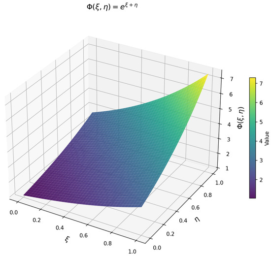
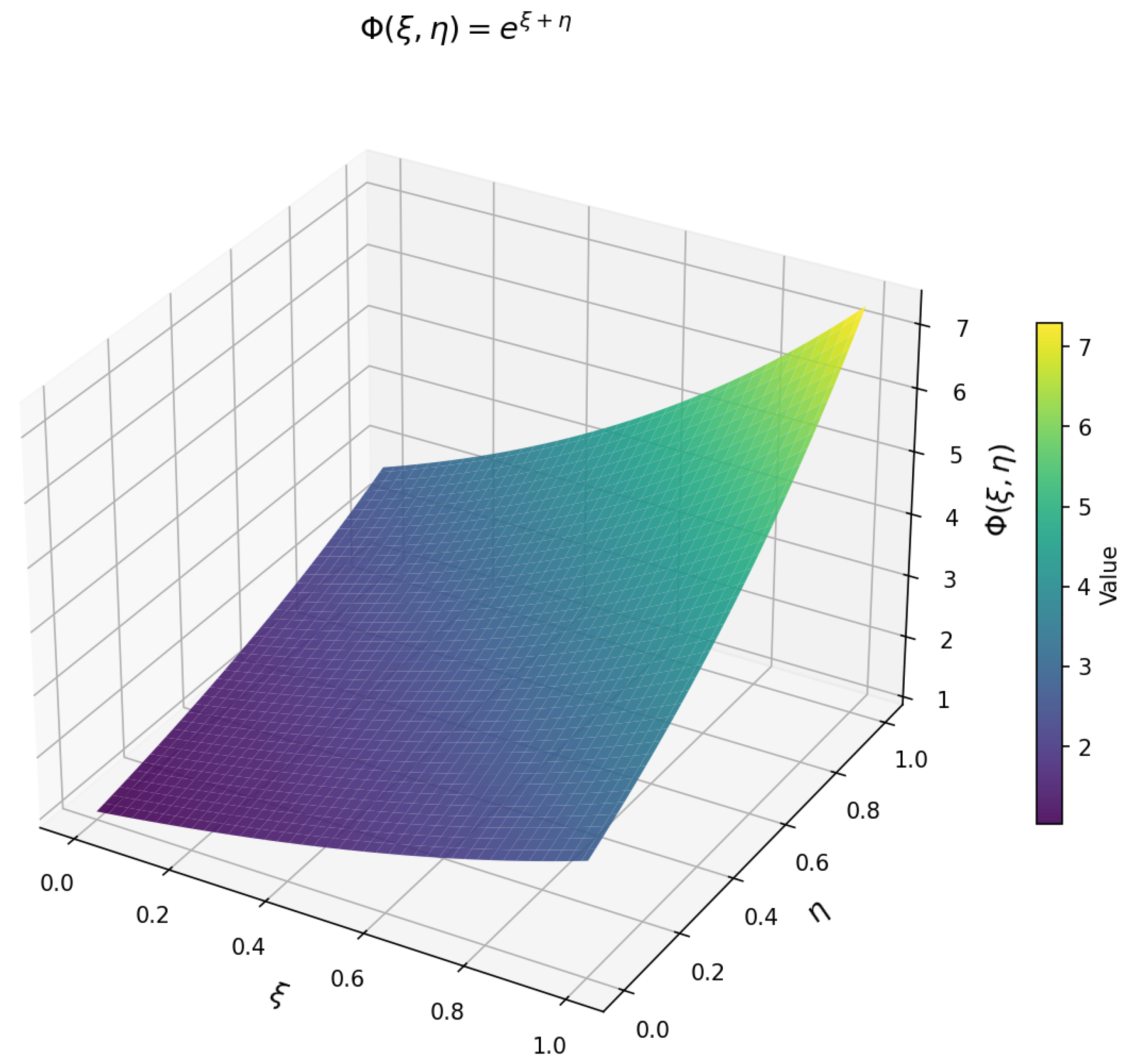
Let Φ ( ξ , η ) = e ξ + η for ( ξ , η ) Ω = [ 0 , 1 ] × [ 0 , 1 ] . Then
2 Φ ξ η ( ξ , η ) = e ξ + η > 0 ,
which is coordinate convex on Ω since e ξ + η is convex in each variable separately. Choosing ς = τ = 1 2 and μ = ν = 1 , so that r 1 = r 2 = 1 2 , we verify Theorem 5.
The left-hand side equals | T 1 + T 2 + T 3 + T 4 | , where
T 1 = 0 1 2 0 1 2 s 1 1 2 s 1 s 2 1 2 s 2 e ( 1 s 1 ) + ( 1 s 2 ) d s 2 d s 1 = e 2 0 1 2 s 1 2 s e s d s 2 0.001970 , T 2 = 0 1 2 1 2 1 s 1 1 2 s 1 s 2 1 2 ( 1 s 2 ) e ( 1 s 1 ) + ( 1 s 2 ) d s 2 d s 1 0.001195 , T 3 = 1 2 1 0 1 2 s 1 1 2 ( 1 s 1 ) s 2 1 2 s 2 e ( 1 s 1 ) + ( 1 s 2 ) d s 2 d s 1 0.001195 , T 4 = 1 2 1 1 2 1 s 1 1 2 ( 1 s 1 ) s 2 1 2 ( 1 s 2 ) e ( 1 s 1 ) + ( 1 s 2 ) d s 2 d s 1 0.000725 .
Thus, the left-hand side is
| T 1 + T 2 + T 3 + T 4 |   0.001970 + 0.001195 + 0.001195 + 0.000725 = 0.005083 .
For the right-hand side, at ς = τ = 1 2 and μ = ν = 1 :
α m = α n = β p = β q = 1 48 ,
so Λ 1 = Λ 2 = Λ 3 = Λ 4 = 1 2304 . The corner values of 2 Φ ξ η are
2 Φ ξ η ( 0 , 0 ) = 1 , 2 Φ ξ η ( 0 , 1 ) = e , 2 Φ ξ η ( 1 , 0 ) = e , 2 Φ ξ η ( 1 , 1 ) = e 2 .
Hence, the right-hand side is
1 2304 1 + e + e + e 2 = ( 1 + e ) 2 2304 0.006001 .
Since 0.005083 0.006001 , the inequality of Theorem 5 is confirmed.
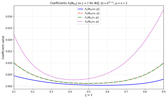
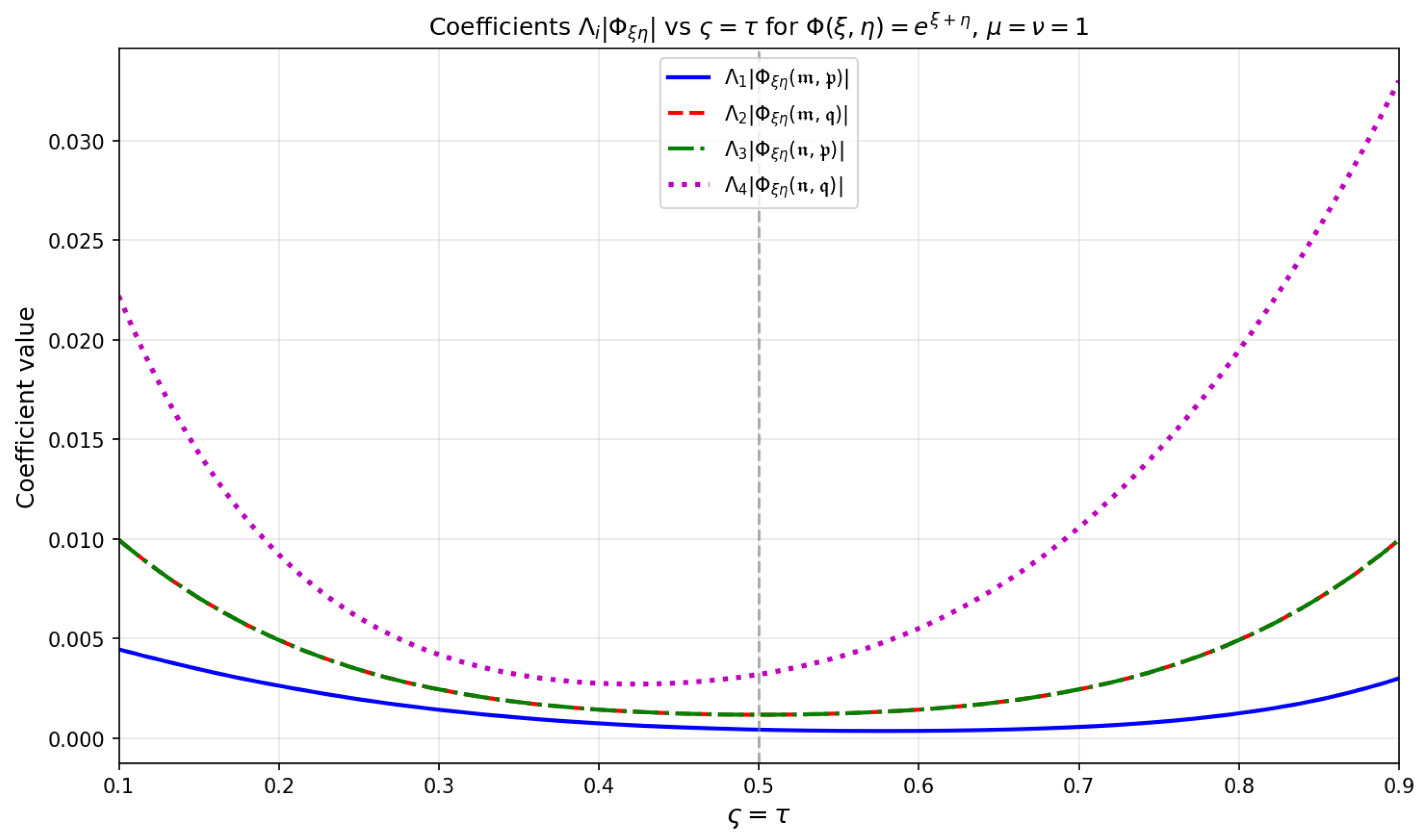
Figure 1 and Figure 2 are presented in this section to help us understand more about the behavior of the inequalities under study. The surface plot of the function Φ ( ξ , η ) = e ξ + η and its mixed partial derivative 2 Φ ξ η = e ξ + η , depicting the coordinate convex structure over the unit square, is given (see Figure 1). Meanwhile, in Figure 2, the left-hand side and right-hand side of the inequality in Theorem 5 are plotted as the parameters ς and τ vary over [ 0 , 1 ] , confirming that the inequality holds throughout and that both sides attain comparable values near ς = τ = 0.5 .

3. Applications to Special Means

In this section, we apply our results to derive some applications involving special means for two variables. For arbitrary positive real numbers m , n , p , q with m < n and p < q , we consider the following:
Arithmetic Mean:
A ( m , n ) = m + n 2 .
Geometric Mean:
G ( m , n ) = m n , m , n > 0 .
Logarithmic Mean:
L ( m , n ) = n m ln n ln m , m , n > 0 , m n .
Proposition 1.
Let m , n , p , q > 0 with m < n and p < q . Setting ς = τ = 1 2 , μ = ν = 1 , and r 1 in Theorem 8, and applying it to the coordinate convex function Φ ( ξ , η ) = ξ 2 η 2 , the following inequality holds:
A ( m , n ) A ( p , q ) 144 1 2304 1 1 r E 1 1 r + E 2 1 r + E 3 1 r + E 4 1 r ,
where
E 1 = 4 r ( m p ) r 192 2 + 4 r ( m q ) r 192 · 64 + 4 r ( n p ) r 192 · 64 + 4 r ( n q ) r 64 2 , E 2 = 4 r ( m p ) r 192 · 64 + 4 r ( m q ) r 192 2 + 4 r ( n p ) r 64 2 + 4 r ( n q ) r 192 · 64 , E 3 = 4 r ( m p ) r 192 · 64 + 4 r ( m q ) r 64 2 + 4 r ( n p ) r 192 2 + 4 r ( n q ) r 192 · 64 , E 4 = 4 r ( m p ) r 64 2 + 4 r ( m q ) r 192 · 64 + 4 r ( n p ) r 192 · 64 + 4 r ( n q ) r 192 2 .
Proof. 
This follows from Theorem 8 applied to Φ ( ξ , η ) = ξ 2 η 2 , for which 2 Φ ξ η = 4 ξ η . Since m , n , p , q > 0 , the function 4 ξ η is convex in ξ for each fixed η > 0 and convex in η for each fixed ξ > 0 , hence 2 Φ ξ η r = ( 4 ξ η ) r is coordinate convex on [ m , n ] × [ p , q ] for all r 1 . The corner values are
2 Φ ξ η ( m , p ) r = 4 r ( m p ) r , 2 Φ ξ η ( m , q ) r = 4 r ( m q ) r , 2 Φ ξ η ( n , p ) r = 4 r ( n p ) r , 2 Φ ξ η ( n , q ) r = 4 r ( n q ) r .
With W i = 1 2304 and M 1 = N 2 = 1 192 , N 1 = M 2 = 1 64 , P 1 = Q 2 = 1 192 , Q 1 = P 2 = 1 64 , the left-hand side | T 1 + T 2 + T 3 + T 4 | = A ( m , n ) A ( p , q ) 144 and the right-hand side is as stated. □
Proposition 2.
Let m , n , p , q > 0 with m < n and p < q . Setting ς = τ = 1 2 and μ = ν = 1 in Theorem 5 and applying it to the coordinate convex function Φ ( ξ , η ) = ξ 2 η 2 , we obtain
A ( m , n ) A ( p , q ) 144 1 2304 2 Φ ξ η ( m , p ) + 2 Φ ξ η ( m , q ) + 2 Φ ξ η ( n , p ) + 2 Φ ξ η ( n , q ) ,
which holds with equality for all admissible values.
Proof. 
This follows from Theorem 5 applied to Φ ( ξ , η ) = ξ 2 η 2 , with 2 Φ ξ η = 4 ξ η . Since m , n , p , q > 0 , the function 4 ξ η is convex in each variable separately, so 2 Φ ξ η is coordinate convex on [ m , n ] × [ p , q ] . With Λ 1 = Λ 2 = Λ 3 = Λ 4 = 1 2304 and corner values 2 Φ ξ η ( m , p ) = 4 m p , 2 Φ ξ η ( m , q ) = 4 m q , 2 Φ ξ η ( n , p ) = 4 n p , 2 Φ ξ η ( n , q ) = 4 n q , the right-hand side becomes
4 2304 m p + m q + n p + n q = 4 ( m + n ) ( p + q ) 2304 = A ( m , n ) A ( p , q ) 144 ,
so the inequality holds with equality, completing the proof. □
Proposition 3.
Let m , n , p , q > 0 with m < n and p < q . Setting ς = τ = 1 2 and μ = ν = 1 in Theorem 5 and applying it to the coordinate convex function Φ ( ξ , η ) = 1 ξ η , the following inequality holds:
A ( m , n ) L ( m , n ) ln A ( m , n ) I ( m , n ) 1 ( n m ) 2 A ( p , q ) L ( p , q ) ln A ( p , q ) I ( p , q ) 1 ( q p ) 2 ( m 2 + n 2 ) ( p 2 + q 2 ) 2304 m 2 n 2 p 2 q 2 ,
where I ( m , n ) = 1 e n n m m 1 n m is the identric mean.
Proof. 
This follows from Theorem 5 applied to the coordinate convex function Φ ( ξ , η ) = 1 ξ η , Φ : ( 0 , ) × ( 0 , ) R , for which 2 Φ ξ η = 1 ξ 2 η 2 . To verify coordinate convexity, note that
2 ξ 2 2 Φ ξ η = 2 ξ 2 1 ξ 2 η 2 = 6 ξ 4 η 2 > 0 , 2 η 2 2 Φ ξ η = 2 η 2 1 ξ 2 η 2 = 6 ξ 2 η 4 > 0 ,
for all ξ , η > 0 , so 2 Φ ξ η = 1 ξ 2 η 2 is convex in each variable separately and hence coordinate convex on [ m , n ] × [ p , q ] . The corner values are
2 Φ ξ η ( m , p ) = 1 m 2 p 2 , 2 Φ ξ η ( m , q ) = 1 m 2 q 2 , 2 Φ ξ η ( n , p ) = 1 n 2 p 2 , 2 Φ ξ η ( n , q ) = 1 n 2 q 2 .
The left-hand side factors as I ( m , n ) · I ( p , q ) , where
I ( m , n ) = 0 1 K ( s 1 ) 1 m s 1 + n ( 1 s 1 ) 2 d s 1 = A ( m , n ) L ( m , n ) ln A ( m , n ) I ( m , n ) 1 ( n m ) 2 ,
with K ( s 1 ) = s 1 1 2 s 1 1 [ 0 , 1 2 ] ( s 1 ) + s 1 1 2 ( 1 s 1 ) 1 [ 1 2 , 1 ] ( s 1 ) . With Λ 1 = Λ 2 = Λ 3 = Λ 4 = 1 2304 , the right-hand side is 1 2304 1 m 2 p 2 + 1 m 2 q 2 + 1 n 2 p 2 + 1 n 2 q 2 = ( m 2 + n 2 ) ( p 2 + q 2 ) 2304 m 2 n 2 p 2 q 2 , completing the proof. □

4. Discussion and Conclusions

This result established a new integral identity for twice partially differentiable mappings and used it to derive several fractional Bullen-type inequalities for functions that are convex on the coordinates via Riemann–Liouville fractional integrals. The results extend the one-dimensional inequalities of Fahad et al. [16] to the two-variable coordinated convex setting.
Upper bounds were obtained through three complementary approaches: Hölder’s inequality, the improved Hölder inequality, and the power mean inequality. Each approach yields bounds of a different character, and together they provide a flexible toolkit for estimating the Bullen-type functional in the fractional coordinated setting. The theoretical results were validated through applications to special means and supported by a numerical example with graphical illustrations, confirming the consistency and sharpness of the derived bounds.
The findings contribute to the growing body of literature on fractional integral inequalities for functions of two variables and provide a unified framework that may serve as a basis for further generalizations.
Several directions remain open for future investigation. One can explore whether the present framework extends to broader classes of convexity on the coordinates, such as h-convex, preinvex, or ( s , m ) -convex functions. Other fractional integral operators, including those of Hadamard, Katugampola, or Atangana–Baleanu could yield meaningful generalizations. Furthermore, investigating whether the derived inequalities admit applications in numerical integration error estimation or in optimization problems involving coordinated convex objective functions represents an interesting open problem.

Author Contributions

Conceptualization, O.B.A. and W.S.; methodology, O.B.A. and W.S.; software, O.B.A. and W.S.; validation, O.B.A. and W.S.; formal analysis, O.B.A. and W.S.; investigation, O.B.A. and W.S.; writing—original draft preparation, O.B.A. and W.S.; writing—review and editing, O.B.A. and W.S.; visualization, O.B.A. and W.S.; supervision, O.B.A. and W.S.; project administration, O.B.A. and W.S. All authors have read and agreed to the published version of the manuscript.

Funding

This research received no external funding.

Data Availability Statement

No new data were created or analyzed in this study, data sharing is not applicable.

Conflicts of Interest

The authors declare no conflicts of interest.

References

  1. Dragomir, S.S. Some Inequalities of Trapezoid Type for Double Integral Mean of Absolutely Continuous Functions. In Mathematical Analysis, Optimization, Approximation and Applications; World Scientific: Singapore, 2025; pp. 227–261. [Google Scholar]
  2. Almutairi, O.B.; Saleh, W. New generalization of geodesic convex function. Axioms 2023, 12, 319. [Google Scholar] [CrossRef]
  3. Hussain, S.; Rafeeq, S.; Chu, Y.M.; Khalid, S.; Saleem, S. On some new generalized fractional Bullen-type inequalities with applications. J. Inequal. Appl. 2022, 2022, 138. [Google Scholar] [CrossRef]
  4. Bullen, P.S. Error estimates for some elementary quadrature rules. In Publikacije Elektrotehničkog Fakulteta. Serija Matematika i Fizika; University of Belgrade: Belgrade, Serbia, 1978; pp. 97–103. [Google Scholar]
  5. Cakmak, M. The differentiable h-convex functions involving the Bullen inequality. Acta Univ. Apulensis 2021, 65, 29–36. [Google Scholar]
  6. Erden, S.; Sarikaya, M.Z. Generalized Bullen type inequalities for local fractional integrals and its applications. Palest. J. Math. 2020, 9, 945–956. [Google Scholar]
  7. Hussain, S.; Mehboob, S. On some generalized fractional integral Bullen type inequalities with applications. J. Fract. Calc. Nonlinear Syst. 2021, 2, 93–112. [Google Scholar] [CrossRef]
  8. Hezenci, F.; Kara, H.; Budak, H. New Results on Bullen-Type Inequalities for Coordinated Convex Functions Obtained by using Conformable Fractional Integrals. Ukr. Math. J. 2025, 76, 1901–1923. [Google Scholar] [CrossRef]
  9. Cakmak, M. Refinements of bullen-type inequalities for s–convex functions via Riemann-Liouville fractional integrals involving Gauss hypergeometric function. J. Interdiscip. Math. 2019, 22, 975–989. [Google Scholar] [CrossRef]
  10. Hezenci, F.; Budak, H. New Inequalities of Bullen-type for Twice-Differentiable Functions via Conformable Fractional Integrals. Int. J. Appl. Comput. Math. 2024, 10, 175. [Google Scholar] [CrossRef]
  11. Zhao, D.; Ali, M.A.; Budak, H.; He, Z.Y. Some Bullen-type inequalities for generalized fractional integrals. Fractals 2023, 31, 2340060. [Google Scholar] [CrossRef]
  12. Sarıkaya, M.Z. On the Hermite–Hadamard-type inequalities for co-ordinated convex function via fractional integrals. Integral Transform. Spec. Funct. 2014, 25, 134–147. [Google Scholar] [CrossRef]
  13. Dragomir, S.S. On the Hadamard’s inequality for convex functions on the co-ordinates in a rectangle from the plane. Taiwan. J. Math. 2001, 5, 775–788. [Google Scholar]
  14. Mitrinovic, D.S.; Pecaric, J.; Fink, A.M. Classical and New Inequalities in Analysis; Springer Science & Business Media: Berlin/Heidelberg, Germany, 2013; Volume 61. [Google Scholar]
  15. Iscan, I. New refinements for integral and sum forms of Holder inequality. J. Inequal. Appl. 2019, 2019, 304. [Google Scholar] [CrossRef]
  16. Fahad, A.; Butt, S.I.; Bayraktar, B.; Anwar, M.; Wang, Y. Some new Bullen-type inequalities obtained via fractional integral operators. Axioms 2023, 12, 691. [Google Scholar] [CrossRef]
Figure 1. Surface plot of Φ ( ξ , η ) = e ξ + η over [ 0 , 1 ] × [ 0 , 1 ] , illustrating the coordinate convex structure of the function used in the example.
Axioms 15 00292 g001
Figure 2. Behavior of the coefficients Λ 1 2 Φ ξ η ( m , p ) , Λ 2 2 Φ ξ η ( m , q ) , Λ 3 2 Φ ξ η ( n , p ) , Λ 4 2 Φ ξ η ( n , q ) of Theorem 5 as functions of ς = τ with μ = ν = 1 and Φ ( ξ , η ) = e ξ + η . All coefficients attain their minimum at the midpoint ς = τ = 0.5 .
Axioms 15 00292 g002
Disclaimer/Publisher’s Note: The statements, opinions and data contained in all publications are solely those of the individual author(s) and contributor(s) and not of MDPI and/or the editor(s). MDPI and/or the editor(s) disclaim responsibility for any injury to people or property resulting from any ideas, methods, instructions or products referred to in the content.