1. Introduction
The relationship between EFs and fluid motion is the focus of the multidisciplinary study of EHD. It merges principles from fluid mechanics, electromagnetism, and charge transport to elucidate how electric forces can influence the behavior of dielectric and electrically conductive fluids. When an EF was applied over a fluid interface, early research revealed the creation of field-coupled interfacial waves [
1]. Nonlinear phenomena, namely interfacial flow instability between two conducting liquids in cylindrical geometry, were the subject of further studies [
2]. In order to pump and control electrolyte solutions, conductivity-driven electrokinetic methods were extensively used in micro- and nanoscale devices [
3]. Under sufficiently powerful EFs, these flows were shown to become unstable, with substantial implications for the design and operation of high-conductivity lab-on-chip systems. The effect of a stable longitudinal EF on nonlinear EHD behavior was investigated, and the results showed that system stability was mostly determined by the ratio of electrical conductivity to permittivity [
4]. The EHD stability of an interface between two viscous fluids enclosed in a channel and exposed to a transverse EF was examined [
5]. Linear interfacial wave instabilities were also examined for scenarios with two finite fluid layers with varying electrical characteristics under a normal EF [
6]. Additionally, a horizontal capacitor configuration was used to investigate the periodic and chaotic responses of electroconductive flow in a weakly conducting, non-isothermal fluid [
7]. In this instance, temperature-dependent electrical conductivity drove the observed dynamics, and three different forms of ambient EFs were used to classify the oscillatory regimes. The EHD stability properties of viscous dielectric liquids have gained great attention due to their importance in a wide range of applied physics and engineering applications, with reported results showing strong agreement with established theoretical predictions [
8]. Furthermore, the EHD instability of a system with an ideal gas covering a viscous liquid was discovered, and the applied EF had a destabilizing effect [
9]. However, depending on the ratio of permittivity to electrical conductivity, it was demonstrated that the EF has two roles in the development of instability in leaky dielectric systems. The present methodology in analyzing nonlinear EHD stability markedly differs from that of prior investigations.
The KHI is a typical interfacial phenomenon that happens when two fluid layers flow past one another with different initial streaming velocities. The ST at the interface typically has a stabilizing impact, resulting in a complex interaction between stabilizing capillary forces and destabilizing shear effects. Even in very simple flow arrangements, this competition results in a broad range of dynamical behaviors. The theoretical basis of KHI at a planar interface dividing two incompressible, immiscible, and non-permeable fluids was established by Chandrasekhar [
10]. However, in reality, many fluids show both viscous and elastic responses, especially over short time scales. Accordingly, subsequent studies concentrated on the instability properties of viscoelastic fluids under the influence of horizontal MFs that were modeled as second-order fluids, such as WB fluids [
11]. These investigations showed that, depending on the type of exponentially variable stratification, the system of stability can be changed between stable and unstable regimes and is extremely sensitive to the underlying physical conditions. In such creations, the extra stress tensor was viewed as an independent variable in the hydrodynamic structure. A mixture of asymptotic and numerical methods was then used to assess the stability of Poiseuille flow [
12]. To clarify viscoelastic instability mechanisms, broader classes of flow configurations were studied, including multidimensional thermodynamic flows, extensional flows, and Taylor–Couette flows [
13]. The EHD stability of two evenly moving WB dielectric liquids was examined in porous media, expanding the reach of KHI [
14]. In the absence of surface charge, the interfacial dynamics were found to be considerably altered by an externally applied EF. Surface wave propagation in Maxwell-type viscoelastic fluids was studied using nonlinear analytical methods [
15]. The nonlinear EHD instability of a cylindrical interface between two WB viscoelastic fluids in a saturated porous medium was investigated further recently [
16]. Using the combined impacts of viscoelasticity, EFs, and porous structures, the current work builds on this vast body of literature to investigate specific elements of KHI under equally complicated physical contexts. The current methodology of studying nonlinear EHD stability significantly diverges from that of previous studies.
Porous media are materials formed of connected spaces or pores that permit fluid movement. The intricate interaction among fluid properties, pore-scale structure, and external driving forces governs fluid movement in these media. By connecting the volumetric flow rate to the pressure gradient and the medium’s permeability, Darcy’s law is employed extensively to explain flow through porous materials. One of the hardest issues in mathematical fluid dynamics is the evolution and stability of an interface between two immiscible fluids. It was demonstrated that both necessary and sufficient stability criteria are satisfied when two immiscible liquids flow across a permeable medium at a moving interface [
17]. However, Darcy’s law is typically only applicable when both fluids behave in a Newtonian manner. The flow of Oldroyd-B fluids through porous media has garnered significant attention because of its importance in a wide range of disciplines, including geophysics, biology, chemistry, and the petroleum industry. In this regard, accurate numerical data for pressure losses as well as vortex size and intensity in planar contraction flows were examined, where computations based on extremely small meshes produced detailed and dependable findings [
18]. Furthermore, the energetic contributions of stresses and velocity components in various flow configurations were investigated to capture both inertial and inertia-less regimes of Oldroyd-B fluid motion [
19]. In the presence of surface charge and interfacial surfactant, the linear stability of an electrified interface dividing two coaxial Oldroyd-B fluids in a permeable medium was studied [
20]. The accompanying dispersion relation was thoroughly examined, and the impact of different governing factors was graphically depicted. The EHD instability at a cylindrical interface was also investigated using both VPT and standard normal-mode analysis [
21]. The RTI was explored under fully saturated conditions involving two superposed horizontal fluid layers within a porous medium [
22].
The renowned Chinese scientist Prof. Ji-Huan He suggested a frequency formulation that was influenced by an old Chinese methodology, by introducing a fresh analytical approach in addressing nonlinear systems. This approach seeks to linearize nonlinear ODEs without resorting to iterative optimization procedures. His approach worked well for a variety of nonlinear situations, but it might not be sufficient for systems with severe nonlinearities, especially those with quadratic terms in periodic patterns [
23,
24,
25]. To solve these inadequacies, El-Dib devised an alternate frequency formulation specifically suited to handle systems with severe nonlinear behavior [
26]. This technique efficiently accommodates large nonlinear interactions and delivers more accurate estimates of oscillation frequencies under such settings. El-Dib’s formulation possesses a notable advantage by directly integrating quadratic nonlinear variables into the governing equations. This trait enhances its adaptability and resilience in difficult scenarios where conventional methods may fail [
27]. Because of its ability to handle complex mathematical structures, the El-Dib technique has proven especially useful in high-energy physics and advanced engineering applications, where complex analytical treatments and highly nonlinear models are frequently needed [
28].
Investigating the interfacial instability between two WB/RE fluids exposed to periodic EFs using a unique paradigm shows considerable experimental relevance and creates opportunities for a variety of cutting-edge technology applications. In order to investigate interfacial deformation, wave propagation, and rupture dynamics in systems consisting of viscoelastic polymer solutions, biological suspensions, and electrically responsive complex fluids, this framework guides the design of laboratory-scale configurations using controlled oscillatory EFs. By enabling a precise assessment of the interplay among fluid elasticity, relaxation times, and EF frequency in triggering or suppressing instability, the proposed approach supports the development of high-fidelity EHD experimental platforms, microfluidic devices with embedded electrodes, and high-resolution diagnostic imaging systems in catching transient interfacial modes. The insights acquired from this approach can greatly improve polymer-processing technologies such as electrospinning, electrospraying, thin-film casting, and fiber manufacturing, where good stability controlling directly affects material morphology and practical performance. Additionally, the framework improves voltage-driven jetting and layering mechanisms in additive manufacturing and EHD printing, resulting in improved feature resolution and less defect generation. Periodic EFs can be used to control droplet breakage, mixing, and the controlled transport of complicated biological fluids in microfluidic droplet creation, lab-on-a-chip manipulation, and encapsulation operations. By enabling customizable and predictable deformation responses under periodic EFs, the discoveries advance smart fluid systems, soft robotics, and dielectric elastomer actuators beyond industrial manufacturing. Overall, this paradigm not only enhances the fundamental knowledge of nonlinear interfacial instability in viscoelastic media but also equips researchers and engineers with robust tools to drive the development of next-generation EHD and polymer-processing technologies. For more clarity, the remainder of this paper is organized as follows.
Section 2 outlines the problem formulation and presents the governing PDEs together with the associated nonlinear BCs. The polar-form approach, for both real and complex coefficients, is introduced in
Section 3. The case of uniform EFs is examined in
Section 4; meanwhile,
Section 5 is devoted to the general case of periodic EFs. The numerical investigations are also presented in
Section 6, and the main findings of the study are summarized in
Section 7.
2. Construction of Issue
An essential formulation for analyzing a new framework commences with coupled EHD viscoelastic governing PDEs. These equations delineate the conservation of momentum, mass, and charge at the boundary of two overlapping fluids. The fluids exhibit distinct elastic and relaxation characteristics and are exposed to periodic EFs. The constitutive relations are expressed using the WB/RE models, utilizing first and second RE tensors to account for fluid memory, elastic recoil, and nonlinear stress effects. The EF is incorporated into the formulation via Maxwell’s equations under the leaky-dielectric assumption, where a periodic electric potential, usually sinusoidal, is given, producing time-varying normal and tangential electric stresses at the interface. The stresses are incorporated into stress balance equations, resulting in a revised dispersion relation that considers electric forcing, viscoelasticity, ST, viscosity contrast, and field frequency. The governing PDEs are expanded using perturbation methods, typically through normal-mode analysis or multiple-scale expansions, to isolate the growth rate of interfacial waves and delineate stability boundaries based on the Deborah number, electric capillary number, relaxation times, conductivity ratios, and oscillation frequency. This cohesive framework offers a robust mathematical basis for forecasting instability onset and elucidates the interaction between periodic EFs and viscoelastic stresses, facilitating precise control strategies in engineering applications in advanced EHD and polymer-processing systems. For additional accessibility,
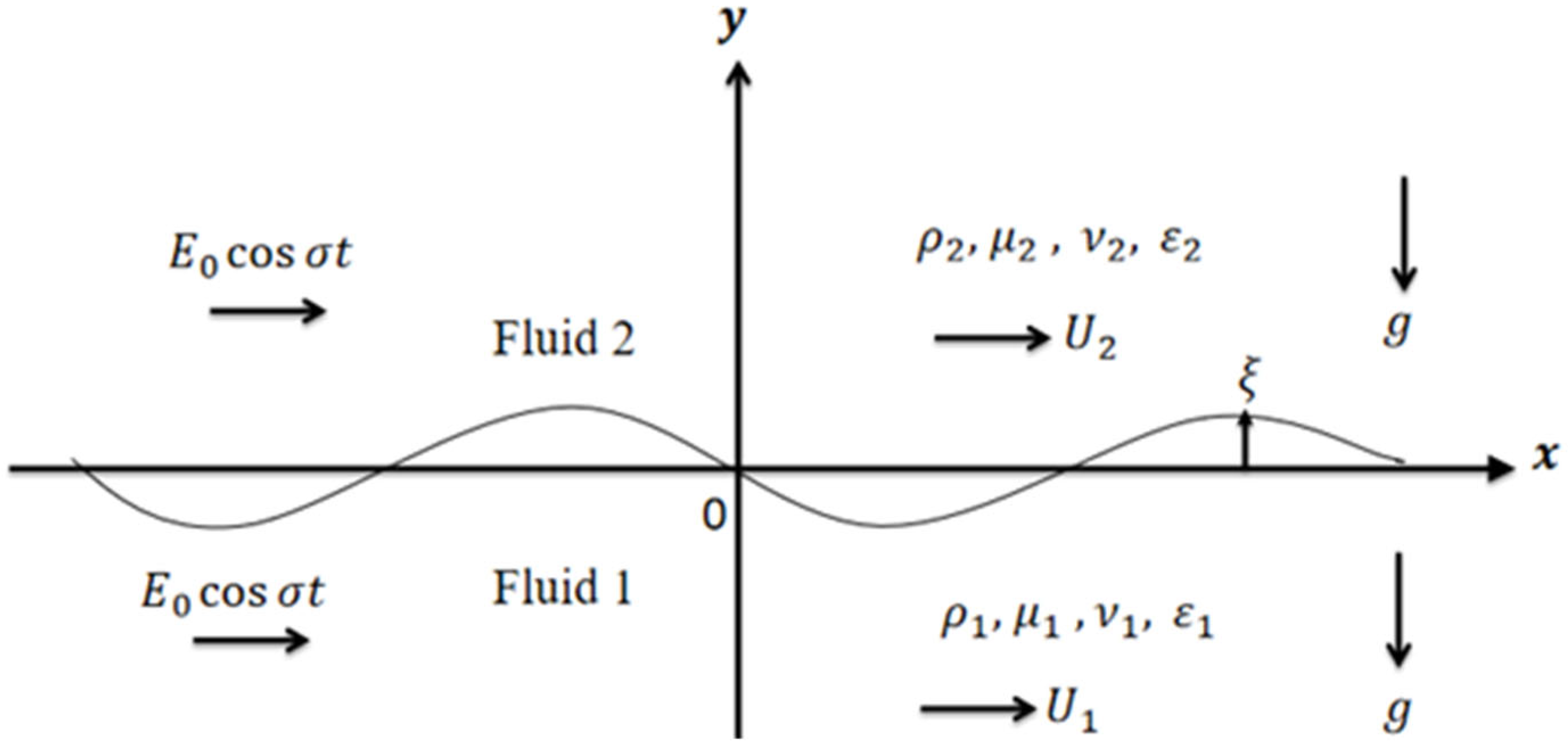
Figure 1 illustrates the physical description of the considered model.
Our system has a typical construction, with the assumption that liquids have different densities, viscosities, and permittivity. Consideration is given to the flow of two WB/RE fluids in semi-infinite layers and filled with a constant and unchanging medium. It is assumed that the two fluids have uniform properties and are incompressible. The plane
is initially formed of an interface between the two fluids, which should be well defined. The
-axis, which corresponds to the undefined flat interface, is reserved horizontally; meanwhile, this axis is taken as vertically upward. Periodic EFs are expected to stress the system.
where the unit vector along the
-axis is denoted by
.
Two uniform initial streaming are existing between the two fluids. The lower and upper fluid characteristics are indicated by subscripts (1) and (2), respectively. Furthermore, the densities and dielectric quantities are referred to as
,
denoted
and
, respectively. There are no electrical volume charge densities because there is no volume charge is assumed. Consequently, only electrical forces affect the interface. The normal component stress in the BCs is affected at the separation surface. Additionally, the gravitational force acts in the negative
-axis as seen in
Figure 1.
and
are kinematic viscosity; meanwhile,
and
are dynamic viscoelasticity, respectively. During permeable media, Darcy’s law governs the movement. The porosity of the two liquids is simply estimated as unity for ease of orientation. A single medium permeability
is given for simplicity’s sake. One way to formulate the surface displacement is as follows [
15]:
where
denotes the horizontal coordinate measured along the interface, meanwhile
represents actual time.
The interfacial deformation describes the deviation of the surface from its initial equilibrium configuration. The increment function can be defined as follows:
Following the standard approach in interfacial stability analysis, the perturbation of the interface is assumed to be harmonic in space, allowing the disturbance to be represented as a sinusoidal wave with time-dependent amplitude.
The interface disturbance’s amplitude is controlled by the arbitrary function
; meanwhile, its spatial frequency is determined by
. Assuming that this function is covered by the Dirichlet BC given below:
When the function
is prescribed with two initial conditions (ICs)
where
is the size of the original disturbance.
The normal mode approach illustrates the rise in a disturbance at the contact as follows:
where the symbol
denotes the complex conjugate of the preceding terms.
The aforementioned form, however, is rather complex and is primarily utilized to facilitate the ensuing mathematical analysis. This formulation provides a convenient framework for examining the interfacial response in a two-phase system, as it compactly describes both spatial and temporal variations in the interface perturbation through complex exponential functions. Such a representation greatly simplifies differentiation and integration when imposing BCs and solving the governing PDEs in the stability examination. Moreover, the sinusoidal structure of the disturbance is well suited of classical stability approaches, including stability analysis, which focuses on tracking the temporal evolution of small-amplitude perturbations. Despite its seemingly elaborate form, this mathematical description is widely employed in fluid dynamics and related disciplines dealing with wave propagation and stability features, as it significantly reduces analytical complexity and computational effort. The central objective of the present study is to determine whether these initial disturbances amplify and drive the system toward instability or decay, thereby restoring the interface to its equilibrium state.
The following is an expression for the interface:
Accordingly, the unit outward normal to the interface is given as follows:
where the unit vector along the
-axis is denoted by
.
The present study has a primary limitation. The primary focus belongs to VPT [
29,
30,
31], which considers viscous or viscoelastic liquids as perfect flows. This notion is employed to derive a precise function of time-dependent displacement of contact. Otherwise, the problem becomes increasingly complex to control. Therefore, we must be thoughtful about this issue. Within this constraint, the flows are supposed to be optimal. VPT provides the benefit of integrating essential viscous factors, including energy dissipation and realistic damping, while maintaining the mathematical simplicity of potential (irrotational) flow. This enables more precise predictions of wave motion, boundary-layer effects, and hydrodynamic forces without the necessity of solving the whole Navier–Stokes equations. Consequently, by applying Bernoulli’s equation, pressure can be removed from the momentum equation. The normal stress BC can be used to express viscoelastic impacts in the current methodology. Accordingly, per our earlier research, the basic equations can be expressed as [
31]:
The positive sign in Equation (9) corresponds to RE viscoelastic prototype, which represents fluids exhibiting a direct (positive) elastic response to deformation; meanwhile, the negative sign refers to WB, which models a delayed (negative) viscoelastic stress response due to relaxation effects.
In Equation (9),
denotes the velocity vector, and
represents the hydrostatic pressure, the parameter
is the gravitational acceleration acting in the negative
-direction, meanwhile
is the unit vector along the vertical axis. The term
represents local acceleration, meanwhile
describes the vector acceleration. The viscoelastic contribution
accounts for elastic relaxation, and the sign convention “(+)” or “(−)” distinguishes between the respective viscoelastic fluid models considered in this study. Because generalizing the KHI of non-Newtonian fluids is a very challenging task, the study is limited to taking weak viscoelastic effects into consideration. The implications of slight viscous effects are standard in the context of Newtonian fluids [
29,
30] and should be treated similarly to a viscoelastic problem since the problem takes relative motions into account. Furthermore, the WB prototype has successfully used the same technology to viscoelastic liquids under the nonlinear stability technique [
16]. The zero-order pure balance of Equation (9)’s structure offers
where the integration constants are denoted by
.
In the equilibrium condition, the normal stress tensor at the separation surface reveals
Based on the principles of VPT, the flow in both liquid layers can be regarded as an irrotational one, in accordance with the fundamental properties of the VPF. Therefore, separate velocity potentials can be introduced for each phase, namely:
The Laplace equation should be satisfied by the potential
because of the following incompressibility condition:
In addition to the two-dimensional limiting perturbations that are included in the momentum PDEs, we will assess the linear PDEs of motion for the two distinct fluid stages. We can conclude that the bulk solutions are distributed normally, as acknowledged by a number of researchers and contingent on an investigation of environmental conditions [
6]. Consequently, by examining normal modes, we can draw the following conclusions:
It should be mentioned that the potential function
arises from the aforementioned structure and the corresponding difficulty. Because of the interface displacement, it is reasonable to assume that
is a limited function that can be obtained. Therefore, in the case of finite solutions, one achieves
where the two finite quantities
and
are involved.
The velocity potentials in both mediums can therefore be represented as follows:
and
where complicated time-dependent constants
and
are needed to be assessed by the applicable BCs.
Using the linear approach, the previously unknown functions are treated as constant values. In contrast, the nonlinear method allows these functions to be expressed in terms of the interface displacement. The pressure can then be determined by applying the procedures derived from Bernoulli’s equation. Specifically, for the WB model, this requires first fully integrating the governing momentum PDE, as indicated in Equation (9).
The dynamic of the existing problem is to depict, simultaneously, using three field equations as follows: the continuity and momentum PDEs together with Maxwell’s equations. The latter equations are derived in light of the quasi-approximation concept [
1]. Focusing on instances of electric energy storage is the aim of the electrified fluids. In contrast, the dispersion times of electromagnetic waves and magnetic energy storage are so small that they can be disregarded. Therefore, the EF can be obtained using a scalar function as [
16]. Consequently, the perturbed EF can be represented as follows:
The elector-quasi-static approximation will include condensing Maxwell’s equations as:
Considering that the dielectric constants are homogeneous, one derives by inserting Equations (13) and (14) to attain
Accordingly, the electric potentials in both media may be represented as follows:
and
where
and
must be computed from the BCs and are affected by temporal quantities.
To this end, the general solutions for both the electric and hydrodynamic components have been fully established. To solve the given problem, the relevant BCs should be supplied in the next subsection.
Nonlinear BCs
The BCs are essential in EHD stability as they govern the interaction of EFs, fluid dynamics, and ST at the system’s boundaries, thereby affecting the propagation or attenuation of disturbances. In situations with charged interfaces or dielectric–conductive fluid layers, specifying conditions like electric potential, charge continuity, velocity constraints, and stress equilibrium at solid boundaries or fluid–fluid interfaces directly affects the interplay between electrical and hydrodynamic forces. The BCs influence the distribution of electric stresses, potentially amplifying perturbations, altering flow patterns, or inducing interfacial instabilities such as electro convection or Taylor–Melcher instabilities. Precise BCs are essential in predicting stability thresholds, characterizing mode structures, and ensuring physically consistent solutions in EHD stability analyses. Two types of BCs can suitably restrict the field equations. Therefore, the interface BCs fall into three categories: electric BCs, stress balancing, and the kinematic BCs of the existing model. The equation representing the physical behavior at the fluid interface must satisfy both the horizontal and vertical components of the fluid velocity. The solutions of Equations (16), (18), (20), (22) and (23), which reflect the velocity and electric potential distributions, should satisfy the following nonlinear BCs [
2,
4,
6,
8,
9].
The following is found at the free interface :
- ➢
At the surface of separation , where this materialist derivative operator is displayed, known as kinematic condition, also referred to as the conservation of mass across the interface. Note that the different fluid zones will be utilized repeatedly. Therefore, this material criterion offers the following in light of Equations (16) and (17).
Consequently, the velocity potentials’ special solutions are as follows:
and
- ➢
The following BCs are required for the electric potential at the separating surface:
- ➢
The component of tangential EF remains unchanged across the interface. Hence, one finds
Equations (19), (22) and (23) are used to attain Equation (27).
- ➢
At the boundary surface, the normal component of electric displacement is continuous, one gets
Equations (19), (22), (23) and (29) are provided
Consequently, the responses to Equations (28) and (29) give
and
Equations (10), (25) and (26) can be substituted into Equation (18), yielding the hydrodynamic pressure. So, one receives
and
Two forces must be considered by the stress tensors. The first force is the electrical stress tensor, which has the following formula:
where the Kronecker delta is indicated
.
The second condition relates to the surface force, which is generated by the Newtonian effect as well as the elastic contributions of the existing model.
In accordance, the operating total stress tensor can be expressed as follows:
The remaining BC is linked to the discontinuity of the normal stress tensor by ST quantity to examine the nonlinear instability analysis. One way to communicate this restriction would be [
21]:
Here
stands for the total force acting on the interface, which is precisely described as follows:
where the components of the unit normal vector directed outward
are denoted by
and
.
One way to express the unit normal vector’s divergence up to the third order is as follows:
. The nonlinear distinguishing equation is the situation’s essential component. This equation may be formulated by replacing Equation (38) with Equations (25), (26), (31)–(34) and (37), respectively. Long and easy calculations are required. In reality, a nonlinear PDE is the characteristic equation. We will perform the derivatives of the coordinate x in order to transform the PDE into an ODE one because our goal is temporal instability. After that, we will simply substitute
. To put it simply, imagine that an observer is at the origin, watching the interface displacement wave’s behavior as a function of time. In the end, the surface displacement’s non-dimensional ODE might be written as follows:
where
where the temporal differential is indicated by the prime.
The following dimensionless numbers are produced using a non-dimensional process:
The Weber numeral , the viscoelasticity parameter , Darcy number the Ohnesorge number and . The star will be eliminated to make things straightforward. Several rigorous procedures can be used to simplify the equation, while maintaining its fundamental dynamics to make dealing with the extremely complex Equation (40) easier, especially without the need for traditional perturbation techniques:
4. Special Case: Uniform Electric Field ()
Analyzing the typical situation in which the periodic EF transitions to a non-periodic state is beneficial for a deeper comprehension of the EHD reaction of the system. A time-independent DC of EF is produced when the EF frequency is adjusted to zero
. A direct comparison between steady electric forcing and the totally periodic excitation studied in the general model is made possible by the situation
, which eliminates the temporal modulation of the forcing term. From a mathematical standpoint, all terms and coefficients that explicitly depend on
in the nonlinear characteristic equation driving the interface motion are eliminated when
is imposed. Consequently, an autonomous ODE with constant coefficients replaces the general equation with time-dependent coefficients. The reduction can be expressed in a representative form as
To preserve the basic dynamics of the original nonlinear system, a new formulation is proposed that explicitly captures the quadratic nonlinearity. This approach offers a more effective means of understanding the system’s behavior while maintaining the intrinsic characteristics of the nonlinear oscillator. This makes it possible to determine the system frequency and provide a relevant solution to the issue. Accordingly, it is possible to rewrite Equation (45) in such a way that the restoring force is impacted by the quadratic nonlinearity:
where
and
where
collects damping contributions (viscous, porous, and viscoelastic effects), and
collects the restoring nonlinearities (quadratic/cubic) transported by ST and the geometry-dependent Maxwell stress. The natural frequency
and the damping nonlinear coefficients become time-independent in the reduced form because there is no periodic forcing. Physically, the oscillating EF’s parametric energy injection is turned off when
. Consequently, the near-resonant parametric excitation instability bands vanish, and the primary stabilizing processes that regulate the interface dynamics are viscoelastic elasticity (as measured by the viscoelasticity number), porous resistance
, viscous dissipation, and ST. In the absence of time-dependent excitation, the response exhibits greater damping, and the stability zone in wave number space typically increases compared to the
situation. Accordingly, this unique case can be used as a baseline configuration to accurately quantify the specific impact of periodic electric excitation on stability bounds and growth rates. The linearization of Equation (45) around the quiescent state yields the standard second-order form.
where
where
and
Finally, the entire equivalent frequency can be written as
. where
collects viscous, porous, and viscoelastic dissipation, and
represents the effective (dimensionless) damping ratio at
. Asymptotically, the interface is stable if
We focus on the functional relationship represented by Equation (51). Plotting the logarithm of the EF strength against the wave number of the surface waves allows for the investigation of this relationship, as seen in the accompanying images. The NS and corresponding analytical solution of the analogous equation given in Equation (49) are found using the following procedure:
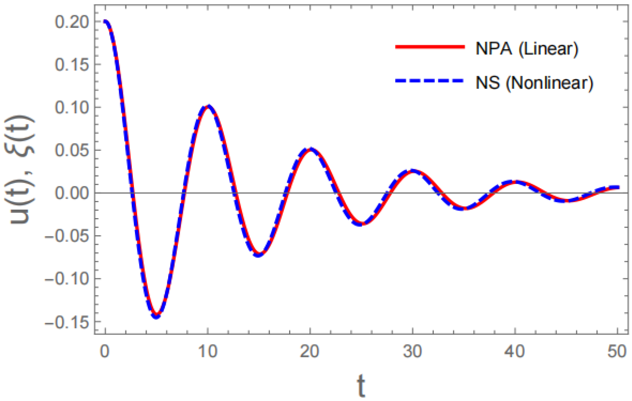
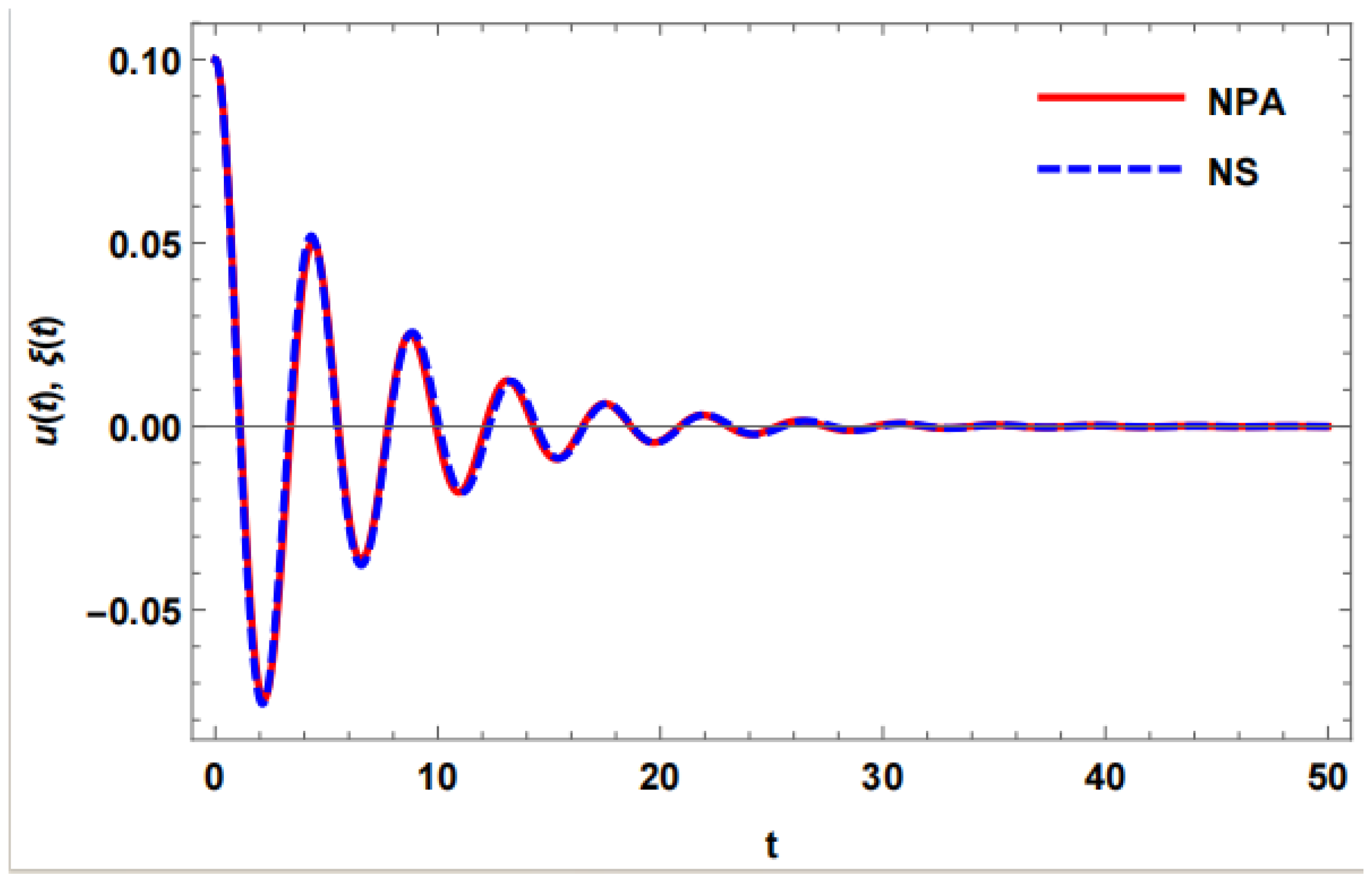
To validate the NPA, the NS of Equations (45) and (49) are shown in
Figure 2. The solid red curve relates to Equation (49); meanwhile, the blue curve shows the result for Equation (45). The results are almost the same, differing with an absolute error of 0.00487345, as shown by the tight alignment of these two curves. This small difference shows that both equations produce very consistent responses, highlighting the great degree of accuracy and dependability attained by the numerical processes. Such broad consensus implies that the methods developed to solve these ODEs are sound, with real-world uses in confirming the accuracy of theoretical predictions in liquid dynamics or related domains and validating computational models. The numerical values of the other parameters are selected as follows:
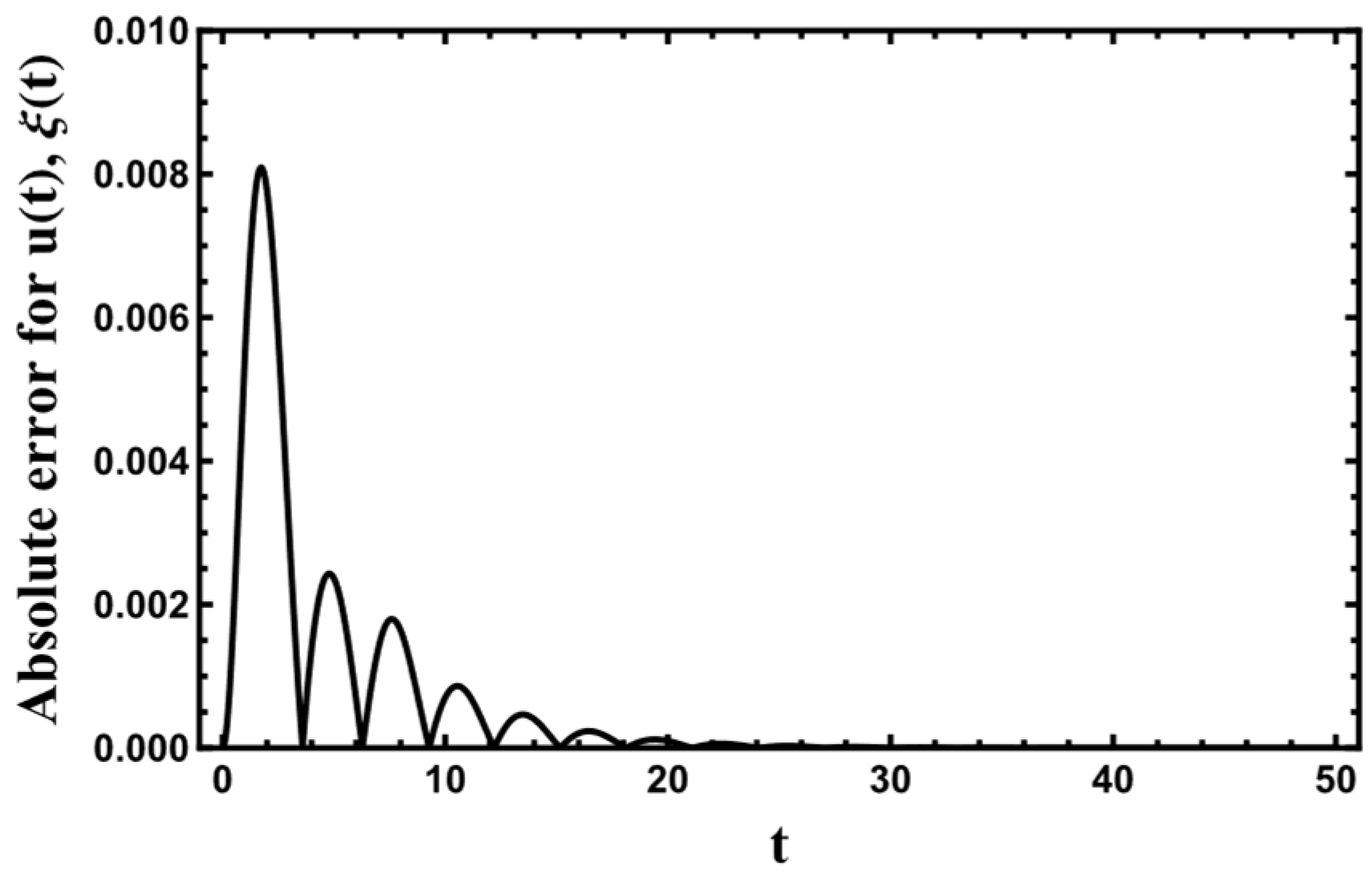
For more clarity, an absolute error curve is depicted as follows:
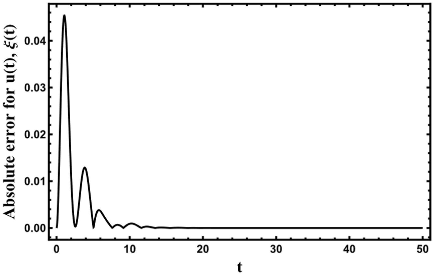
Figure 3 illustrates the temporal progression of the absolute error associated with the state variables
and
, offering a clear understanding of the transient and asymptotic characteristics of the proposed system. The error trajectory displays a significant early peak, succeeded by a swiftly diminishing oscillatory response, typical of a stable underdamped dynamical system. During the initial phase
, the absolute error escalates rapidly to a peak value on the order of
. This temporary enhancement illustrates the system’s susceptibility to initial conditions and the prompt initiation of the dynamic reaction. Nevertheless, this peak is ephemeral, and the system swiftly shifts into a damping phase. Consequently, the error exhibits oscillations with progressively diminishing amplitude, signifying the existence of efficient dissipative mechanisms. The envelope of the error decay indicates a roughly exponential convergence rate, serving as a robust indicator of asymptotic stability. The oscillations are precisely regulated and demonstrate no increase or irregularity, hence verifying the lack of instability or numerical artifacts. As time advances
, the error converges to zero with a few residual oscillations, indicating superior tracking performance and strong steady-state behavior. The uniformity and consistency of the decay profile indicate that the system is both stable and well-conditioned under the specified parameter values.
Figure 3 presents persuasive evidence that the suggested model accomplishes swift transient suppression, effective error dissipation, and assured long-term convergence. These attributes highlight the system’s resilience and reliability, rendering it suitable for real applications where stability and accuracy are essential.
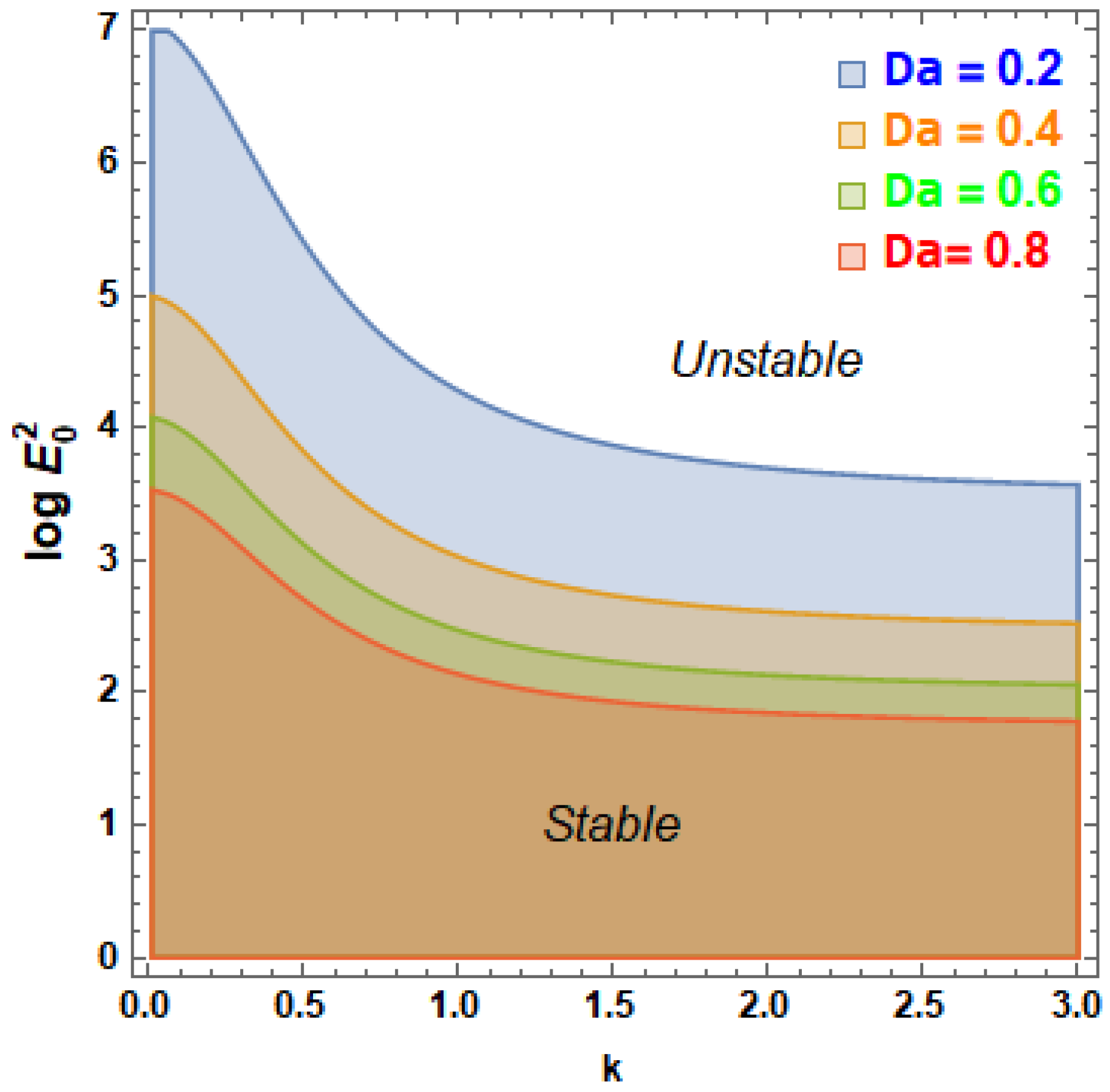
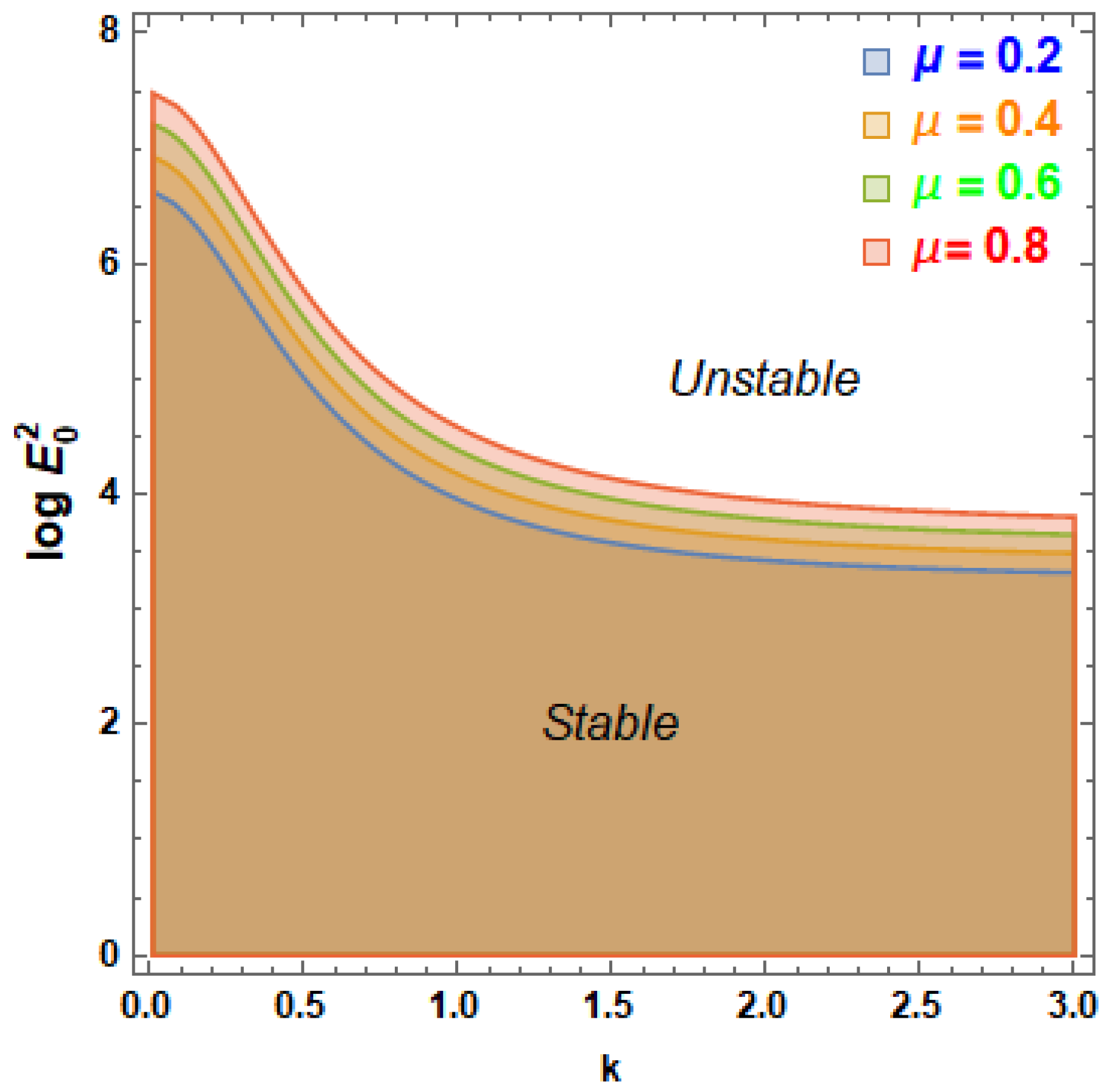
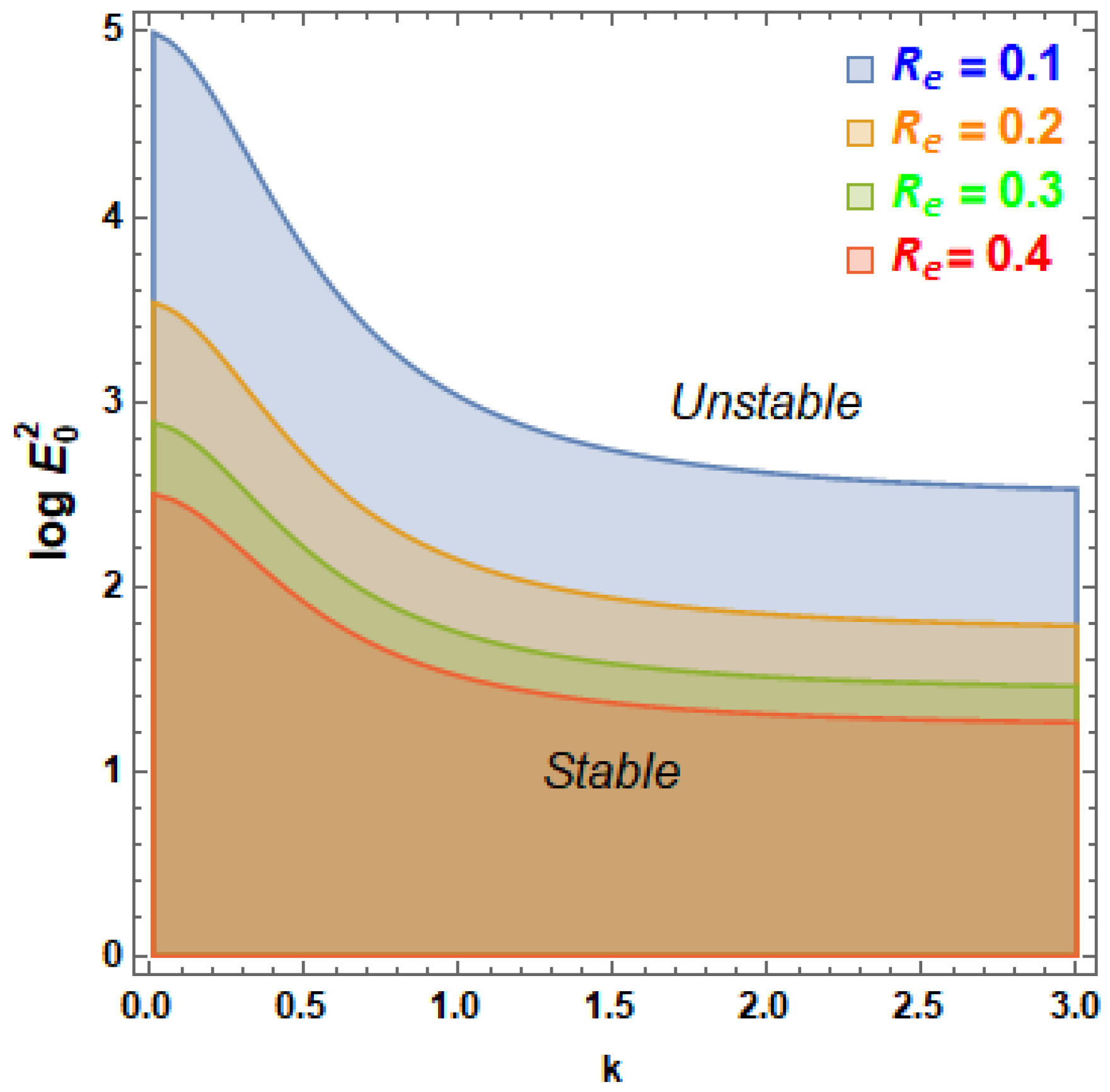
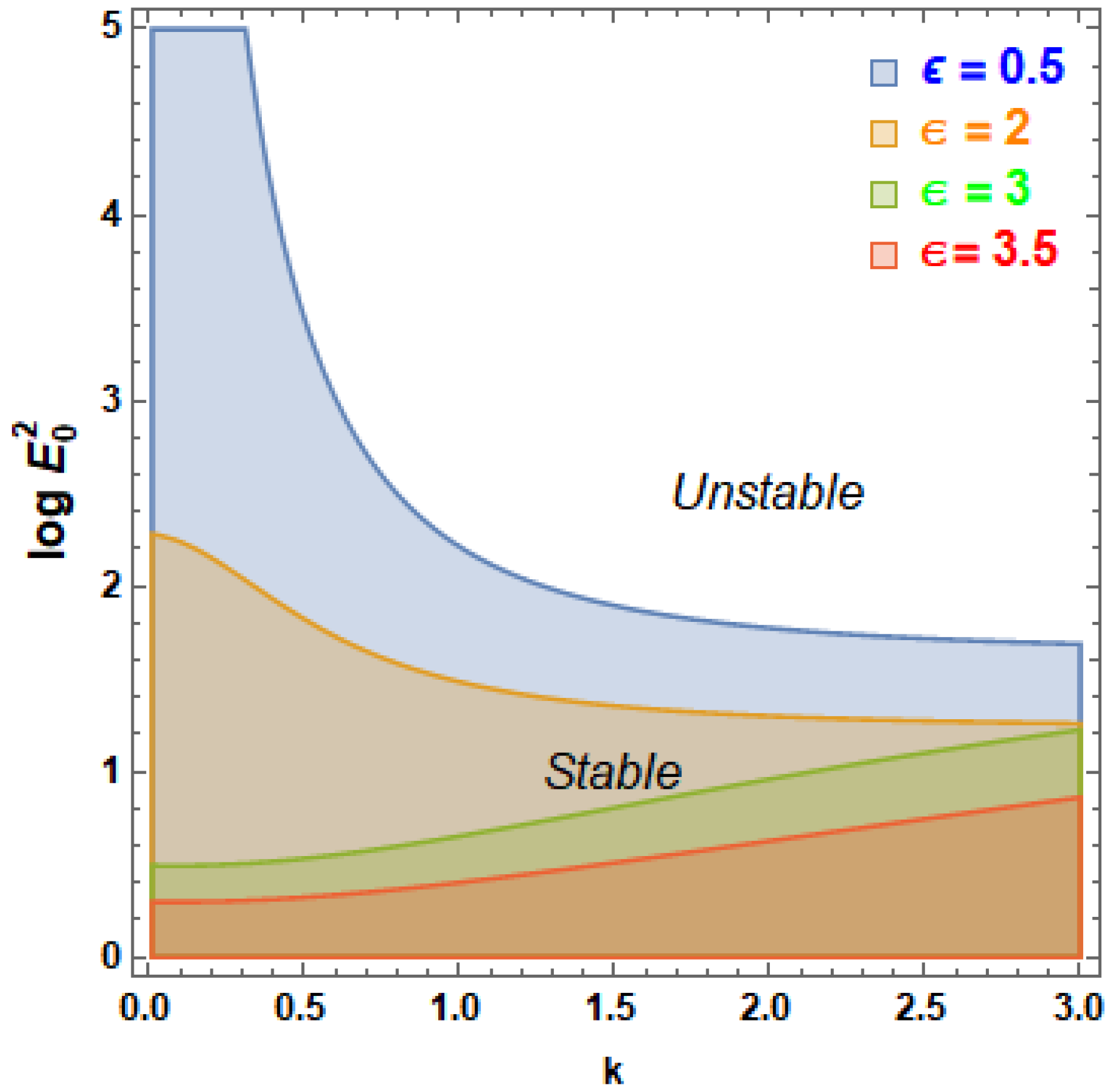
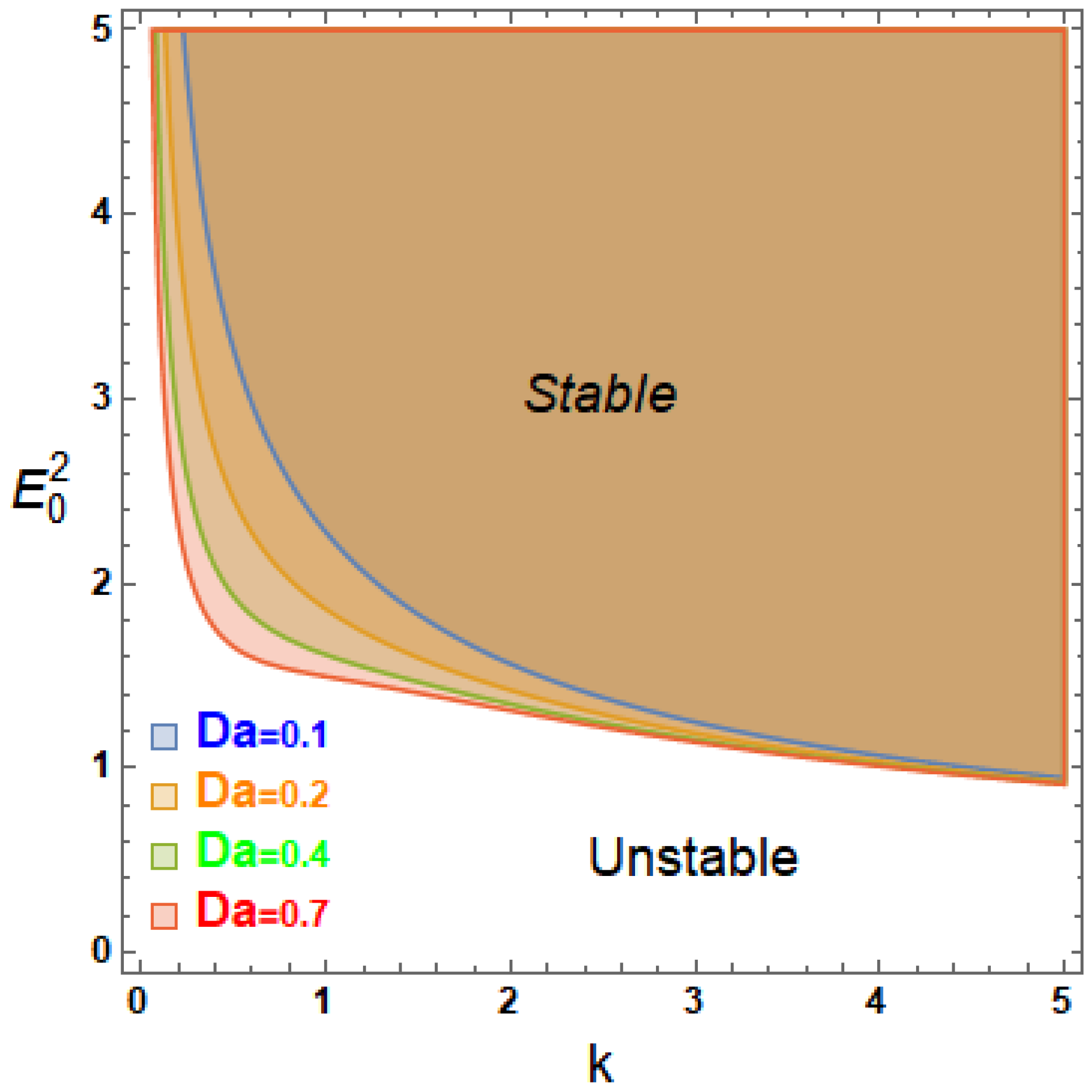
Figure 4,
Figure 5,
Figure 6 and
Figure 7 show the stability bounds of
vs.
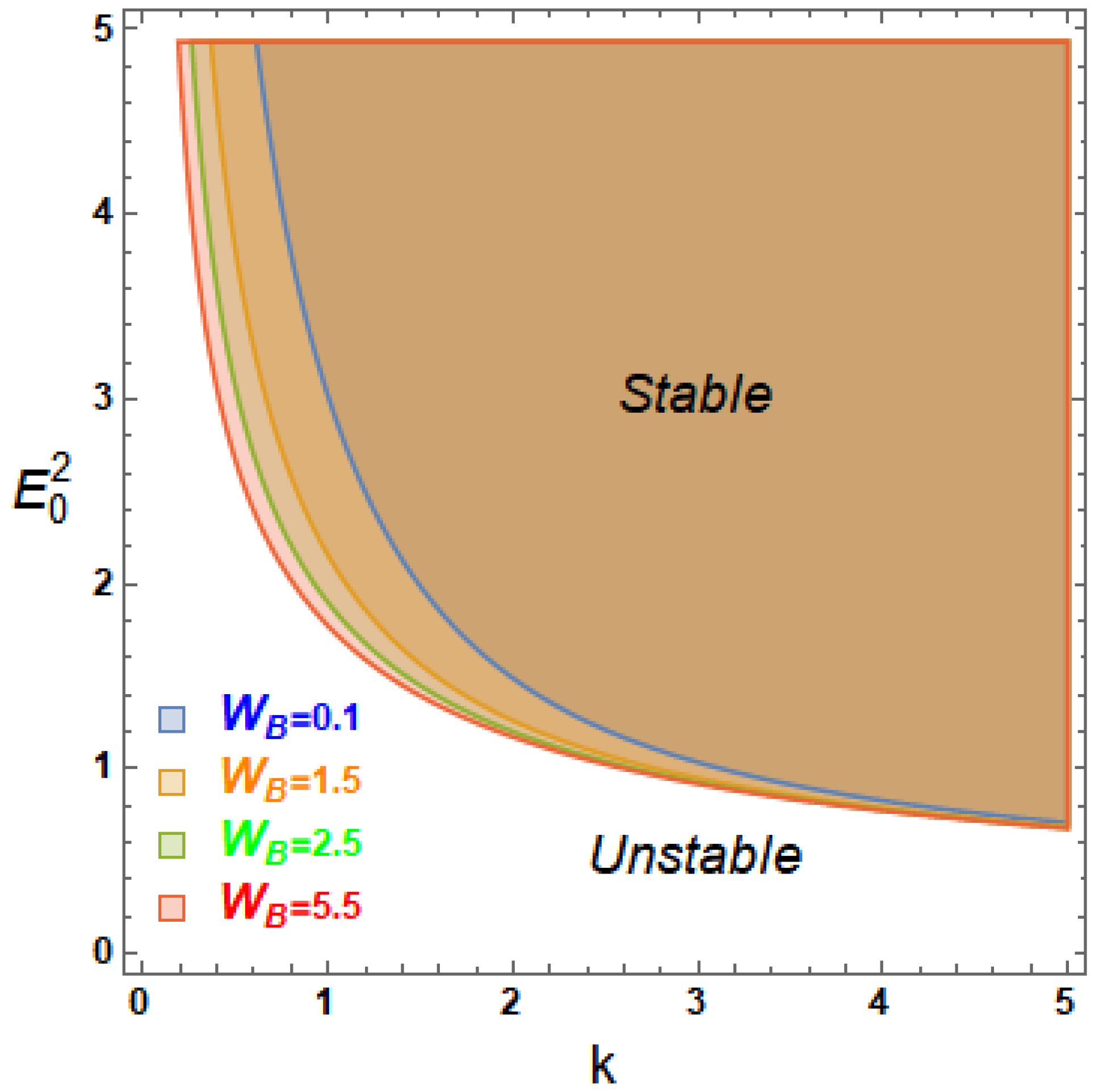
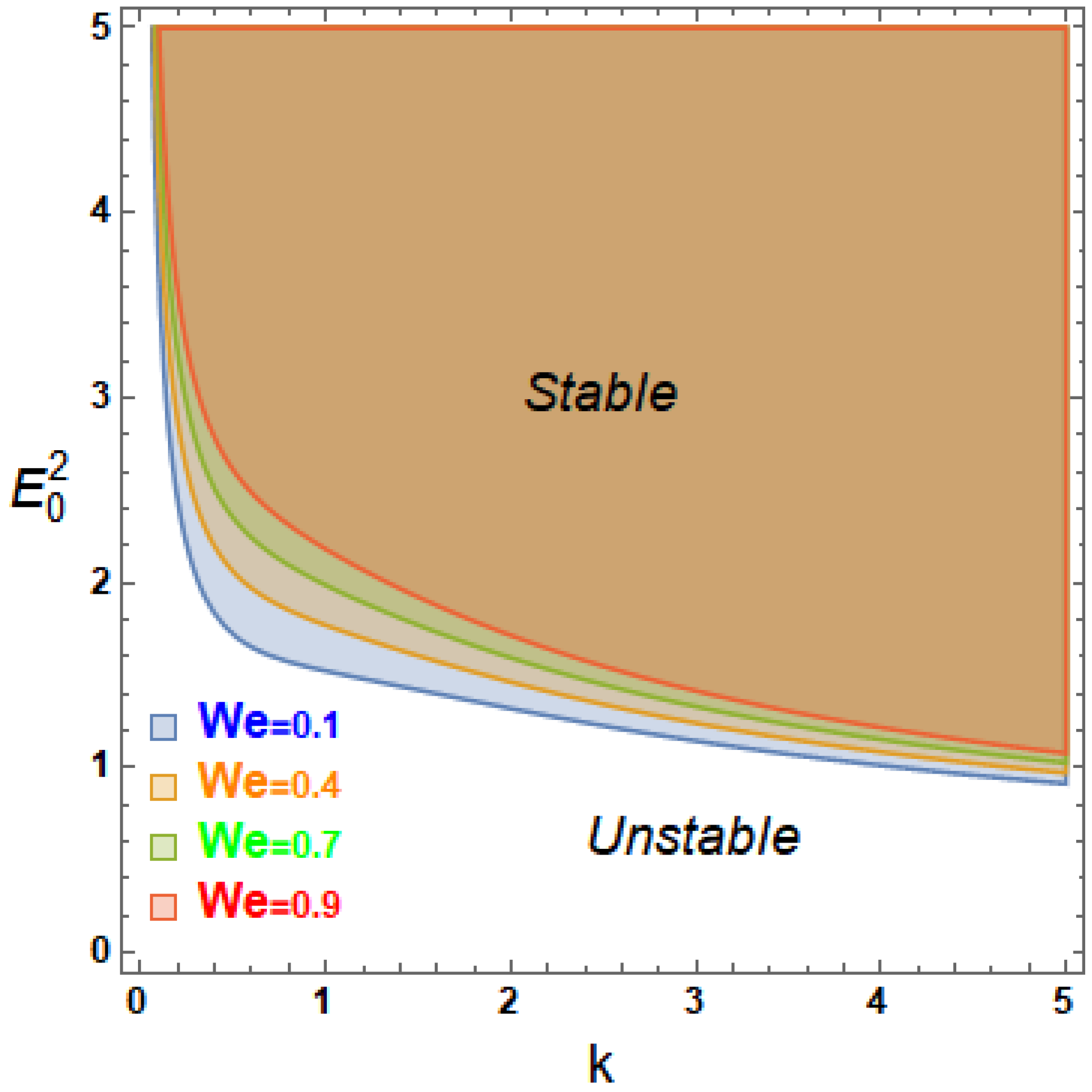
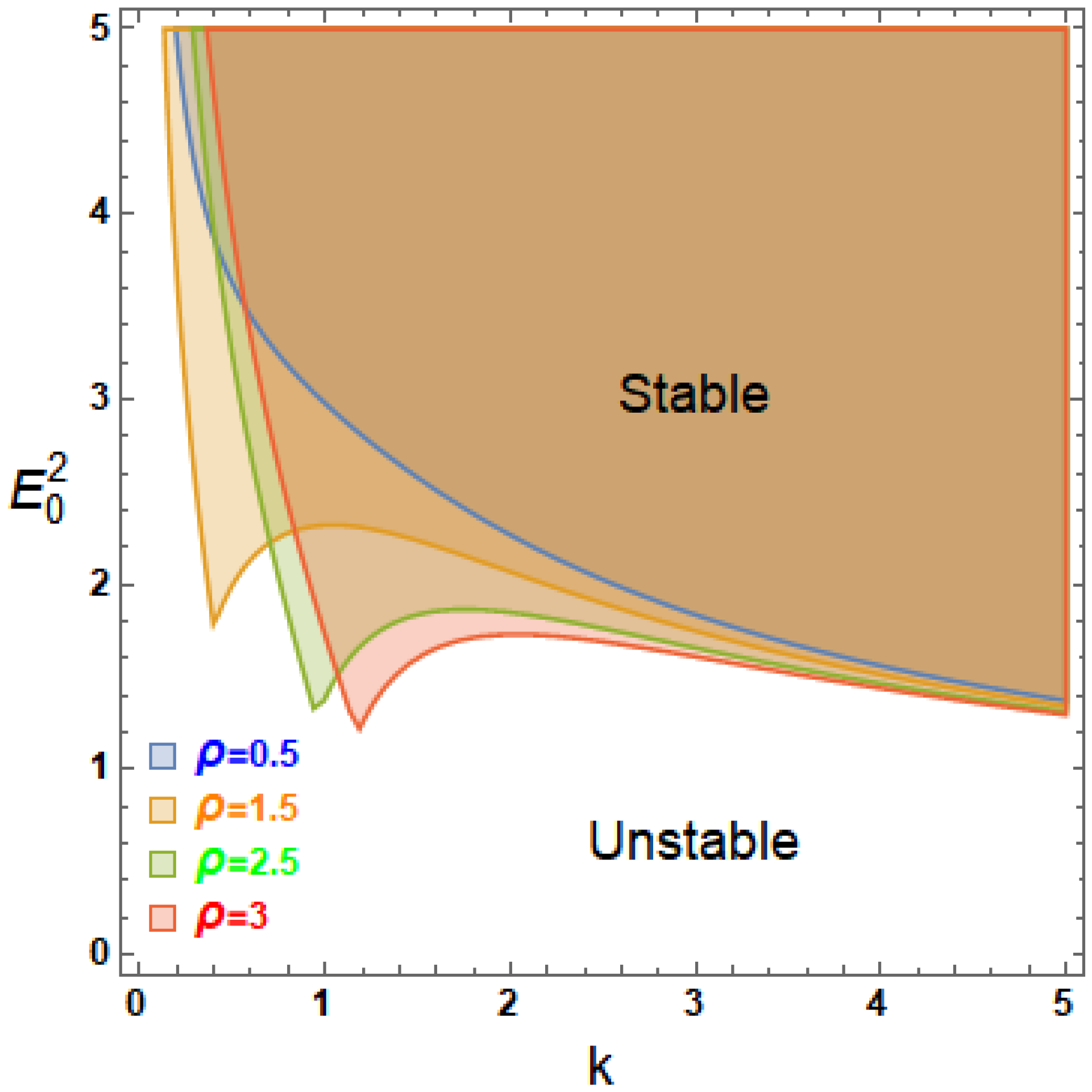
plane. To clearly illustrate each parameter’s independent influence, the curves are drawn for representative values of the key regulating parameters, with just one parameter being changed at a time in each figure, while the others are kept constant. Equation (53) can be rewritten as an inequality
under the restriction
where the coefficients
are functions of all the system’s physical characteristics. Additionally, the numerical analysis shows that for any
, demonstrating the destabilizing effect of the EF, which is consistent with earlier findings [
16,
32,
33]. As shown in
Figure 4,
Figure 5,
Figure 6 and
Figure 7, the stability characteristics are represented using the solution in terms of
vs.
for easier presentation and useful interpretation. The stability zone is represented by the shaded part of the graph, which is indicated by the term “stability,” while the unstable area is represented by the unshaded area, which is indicated by the term “instability.”
In
Figure 4, the Darcy number
is used in the figure to show how medium permeability affects stability characteristics. It is evident that the zones of instability increase as
increases; meanwhile, all other parameters remain unchanged. Consequently, the system is unstable in this instance. This was similar to what was previously validated in [
9].
Figure 5 illustrates the stability distribution’s
ratio inspection. The non-dimensional EF intensity
is shown against
in this figure. The values of the other parameters remain constants; the viscosity factor ratio varies between 0.2 and 0.8. It is observed that the stabilizing areas are improved as the amounts of
increased, particularly for greater amounts of
. Consequently, it is concluded that
has a stabilizing effect. It has been shown that the dynamic viscosity ratio has two roles in the allocation of instability, notwithstanding various restrictions [
33].
In
Figure 6, stability curves show that the Reynolds number
consistently affects when instability first appears. The critical values of
drop over the whole wave number
range as
rises from 0.1 to 0.4, suggesting that instability is induced at lower EF intensities as inertial effects intensify. This pattern demonstrates that inertia has a destabilizing role in the EHD system under consideration. By reducing interfacial disturbances, viscous dissipation dominates stabilization at relatively low
, creating a larger stable area. This viscous repression is weakened, and disturbances can arise more readily as
increases. Stronger inertial effects expand the unstable domain at the expense of the stable one from a physical standpoint by improving momentum transport and encouraging the amplification of electrically induced interfacial perturbations. These findings demonstrate that
are a useful control parameter in adjusting the system’s interfacial stability properties.
The effects of the dielectric factor
on the stability zone are seen in
Figure 7. With the exception of the dielectric factor
, which takes the values as, all the physical factors are held constant
. As seen from this image,
has a destabilizing function in the stability distribution, especially when
is higher. Furthermore, it is discovered that as
increases, the number of instability areas and the escalating rate of apportionment rise sharply. Furthermore, it can be shown that the non-dimensional inclined EF is significantly impacted by the increase in this parameter. Accordingly, the liquid’s outer dielectric factor has grown. Consequently, it can be concluded that
destabilizes the system in question [
33].
5. The Periodic Electric Field General Case
There are cubic and quadratic terms in the nonlinear Mathieu Equation (44). Due to parametric excitation-induced natural frequency disruptions, the system enters a non-autonomous state. The system can, nevertheless, develop into an autonomous state by approximating these changed natural frequencies with an estimated constant frequency. This method was earlier discussed [
34,
35,
36]. Consequently, the following is a rewriting of Equation (44) as an autonomous structure [
37]:
This independent equation eliminates the complexity related to changeable coefficients, making it easier to analyze the dynamics of the system. The constant coefficients of the variables
are listed below, and this reformulation makes it easier to examine stability and resonance behavior in the system:
and
In order to preserve the fundamental dynamics of the original nonlinear system, a new representation purposefully reconfigures the quadratic nonlinearity [
38]. The method provides a more useful means of comprehending the behavior of the system. El-Dib [
27] first included a quadratic stiffness component to the constitutive equation to generate the system frequency and develop the solution to the problem while considering the influence of the quadratic nonlinearity. This was accomplished by using a cubic term for integration across the variable
as opposed to a quadratic term. Consequently, Equation (53) can be rewritten so that the quadratic nonlinearity affects the restoring force as
where
and
The nonlinear ODE as given in Equation (57) governs the temporal evolution of the interfacial disturbance and exhibits several important dynamical features. The term acts as an effective damping mechanism whose magnitude depends on the instantaneous displacement, reflecting the combined influence of porous resistance and viscoelastic effects. Meanwhile, the restoring force represented by incorporates both elastic and EHD contributions, producing a displacement-dependent stiffness that modifies the natural oscillatory character of the system. The periodic electric forcing is embedded in the coefficients, introducing additional modulation, resulting in oscillatory or weakly damped responses depending on parameter values.
As a consequence, the interface behaves as a damped and periodically forced nonlinear oscillator whose amplitude, dominant frequency, and stability depend sensitively on the interplay among Darcy resistance, viscoelastic elasticity, inertial effects, and EF excitation. For small perturbations, the solution tends to remain bounded; meanwhile, stronger inertial effects or reduced porous resistance lead to amplified oscillations and possible loss of stability. This interpretation clarifies the physical implications of Equation (57) and provides a bridge between the nonlinear model and the subsequent linearized analysis.
This change facilitates the analysis of the nonlinear Equation (57), where the quadratic nonlinearities contribute to the restoring force but are strategically balanced or converted into an equivalent cubic effect. This reconfiguration provides a more analytically tractable and dynamically correct description of the system, enabling a better comprehension of resonance, stability, and oscillatory behavior.
The linear equivalent of Equation (49), which can be expressed as
A trial solution to Equation (57) can be displayed as follows to obtain the natural frequency
and damping coefficient
:
Later on, the initial amplitude A and total frequency Ω of the oscillation will be determined. It should be noted that the trial solution satisfied the initial specifications given in Equation (4).
The linearized form is obtained by estimating the natural frequency
and damping coefficient
as follows:
and
The solution to Equation (60) takes the following form:
where it is established that the total frequency corresponding to the aforesaid solution is given as:
The frequency equation is a quadratic in the following, when Equations (62) and (63) are added to Equation (65).
Certain requirements must be met for stability, depending on the system being studied. Generally speaking, the stability of a system is determined by the following basic concepts:
6. Numerical Discussions
This Section discusses the influence of the physical properties underlying the mathematical system under study on the ultimate analytical solution as given in Equation (64). The numerical computations of the solution
under the impact of
are displayed in
Figure 8,
Figure 9,
Figure 10,
Figure 11,
Figure 12,
Figure 13 and
Figure 14 for a sample chosen system as follows:
In
Figure 8, the numerical solution of the appropriate linearized ODE, as shown in Equation (60) (blue curve), and the nonlinear ODE given in Equation (45) (red curve) are contrasted. Strong consistency between the nonlinear and linear formulations is indicated by the two curves’ extremely close agreement. The proposed numerical scheme’s great accuracy and dependability are confirmed by the minor difference between them, which can be measured by an absolute error of roughly 0.000449031. This slight variation implies that the numerical process reproduces the dominating dynamics anticipated by both models and accurately depicts the fundamental physical behavior of the system. The two solutions’ near overlap increases confidence in the reported results and demonstrates how well the computational approach handles such difficult ODEs.
To enhance clarity, an absolute error curve is illustrated as follows:
Figure 9.
Demonstrates the temporal evolution of the absolute errors for .
Figure 9.
Demonstrates the temporal evolution of the absolute errors for .
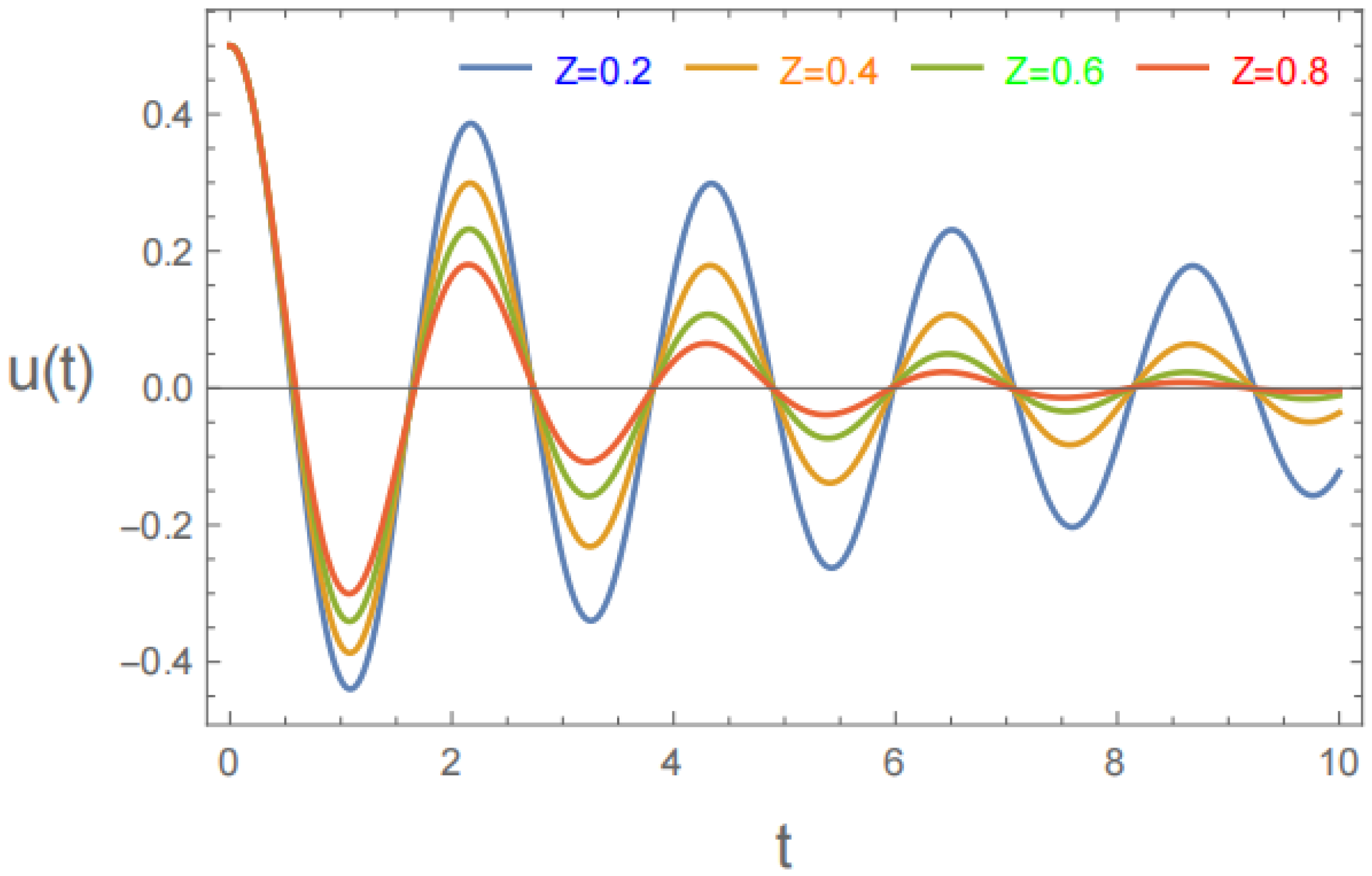
Figure 10.
Shows the effect of changing on the solution (56) for the system.
Figure 10.
Shows the effect of changing on the solution (56) for the system.
Figure 11.
Displays the variation of
for the same system is given in
Figure 2.
Figure 11.
Displays the variation of
for the same system is given in
Figure 2.
Figure 12.
Shows the variation of for the same system.
Figure 12.
Shows the variation of for the same system.
Figure 13.
Shows the variation of for the same system.
Figure 13.
Shows the variation of for the same system.
Figure 14.
Shows the variation of for the same system.
Figure 14.
Shows the variation of for the same system.
Figure 9 depicts the time progression of the absolute error related to the state variables under an alternative
system setup. The error dynamics display a significant transient peak, succeeded by a swiftly diminishing oscillatory pattern, hence reinforcing the stability attributes of the proposed framework. During the early period
, the error escalates dramatically to a markedly elevated peak in comparison to
Figure 3, with values on the order of
. This heightened transient reaction signifies more sensitivity to beginning conditions or parameter fluctuations, indicating that the system functions in a more aggressive or less damped state. Notwithstanding this greater initial deviation, the system upholds a coherent and constrained reaction. Subsequent to the temporary high, the error experiences oscillations with swiftly decreasing amplitude. The decay envelope is markedly steep, indicating robust dissipative dynamics that efficiently curtail error propagation. The oscillatory behavior is consistent and well-regulated, showing no signs of divergence, erratic fluctuations, or numerical instability. By roughly [insert time frame], the error converges to a near-zero value, exhibiting a more rapid settling time than conventional under-damped responses, despite the elevated initial peak
to
. This underscores the efficacy of the fundamental control or modeling technique in mitigating substantial transitory aberrations. Furthermore, the seamless convergence profile and lack of residual oscillations signify the system’s strong numerical stability and durability. The capacity to swiftly rebound from a significant initial mistake highlights the robustness of the suggested approach in more challenging circumstances. In conclusion,
Figure 9 illustrates that the suggested system maintains stability, facilitates swift error reduction, and guarantees accurate long-term convergence, even under heightened transient stimulation. These findings underscore the model’s stability and efficacy across several system parameter regimes.
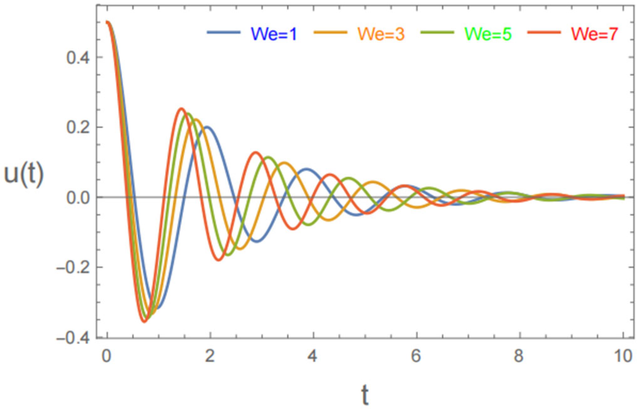
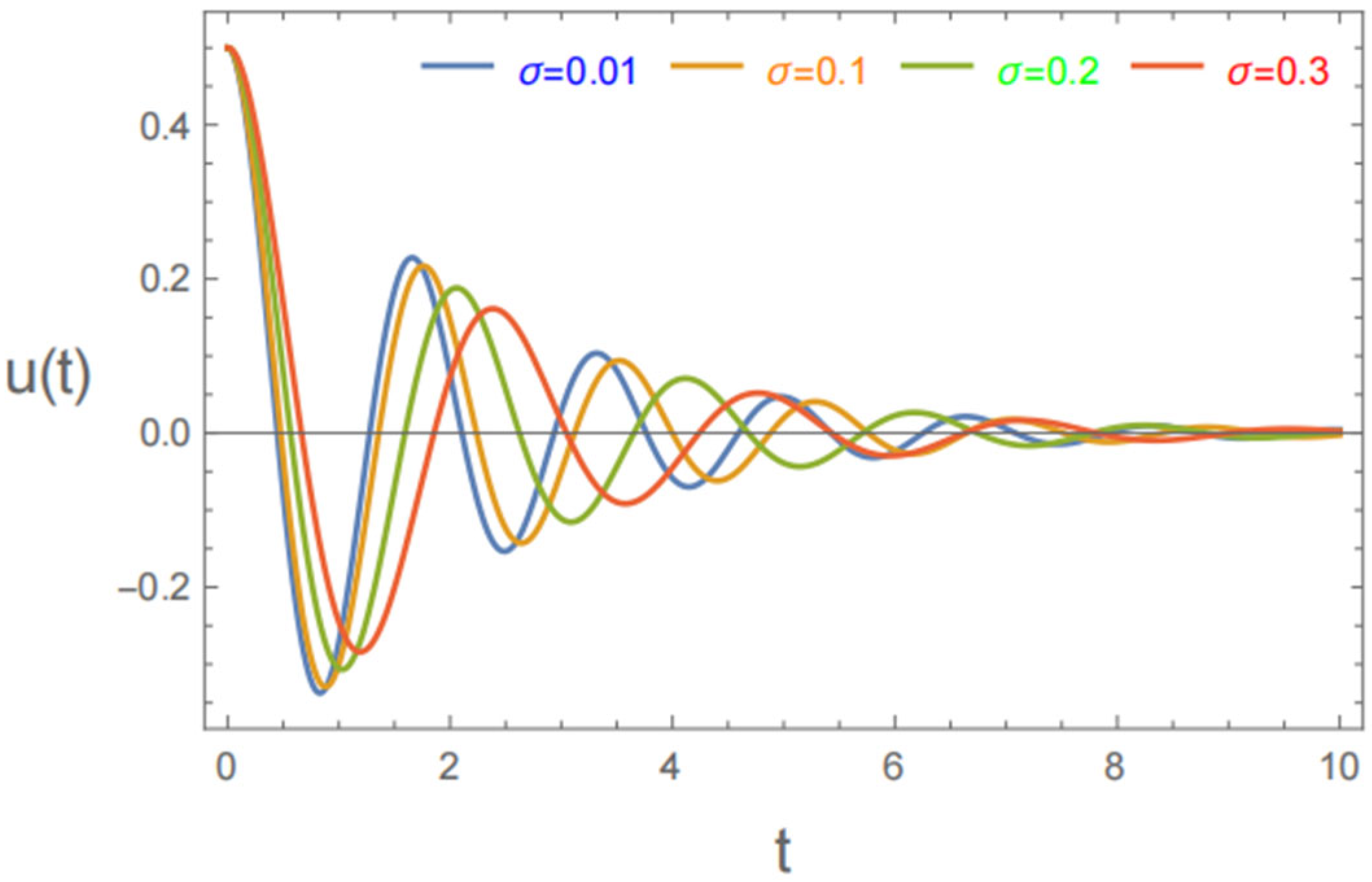
Figure 10 demonstrates the influence of the Ohnesorge number
on the instability growth rate. The Ohnesorge number represents the ratio between viscous and inertial–ST effects. This figure illustrates how increasing viscosity relative to inertia affects the development of interfacial disturbances between the two Walters’ B fluids under a periodic EF. As shown, the instability growth rate decreases with increasing
. This confirms that viscosity has a stabilizing effect by dissipating the kinetic energy of perturbations and suppressing the interface motion. Higher viscous damping reduces the amplitude of oscillations and delays the onset of instability.
Figure 11 presents the effect of the viscoelasticity factor
on the instability growth rate. This parameter characterizes the elastic relaxation property of the fluid and measures the influence of the viscoelastic stresses in the WB mode. It is evident that increasing the viscoelasticity factor leads to a reduction in the instability growth rate. This indicates that the elastic response of the fluid counteracts deformation and acts as a stabilizing mechanism. Higher viscoelastic effects delay the transmission of stress and suppress the amplification of interfacial waves.
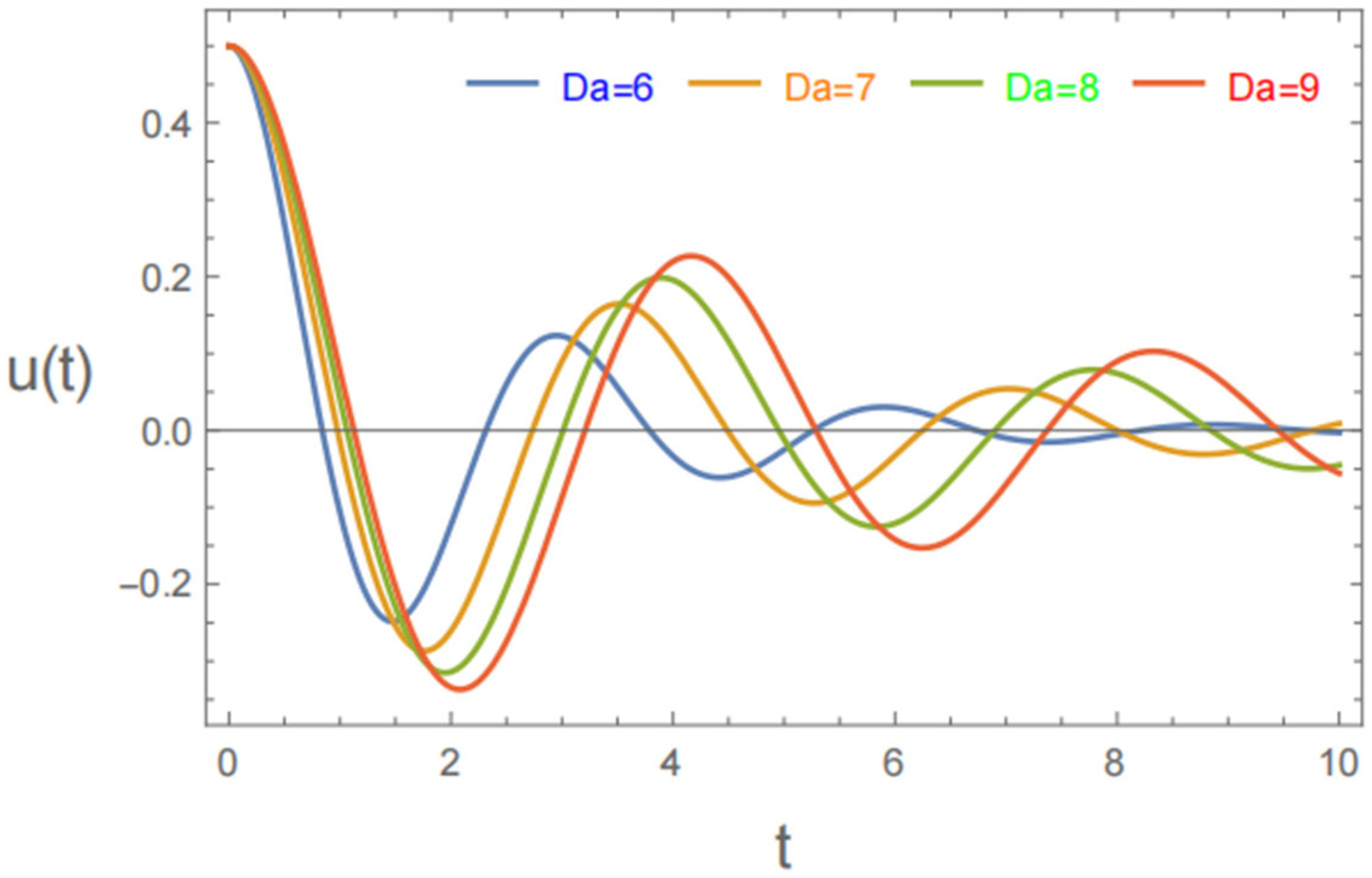
Figure 12 illustrates the effect of the Darcy number
on the instability growth rate of the two fluids through a porous medium. The
measures the permeability of the medium and reflects how easily the fluid flows through the porous structure. As seen, the instability growth rate decreases with decreasing
. A lower
corresponds to lower permeability, which increases viscous drag and energy dissipation in the porous medium, thereby stabilizing the interface. Conversely, higher permeability allows greater motion and promotes instability.
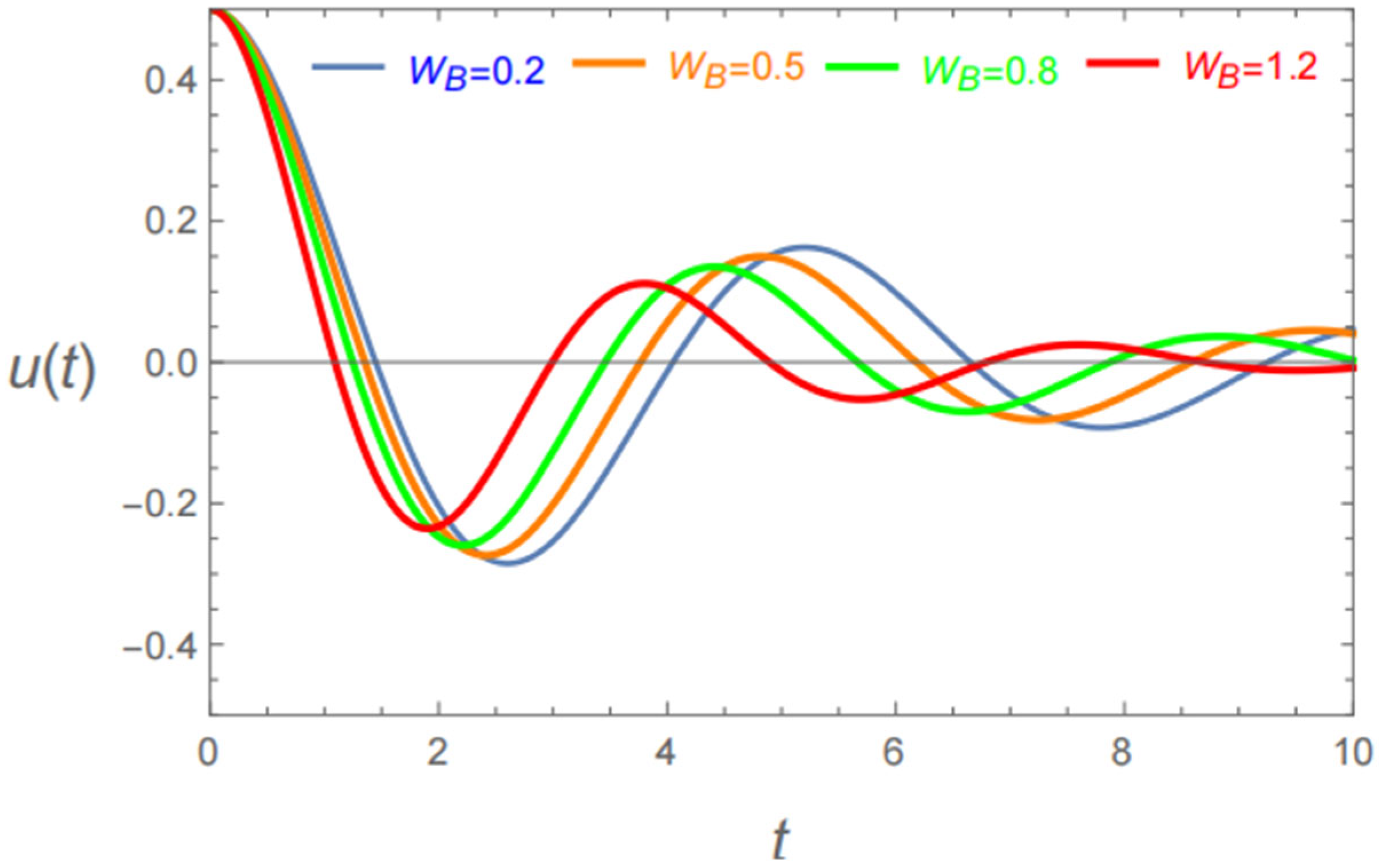
Figure 13 shows the variation in the instability growth rate with the Weber number
. The
expresses the ratio of inertial forces to ST, indicating the balance between destabilizing and stabilizing effects at the interface. It is clear that the instability growth rate increases with increasing
. Larger
enhances inertial dominance, weakening the ST restoring force and amplifying perturbations. Accordingly, inertia acts as a destabilizing factor in the system.
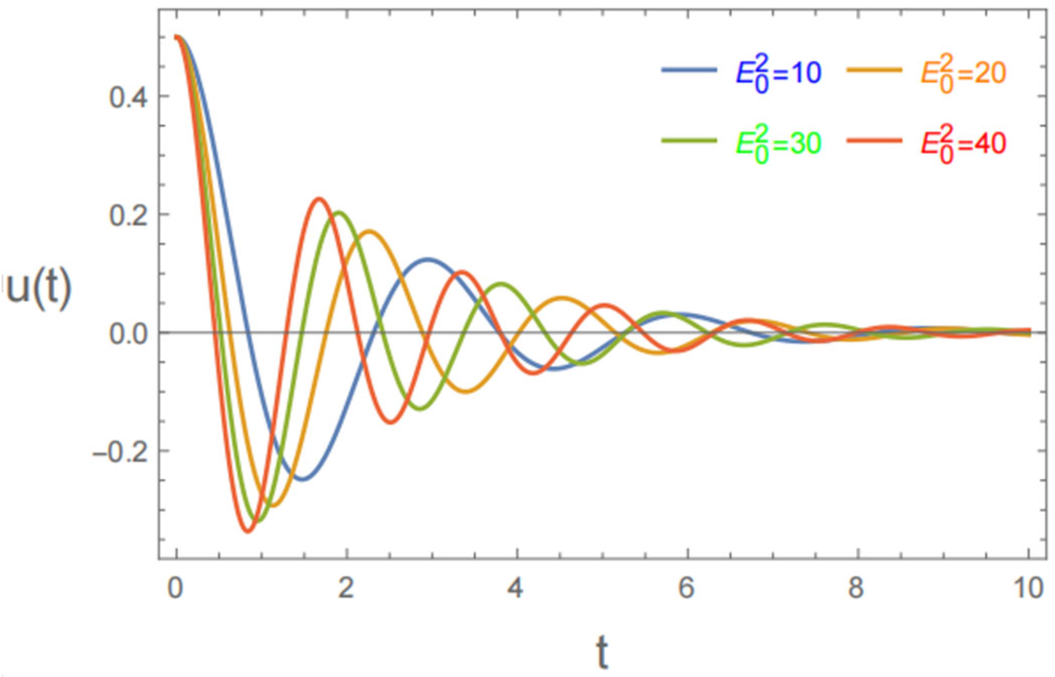
Figure 14 displays the influence of the EF parameter
on the instability growth rate. The applied EF modifies the pressure distribution along the interface due to electrostatic stresses, altering the interfacial balance between the two fluids. As observed, the instability growth rate increases as the EF strength increases. This occurs because a stronger EF enhances the electrostatic pressure difference, intensifying interfacial deformation and promoting instability.
Figure 15 depicts the variation in the instability growth rate with the frequency of the periodic EF
. This parameter controls the oscillatory nature of the electric excitation applied across the interface. It can be seen that increasing the frequency of the periodic EF affects the stability threshold of the interface. At lower frequencies, the EF acts effectively over longer times, enhancing instability; meanwhile, higher frequencies reduce its influence, leading to partial stabilization of the system.
However,
Figure 16,
Figure 17,
Figure 18 and
Figure 19 show how stability behaves. It is important to look at the stability of the resulting solution, which shows the shape of the vibration wave. The stability conditions as given in Equation (67) for a system are shown as
and
EF intensity
vs.
stability graphs are illustrated in
Figure 8,
Figure 9 and
Figure 10. For more efficacy, these profiles are shown for a few average values of the previously listed pertinent parameters, which are adjusted for each diagram based on the challenged component.
As shown in
Figure 16, the results indicate a clear dependence of the instability growth rate on the Darcy number
. A reduction in is accompanied by a noticeable decrease in the growth rate, reflecting a more stable interfacial configuration. Physically, smaller values of correspond to lower permeability of the porous structure, which imposes stronger resistance to the fluid motion. This enhanced resistance intensifies viscous losses within the porous matrix and weakens the amplification of interfacial perturbations, thereby suppressing the development of unstable modes. As a consequence, the porous layer acts as an effective stabilizing mechanism in the considered EHD configuration. In contrast, increasing
implies higher permeability and weaker drag exerted by the porous medium on the flow. Under such conditions, the fluid experiences less attenuation while moving through the porous structure, which facilitates momentum transfer across the interface and promotes the growth of disturbances driven by the electric field. The interface therefore becomes more susceptible to destabilization as
increases. This trend highlights the competing roles of viscous damping induced by the porous matrix and the destabilizing EHD forcing. Overall, the observed behavior is consistent with the physical understanding of EHD flows in porous environments, where permeability serves as a key control parameter governing the balance between stabilization due to drag and destabilization due to interfacial forcing [
21].
Figure 17 presents the influence of the viscoelasticity factor on the instability behavior of the interface between the two WB. This parameter reflects the elastic contribution of the fluid structure, which modifies the balance between stabilizing and destabilizing mechanisms in the presence of a periodic EF. As illustrated, increasing the viscoelasticity factor leads to a noticeable reduction in the instability growth rate. The presence of stronger elastic effects introduces an additional restoring force that resists deformation of the interface and suppresses the development of perturbations. Therefore, the system becomes more stable as the viscoelastic contributions increase. This behavior highlights the stabilizing role of elasticity in WB fluids and aligns with the expected rheological response of viscoelastic media subjected to interfacial disturbances [
38].
In
Figure 18, the findings investigate the function of the Weber number
. The interfacial instability between the two WB layers is under our control. It is a crucial parameter in determining the propensity of interfacial disturbances to either increase or be damped since we estimate the relative strength of inertial forces compared to ST effects. Stronger inertial contributions encourage the amplification of disturbances at the interface, as shown by the provided graphs, which show that the instability growth rate grows monotonically with increasing
. At a comparatively low level, ST acts as an efficient restorative mechanism that prevents interfacial deformation and inhibits the emergence of unstable modes.
In these circumstances, the interface stays rather steady, and disturbances are quickly smoothed off. As the ability of capillary forces to resist interfacial distortions diminishes, ST’s stabilizing effect diminishes in relation to inertia. Therefore, perturbations increase more quickly, and the contact is more susceptible to deformation. From a physical perspective, higher
facilitates the stretching and bending of the interface under EHD pressure by improving the transfer of momentum across the interface. A wider unstable zone and a faster rate of interfacial mode expansion result from this. In addition to confirming that decreasing capillary effects in comparison to inertia considerably accelerates the beginning and development of interfacial instability in the studied system, the observed trend emphasizes the critical role that surface tension plays in stabilizing the interface [
38].
In
Figure 19, the stability map shows how the density parameter significantly affects the stable and unstable zones
. The stability border shifts downward over the whole wave number
range as
grows from 0.5 to 3, suggesting that lower values of the critical EF intensity
are enough to destabilize the interface. This pattern suggests that increased density encourages the development of instability and, hence, has a destabilizing effect on the dynamics of the system. Because lighter fluids have a lesser contribution from inertia, the stable zone takes up a larger area of the parameter space for small values of
. On the other hand, rising
increases the system’s effective inertia, which lessens the capacity of stabilizing mechanisms to suppress interfacial disturbances. Density has a particularly visible effect at small and intermediate wavenumbers, where the stability curves are more widely separated. At bigger
, however, the curves gradually converge, indicating that short-wavelength modes are less sensitive to changes in
. Physically, a higher density expands the unstable domain at the expense of the stable one by increasing the momentum of the fluid layers and promoting the formation of electrically induced disturbances at the interface. According to these findings, density plays a crucial role in regulating the interfacial stability properties of the current EHD setup [
33].