A Multi-Stage Decomposition and Hybrid Statistical Framework for Time Series Forecasting

Abstract

Modeling and forecasting nonstationary and nonlinear economic time series remain fundamentally challenging due to structural breaks, volatility clustering, and noise contamination that distort the intrinsic stochastic structure. To address these limitations, this study proposes a novel three-stage hybrid statistical framework that systematically integrates multi-level signal decomposition with structured parametric modeling to enhance predictive accuracy. The proposed hybrid architectures—EMD–EEMD–ARIMA, EMD–EEMD–GMDH, and EMD–EEMD–ETS—employ a hierarchical decomposition–reconstruction strategy before forecasting. In the first stage, Empirical Mode Decomposition (EMD) decomposes the observed series into intrinsic mode functions (IMFs) and a residual component. In the second stage, Ensemble Empirical Mode Decomposition (EEMD) is applied to further refine the extracted components, mitigating mode mixing and improving signal separability. In the final stage, each reconstructed component is modeled using ARIMA, Exponential Smoothing State Space (ETS), and Group Method of Data Handling (GMDH) frameworks, and the individual forecasts are aggregated to obtain the final prediction. Empirical evaluation based on a recursive one-step-ahead forecasting scheme demonstrates consistent numerical improvements across all standard accuracy measures. In particular, the proposed EMD–EEMD–ARIMA model achieves the lowest forecasting error, reducing the root-mean-square error (RMSE) by approximately 6–7% relative to the best-performing single-stage model and by about 3–4% relative to the two-stage EMD-based hybrids. Similar improvements are observed in mean squared error (MSE), mean absolute error (MAE), and mean absolute percentage error (MAPE), indicating enhanced stability and robustness of the three-stage architecture. The results provide strong numerical evidence that multi-level decomposition combined with structured statistical modeling yields superior predictive performance for complex nonlinear and nonstationary time series. The proposed framework offers a mathematically coherent, computationally tractable, and systematically structured hybrid modeling strategy that effectively integrates noise-assisted decomposition with parametric and data-driven forecasting techniques.

1. Introduction

Modeling and forecasting macroeconomic time series remain central problems in applied statistics and mathematical modeling, particularly when the data exhibit nonstationarity, nonlinear dynamics, volatility clustering, and structural breaks [1,2,3,4,5]. Import expenditure is a critical macroeconomic indicator that directly influences gross domestic product (GDP), foreign exchange reserves, and the balance of payments. Since imports represent an outflow of domestic capital, persistent growth in import expenditure may impose pressure on macroeconomic stability [6,7,8,9,10]. From a statistical perspective, understanding the stochastic structure of import expenditure is essential for identifying trends, seasonality, and regime-dependent variations [11,12,13,14,15].

Economic time series often exhibit mixed linear and nonlinear behavior, making conventional linear models insufficient for capturing complex temporal dependencies [16,17,18,19,20]. In this context, rigorous assessment of linearity, structural variation, and signal irregularity becomes necessary. The development of advanced statistical methodologies capable of handling noisy and nonstationary processes is therefore of substantial interest [21,22,23,24,25].

The Autoregressive Integrated Moving Average (ARIMA) framework has been widely applied to univariate time-series forecasting [26,27,28]. For example, ref. [29] employed an ARIMA model to forecast gold prices and selected ARIMA(1,1,1) based on goodness-of-fit criteria. While ARIMA effectively captures short-run linear dependencies, its structure assumes linearity and may struggle to represent nonlinear patterns or sudden structural changes. Classical econometric frameworks such as ARIMA and ETS are effective models for capturing linear dependence and volatility clustering; however, they are ineffective for nonlinear dynamics and regime shifts common in real-world data [30,31]. Compared to them, machine learning approaches, like Support Vector Machines and Long Short-Term Memory networks, and hybrid neural architectures are adept at capturing nonlinearities [32,33,34,35,36]. However, these approaches typically require large datasets, often suffer from overfitting in small-sample settings, are poorly interpretable, and exhibit heterogeneous market performance across different market environments [37,38,39,40,41]. For example, ANNs often suffer from overfitting, and SVMs are usually sensitive to parameter selection [42]. In contrast, decomposition-based statistical models offer greater interpretability and robustness for nonlinear and nonstationary economic data, particularly in policy-relevant contexts [43,44,45,46,47]. Hybrid statistical frameworks have demonstrated improved forecasting performance by combining complementary modeling structures [48,49,50,51,52,53]. For instance, ref. [54] proposed a hybrid model integrating Exponential Smoothing State Space (ETS) with Artificial Neural Networks (ANN), showing superior performance relative to single models. Similarly, ref. [55] applied ARIMA to forecast COVID-19 spread dynamics, highlighting the importance of statistical modeling for capturing evolving processes and emphasizing its limitations under rapidly changing conditions.

Signal decomposition techniques have emerged as powerful mathematical tools for analyzing nonlinear and nonstationary time series [56,57,58,59,60]. Empirical Mode Decomposition (EMD), proposed by [61], decomposes a signal into intrinsic mode functions (IMFs), allowing multi-scale representation of temporal dynamics [62]. Ref. [63] integrated EMD with the Group Method of Data Handling (GMDH) to enhance forecasting accuracy. However, classical EMD suffers from the mode-mixing problem. To address this limitation, ref. [64] introduced Ensemble Empirical Mode Decomposition (EEMD), which incorporates noise-assisted data analysis to improve signal separability. Comparative investigations by [65] confirmed that EEMD more effectively mitigates mode mixing than EMD. Furthermore, hybrid EEMD-based forecasting models have demonstrated superior performance in hydrological and engineering applications [66,67,68,69,70]. However, the work in ref. [71] coupled EMD with SVM models for monthly streamflow forecasting. In [72], the authors combined three preprocessing techniques—wavelet analysis (WA), EMD, and singular spectrum analysis (SSA)—with an autoregressive moving average (ARMA) model to develop three hybrid models, WA-ARMA, EMD-ARMA, and SSA-ARMA, for monthly streamflow forecasting of two stations. The best MAPEs of these hybrid methods for the first and second stations are 34% and 26%, respectively, which are lower than the EEMD-ARIMA methods proposed by [73], which achieve an MAPE of 14.5%. That indicates EEMD is superior to EMD when examining the detailed data characteristics.

Despite these advancements, limited research has systematically explored multi-stage hybrid architectures that sequentially integrate EMD and EEMD prior to parametric modeling for macroeconomic forecasting. Import expenditure in Pakistan exhibits evolving structural characteristics influenced by exchange rate fluctuations, commodity price variability, and policy interventions. Such dynamics necessitate robust decomposition-based frameworks that isolate stochastic components prior to forecasting.

Motivated by these considerations, this study develops a structured hybrid modeling framework for forecasting import expenditure in Pakistan. The proposed methodology integrates multi-level signal decomposition with statistical forecasting models to enhance predictive accuracy. Specifically, decomposition techniques are combined with parametric and data-driven forecasting approaches, and the performance of classical univariate models, two-stage hybrids, and the proposed three-stage models is evaluated using standard forecast accuracy metrics. By systematically integrating decomposition theory with statistical time series modeling, this work contributes to recent applications of mathematical and statistical models in macroeconomic forecasting, offering a computationally efficient and structurally coherent framework for analyzing complex nonstationary economic processes.

Justification of Sequential EMD–EEMD Framework

The proposed approach employs a sequential decomposition strategy combining EMD and EEMD rather than relying solely on a single decomposition method. While EEMD and its variants (e.g., CEEMDAN) are effective in mitigating mode-mixing, applying EMD as an initial step allows for the extraction of the primary intrinsic mode functions and underlying structure of the original series. Subsequently, EEMD is applied to further refine these components through noise-assisted decomposition, thereby improving signal separability and stability. This two-stage decomposition enhances the quality of reconstructed signals by reducing noise and irregular fluctuations more effectively than using EEMD alone. Therefore, the sequential EMD–EEMD framework is designed to exploit the complementary strengths of both techniques, thereby providing a more robust representation of nonlinear and nonstationary time series for forecasting purposes.

2. Methodology

This study develops a mathematically structured three-stage hybrid forecasting framework designed for nonlinear and nonstationary univariate time series. Many economic and financial processes exhibit structural breaks, volatility clustering, heterogeneous oscillatory modes, and stochastic disturbances operating at multiple temporal scales. Such properties violate the assumptions of classical linear models and necessitate adaptive decomposition combined with flexible parametric and nonlinear modeling strategies. The proposed methodology integrates Empirical Mode Decomposition (EMD), Ensemble Empirical Mode Decomposition (EEMD), and complementary forecasting models within a coherent hierarchical architecture. The data description and empirical characteristics are presented in the subsequent section.

Let ${\left\{y_t\right\}}_{t=1}^N$ denote a univariate time series of length N. Suppose that $y_t$ is generated by a nonlinear stochastic process exhibiting mixed-frequency dynamics. The central methodological objective is to construct a forecasting operator $\mathcal{F}(·)$ such that

$${\widehat{y}}_{t+h}=\mathcal{F}(y_1,\dots ,y_t),$$

(1)

for forecast horizon $h\ge 1$, while minimizing a suitable loss function (e.g., squared error loss). The proposed solution proceeds through three mathematically motivated stages: adaptive decomposition, ensemble refinement, and predictive modeling.

2.1. Autoregressive Integrated Moving Average Model

The Autoregressive Integrated Moving Average (ARIMA) framework, introduced by Box and Jenkins [74], provides a linear stochastic representation for difference-stationary processes. After applying d-order differencing to remove stochastic trends, the transformed process satisfies

$$\mathrm{\Phi }\left(L\right){(1-L)}^d{y}_t=\mathrm{\Theta }\left(L\right){\epsilon }_t,$$

(2)

where L denotes the lag operator, $\mathrm{\Phi }\left(L\right)=1-{\varphi }_{1}L-\cdots -{\varphi }_p{L}^p$ and $\mathrm{\Theta }\left(L\right)=1+{\theta }_{1}L+\cdots +{\theta }_q{L}^q$ are autoregressive and moving average polynomials of orders p and q, and $\left\{{\epsilon }_t\right\}$ is a white noise process with zero mean and variance ${\sigma }^2$.

Equivalently,

$$y_t=a_0+\sum _{i=1}^p{a}_i{y}_{t-i}+\sum _{j=1}^q{b}_j{\epsilon }_{t-j}.$$

(3)

Model identification relies on the autocorrelation and partial autocorrelation structures, while estimation is typically performed via maximum likelihood [29,75,76]. Although ARIMA is optimal under linear Gaussian assumptions, its explanatory power diminishes when nonlinear and multi-scale effects dominate.

2.2. Exponential Smoothing State Space Model

The Exponential Smoothing State Space (ETS) framework, originally proposed by Brown [77] and formalized in state-space form by Hyndman and Khandakar [78], represents time series dynamics via recursive updating equations. A general ETS model can be expressed as

$$\begin{array}{cc}\hfill y_t& =w\left(x_{t-1}\right)+r\left(x_{t-1}\right){\epsilon }_t,\hfill \end{array}$$

(4)

$$\begin{array}{cc}\hfill x_t& =f\left(x_{t-1}\right)+g\left(x_{t-1}\right){\epsilon }_t,\hfill \end{array}$$

(5)

where ${\mathbf{x}}_t$ denotes the state vector containing level, trend, and seasonal components, and ${\epsilon }_t\sim \mathcal{N}(0,{\sigma }^2)$. Additive error models satisfy $y_t={\mu }_t+{\epsilon }_t$, whereas multiplicative error models take the form $y_t={\mu }_t(1+{\epsilon }_t)$.

The ETS taxonomy classifies models according to error, trend, and seasonality components, yielding a finite set of stochastic specifications. Maximum likelihood estimation ensures statistical consistency and facilitates probabilistic forecasting.

2.3. Group Method of Data Handling

To capture nonlinear dependencies, the Group Method of Data Handling (GMDH), introduced by Ivakhnenko [79], is incorporated. GMDH constructs layered polynomial networks that approximate nonlinear functional relationships among lagged inputs. For two input variables $(x_i,x_j)$ selected from lagged observations, a typical neuron takes the quadratic form

$${\widehat{y}}_t=a_0+a_1{x}_i+a_2{x}_j+a_3{x}_i^2+a_4{x}_j^2+a_5{x}_i{x}_j.$$

(6)

Through iterative layer construction and external validation-based selection, the network self-organizes to minimize forecasting error [54,80,81,82]. This structure enables flexible approximation while mitigating overfitting.

2.4. Empirical Mode Decomposition

Empirical Mode Decomposition (EMD), introduced by Huang et al. [61], provides an adaptive, data-driven method for decomposing nonlinear and nonstationary signals into intrinsic mode functions (IMFs). Each IMF satisfies two mathematical conditions: (i) the number of extrema and zero crossings differs at most by one; (ii) the mean of the upper and lower envelopes equals zero at each point [83,84].

Through iterative sifting, the signal can be expressed as

$$y_t=\sum _{k=1}^K{\mathrm{IMF}}_{k,t}+h_t,$$

(7)

where $h_t$ represents the residual trend component. EMD acts as an adaptive filter bank separating oscillatory modes across distinct time scales [85,86,87,88]. However, classical EMD may suffer from mode mixing.

2.5. Ensemble Empirical Mode Decomposition

Ensemble Empirical Mode Decomposition (EEMD) extends EMD by introducing white noise perturbations and ensemble averaging to mitigate mode mixing [89,90]. For each ensemble realization $m=1,\dots ,M$, a noise-assisted signal is generated:

$$y_t^{\left(m\right)}=y_t+\alpha {\sigma }_y{\epsilon }_t^{\left(m\right)},$$

(8)

where ${\epsilon }_t^{\left(m\right)}\sim \mathcal{N}(0,1)$ and $\alpha$ controls the noise amplitude. Applying EMD to each realization yields

$$y_t^{\left(m\right)}=\sum _{i=1}^K{k}_{i,t}^{\left(m\right)}+h_t^{\left(m\right)}.$$

(9)

The final IMFs are obtained via ensemble averaging,

$$k_{i,t}={\displaystyle \frac{1}{M}}\sum _{m=1}^M{k}_{i,t}^{\left(m\right)},$$

(10)

and similarly for the residual. This ensemble mechanism improves statistical stability and scale separation.

2.6. Intrinsic Mode Functions

The main step in selecting IMFs is to identify oscillations in a signal from a local time scale [83]. The IMFs are obtained from the data and serve as the origin of the extension, which can be linear or non-linear, as determined by the data. Two conditions have been satisfied by IMFs, showing the numerous intrinsic time scales of the data, which include the number of extrema and the number of zero crossings, essentially either equivalent or dissimilar at most by one, and the mean value of the case determined by the local extremity and local minima is zero at any specified point. IMF contains the highest frequency, while residual contains the lowest frequency [85]. IMFs serve as a filter bank and are an important tool for noise reduction.

Steps of Decomposition into Intrinsic Mode Functions

The following steps are involved in decomposing a signal into an intrinsic mode functions (IMFs):

• Identify all local maxima and local minima of the signal $y_t$.
• Construct the upper envelope $z_t$ by interpolating the local maxima and the lower envelope $w_t$ by interpolating the local minima using cubic spline interpolation.
• Compute the mean of the upper and lower envelopes

  $$n_t={\displaystyle \frac{z_t+w_t}{2}}$$

  (11)
• Obtain the first detail component by subtracting the mean envelope from the original signal:

  $$d_{1,t}=y_t-n_t$$

  (12)
• Repeat Steps 1–4 on the detail signal $d_{k,t}$ until the resulting signal satisfies the IMF conditions. The extracted signal is defined as the first IMF:

  $${\mathrm{IMF}}_{1,t}=d_{1,t}$$

  (13)
• Subtract the extracted IMF from the signal to obtain the residual:

  $$h_{1,t}=y_t-{\mathrm{IMF}}_{1,t}$$

  (14)
• Repeat the above procedure on successive residuals until no further IMFs can be extracted.

Accordingly, the original signal can be expressed as:

$$y_t=\sum _{k=1}^K{\mathrm{IMF}}_{k,t}+h_t,$$

(15)

where K is the number of extracted IMFs and $h_t$ denotes the final residual.

2.7. Proposed Three-Stage Hybrid Framework

The proposed hybrid framework integrates EMD, EEMD, and forecasting models within a unified decomposition–estimation paradigm. The proposed models are designed to forecast non-stationary time-series data. In Stage 1, EMD is applied to the original series $y_t$ to decompose it into K intrinsic mode functions (IMFs) and a residual component. The decomposition is performed using Sifting iterations $S=60$ and $num\_sifting=50$. This decomposition yields 6 IMFs, denoted $k_{1,t}, k_{2,t}, \dots , k_{6,t}$, and a residual $h_t$, such that:

$$y_t=\sum _{i=1}^6{k}_{i,t}+h_t$$

(16)

To reduce high-frequency noise, MAD-based soft thresholding is applied to the IMFs, defined as:

$$T_i=0.6\sqrt{2\mathrm{MAD}\left(k_{i,t}\right)·log\left(N\right)},i=1,2,\dots ,6$$

(17)

where $N=144$ is the length of the series. The scaling factor (0.6) used in the thresholding function follows common practices in signal denoising literature and was selected to balance noise reduction and signal preservation.

The denoised IMFs and the residual $h_t$, are recombined to obtain the reconstructed EMD signal:

$$y_t^{\left(\mathrm{EMD}\right)}=\sum _{i=1}^6{k}_{i,t}^{\mathrm{denoised}}+h_t$$

(18)

$IM{F}_1$, $IM{F}_2$ capture high-frequency noise or short-term fluctuations, $IM{F}_3$ and $IM{F}_4$ capture medium-frequency components, which are often related to cyclical patterns, and $IM{F}_5$, $IM{F}_6$ capture lower-frequency, long-term cycles. Residual $h_t$ represents the underlying long-term trend.

In Stage 2, EEMD is applied to the reconstructed signal $y_t^{\left(\mathrm{EMD}\right)}$ to address mode mixing and refine the decomposition. EEMD is performed with an ensemble size of M = 13,000, noise strength set to $\alpha =2.5$, Sifting iterations $S=60$, and $num\_sifting=50$. The decomposition yields six EEMD-based IMFs, denoted $k_{1,t}^{\left(E\right)}, k_{2,t}^{\left(E\right)}, \dots , k_{6,t}^{\left(E\right)}$, and a residual $h_t^{\left(E\right)}$.

The MAD-based soft thresholding is applied to the IMFs, and the final denoised signal is reconstructed as:

$$y_t^{\left(\mathrm{EEMD}\right)}=\sum _{i=1}^6{k}_{i,t}^{(E,\mathrm{denoised})}+h_t^{\left(E\right)}$$

(19)

The resulting signal $y_t^{\left(\mathrm{EEMD}\right)}$ is smoother, denoised, and free from mode mixing, making it well-suited for subsequent forecasting models.

In Stage 3, the denoised signal $y_t^{\left(\mathrm{EEMD}\right)}$ is modeled using ARIMA, ETS, and GMDH within a recursive forecasting scheme. For each forecast origin t, the model is estimated using available observations and produces a one-step-ahead forecast ${\widehat{y}}_{t+1}$. Forecast performance is evaluated using error-based criteria, such as the root-mean-square error.

Theoretically, the proposed EMD–EEMD–Model structure operationalizes the principle of multi-resolution decomposition. The first two stages act as variance-reduction and frequency-localization operators, transforming a complex nonlinear stochastic process into quasi-stationary subcomponents. The final stage exploits complementary linear and nonlinear approximators to capture remaining dependencies. This hierarchical integration enhances robustness, reduces the risk of model misspecification, and provides a mathematically consistent framework aligned with recent applications of statistical and mathematical models to complex time-series forecasting.

2.8. Hyperparameter Specification

The performance of the proposed framework depends on several key hyperparameters. In the EEMD procedure, the ensemble size is set to $M=\mathrm{13,000}$, and the noise amplitude is set to $\alpha =2.5$; these are selected to ensure stable decomposition and effective noise-assisted signal separation.

In the thresholding function, a scaling constant of 0.6 is employed. This value follows common practices in the signal denoising literature and provides a balance between noise reduction and preservation of important signal characteristics.

These parameter choices are selected to enhance decomposition stability and forecasting performance while maintaining robustness across the dataset.

Decomposition Strategy: It is important to note that both EMD and EEMD decompositions are applied globally to the full time series rather than within a rolling window framework. The forecasting procedure follows a recursive expanding-window approach, where models are re-estimated at each step using all available observations up to that point.

For EMD, parameters such as the S-number and number of siftings are explicitly specified. For EEMD, the ensemble size (M = 13,000) and noise strength ($\alpha =2.5$) are selected to ensure stable and reliable decomposition.

This global decomposition strategy avoids instability in intrinsic mode functions (IMFs) across time and ensures consistent signal representation, which is particularly important in relatively small-sample macroeconomic datasets.

2.9. Forecast Accuracy Measures

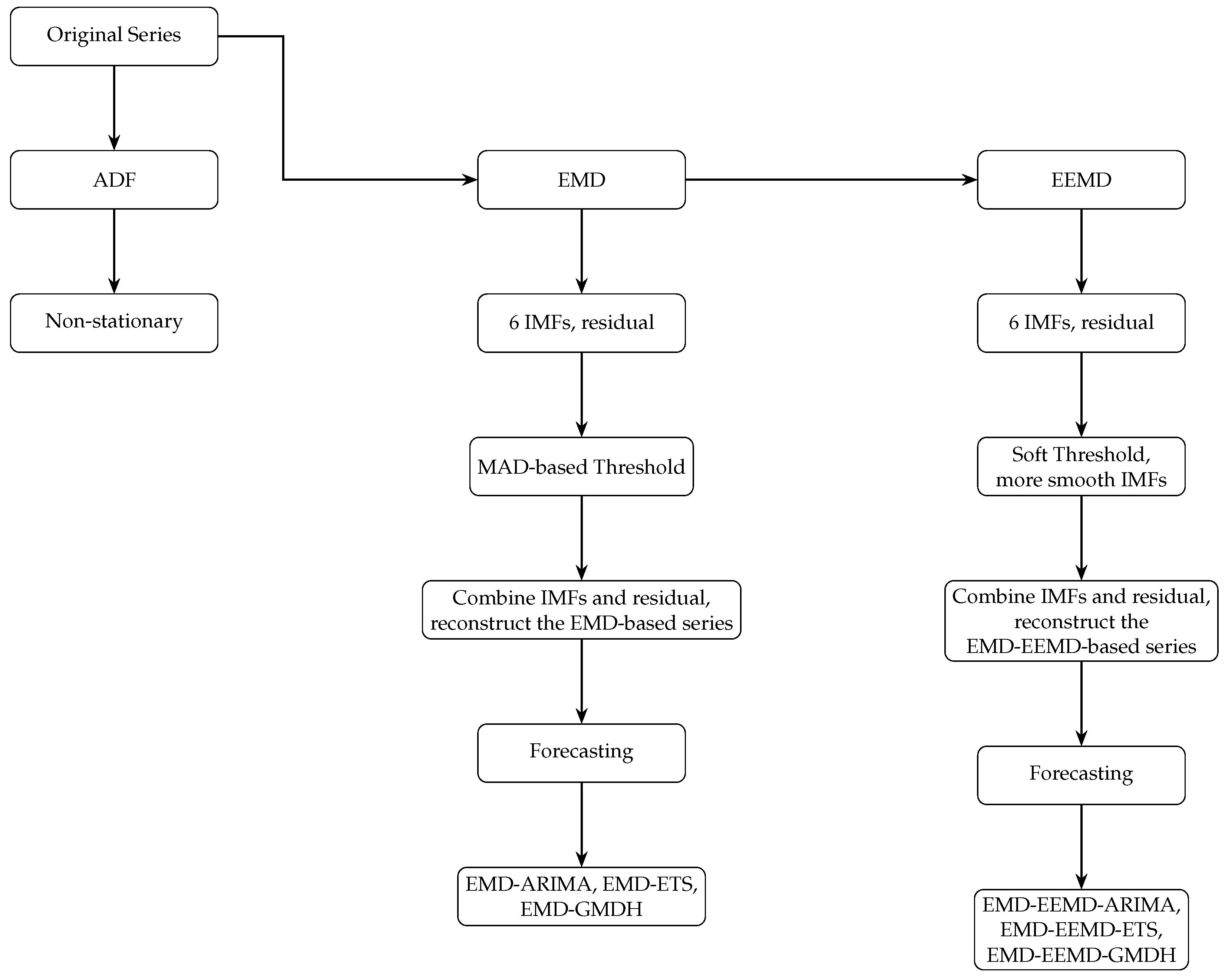
Forecasting performance of all competing models is evaluated using four widely adopted accuracy metrics: the mean squared error (MSE), root mean squared error (RMSE), mean absolute error (MAE), and mean absolute percentage error (MAPE). These criteria quantify the deviation between realized observations and their corresponding one-step-ahead forecasts over a fixed evaluation horizon. Finally, the complete layout of the proposal forecasting is shown in Figure 1.

3. Case Study Results

The study analyzes monthly import expenditure data spanning from January 2010 to December 2021. The dataset exhibits characteristics typical of economic time series, including non-stationarity, structural trends, and irregular fluctuations, which complicate accurate forecasting. To address these challenges, this study proposes three novel three-stage hybrid models designed to enhance prediction accuracy. The hybrid framework consists of three sequential stages: decomposition, forecasting, and evaluation of predictive performance. In the decomposition stage, Empirical Mode Decomposition (EMD) is employed to separate the original time series into intrinsic mode functions (IMFs) and a residual component, effectively isolating high-frequency noise from longer-term trends. Ensemble Empirical Mode Decomposition (EEMD) is subsequently applied to the EMD-based reconstructed signal to mitigate mode-mixing and produce more stable, physically meaningful components.

3.1. Study Period Justification

The study period from January 2010 to December 2021 is selected to capture both stable economic conditions and periods of significant disruption. In particular, the latter part of the sample includes the COVID-19 pandemic, which introduced substantial volatility, structural changes, and irregular fluctuations in international trade and import expenditure.

Including this period allows for a more comprehensive evaluation of the proposed forecasting framework under both normal and extreme conditions. The presence of such disruptions provides an opportunity to assess the model’s robustness to nonstationarity, noise, and regime shifts.

To account for these effects, structural break analysis has been conducted using the Chow test and CUSUM procedure, and the results are discussed in the empirical section. Furthermore, the decomposition-based structure of the proposed model enables effective separation of noise and signal components, making it suitable for handling abrupt changes and irregular patterns in economic time series.

3.2. Justification of the Final Sample Period

The inclusion of the 2020–2021 period in the dataset is motivated by two key considerations. First, it reflects the availability of the most recent observations, ensuring that the analysis is based on up-to-date economic information. Second, and more importantly, this period captures the unprecedented disruptions caused by the COVID-19 pandemic, including abrupt changes in trade flows, increased volatility, and structural shifts in economic activity. Including this period allows the proposed forecasting framework to be evaluated under both stable and extreme conditions, thereby providing a more comprehensive assessment of its robustness and adaptability. This is particularly important for macroeconomic forecasting models, which must remain reliable under unexpected shocks and regime changes.

The effectiveness of the proposed hybrid models is evaluated by comparing their forecasting performance with that of traditional univariate models and two-stage hybrid models. Unlike classical linear or single-stage approaches, which may struggle to capture the inherent non-stationarity and nonlinearities of import expenditure series, the proposed three-stage models leverage multiscale decomposition to separate distinct temporal patterns. This allows the forecasting models to focus on denoised, frequency-specific components, thereby improving their ability to track both short-term fluctuations and long-term trends. The subsequent sections present the empirical results, highlighting the performance gains achieved through this decomposition-based hybrid framework and illustrating the advantages of combining EMD, EEMD, and robust statistical forecasting methods for complex economic time series. From a modeling and forecasting perspective, the dataset is split into training and testing sets: the first eight years of observations are used for model training, while the remaining four years are reserved for out-of-sample evaluation. One-step-ahead rolling forecasting is employed, where the model is iteratively re-estimated, with each successive observation included in the training set.

Table 1. Descriptive statistics and Augmented Dickey–Fuller (ADF) test results.

Statistic	n	Minimum	Maximum	Mean	Median	S.D
Import Expenditure	144	2341.284	6430.971	3788.621	3558.503	829.27
ADF Test Results
Series	ADF Statistic		p-Value
Import Expenditure (Level)	−0.9304		0.946
Import Expenditure (1st Difference)	−4.215		0.001

exhibits the descriptive statistics and ADF test value on level (0) and level (I) to the time series of total import expenditure. The import expenditure series shows moderate variability and is non-stationary at level (p = 0.946), but becomes stationary after first differencing (p = 0.001). ARIMA, GMDH, and ETS models, which are specifically designed to handle non-stationary behavior, were applied directly to the original series used as a benchmark.

The optimal ARIMA model was selected using the auto.arima() function in R 4.5.0, which automatically determines the parameters p, d, and q by minimizing an information criterion, specifically the Akaike Information Criterion (AIC). The procedure jointly evaluates different model configurations rather than estimating separate AR and MA models independently.

The auto.arima() function was implemented using a stepwise search strategy with non-seasonal specifications, as no strong seasonal patterns were detected in the data. Stationarity was assessed internally through differencing as required by the algorithm. The resulting model configurations, including AR(3,0,0) and MA(0,0,3), are interpreted as specific ARIMA structures identified during the selection process and are reported for comparative analysis. This approach ensures a systematic and reproducible model selection process while avoiding manual specification bias.

The ETS is applied to the series. The ETS is tasked with automatically selecting a suitable model using maximum likelihood to produce forecasts for various steps ahead as required. The ETS generates the best model for our series: ETS(M, Ad, M). In ETS, this three-character string shows error, trend, and seasonality. An error can be additive or multiplicative, and a trend can be additive, additive damped, multiplicative, multiplicative damped, or none, whereas a seasonality can be additive, multiplicative, or none. It indicates multiplicative error and seasonality, with the parameter amplified over time, whereas the trend is additive and damped. Damping is the reduction of trend size over time until it approaches a straight line. There are four parameters: $\alpha , \beta , \varphi$, and $\gamma$, where $\alpha$ is the smoothing parameter for level, $\beta$ is the smoothing parameter for trend, $\varphi$ is the damping coefficient, and $\gamma$ is the smoothing factor for seasonality. Small values of $\beta$ = 0.001 and $\gamma$ = 0.001 show that both trend and seasonal components do not vary rapidly with time. The initial state includes equations for level, trend, and seasonality; i.e., $l_t$ represents the level equation, $b_t$ the trend equation, and $s_t$ the seasonal equation.

A Group Method of Data Handling (GMDH) model is applied to the original time series using the fcast() function from the GMDH package in R. The GMDH algorithm is a self-organizing approach that builds nonlinear polynomial models by automatically selecting the most relevant input features and model structure based on prediction performance. GMDH-based algorithms are used for short-term forecasting. It determines the relation among the lags of our series of total imports. GMDH differs from a well-organized forecasting method. It has valid properties that enable it to find the best solution from the possible variants. It is a set of algorithms that can be combined to solve different problems. The GMDH model was implemented with input lag = 3, single-layer architecture, and regularization parameters selected via cross-validation. The model’s performance can be measured by the imprecision between estimated and observed values in the dataset.

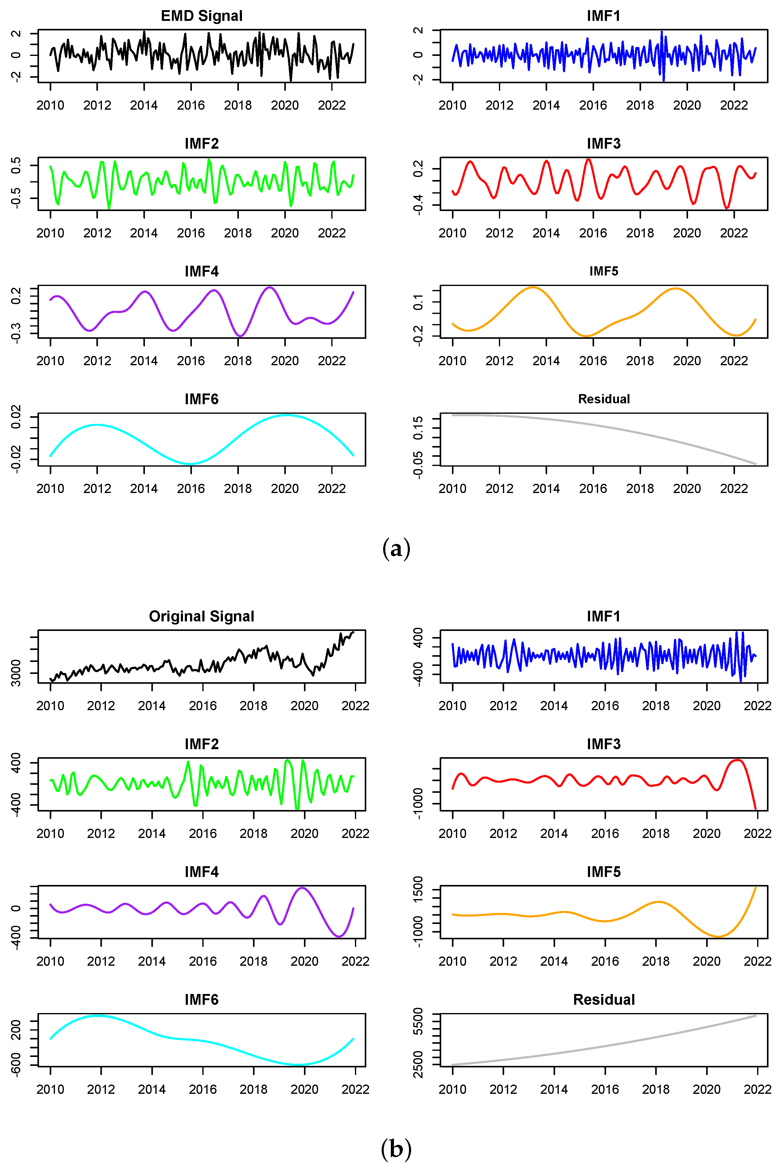
To enhance forecasting accuracy, this work employed a three-stage hybrid modeling framework that combines Empirical Mode Decomposition (EMD), Ensemble Empirical Mode Decomposition (EEMD), and conventional forecasting models. In the first stage, the original nonstationary, nonlinear series of import expenditure was decomposed using EMD into a finite set of Intrinsic Mode Functions (IMFs) and a residual component. Each IMF exhibited oscillatory behavior across distinct frequency bands, with lower-order IMFs capturing high-frequency fluctuations (noise), middle-order IMFs representing cyclical variations, and higher-order IMFs, along with the residual, preserving long-term trends. To reduce noise, soft thresholding based on the Median Absolute Deviation (MAD) was applied to the IMFs before signal reconstruction. In the second stage, the reconstructed signal from EMD was further processed with EEMD to address the mode-mixing limitation inherent in classical EMD. EEMD decomposed the denoised signal by introducing controlled white noise and averaging across multiple ensembles, thereby producing more stable and physically meaningful IMFs, as shown in Figure 2. A similar thresholding was applied to the high-frequency modes, and a final refined signal was reconstructed.

3.3. Justification of Model Selection and Benchmark Design

The primary objective of this study is to evaluate the effectiveness of the proposed hybrid decomposition framework (EMD and EEMD) in improving forecasting performance. In this context, automatic model selection using information criteria (e.g., AIC) is employed to ensure a consistent and unbiased identification of suitable model specifications, avoiding subjective tuning. The ARIMA, ETS, and GMDH models are applied directly to the original series as benchmark models. This enables a systematic comparison among single-stage (original series), two-stage (EMD-based), and three-stage (EMD–EEMD-based) forecasting approaches. Such a design enables the isolation of the contribution of decomposition techniques in enhancing forecast accuracy. In addition, standard diagnostic checks, including residual autocorrelation and white noise verification, were considered to ensure the adequacy and stability of the selected models.

3.4. Consistency with the Hybrid Architecture

The ARIMA, ETS, and GMDH models are applied directly to the original series as benchmark models. This enables a systematic comparison among single-stage (original series), two-stage (EMD-based), and three-stage (EMD–EEMD-based) forecasting approaches. By doing so, the specific contribution of the hierarchical decomposition strategy can be clearly distinguished from the inherent predictive capabilities of these classical models. Furthermore, the automatic model selection process using information criteria (e.g., AIC) is applied consistently to these benchmark models, ensuring transparency, reproducibility, and rigorous evaluation of forecast performance across different modeling stages.

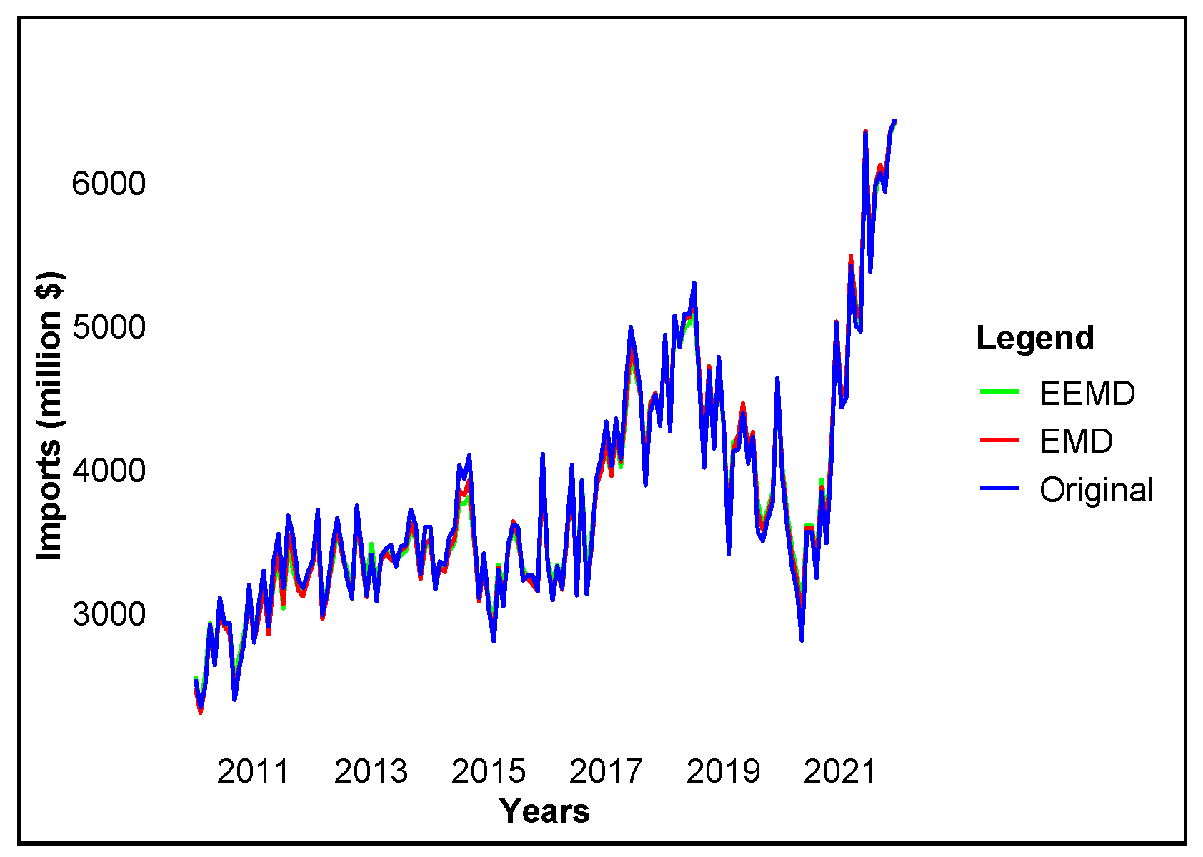
On the other hand, the plots of the EMD- and EEMD-based denoised series, compared with the original series, are shown in Figure 3.

Table 2. Performance comparison of forecasting models based on error metrics.

Model Name	Stage	MSE	RMSE	MAE	MAPE
ETS	One-stage	264763.8	514.5520	396.1403	9.1862
ARIMA	One-stage	257434.2	507.3797	390.4360	9.0748
GMDH	One-stage	278254.3	527.4981	417.8787	9.5913
EMD–ETS	Two-stage	247012.9	497.0039	384.3285	8.9328
EMD–ARIMA	Two-stage	242589.6	492.5339	382.6195	8.9003
EMD–GMDH	Two-stage	263865.8	513.6787	407.0438	9.3871
EMD–EEMD–ETS	Three-stage	248486.4	498.4841	382.5381	8.8854
EMD–EEMD–ARIMA	Three-stage	224204.2	473.5021	354.3218	8.3290
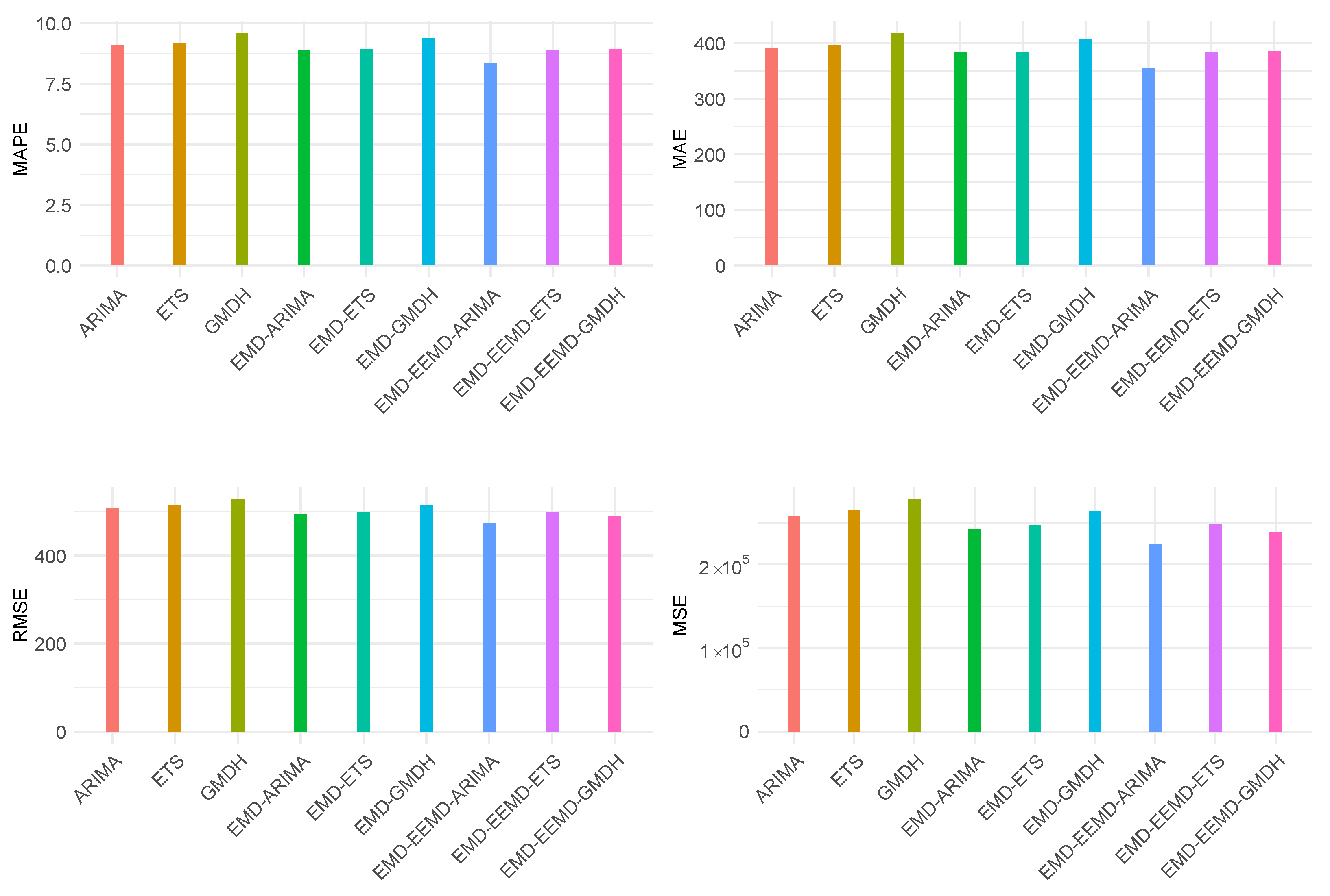
EMD–EEMD–GMDH	Three-stage	238649.3	488.5174	384.5471	8.9120

lists numerically and Figure 4 visually the out-of-sample forecasting performance of one-stage, two-stage, and three-stage models evaluated using MSE, RMSE, MAE, and MAPE over the forecasting horizon $H=48$. A clear pattern emerges across the results, indicating that decomposition-based hybrid structures systematically improve predictive accuracy relative to conventional single-stage models. However, among the one-stage models, ARIMA exhibits the best overall performance with the lowest MSE (257434.2), RMSE (507.3797), MAE (390.4360), and MAPE (9.0748) compared to ETS and GMDH. Although ETS performs competitively in terms of MAE (396.1403) and MAPE (9.1862), ARIMA provides the most consistent reduction across all error measures. On the other hand, the two-stage hybrid models based on EMD decomposition demonstrate noticeable improvements over their single-stage counterparts. In particular, the EMD–ARIMA model reduces the MSE to 242589.6 and the RMSE to 492.5339, reflecting improved modeling of multi-scale structures extracted via decomposition. Similarly, EMD–ETS achieves lower MAE (384.3285) and MAPE (8.9328) relative to the original ETS model. These results confirm that preliminary signal decomposition helps isolate intrinsic oscillatory components, thereby improving forecast stability and accuracy.

Further performance gains are observed under the three-stage framework that integrates both EMD and EEMD. The EMD–EEMD–ARIMA model clearly outperforms all competing approaches, achieving the smallest MSE (224204.2), RMSE (473.5021), MAE (354.3218), and MAPE (8.3290). This substantial reduction in forecast error suggests that the additional decomposition layer effectively mitigates residual noise and enhances the structural separation of deterministic and stochastic components. While EMD–EEMD–ETS and EMD–EEMD–GMDH also demonstrate improvements relative to two-stage models, their gains are less pronounced than those of the ARIMA-based three-stage configuration. Thus, the empirical evidence indicates a monotonic improvement in forecasting accuracy as the modeling structure evolves from single-stage to multi-stage decomposition-based hybridization. The results strongly support the superiority of the proposed three-stage hybrid framework, particularly the EMD–EEMD–ARIMA specification, in capturing nonlinear and nonstationary characteristics of the underlying time series.

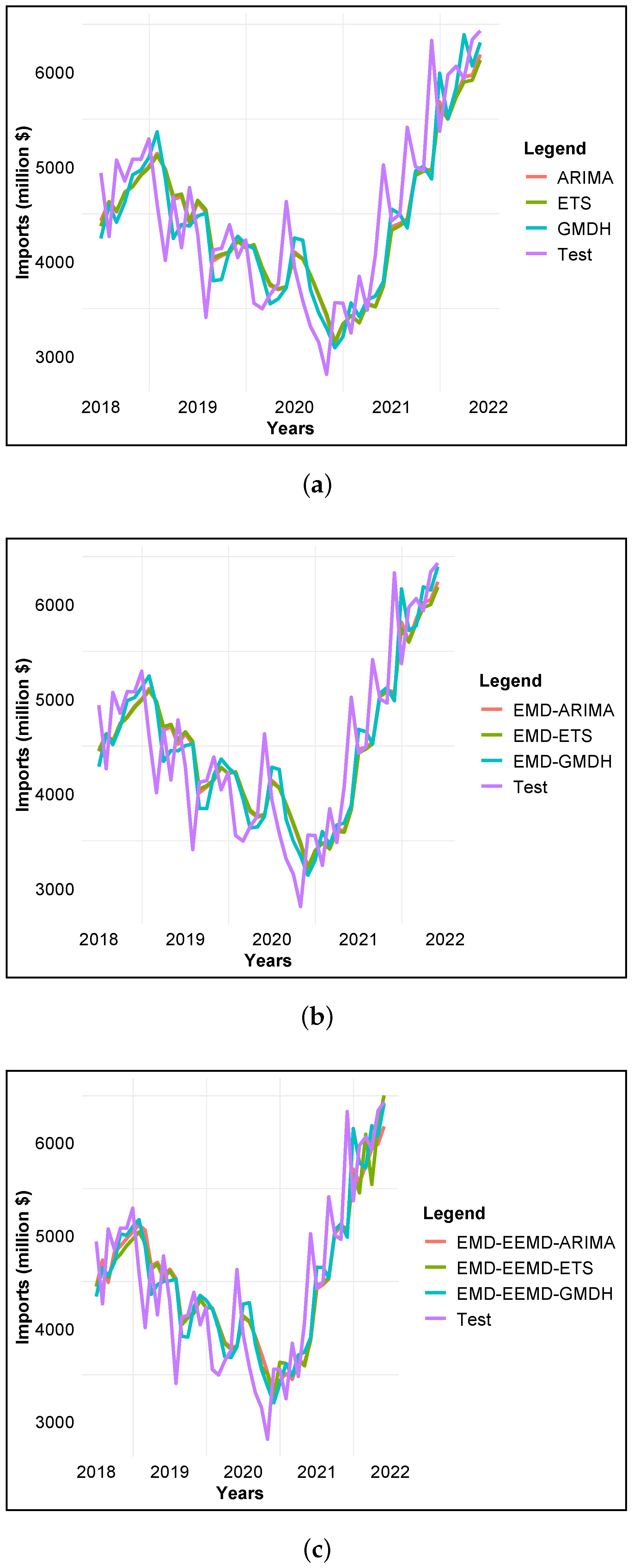
In addition to the above, Figure 5 illustrates the comparative one-step-ahead forecasting performance of the competing models under three structural configurations: (a) single-stage models; (b) two-stage decomposition-based hybrid models; (c) the proposed three-stage hybrid framework. Panel (a) presents the forecasting behavior of conventional single-stage models, namely ARIMA, ETS, and GMDH, applied directly to the original series without prior signal decomposition. While these models capture the overall trend of the observed data, noticeable deviations occur during periods of structural fluctuations and high variability. In particular, forecast trajectories exhibit lagging behavior around turning points, reflecting the limitations of purely parametric or standalone machine learning approaches in modeling multi-scale nonlinear dynamics. Panel (b) depicts the performance of the two-stage hybrid models, where empirical mode decomposition (EMD) is first employed to decompose the original series into intrinsic mode functions (IMFs) and a residual component. The forecasting models (ARIMA, ETS, and GMDH) are then applied to the reconstructed signal. Relative to the single-stage configuration, the forecasts exhibit improved alignment with the observed series, especially in capturing short-term oscillatory movements. The decomposition step effectively isolates high-frequency noise and structural components, allowing the forecasting models to operate on a smoother and more structured representation of the data. Panel (c) shows the forecasting results of the proposed three-stage hybrid framework, in which both EMD and EEMD are sequentially applied to refine the decomposition and mitigate mode-mixing effects. The ARIMA, ETS, and GMDH models are subsequently fitted to the final reconstructed signal and used to generate recursive one-step-ahead forecasts. This multi-level decomposition enhances the separation of deterministic trend, cyclical dynamics, and stochastic noise components. Consequently, the forecasts in panel (c) demonstrate superior tracking ability, reduced volatility in prediction errors, and improved responsiveness around structural shifts. Thus, the graphical evidence corroborates the quantitative findings reported in Table 2. A progressive improvement in forecasting precision is observed as the modeling architecture evolves from single-stage to two-stage and finally to the proposed three-stage hybrid structure. The results highlight the effectiveness of multi-scale signal decomposition in enhancing the predictive performance of conventional statistical and machine-learning forecasting models.

3.5. Structural Break Analysis

The out-of-sample evaluation period (2018–2021) coincides with the global COVID-19 pandemic, which significantly disrupted international trade flows and economic activity. Such an event may introduce structural breaks in the time series, potentially affecting model stability and forecast accuracy. Therefore, it is important to formally examine the presence of structural changes in the data. To address this issue, structural break tests were conducted using the Chow test and the CUSUM test. The Chow test tests for a breakpoint at a specified period, whereas the CUSUM test tests for the stability of model parameters over time. The results of these tests are presented in

Table 3. Structural break test results.

Test	Test Statistic	p-Value	Decision
Chow Test (2019 Breakpoint)	5.87	0.003	Structural Break Detected
CUSUM Test	—	—	Parameter Instability Observed

.

The Chow test results indicate a statistically significant structural break around the COVID-19 period (p-value < 0.05). In addition, the CUSUM test indicates instability in the model parameters during this period, confirming a regime shift in the data-generating process. These findings are consistent with the economic disruptions caused by the pandemic. Despite this, the proposed multi-stage hybrid framework remains robust, as the decomposition-based approach allows effective handling of nonstationary and nonlinear patterns. However, the presence of structural breaks may influence forecast performance, and results for this period should be interpreted with appropriate caution.

3.6. Impact of Exogenous Shocks

Exogenous shocks, such as the COVID-19 pandemic, can significantly alter the statistical properties of economic time series, affecting stationarity, trend behavior, and variance structure. These abrupt changes may induce regime shifts and increased volatility, posing challenges for traditional forecasting models.

In this study, such effects are addressed both explicitly and implicitly. Structural break tests (Chow and CUSUM) are employed to identify changes in the data-generating process during the pandemic period. In addition, the EMD–EEMD decomposition framework inherently captures these variations by decomposing the original series into intrinsic mode functions (IMFs) across multiple time scales.

Lower-order IMFs reflect high-frequency fluctuations and volatility, while higher-order IMFs and residual components capture long-term structural changes. This multiscale representation enables the model to adapt to nonstationarity and regime shifts induced by exogenous shocks, thereby improving forecasting robustness without relying on strict parametric assumptions.

4. Discussion

The results demonstrate that the proposed three-stage hybrid models substantially enhance the forecasting accuracy of import expenditure time series compared to single- and two-stage approaches. While single-stage models (ARIMA, ETS, GMDH) capture linear trends and short-term autocorrelations, their predictive performance is constrained by high-frequency fluctuations and irregular noise inherent in the raw series. Two-stage models incorporating Empirical Mode Decomposition (EMD) improve forecasts by isolating intrinsic mode functions (IMFs) corresponding to different frequency components and applying thresholding to reduce noise. This decomposition allows subsequent forecasting models to focus on more stable, structured signals, resulting in improved accuracy, particularly for EMD-ARIMA.

The three-stage framework, which integrates Ensemble Empirical Mode Decomposition (EEMD), further refines this process by mitigating mode-mixing through noise-assisted decomposition. By averaging IMFs across multiple realizations with added noise, EEMD produces more physically interpretable and smoother components, preserving essential long-term trends while attenuating high-frequency irregularities. Forecasting models applied to these EEMD-processed series leverage this improved signal separation, leading to the observed superior accuracy. The multiscale decomposition effectively separates noise from signal across temporal scales: lower-order IMFs capture high-frequency fluctuations, intermediate IMFs reflect cyclical dynamics, and higher-order IMFs, along with the residual, encode long-term trends. This aligns with broader findings in the hybrid forecasting literature, which suggest that sequential decomposition combined with robust statistical or machine learning models outperforms simpler configurations when handling nonstationary and nonlinear time series [61,72,89].

From a theoretical perspective, the noise-assisted decomposition in EEMD enhances model robustness by stabilizing IMFs, reducing the risk of overfitting to idiosyncratic short-term variations, and improving the interpretability of intermediate components. This provides a clear rationale for why the three-stage framework can outperform both single- and two-stage models, particularly in economic datasets characterized by volatility, regime shifts, or structural breaks.

In addition to decomposition-based methods, recent literature has increasingly explored neural network and deep learning approaches for time series forecasting, including Long Short-Term Memory (LSTM) networks [91,92], temporal convolutional and hybrid architectures [93], probabilistic recurrent models such as DeepAR [94], and attention-based frameworks like Temporal Fusion Transformers [93]. Furthermore, clustering-then-forecast paradigms have been proposed to enhance predictive performance by capturing heterogeneous temporal patterns prior to model estimation [95]. These approaches have demonstrated strong capabilities in modeling nonlinear dependencies and complex temporal structures in economic and financial time series.

Limitations: While the three-stage hybrid models show promising performance, several limitations should be acknowledged. First, the analysis relies on a single macroeconomic dataset, limiting the generalizability of the findings. Second, the evaluation period includes the COVID-19 pandemic, during which structural breaks and unprecedented disruptions in international trade may have influenced results. Third, the framework involves hyperparameters for EEMD and thresholding that can affect performance and require careful tuning. Finally, the study focuses on forecast accuracy metrics without formal statistical significance testing across all models. Future work may extend the validation to additional datasets, explore alternative decomposition or machine learning methods, and incorporate rigorous statistical comparisons to further substantiate the framework’s effectiveness.

Robustness Across Sub-periods: An additional avenue for evaluating the robustness of the proposed framework is to assess model performance across different sub-periods. In particular, separating the analysis into a pre-pandemic period (2010–2019) and a pandemic period (2020–2021) would provide further insights into the model’s ability to handle extreme events and structural disruptions. While this study primarily focuses on overall forecasting performance, future work may extend the analysis by conducting such sub-period evaluations. This would allow for a more detailed assessment of model stability under normal economic conditions versus periods of significant volatility and regime change.

Impact of COVID-19 on Series Dynamics

The COVID-19 pandemic had a significant impact on global economic activity, leading to disruptions in international trade, supply chain constraints, and increased economic uncertainty. As a result, the import expenditure series exhibits heightened volatility, abrupt fluctuations, and potential outliers during the 2020–2021 period.

These changes may affect the statistical properties of the series, including its trend, variance, and stationarity. To account for these effects, structural break detection methods (Chow test and CUSUM) were employed to identify regime shifts during the pandemic period. In addition, the decomposition-based EMD–EEMD framework allows the separation of high-frequency noise and anomalous variations from the underlying signal.

By isolating these irregular components, the proposed approach improves the stability of the forecasting process and provides more reliable predictions, even in the presence of extraordinary economic shocks. This enhances the interpretability of the results and supports the robustness of the proposed methodology under both normal and disrupted economic conditions.

Model Selection Scope: This study focuses on evaluating the effectiveness of the proposed hybrid decomposition framework (EMD–EEMD) in combination with classical statistical models such as ARIMA, ETS, and GMDH. These models are selected due to their interpretability, robustness, and widespread use in macroeconomic forecasting.

Although modern machine learning and deep learning approaches, such as LSTM, XGBoost, and Transformer-based models, have demonstrated strong predictive capabilities, they typically require large datasets and extensive hyperparameter tuning. Given the relatively limited sample size of the dataset, incorporating such models may introduce overfitting and reduce the reliability of comparisons.

The evaluation of model performance in this study is based on standard forecast accuracy metrics, including RMSE, MAE, and MAPE. While these measures provide a clear indication of relative performance, formal statistical significance tests (e.g., Diebold–Mariano test) were not conducted.

As a whole, the study highlights the importance of multiscale signal decomposition and noise-assisted processing in enhancing forecast accuracy for complex economic time series. The proposed three-stage hybrid framework offers a theoretically grounded and practically effective approach that balances interpretability and predictive performance.

5. Conclusions

Import expenditure plays a crucial role in shaping a country’s economic stability, trade balance, and policy formulation. Reliable forecasting of imports is essential for effective fiscal planning, resource allocation, and the development of evidence-based economic policies. Inaccurate or simplistic forecasts may misguide decision-makers and lead to inefficiencies in trade and revenue management. The findings of this study indicate that traditional univariate forecasting approaches, such as ARIMA, ETS, and GMDH, while useful, have limitations in capturing the nonlinear and non-stationary dynamics present in macroeconomic time series. In contrast, the proposed hybrid frameworks demonstrate improved performance by incorporating signal decomposition techniques. The two-stage hybrid models (EMD–ARIMA, EMD–ETS, and EMD–GMDH) show noticeable improvements by isolating intrinsic patterns and reducing noise through Empirical Mode Decomposition (EMD). Furthermore, the proposed three-stage hybrid models (EMD–EEMD–ARIMA, EMD–EEMD–ETS, and EMD–EEMD–GMDH) provide the most consistent forecasting improvements within the scope of this study. By combining the strengths of EMD and Ensemble Empirical Mode Decomposition (EEMD), these models more effectively capture complex temporal structures and mitigate mode-mixing artifacts. Among the evaluated models, the EMD–EEMD–ARIMA model achieved the lowest prediction errors, indicating its effectiveness for the dataset considered. However, from a policy perspective, improved forecasting accuracy can support more informed decision-making in areas such as trade planning, foreign exchange management, and fiscal policy. The ability of hybrid models to distinguish between short-term fluctuations and underlying trends may contribute to more stable and realistic economic planning.

The dataset used in this study consists of 144 monthly observations, which reflects typical constraints in macroeconomic time series analysis. While this sample size may be considered limited for complex modeling frameworks, it represents a realistic setting for policy-relevant economic data. The proposed decomposition-based framework is particularly suited for such environments, as it enhances signal extraction and reduces noise, improving forecasting performance even in small samples. Nevertheless, future research may extend this work by validating the proposed approach on larger datasets or higher-frequency data (e.g., weekly or daily observations) to further assess its generalizability and robustness.

On the other hand, despite these promising results, several limitations should be acknowledged. First, the analysis relies on a single macroeconomic dataset, limiting the generalizability of the findings. Second, the evaluation period includes the COVID-19 pandemic, which introduced structural disruptions in international trade and may have influenced model performance despite the inclusion of structural break analysis. Third, the proposed framework involves parameter choices, particularly within the EEMD procedure, which may affect results and require careful tuning. Finally, the study primarily relies on forecast accuracy measures without extensive formal statistical significance testing across models. Future research may address these limitations by validating the proposed framework across multiple datasets from diverse economic contexts, employing more rigorous statistical comparison methods, and exploring the integration of advanced machine learning or deep learning models within multi-stage hybrid structures. Additionally, extending the framework to include alternative decomposition techniques, such as wavelet transforms, may further enhance forecasting performance.

References

1. Aamir, M.; Iftikhar, H.; Nasir, J.; Rodrigues, P.C.; Alharbi, A.A.; Allohibi, J. A novel hybrid LMD-SPF forecasting framework for financial time series: Evidence from gold returns. AIMS Math. 2025, 10, 21875. [Google Scholar] [CrossRef]
2. Wang, Q.; Chen, J.; Song, Y.; Li, X.; Xu, W. Fusing Visual Quantified Features for Heterogeneous Traffic Flow Prediction. Promet-Traffic Transp. 2024, 36, 1068–1077. [Google Scholar] [CrossRef]
3. Zhu, B.; Cao, X.; Zhang, P.; Zhao, J.; Han, J.; Tang, R. High-Fidelity Ultrasonic Radar In-the-Loop Accelerated Test for Automatic Parking Systems. IEEE Trans. Intell. Transp. Syst. 2025, 26, 17055–17067. [Google Scholar] [CrossRef]
4. Iftikhar, H.; Khan, M.; Khan, M.S.; Khan, M. Short-term forecasting of monkeypox cases using a novel filtering and combining technique. Diagnostics 2023, 13, 1923. [Google Scholar] [CrossRef] [PubMed]
5. Chen, J.; Yu, C.; Wang, Y.; Zhou, Z.; Liu, Z. Hybrid modeling for vehicle lateral dynamics via AGRU with a dual-attention mechanism under limited data. Control Eng. Pract. 2024, 151, 106015. [Google Scholar] [CrossRef]
6. Jayakumar, A.; Kannan, L.; Anbalagan, G. Impact of foreign direct investment, imports and exports. Int. Rev. Res. Emerg. Mark. Glob. Econ. 2014, 1, 51–58. [Google Scholar]
7. Uddin, H.; Khanam, M. Import, export and economic growth: The case of lower income country. J. Bus. Manag. 2017, 19, 37–42. [Google Scholar] [CrossRef]
8. Khan, F.; Iftikhar, H.; Khan, I.; Rodrigues, P.C.; Alharbi, A.A.; Allohibi, J. A hybrid vector autoregressive model for accurate macroeconomic forecasting: An application to the US economy. Mathematics 2025, 13, 1706. [Google Scholar] [CrossRef]
9. Hao, R.; Yang, X. Multiple-output quantile regression neural network. Stat. Comput. 2024, 34, 89. [Google Scholar] [CrossRef]
10. Chen, J.; Zhang, S.; Xu, W. Scalable prediction of heterogeneous traffic flow with enhanced non-periodic feature modeling. Expert Syst. Appl. 2025, 294, 128847. [Google Scholar] [CrossRef]
11. Iftikhar, H.; Khan, F.; Torres Armas, E.A.; Rodrigues, P.C.; López-Gonzales, J.L. A novel hybrid framework for forecasting stock indices based on the nonlinear time series models. Comput. Stat. 2025, 40, 4163–4186. [Google Scholar] [CrossRef]
12. Quispe, F.; Salcedo, E.; Iftikhar, H.; Zafar, A.; Khan, M.; Turpo-Chaparro, J.E.; Rodrigues, P.C.; López-Gonzales, J.L. Multi-step ahead ozone level forecasting using a component-based technique: A case study in Lima, Peru. AIMS Environ. Sci. 2024, 11, 401–425. [Google Scholar] [CrossRef]
13. Meng, T.; Shou, Y.; Ai, W.; Du, J.; Liu, H.; Li, K. A multi-message passing framework based on heterogeneous graphs in conversational emotion recognition. Neurocomputing 2024, 569, 127109. [Google Scholar] [CrossRef]
14. Qureshi, M.; Hashem, A.F.; Iftikhar, H.; Rodrigues, P.C. A hybrid stl-based ensemble model for PM2.5 forecasting in pakistani cities. Symmetry 2025, 17, 1827. [Google Scholar] [CrossRef]
15. Yao, M.; Zhao, T.; Cao, J.; Li, J. Hierarchical Fuzzy Topological System for High-Dimensional Data Regression Problems. IEEE Trans. Fuzzy Syst. 2025, 33, 2084–2095. [Google Scholar] [CrossRef]
16. Gonzales, S.M.; Iftikhar, H.; López-Gonzales, J.L. Analysis and forecasting of electricity prices using an improved time series ensemble approach: An application to the Peruvian electricity market. AIMS Math. 2024, 9, 21952–21971. [Google Scholar] [CrossRef]
17. Iftikhar, H.; Qureshi, M.; Rodrigues, P.C.; Iftikhar, M.U.; López-Gonzales, J.L. Daily crude oil prices forecasting using a novel hybrid time series technique. IEEE Access 2025, 13, 98822–98836. [Google Scholar] [CrossRef]
18. Gao, J.; Wang, S.; Chen, R.; Zhang, C.; Zio, E.; Zhang, Y.; Lu, Y. ZSTT: A Zero-Shot Time-Series Prediction Model Based on Transformer and Its Application to Hydraulic Actuator Performance Degradation Prediction. IEEE/ASME Trans. Mechatron. 2025, 1–12. [Google Scholar] [CrossRef]
19. Yu, M.; Huang, H.; Hou, R. A deep graph kernel-based time series classification algorithm. Pattern Anal. Appl. 2024, 27, 73. [Google Scholar] [CrossRef]
20. Bai, J.; Zhu, W.; Liu, S.; Ye, C.; Zheng, P.; Wang, X. A Temporal Convolutional Network–Bidirectional Long Short-Term Memory (TCN-BiLSTM) Prediction Model for Temporal Faults in Industrial Equipment. Appl. Sci. 2025, 15, 1702. [Google Scholar] [CrossRef]
21. Iftikhar, H.; Khan, F.; Rodrigues, P.C.; Alharbi, A.A.; Allohibi, J. Forecasting of inflation based on univariate and multivariate time series models: An empirical application. Mathematics 2025, 13, 1121. [Google Scholar] [CrossRef]
22. Iftikhar, H.; Zywiołek, J.; López-Gonzales, J.L.; Albalawi, O. Electricity consumption forecasting using a novel homogeneous and heterogeneous ensemble learning. Front. Energy Res. 2024, 12, 1442502. [Google Scholar] [CrossRef]
23. Feng, B.; Wang, Z.; Yuan, L.; Zhou, Q.; Chen, Y.; Bi, Y. Towards safe motion planning for industrial human-robot interaction: A co-evolution approach based on human digital twin and mixed reality. Robot. Comput.-Integr. Manuf. 2025, 95, 103012. [Google Scholar] [CrossRef]
24. Qureshi, M.; Iftikhar, H.; Rodrigues, P.C.; Rehman, M.Z.; Salar, S.A. Statistical modeling to improve time series forecasting using machine learning, time series, and hybrid models: A case study of bitcoin price forecasting. Mathematics 2024, 12, 3666. [Google Scholar] [CrossRef]
25. Xue, B.; Zheng, Q.; Li, Z.; Wang, J.; Mu, C.; Yang, J.; Li, X. ISAR Weak Feature Enhancement with Perturbation Defense Using Hybrid Clustering Oversegmentation. IEEE Trans. Aerosp. Electron. Syst. 2024, 60, 6256–6274. [Google Scholar] [CrossRef]
26. Iftikhar, H.; Khan, M.; Żywiołek, J.; Khan, M.; López-Gonzales, J.L. Modeling and forecasting carbon dioxide emission in Pakistan using a hybrid combination of regression and time series models. Heliyon 2024, 10, e33148. [Google Scholar] [CrossRef]
27. Lu, Y.; Wang, S.; Zhang, C.; Chen, R.; Dui, H.; Mazurkiewicz, D.; Zhang, Y. A dynamic imperfect inspection-based maintenance optimization considering dependent competing failure. Measurement 2025, 253, 117470. [Google Scholar] [CrossRef]
28. Nasir, J.; Iftikhar, H.; Aamir, M.; Iftikhar, H.; Rodrigues, P.C.; Rehman, M.Z. A Hybrid LMD–ARIMA–Machine learning framework for enhanced forecasting of financial time series: Evidence from the NASDAQ composite index. Mathematics 2025, 13, 2389. [Google Scholar] [CrossRef]
29. Guha, B.; Bandyopadhyay, G. Gold price forecasting using ARIMA model. J. Adv. Manag. Sci. 2016, 4, 117–121. [Google Scholar]
30. Andersen, T.G.; Bollerslev, T.; Diebold, F.X.; Labys, P. Modeling and forecasting realized volatility. Econometrica 2003, 71, 579–625. [Google Scholar] [CrossRef]
31. Iftikhar, H.; Qureshi, M.; Zywiołek, J.; López-Gonzales, J.L.; Albalawi, O. Short-term PM2.5 forecasting using a unique ensemble technique for proactive environmental management initiatives. Front. Environ. Sci. 2024, 12, 1442644. [Google Scholar] [CrossRef]
32. Fischer, T.; Krauss, C. Deep learning with long short-term memory networks for financial market predictions. Eur. J. Oper. Res. 2018, 270, 654–669. [Google Scholar] [CrossRef]
33. Zhou, Z.; Wang, Y.; Zhou, G.; Liu, X.; Wu, M.; Dai, K. Vehicle Lateral Dynamics-Inspired Hybrid Model Using Neural Network for Parameter Identification and Error Characterization. IEEE Trans. Veh. Technol. 2024, 73, 16173–16186. [Google Scholar] [CrossRef]
34. Chen, S.; Long, X.; Fan, J.; Jin, G. A causal inference-based root cause analysis framework using multi-modal data in large-complex system. Reliab. Eng. Syst. Saf. 2026, 265, 111520. [Google Scholar] [CrossRef]
35. Li, D.; Tong, S.; Yang, H.; Hu, Q. Time-Synchronized Control for Spacecraft Reorientation with Time-Varying Constraints. IEEE/ASME Trans. Mechatron. 2025, 30, 2073–2083. [Google Scholar] [CrossRef]
36. Li, L.; Xia, Y.; Ren, S.; Yang, X. Homogeneity Pursuit in the Functional-Coefficient Quantile Regression Model for Panel Data with Censored Data. Stat. Methods Appl. 2025, 29, 323–348. [Google Scholar] [CrossRef]
37. Wan, A.; Zhang, H.; Chen, T.; AL-Bukhaiti, K.; Wang, W. A hybrid deep learning model for robust aeroengine remaining useful life prediction. Signal Image Video Process. 2025, 19, 550. [Google Scholar] [CrossRef]
38. Wan, A.; Du, C.; AL-Bukhaiti, K.; Chen, P. Optimizing combined-cycle power plant operations using an LSTM-attention hybrid model for load forecasting. J. Mech. Sci. Technol. 2025, 39, 6371–6380. [Google Scholar] [CrossRef]
39. Iftikhar, H.; Turpo-Chaparro, J.E.; Canas Rodrigues, P.; López-Gonzales, J.L. Day-ahead electricity demand forecasting using a novel decomposition combination method. Energies 2023, 16, 6675. [Google Scholar] [CrossRef]
40. Iftikhar, H.; Khan, M.; Turpo-Chaparro, J.E.; Rodrigues, P.C.; López-Gonzales, J.L. Forecasting stock prices using a novel filtering-combination technique: Application to the Pakistan stock exchange. AIMS Math. 2024, 9, 3264. [Google Scholar] [CrossRef]
41. Huang, Y.; Hu, X.; Chen, F.; Cao, J.; He, Y.; Ming, Q.; Tang, T. Dynamic graph meta-learning with multi-sensor spatial dependencies for cross-category small-sample fault diagnosis in ZDJ9-RTAs. Adv. Eng. Inform. 2026, 70, 104132. [Google Scholar] [CrossRef]
42. Di, C.; Yang, X.; Wang, X. A four-stage hybrid model for hydrological time series forecasting. PLoS ONE 2014, 9, e104663. [Google Scholar] [CrossRef] [PubMed]
43. Iftikhar, H.; Zafar, A.; Turpo-Chaparro, J.E.; Canas Rodrigues, P.; López-Gonzales, J.L. Forecasting day-ahead brent crude oil prices using hybrid combinations of time series models. Mathematics 2023, 11, 3548. [Google Scholar] [CrossRef]
44. Munyao, J.N.; Oluoch, L.A.; Iftikhar, H.; Rodrigues, P.C. Recurrent neural networks for hierarchical time series forecasting: An application to the S&P 500 market value. Phys. A Stat. Mech. Its Appl. 2025, 678, 130869. [Google Scholar]
45. Xu, W.; Deng, J.; Yu, J.; Mao, S.; Li, Y.; Peng, Z.; Xiao, B. Blockchain-Based Verifiable Decentralized Identity for Intelligent Flexible Manufacturing. IEEE Internet Things J. 2025, 12, 32366–32378. [Google Scholar] [CrossRef]
46. Zhang, F.; Zhang, C.; Guan, J.; Zhou, Q.; Chen, K.; Zhang, X.; Du, X. Breaking the Edge: Enabling Efficient Neural Network Inference on Integrated Edge Devices. IEEE Trans. Cloud Comput. 2025, 13, 694–710. [Google Scholar] [CrossRef]
47. Ayooluwade, E. On the Efficient and Optimal Predictive Values for Economic Growth with Covariate Predictors: Ordinary Least Square and Ridge Regression Approach. FinTech Sustain. Innov. 2025, 1–8. [Google Scholar] [CrossRef]
48. Yao, Y.; Zhang, J.; Miao, P.; Zhang, L.; Chen, G.; Shu, F.; Wong, K. Hybrid RIS-Enhanced ISAC Secure Systems: Joint Optimization in the Presence of an Extended Target. IEEE Trans. Commun. 2025, 73, 15688–15704. [Google Scholar] [CrossRef]
49. Wang, T.; Chen, J.; Lü, J.; Liu, K.; Zhu, A.; Snoussi, H.; Zhang, B. Synchronous Spatiotemporal Graph Transformer: A New Framework for Traffic Data Prediction. IEEE Trans. Neural Netw. Learn. Syst. 2023, 34, 10589–10599. [Google Scholar] [CrossRef]
50. Chen, Y.; Li, H.; Song, Y.; Zhu, X. Recoding Hybrid Stochastic Numbers for Preventing Bit Width Accumulation and Fault Tolerance. IEEE Trans. Circuits Syst. I Regul. Pap. 2025, 72, 1243–1255. [Google Scholar] [CrossRef]
51. Zhou, Z.; Wang, Y.; Liu, X.; Li, Z.; Wu, M.; Zhou, G. Hybrid of Neural Network and Physics-Based Estimator for Vehicle Longitudinal Dynamics Modeling Using Limited Driving Data. IEEE Trans. Intell. Transp. Syst. 2025, 26, 16735–16746. [Google Scholar] [CrossRef]
52. Cuba, W.M.; Huaman Alfaro, J.C.; Iftikhar, H.; López-Gonzales, J.L. Modeling and analysis of monkeypox outbreak using a new time series ensemble technique. Axioms 2024, 13, 554. [Google Scholar] [CrossRef]
53. Liu, Y.; Zhang, F.; Zhang, Y.; Zhang, S.; He, B.; Wang, J.; Zhai, J.; Du, X. ComStar: Compression-Aware Stream Query for Heterogeneous Hybrid Architecture. IEEE Trans. Parallel Distrib. Syst. 2026, 37, 948–965. [Google Scholar] [CrossRef]
54. Panigrahi, S.; Behera, H.S. A hybrid ETS–ANN model for time series forecasting. Eng. Appl. Artif. Intell. 2017, 66, 49–59. [Google Scholar] [CrossRef]
55. Benvenuto, D.; Giovanetti, M.; Vassallo, L.; Angeletti, S.; Ciccozzi, M. Application of the ARIMA model on the COVID-2019 epidemic dataset. Data Brief 2020, 29, 105340. [Google Scholar] [CrossRef]
56. Iftikhar, H.; Bibi, N.; Canas Rodrigues, P.; López-Gonzales, J.L. Multiple novel decomposition techniques for time series forecasting: Application to monthly forecasting of electricity consumption in Pakistan. Energies 2023, 16, 2579. [Google Scholar] [CrossRef]
57. Rodrigues, P.C.; Mahmoudvand, R. Correlation analysis in contaminated data by singular spectrum analysis. Qual. Reliab. Eng. Int. 2016, 32, 2127–2137. [Google Scholar] [CrossRef]
58. da Silva, K.L.S.; López-Gonzales, J.L.; Turpo-Chaparro, J.E.; Tocto-Cano, E.; Rodrigues, P.C. Spatio-temporal visualization and forecasting of PM 10 in the Brazilian state of Minas Gerais. Sci. Rep. 2023, 13, 3269. [Google Scholar] [CrossRef]
59. Rodrigues, P.C.; Pimentel, J.; Messala, P.; Kazemi, M. The decomposition and forecasting of mutual investment funds using singular spectrum analysis. Entropy 2020, 22, 83. [Google Scholar] [CrossRef]
60. Rodrigues, P.C.; Awe, O.O.; Pimentel, J.S.; Mahmoudvand, R. Modelling the behaviour of currency exchange rates with singular spectrum analysis and artificial neural networks. Stats 2020, 3, 137–157. [Google Scholar] [CrossRef]
61. Huang, N.E.; Shen, Z.; Long, S.R.; Wu, M.C.; Shih, H.H.; Zheng, Q.; Yen, N.C.; Tung, C.C.; Liu, H.H. The empirical mode decomposition and the Hilbert spectrum for nonlinear and non-stationary time series analysis. Proc. R. Soc. Lond. Ser. A Math. Phys. Eng. Sci. 1998, 454, 903–995. [Google Scholar] [CrossRef]
62. Lee, T.; Ouarda, T.B. Long-term prediction of precipitation and hydrologic extremes with nonstationary oscillation processes. J. Geophys. Res. Atmos. 2010, 115, D13107. [Google Scholar] [CrossRef]
63. Yahya, N.A.; Samsudin, R.; Shabri, A. Tourism forecasting using modified empirical mode decomposition and group method of data handling. J. Phys. Conf. Ser. 2017, 890, 012140. [Google Scholar] [CrossRef]
64. Lei, Y.; He, Z.; Zi, Y. Application of the EEMD method to rotor fault diagnosis of rotating machinery. Mech. Syst. Signal Process. 2009, 23, 1327–1338. [Google Scholar] [CrossRef]
65. Wang, T.; Zhang, M.; Yu, Q.; Zhang, H. Comparing the applications of EMD and EEMD on time–frequency analysis of seismic signal. J. Appl. Geophys. 2012, 83, 29–34. [Google Scholar] [CrossRef]
66. Wang, W.C.; Chau, K.W.; Xu, D.M.; Chen, X.Y. Improving forecasting accuracy of annual runoff time series using ARIMA based on EEMD decomposition. Water Resour. Manag. 2015, 29, 2655–2675. [Google Scholar] [CrossRef]
67. Yang, D.; Zhu, Z.; Liang, B. Vital sign signal extraction method based on permutation entropy and EEMD algorithm for ultra-wideband radar. IEEE Access 2019, 7, 178879–178890. [Google Scholar] [CrossRef]
68. Diaz, J.F.; Gerth, F.; Young, M. Long-Memory Modeling and Forecasting of High-Carbon Intensity Rating Exchange-Traded Funds (ETFs). FinTech Sustain. Innov. 2025, 1–13. [Google Scholar] [CrossRef]
69. Iftikhar, H.; Daniyal, M.; Qureshi, M.; Tawiah, K.; Ansah, R.K.; Afriyie, J.K. A hybrid forecasting technique for infection and death from the mpox virus. Digit. Health 2023, 9, 20552076231204748. [Google Scholar] [CrossRef]
70. Musa, N. The Analysis of Climate Risk Impacts on Food Price Volatility: Moderating Role of Green Innovation Technology. FinTech Sustain. Innov. 2025, 1–10. [Google Scholar] [CrossRef]
71. Zhu, S.; Zhou, J.; Ye, L.; Meng, C. Streamflow estimation by support vector machine coupled with different methods of time series decomposition in the upper reaches of Yangtze River, China. Environ. Earth Sci. 2016, 75, 531. [Google Scholar] [CrossRef]
72. Zhang, X.; Peng, Y.; Zhang, C.; Wang, B. Are hybrid models integrated with data preprocessing techniques suitable for monthly streamflow forecasting? Some experiment evidences. J. Hydrol. 2015, 530, 137–152. [Google Scholar] [CrossRef]
73. Wang, Z.Y.; Qiu, J.; Li, F.F. Hybrid models combining EMD/EEMD and ARIMA for long-term streamflow forecasting. Water 2018, 10, 853. [Google Scholar] [CrossRef]
74. Box, G.; Jenkins, G. Time Series Analysis: Forecasting and Control; Revised Edition; Holden Day: San Francisco, CA, USA, 1976. [Google Scholar]
75. Mondal, P.; Shit, L.; Goswami, S. Study of effectiveness of time series modeling (ARIMA) in forecasting stock prices. Int. J. Comput. Sci. Eng. Appl. 2014, 4, 13. [Google Scholar] [CrossRef]
76. Mahmoudvand, R.; Alehosseini, F.; Rodrigues, P.C. Forecasting mortality rate by singular spectrum analysis. RevStat-Stat. J. 2015, 13, 193–206. [Google Scholar]
77. Brown, R.G. Statistical Forecasting for Inventory Control; McGraw Hill: Columbus, OH, USA, 1959. [Google Scholar]
78. Hyndman, R.J.; Khandakar, Y. Automatic time series forecasting: The forecast package for R. J. Stat. Softw. 2008, 27, 1–22. [Google Scholar]
79. Ivakhnenko, A.G. The group method of data handling—A rival of the method of stochastic approximation. Sov. Autom. Control 1968, 1, 43–55. [Google Scholar]
80. Wang, J.; Wang, H.; Song, J.; Chen, X.; Guo, J.; Li, K.; Huang, B. Knowledge-guided self-learning control strategy for mixed vehicle platoons with delays. Nat. Commun. 2025, 16, 7705. [Google Scholar] [CrossRef]
81. Wan, A.; Tong, X.; AL-Bukhaiti, K.; Zhou, Z.; Su, Y.; Cheng, X. Intelligent fault diagnosis for elevator door systems using variational mode decomposition and multi-scale convolutional networks. J. Braz. Soc. Mech. Sci. Eng. 2025, 47, 508. [Google Scholar] [CrossRef]
82. He, Z.; Zhong, H.; Shi, X.; Zhao, C.; Wen, J.; Shang, M. Accelerating the tuning process for optimizing DNN operators by ROFT model. Sci. Rep. 2025, 15, 36327. [Google Scholar] [CrossRef]
83. Kim, D.; Oh, H.S. EMD: A package for empirical mode decomposition and Hilbert spectrum. R J. 2009, 1, 40–46. [Google Scholar] [CrossRef]
84. Fan, Y.; Chen, J.; Xu, W.; Peng, W. DADiffNet: Delay-Aware Diffusion Networks with Adaptive Subgraphs for Large Scale Traffic Forecasting. Neural Netw. 2026, 200, 108756. [Google Scholar] [CrossRef] [PubMed]
85. Rabbani, H.; Mahjoob, M.P.; Farahabadi, E.; Farahabadi, A. R peak detection in electrocardiogram signal based on an optimal combination of wavelet transform, hilbert transform, and adaptive thresholding. J. Med. Signals Sens. 2011, 1, 91–98. [Google Scholar] [PubMed]
86. Singh, G.; Kaur, G.; Kumar, V. ECG denoising using adaptive selection of IMFs through EMD and EEMD. In Proceedings of the 2014 International Conference on Data Science & Engineering (ICDSE); IEEE: New York, NY, USA, 2014; pp. 228–231. [Google Scholar]
87. Xue, B.; Zheng, Q.; Li, Z.; Wang, J.; Mu, C.; Yang, J.; Li, X. Perturbation defense ultra high-speed weak target recognition. Eng. Appl. Artif. Intell. 2024, 138, 109420. [Google Scholar] [CrossRef]
88. Zhang, Q.; Li, J.; Lu, H.; Zou, H.; Li, K.; Liang, Y.; Liu, J. TH-MuSiC: A high-performance multi-scale NWP-LBM coupling framework with CPU–GPU architecture for high-fidelity real-time urban wind field simulation. Build. Environ. 2025, 283, 113313. [Google Scholar] [CrossRef]
89. Shrivastava, Y.; Singh, B. A comparative study of EMD and EEMD approaches for identifying chatter frequency in CNC turning. Eur. J. Mech.-A/Solids 2019, 73, 381–393. [Google Scholar]
90. Iftikhar, H.; Khan, N.; Raza, M.A.; Abbas, G.; Khan, M.; Aoudia, M.; Touti, E.; Emara, A. Electricity theft detection in smart grid using machine learning. Front. Energy Res. 2024, 12, 1383090. [Google Scholar] [CrossRef]
91. Hua, Y.; Zhao, Z.; Li, R.; Chen, X.; Liu, Z.; Zhang, H. Deep learning with long short-term memory for time series prediction. IEEE Commun. Mag. 2019, 57, 114–119. [Google Scholar] [CrossRef]
92. Pellicani, A.; Pio, G.; Ceci, M. CARROT: Simultaneous prediction of anomalies from groups of correlated cryptocurrency trends. Expert Syst. Appl. 2025, 260, 125457. [Google Scholar]
93. Lim, B.; Arik, S.O.; Loeff, N.; Pfister, T. Temporal Fusion Transformers for Interpretable Multi-horizon Time Series Forecasting. Int. J. Forecast. 2021, 37, 1748–1764. [Google Scholar] [CrossRef]
94. Salinas, D.; Flunkert, V.; Gasthaus, J.; Januschowski, T. DeepAR: Probabilistic Forecasting with Autoregressive Recurrent Networks. Int. J. Forecast. 2020, 36, 1181–1191. [Google Scholar] [CrossRef]
95. Zhang, B.; Panagiotelis, A.; Li, H. Constructing hierarchical time series through clustering: Is there an optimal way for forecasting? Int. J. Forecast. 2025, 41, 1022–1036. [Google Scholar]
Figure 1. Complete methodological framework.
Axioms 15 00273 g001
Figure 2. Comparison of decomposition methods: (a) EMD; (b) EEMD.
Axioms 15 00273 g002
Figure 3. The EMD, EEMD, and original series.
Axioms 15 00273 g003
Figure 4. Comparisons of models using key performance indicators.
Axioms 15 00273 g004
Figure 5. Forecasting performance of (a) one-stage models; (b) two-stage hybrid models; (c) three-stage hybrid proposed models.
Axioms 15 00273 g005