Analysis of a Semi-Markov Cold Standby System with Two Heterogeneous Components Considering Multiple Failure Modes

Abstract

In this paper, a cold standby repairable system comprising two heterogeneous components, each characterized by multiple types of mutually independent failure modes, is investigated. The operational lifetimes of the components follow exponential distributions, while their repair times after failure are governed by general distributions. By applying the theory of the Markov renewal process together with the Laplace and the Laplace–Stieltjes transform techniques, we derive analytical expressions for the time to the first system failure, system availability, and the rate of occurrence of system failures. Some results for these reliability measures under several special cases are also presented. Finally, numerical examples are provided under different repair time distributions to analyze the influence of model parameters on the system’s reliability performance.

1. Introduction

In modern industrial sectors, such as petrochemical processing, power generation, aerospace engineering, and high-end intelligent manufacturing, the consequences of unplanned downtime caused by sudden failures of critical systems can be catastrophic. Such failures not only cause substantial direct economic losses, but can trigger severe environmental disasters and endanger humans, leading to irreversible outcomes. To enhance the operational robustness of these complex, high-reliability systems, redundancy design has become a cornerstone strategy in engineering practice. Among various redundancy schemes, cold standby redundancy has been widely adopted and has proven highly effective due to its distinctive advantages. In a cold standby configuration, one or more backup components are kept completely powered off and inactive during normal system operation. This dormant state protects the backup components from operational stresses such as electrical current, mechanical loads, and elevated temperatures, thereby preserving their functional integrity. Consequently, when a failure occurs in the primary unit requiring a switchover, the standby unit can be activated rapidly and reliably in an almost “lossless” condition, significantly mitigating the risk of secondary failures caused by latent defects or aging in spare components. This attribute makes cold standby redundancy a vital approach for improving overall system reliability. Therefore, research on reliability modeling of cold standby systems has not only significant theoretical importance but also direct practical value for engineering applications.

In recent years, the impact of cold standby components on system reliability, particularly their role in shaping overall system reliability metrics, has attracted considerable attention. Many studies have continuously extended and refined the theoretical foundations of reliability modeling for cold standby systems. Coit [1] pioneered the investigation of a class of non-repairable parallel systems featuring time-dependent failure rates, imperfect switching mechanisms, and cold standby redundancy. Subsequently, Zhang et al. [2] focused on a cold standby system composed of two heterogeneous components and systematically derived its reliability function, availability measures, and mean time to first failure. In contrast, Jia et al. [3] restricted their analysis to a cold standby system comprising two identical components and concentrated specifically on the long–run expected cost per unit time.

Interestingly, maintenance policies and priority mechanisms have increasingly been incorporated into reliability models. Leung et al. [4] developed an optimal $(T,N)$ replacement policy for a two-component cold standby system with dissimilar components, in which the primary component is given maintenance priority. Wu et al. [5] further applied the supplementary variable technique to study a cold standby system with two different components under vacation policy and repair priority, which led to the stationary availability, the probability that repairman is on vacation, and the stationary failure frequency to be obtained. Eryilmaz [6] approached the problem from a lifetime analysis perspective, computing the mean residual life of a k-out-of-n: G system with a single cold standby unit, thereby offering a novel viewpoint for predicting the service life of redundant configurations. Subsequently, Liu et al. [7,8,9] conducted a series of studies on a two-component repairable cold standby system with a vacationing repairman. By applying the matrix analysis method, they successfully derived both transient and steady-state reliability metrics, substantially enhancing the model’s capacity to capture dynamic system behavior.

Upon these results, Eryilmaz [10] extended the scope of analysis to more general system architectures using a coherent system that employs cold standby redundancy at both the system and component levels. For such configurations, he derived explicit expressions for the system’s survival function and mean time to failure based on the structural properties of the system. Yang et al. [11] further considered a repairable system with standbys, working vacations and a retrial of failed components. Using the matrix analysis method with Laplace transforms, they obtained exact solutions for the system reliability function and mean time to failure. More recently, El–Sherbiny et al. [12] investigated an industrial system comprising two different units, assuming general probability distributions for all random variables. For more details, the reader can see the results [13,14,15,16,17,18].

However, these models generally simplify component states into merely “operation and failure”, which inadequately captures the nuanced behaviors of systems in complex real-world environments. With the increasing complexity of technological equipment, system failures often result from a combination of hardware, software, environmental conditions, and human operations, manifesting through various failure modes. Indeed, multi-state failure mode reliability models serve as a natural extension of traditional binary state models, offering more precise and detailed descriptions of system dynamics. Such models have broader applicability across various practical scenarios. Addressing the need for multi-state modeling, Mendes et al. [19] analyzed a two-component cold standby system where components could exist in three different operational levels plus one failure state. Additionally, Chen et al. [20] categorized system failure modes into load–combination-induced, operation–load-induced, and environment–load-induced failures, applying this classification to cold standby system modeling. Qi et al. [21] examined a cold standby system subject to both degradation and random failure modes, and derived expressions for mean time to first failure and steady-state availability based on Markov renewal theory. Wang et al. [22] assessed reliability measures of a warm standby system with two different components in which hardware failures and human errors are involved. Hu et al. [23] analyzed a repairable k-out-of-n: G system with identically distributed components, each featuring two independent failure modes. Li et al. [24] further explored a multi-component repairable system incorporating retry strategies, replaceable maintenance facilities, and dual failure modes.

Currently, research on multi-state systems predominantly focuses on scenarios involving dual failure modes, with random variables commonly assumed to follow negative exponential distributions (for example, Hu et al. [23] and Li et al. [24]) due to the significant increase in computational complexity as the number of component states expands. Nevertheless, there have also been advances in more complex multi-state reliability models and maintenance strategies, such as M-types of failure modes [25], geometric warranty policies with M failure modes [26,27], single-component systems with inspection uncertainty and multiple failure modes [28] and replaceable maintenance facilities and multiple failure modes [29].

In this paper, we investigate a repairable cold standby system composed of two different components, each characterized by several mutually independent failure mode. We assume that the operational lifetimes of the components follow exponential distributions, while the repair times associated with different failure modes are governed by arbitrary distributions. Employing the theory of the Markov renewal process in conjunction with the Laplace and Laplace–Stieltjes transforms, we can derive analytical expressions for key reliability metrics, including the distribution of the time to the first system failure, the availability of the system, and the failure frequency of the system. Numerical examples are further provided to examine the impact of different repair time distributions and their parameters on system performance. Compared with existing studies, a more general and realistic reliability analysis framework for cold standby systems with generally distributed repair times is established. Specifically, the conventional binary “operation and failure” state assumption in classical cold standby models is updated by multiple failure modes. Furthermore, while retaining the exponential assumption for component operating times (to preserve analytical tractability), we allow repair times to follow general distributions, thereby offering greater generality than the majority of existing results, which typically restricts repair times to exponential distributions.

The remainder of this paper is organized as follows. In Section 2, we present some fundamental assumptions of the model. The expressions for the semi-Markov kernel under various conditions are discussed in Section 3. A complete formulation of the system’s reliability measures are provided in Section 4. In Section 5, analytical expressions for reliability metrics in several special cases are presented and some numerical examples to validate the theoretical results developed in this work are shown in Section 6.

2. Model Assumptions

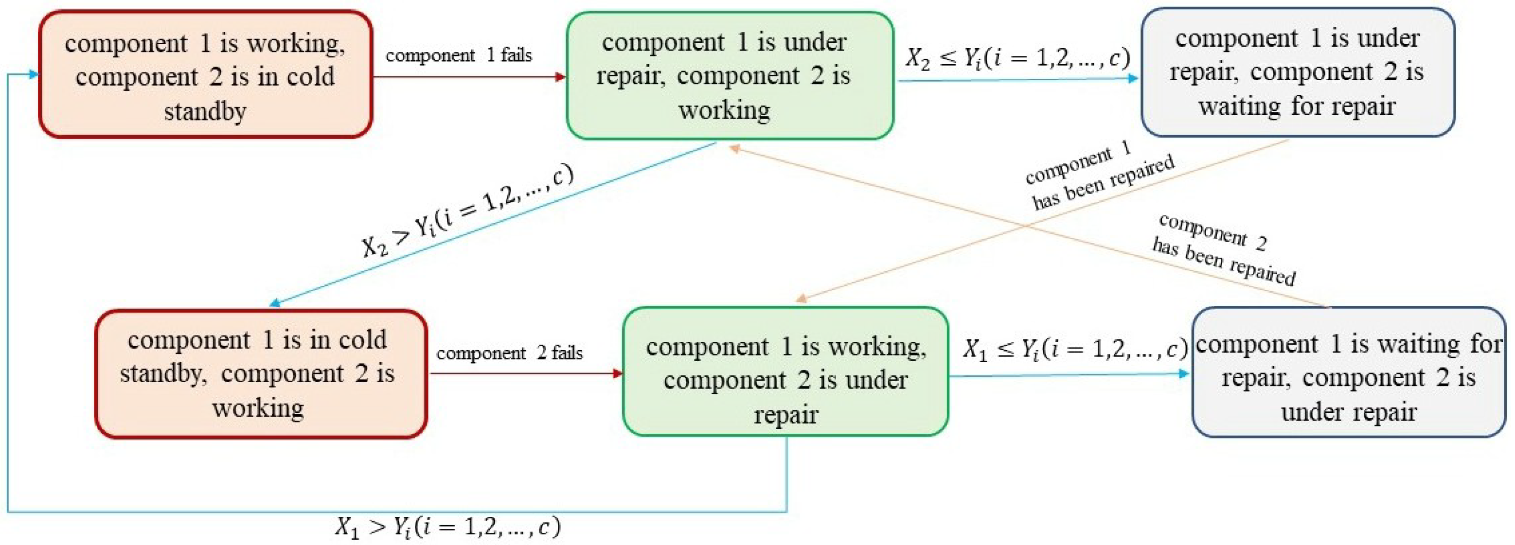
In the following, a repairable cold standby system with two heterogeneous components is considered, which is subject to multiple distinct failure modes. The system is characterized by the following assumptions:

• The system comprises two heterogeneous components. Initially, component 1 is operational, while component 2 remains in a cold standby state. Upon failure of the operating component, the standby component immediately switches to the working state.
• The operating time of component 1, denoted by $X_1$, follows an exponential distribution with failure rate ${\lambda }_1\ge 0$. Its cumulative distribution function is given by $F_1\left(t\right)=P\{X_1\le t\}=1-e^{-{\lambda }_{1}t},t\ge 0$. Similarly, the operating time of component 2, denoted by $X_2$, is exponentially distributed with failure rate ${\lambda }_2\ge 0$, and its cumulative distribution function is $F_2\left(t\right)=P\{X_2\le t\}=1-e^{-{\lambda }_{2}t},t\ge 0$.
• Each component may fail due to any of c mutually independent failure modes. Let $p_i$ denote the probability that a failure of component 1 is of type i, where $p_i\ge 0$ and ${\sum }_{i=1}^c{p}_i=1$, and $q_i$ be the probability that a failure of component 2 is of type j, where $q_j\ge 0$ and ${\sum }_{j=1}^c{q}_j=1$.
• The repair time for a failure of type i, denoted by $Y_i$, follows a general distribution with cumulative distribution function $G_i\left(t\right)=P\{Y_i\le t\},t\ge 0,i=1,2,\dots ,c$. The mean repair time is $\mathbb{E}\left[Y_i\right]={\int }_0^{\infty }td{G}_i\left(t\right)$. The failed component after repaired is as good as new condition.
• All random variables in the system, namely, $X_1$, $X_2$, and $Y_i$ for $i=1,2,\dots ,c$ are mutually independent.

The schematic diagram depicting the architecture of the proposed system is shown in Figure 1.

The following symbols and their descriptions listed in

Table 1. Symbol descriptions in the proposed reliability system.

Symbol	Description
$h\left(s\right)$	The Laplace–Stieltjes transform of an arbitrary function $H\left(t\right)$, defined as $h\left(s\right)={\int }_0^{\infty }{e}^{-st}dH\left(t\right)$.
$h^{\ast }\left(s\right)$	The Laplace transform of $H\left(t\right)$, given by $h^{\ast }\left(s\right)={\int }_0^{\infty }{e}^{-st}H\left(t\right)dt$.
$(H\ast L)\left(t\right)$	The convolution of functions $H\left(t\right)$ and $L\left(t\right)$, expressed as $(H\ast L)\left(t\right)={\int }_0^{\infty }H(t-u)dL\left(u\right)={\int }_0^{\infty }L(t-u)dH\left(u\right)$.
${\Phi }_{\iota }\left(t\right)$	The cumulative distribution function of the time to the first system failure under initial condition $\iota$.
$T_{\iota }$	The mean time to the first system failure under initial condition $\iota$.
$A_{\iota }\left(t\right)$	The system availability at time t under initial condition $\iota$.
$A_{\iota }$	The limiting average system availability under initial condition $\iota$.
$M_{\iota }^{\left(\sigma \right)}\left(t\right)$	The expected number of failures of type $\sigma$ by time t under initial condition $\iota$.
$m_{\iota }^{\left(\sigma \right)}$	The steady-state rate of occurrence of failures of type $\sigma$ under initial condition $\iota$.

will be used throughout the paper.

3. System Analysis

According to the model description, the number of possible failed components in the system is 0, 1, or 2. Additionally, two supplementary variables are introduced to record the types of failure modes occurring in component 1 and component 2, respectively.

(1)

${\vartheta }_1$: The failure mode of component 1, ${\vartheta }_1=1,2,\dots ,c$;

(2)

${\vartheta }_2$: The failure mode of component 2, ${\vartheta }_2=1,2,\dots ,c$.

Furthermore, we discuss the system with the following three cases.

(I)

If the number of failed components in the system is 0, it indicates that both components are normal, with one component in the working state and the other in the cold standby state. Specifically:

• $(0,\underline{0})$: Component 1 is normal and in the working state, while component 2 is in the cold standby state;
• $(\underline{0},0)$: Component 1 is in the cold standby state, while component 2 is normal and in the working state.

(II)

If the number of failed components in the system is 1, it indicates that one of the two components has failed, while the other is in the working state. This is denoted by:

• $({\vartheta }_1,0)$: Component 1 has experienced a ${\vartheta }_1$-type failure mode and is currently under repair, while component 2 is normal and in the working state;
• $(0,{\vartheta }_2)$: Component 1 is normal and in the working state, while component 2 has experienced a ${\vartheta }_2$-type failure mode and is currently under repair.

(III)

If the number of failed components in the system is 2, it indicates that both components have failed, with one currently under repair and the other waiting to be repaired. We set the following:

• $({\vartheta }_1,\overline{{\vartheta }_2})$, ${\vartheta }_1,{\vartheta }_2=1,2,\dots ,c$: Component 1 has experienced a ${\vartheta }_1$-type failure mode and is currently under repair, while component 2 has experienced a ${\vartheta }_2$-type failure mode and is waiting for repair;
• $(\overline{{\vartheta }_1},{\vartheta }_2)$, ${\vartheta }_1,{\vartheta }_2=1,2,\dots ,c$: Component 1 has experienced a ${\vartheta }_1$-type failure mode and is waiting for repair, while component 2 has experienced a ${\vartheta }_2$-type failure mode and is currently under repair.

Thus, the state space of the system is

$$\begin{array}{c}\hfill \Omega =\{(0,\underline{0}),(\underline{0},0),({\vartheta }_1,0),(0,{\vartheta }_2),({\vartheta }_1,\overline{{\vartheta }_2}),(\overline{{\vartheta }_1},{\vartheta }_2),{\vartheta }_1,{\vartheta }_2=1,2,\dots ,c\},\end{array}$$

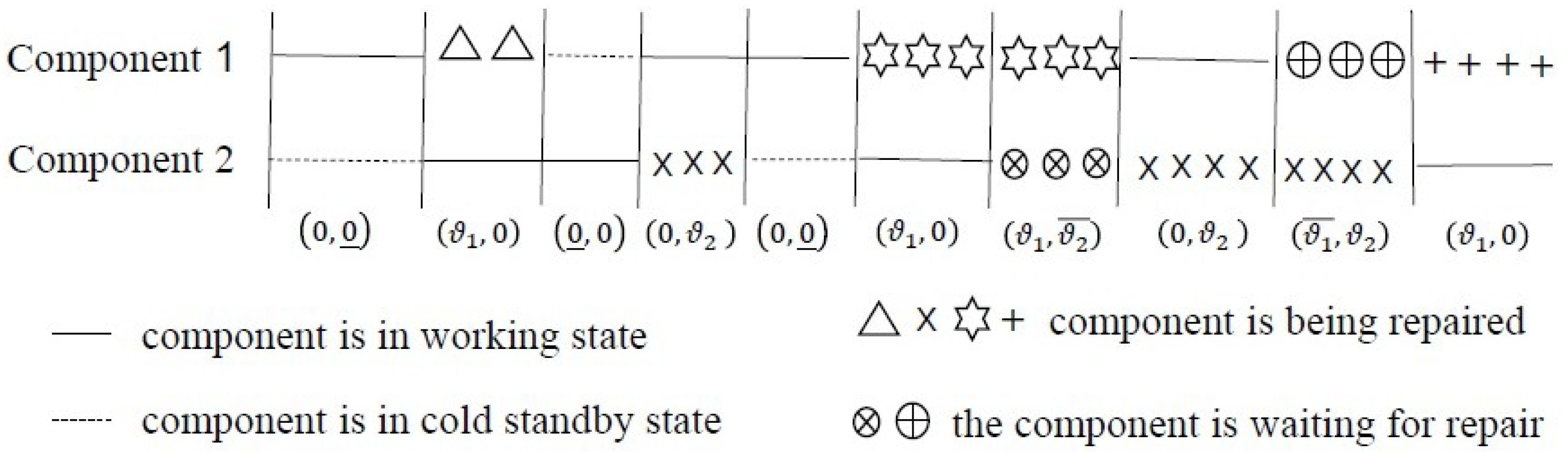
where the working state set is $W=\{(0,\underline{0}),(\underline{0},0),({\vartheta }_1,0),(0,{\vartheta }_2),{\vartheta }_1,{\vartheta }_2=1,2,\dots ,c\}$ and the failure state set is $F=\{({\vartheta }_1,\overline{{\vartheta }_2}),(\overline{{\vartheta }_1},{\vartheta }_2),{\vartheta }_1,{\vartheta }_2=1,2,\dots ,c\}$. The state transition diagram of the reliability model is also given in Figure 2.

Due to the exponential distribution of working time and the general distribution of repair time, the system does not exhibit the Markov property at arbitrary time points, but only at certain special time points. Therefore, the Markov renewal process theory is chosen to analyze this model.

Let ${\tau }_m$ be the time of the m-th system state transition, with ${\tau }_0=0$, and let $Z_m=Z({\tau }_m+0)$ represent the state entered by the system immediately after the m–th transition. According to the model description, $\{(Z_m,{\tau }_m);m=0,1,\dots \}$ is a Markov renewal process on the state space $\Omega$. For $t\ge 0$, the semi–Markov kernel is defined as:

$$Q_{\iota ,\kappa }\left(t\right)=P\{Z_{m+1}=\kappa ,{\tau }_{m+1}-{\tau }_m\le t|Z_m=\iota \},\iota ,\kappa \in \Omega .$$

(1)

Based on the process diagram in Figure 2, there are several scenarios for transitions between system states, including the following eight scenarios.

Scenario 1: $(0,\underline{0})\to ({\vartheta }_1,0)$. This indicates that component 1 has experienced a ${\vartheta }_1$-type failure mode, and component 2 has switched from the cold standby state to the working state. Then

$$\begin{array}{ccc}\hfill Q_{(0,\underline{0}),({\vartheta }_1,0)}\left(t\right)& =& P\{Z_{m+1}=({\vartheta }_1,0),{\tau }_{m+1}-{\tau }_m\le t|Z_m=(0,\underline{0})\}\hfill \\ & =& P\left\{\mathrm{the}\mathrm{working}\mathrm{component}1\mathrm{occurs}\mathrm{the}{\vartheta }_1\mathrm{type}\mathrm{failure}\mathrm{mode}\right\}\hfill \\ & =& p_{{\vartheta }_1}P\{X_1\le t\}=p_{{\vartheta }_1}(1-e^{-{\lambda }_{1}t}).\hfill \end{array}$$

Scenario 2: $(\underline{0},0)\to (0,{\vartheta }_2)$. This indicates that component 2 has experienced a ${\vartheta }_2$-type failure mode, and component 1 has switched from cold standby to working state. Therefore,

$$\begin{array}{ccc}\hfill Q_{(\underline{0},0),(0,{\vartheta }_2)}\left(t\right)& =& P\{Z_{m+1}=(0,{\vartheta }_2),{\tau }_{m+1}-{\tau }_m\le t|Z_m=(\underline{0},0)\}\hfill \\ & =& P\left\{\mathrm{the}\mathrm{working}\mathrm{component}2\mathrm{occurs}\mathrm{the}{\vartheta }_2\mathrm{type}\mathrm{failure}\mathrm{mode}\right\}\hfill \\ & =& q_{{\vartheta }_2}(1-e^{-{\lambda }_{2}t}).\hfill \end{array}$$

Scenario 3: $(0,{\vartheta }_2)\to (0,\underline{0})$. Component 1 remains operational, and component 2 has been repaired and switched to cold standby.

$$\begin{array}{ccc}\hfill Q_{(0,{\vartheta }_2),(0,\underline{0})}\left(t\right)& =& P\{Z_{m+1}=(0,\underline{0}),{\tau }_{m+1}-{\tau }_m\le t|Z_m=(0,{\vartheta }_2)\}\hfill \\ & =& P\{X_1>Y_{{\vartheta }_2},Y_{{\vartheta }_2}\le t\}\hfill \\ & =& {\int }_0^t{e}^{-{\lambda }_{1}u}d{G}_{{\vartheta }_2}\left(u\right).\hfill \end{array}$$

Scenario 4: $({\vartheta }_1,0)\to (\underline{0},0)$. Component 1 has been repaired and switched to cold standby, while component 2 remains operational.

$$\begin{array}{ccc}\hfill Q_{({\vartheta }_1,0),(\underline{0},0)}\left(t\right)& =& P\{Z_{m+1}=(\underline{0},0),{\tau }_{m+1}-{\tau }_m\le t|Z_m=({\vartheta }_1,0)\}\hfill \\ & =& P\{X_2>Y_{{\vartheta }_1},Y_{{\vartheta }_1}\le t\}\hfill \\ & =& {\int }_0^t{e}^{-{\lambda }_{2}u}d{G}_{{\vartheta }_1}\left(u\right).\hfill \end{array}$$

Scenario 5: $(0,{\vartheta }_2)\to (\overline{{\vartheta }_1},{\vartheta }_2)$. Component 1 fails (${\vartheta }_1$-type), while component 2 is still under repair.

$$\begin{array}{ccc}\hfill Q_{(0,{\vartheta }_2),(\overline{{\vartheta }_1},{\vartheta }_2)}\left(t\right)& =& P\{Z_{m+1}=(\overline{{\vartheta }_1},{\vartheta }_2),{\tau }_{m+1}-{\tau }_m\le t|Z_m=(0,{\vartheta }_2)\}\hfill \\ & =& p_{{\vartheta }_1}P\{X_1\le t,Y_{{\vartheta }_2}>X_1\}\hfill \\ & =& p_{{\vartheta }_1}{\int }_0^t\overline{G_{{\vartheta }_2}\left(u\right)}d{F}_1\left(u\right).\hfill \end{array}$$

Scenario 6: $({\vartheta }_1,0)\to ({\vartheta }_1,\overline{{\vartheta }_2})$. Component 2 fails (${\vartheta }_2$-type), while component 1 is under repaired.

$$\begin{array}{ccc}\hfill Q_{({\vartheta }_1,0),({\vartheta }_1,\overline{{\vartheta }_2})}\left(t\right)& =& P\{Z_{m+1}=({\vartheta }_1,\overline{{\vartheta }_2}),{\tau }_{m+1}-{\tau }_m\le t|Z_m=({\vartheta }_1,0)\}\hfill \\ & =& q_{{\vartheta }_2}P\{X_2\le t,Y_{{\vartheta }_1}>X_2\}\hfill \\ & =& q_{{\vartheta }_2}{\int }_0^t\overline{G_{{\vartheta }_1}\left(u\right)}d{F}_2\left(u\right).\hfill \end{array}$$

Since states $({\vartheta }_1,\overline{{\vartheta }_2})$, $(\overline{{\vartheta }_1},{\vartheta }_2)$, ${\vartheta }_1,{\vartheta }_2=1,\dots ,c$ are system failure states, and the entry times into these states are not regeneration points, we define the passing state kernel:

$$Q_{\iota ,\kappa }^v\left(t\right)=P\{Z_{m+1}=\kappa ,{\tau }_{m+1}-{\tau }_m\le t, \mathrm{passing}\mathrm{through}\mathrm{the}\mathrm{state}v|Z_m=\iota \},\iota ,\kappa ,v\in \Omega .$$

(2)

Scenario 7: $({\vartheta }_1,\overline{{\vartheta }_2})\to (0,{\vartheta }_2)$. Because the time of entering the state $({\vartheta }_1,\overline{{\vartheta }_2})$ is not a regeneration point of the system, but a system failure state, we can consider the probability of from state $({\vartheta }_1,0)$ to state $(0,{\vartheta }_2)$ via state $({\vartheta }_1,\overline{{\vartheta }_2})$. Then,

$$\begin{array}{ccc}\hfill Q_{({\vartheta }_1,0),(0,{\vartheta }_2)}^{({\vartheta }_1,\overline{{\vartheta }_2})}\left(t\right)& =& P\{Z_{m+1}=(0,{\vartheta }_2),{\tau }_{m+1}-{\tau }_m\le t, \mathrm{passing}\mathrm{state}({\vartheta }_1,\overline{{\vartheta }_2})|Z_m=({\vartheta }_1,0)\}\hfill \\ & =& q_{{\vartheta }_2}P\{Y_{{\vartheta }_1}\le t,X_2<Y_{{\vartheta }_1}\}\hfill \\ & =& q_{{\vartheta }_2}{\int }_0^t(1-e^{-{\lambda }_{2}u})d{G}_{{\vartheta }_1}\left(u\right).\hfill \end{array}$$

Scenario 8: $(\overline{{\vartheta }_1},{\vartheta }_2)\to ({\vartheta }_1,0)$, via $(\overline{{\vartheta }_1},{\vartheta }_2)$, ${\vartheta }_1,{\vartheta }_2=1,\dots ,c$. Similarly to the analysis in Scenario 7, we get

$$\begin{array}{ccc}\hfill Q_{(0,{\vartheta }_2),({\vartheta }_1,0),}^{(\overline{{\vartheta }_1},{\vartheta }_2)}\left(t\right)& =& P\{Z_{m+1}=({\vartheta }_1,0),{\tau }_{m+1}-{\tau }_m\le t, \mathrm{passing}\mathrm{state}(\overline{{\vartheta }_1},{\vartheta }_2)|Z_m=(0,{\vartheta }_2)\}\hfill \\ & =& p_{{\vartheta }_1}P\{Y_{{\vartheta }_2}\le t,X_1<Y_{{\vartheta }_2}\}\hfill \\ & =& p_{{\vartheta }_1}{\int }_0^t(1-e^{-{\lambda }_{1}u})d{G}_{{\vartheta }_2}\left(u\right).\hfill \end{array}$$

Transforming the semi-Markov kernel via the Laplace–Stieltjes transform gives:

$$\begin{array}{ccc}& & q_{(0,\underline{0}),({\vartheta }_1,0)}\left(s\right)={\displaystyle \frac{p_{{\vartheta }_1}{\lambda }_1}{s+{\lambda }_1}},\hfill \end{array}$$

(3)

$$\begin{array}{ccc}& & q_{(\underline{0},0),(0,{\vartheta }_2)}\left(s\right)={\displaystyle \frac{q_{{\vartheta }_2}{\lambda }_2}{s+{\lambda }_2}},\hfill \end{array}$$

(4)

$$\begin{array}{ccc}& & q_{(0,{\vartheta }_2),(0,\underline{0})}\left(s\right)=g_{{\vartheta }_2}(s+{\lambda }_1),\hfill \end{array}$$

(5)

$$\begin{array}{ccc}& & q_{({\vartheta }_1,0),(\underline{0},0)}\left(s\right)=g_{{\vartheta }_1}(s+{\lambda }_2),\hfill \end{array}$$

(6)

$$\begin{array}{ccc}& & q_{(0,{\vartheta }_2),(\overline{{\vartheta }_1},{\vartheta }_2)}\left(s\right)={\displaystyle \frac{p_{{\vartheta }_1}{\lambda }_1}{s+{\lambda }_1}}\left[1-g_{{\vartheta }_2}(s+{\lambda }_1)\right],\hfill \end{array}$$

(7)

$$\begin{array}{ccc}& & q_{({\vartheta }_1,0),({\vartheta }_1,\overline{{\vartheta }_2})}\left(s\right)={\displaystyle \frac{q_{{\vartheta }_2}{\lambda }_2}{s+{\lambda }_2}}\left[1-g_{{\vartheta }_1}(s+{\lambda }_2)\right],\hfill \end{array}$$

(8)

$$\begin{array}{ccc}& & q_{({\vartheta }_1,0),(0,{\vartheta }_2)}^{({\vartheta }_1,\overline{{\vartheta }_2})}\left(s\right)=q_{{\vartheta }_2}\left[g_{{\vartheta }_1}\left(s\right)-g_{{\vartheta }_1}(s+{\lambda }_2)\right],\hfill \end{array}$$

(9)

$$\begin{array}{ccc}& & q_{(0,{\vartheta }_2),({\vartheta }_1,0)}^{(\overline{{\vartheta }_1},{\vartheta }_2)}\left(s\right)=p_{{\vartheta }_1}\left[g_{{\vartheta }_2}\left(s\right)-g_{{\vartheta }_2}(s+{\lambda }_1)\right],\hfill \end{array}$$

(10)

for ${\vartheta }_j=1,\dots ,c$, $j=1,2$, where $g_{{\vartheta }_j}\left(s\right)$ denotes the Laplace–Stieltjes transform of the repair time distribution $G_{{\vartheta }_j}\left(t\right)$.

4. Reliability Analysis

In this section, we discuss the expressions of the time to the first system failure, the system availability, and the rate of occurrence of system failures.

4.1. The Mean Time to the First System Failure

Firstly, we present the expressions of the distribution function of the first system failure and its mean under initial condition $W=\{(0,\underline{0}),(\underline{0},0),({\vartheta }_1,0),(0,{\vartheta }_2),{\vartheta }_1,{\vartheta }_2=1,2,\dots ,c\}$. Let T represent the time before the first system failure, then

$$\begin{array}{c}\hfill {\Phi }_{\iota }\left(t\right)=P\{T\le t|Z_0=\iota \},T_{\iota }={\int }_0^{\infty }td{\Phi }_{\iota }\left(t\right),\iota \in W.\end{array}$$

Theorem 1.

The Laplace–Stieltjes transform ${\varphi }_{\iota }\left(s\right)={\int }_0^{\infty }{e}^{-st}d{\Phi }_{\iota }\left(t\right)$ of ${\Phi }_{\iota }\left(t\right)$ is

$$\begin{array}{c}\hfill {\varphi }_{(0,\underline{0})}\left(s\right)={\displaystyle \frac{{\left({\displaystyle \frac{{\lambda }_1}{s+{\lambda }_1}}\right)}^2{\displaystyle \frac{{\lambda }_2}{s+{\lambda }_2}}{\sum }_{{\vartheta }_1=1}^c{p}_{{\vartheta }_1}{g}_{{\vartheta }_1}(s+{\lambda }_2){\sum }_{{\vartheta }_2=1}^c{q}_{{\vartheta }_2}[1-g_{{\vartheta }_2}(s+{\lambda }_1)]}{1-{\displaystyle \frac{{\lambda }_1}{s+{\lambda }_1}}{\sum }_{{\vartheta }_1=1}^c{p}_{{\vartheta }_1}{g}_{{\vartheta }_1}(s+{\lambda }_2){\displaystyle \frac{{\lambda }_2}{s+{\lambda }_2}}{\sum }_{{\vartheta }_2=1}^c{q}_{{\vartheta }_2}{g}_{{\vartheta }_2}(s+{\lambda }_1)}}\\ \hfill +{\displaystyle \frac{{\displaystyle \frac{{\lambda }_1}{s+{\lambda }_1}}{\displaystyle \frac{{\lambda }_2}{s+{\lambda }_2}}{\sum }_{{\vartheta }_1=1}^c{p}_{{\vartheta }_1}[1-g_{{\vartheta }_1}(s+{\lambda }_2)]}{1-{\displaystyle \frac{{\lambda }_1}{s+{\lambda }_1}}{\sum }_{{\vartheta }_1=1}^c{p}_{{\vartheta }_1}{g}_{{\vartheta }_1}(s+{\lambda }_2){\displaystyle \frac{{\lambda }_2}{s+{\lambda }_2}}{\sum }_{{\vartheta }_2=1}^c{q}_{{\vartheta }_2}{g}_{{\vartheta }_2}(s+{\lambda }_1)}},\end{array}$$

(11)

$$\begin{array}{c}\hfill {\varphi }_{(\underline{0},0)}\left(s\right)={\displaystyle \frac{{\displaystyle \frac{{\lambda }_1}{s+{\lambda }_1}}{\left({\displaystyle \frac{{\lambda }_2}{s+{\lambda }_2}}\right)}^2{\sum }_{{\vartheta }_2=1}^c{q}_{{\vartheta }_2}{g}_{{\vartheta }_2}(s+{\lambda }_1){\sum }_{{\vartheta }_1=1}^c{p}_{{\vartheta }_1}[1-g_{{\vartheta }_1}(s+{\lambda }_2)]}{1-{\displaystyle \frac{{\lambda }_1}{s+{\lambda }_1}}{\sum }_{{\vartheta }_1=1}^c{p}_{{\vartheta }_1}{g}_{{\vartheta }_1}(s+{\lambda }_2){\displaystyle \frac{{\lambda }_2}{s+{\lambda }_2}}{\sum }_{{\vartheta }_2=1}^c{q}_{{\vartheta }_2}{g}_{{\vartheta }_2}(s+{\lambda }_1)}}\\ \hfill +{\displaystyle \frac{{\displaystyle \frac{{\lambda }_1}{s+{\lambda }_1}}{\displaystyle \frac{{\lambda }_2}{s+{\lambda }_2}}{\sum }_{{\vartheta }_2=1}^c{q}_{{\vartheta }_2}[1-g_{{\vartheta }_2}(s+{\lambda }_1)]}{1-{\displaystyle \frac{{\lambda }_1}{s+{\lambda }_1}}{\sum }_{{\vartheta }_1=1}^c{p}_{{\vartheta }_1}{g}_{{\vartheta }_1}(s+{\lambda }_2){\displaystyle \frac{{\lambda }_2}{s+{\lambda }_2}}{\sum }_{{\vartheta }_2=1}^c{p}_{{\vartheta }_2}{g}_{{\vartheta }_2}(s+{\lambda }_1)}},\end{array}$$

(12)

$$\begin{array}{ccc}& & {\varphi }_{(0,{\vartheta }_2)}\left(s\right)={\varphi }_{(0,\underline{0})}\left(s\right)g_{{\vartheta }_2}(s+{\lambda }_1)+{\displaystyle \frac{{\lambda }_1}{s+{\lambda }_1}}[1-g_{{\vartheta }_2}(s+{\lambda }_1)],\hfill \end{array}$$

(13)

$$\begin{array}{ccc}& & {\varphi }_{({\vartheta }_1,0)}\left(s\right)={\varphi }_{(\underline{0},0)}\left(s\right)g_{{\vartheta }_1}(s+{\lambda }_2)+{\displaystyle \frac{{\lambda }_2}{s+{\lambda }_2}}[1-g_{{\vartheta }_1}(s+{\lambda }_2)],\hfill \end{array}$$

(14)

and the mean time to the first system failure $T_{\iota },\iota \in W$ is obtained as follows,

$$\begin{array}{ccc}& & T_{(0,\underline{0})}={\displaystyle \frac{1}{{\lambda }_1}}+{\displaystyle \frac{{\lambda }_1+{\lambda }_2{\sum }_{{\vartheta }_1=1}^c{p}_{{\vartheta }_1}{g}_{{\vartheta }_1}\left({\lambda }_2\right)}{{\lambda }_1{\lambda }_2[1-{\sum }_{{\vartheta }_1=1}^c{p}_{{\vartheta }_1}{g}_{{\vartheta }_1}\left({\lambda }_2\right){\sum }_{{\vartheta }_2=1}^c{q}_{{\vartheta }_2}{g}_{{\vartheta }_2}\left({\lambda }_1\right)]}},\hfill \end{array}$$

(15)

$$\begin{array}{ccc}& & T_{(\underline{0},0)}={\displaystyle \frac{1}{{\lambda }_2}}+{\displaystyle \frac{{\lambda }_2+{\lambda }_1{\sum }_{{\vartheta }_2=1}^c{q}_{{\vartheta }_2}{g}_{{\vartheta }_2}\left({\lambda }_1\right)}{{\lambda }_1{\lambda }_2[1-{\sum }_{{\vartheta }_1=1}^c{p}_{{\vartheta }_1}{g}_{{\vartheta }_1}\left({\lambda }_2\right){\sum }_{{\vartheta }_2=1}^c{q}_{{\vartheta }_2}{g}_{{\vartheta }_2}\left({\lambda }_1\right)]}},\hfill \end{array}$$

(16)

$$\begin{array}{ccc}& & T_{(0,{\vartheta }_2)}={\displaystyle \frac{1}{{\lambda }_1}}+{\displaystyle \frac{[{\lambda }_1+{\lambda }_2{\sum }_{{\vartheta }_1=1}^c{p}_{{\vartheta }_1}{g}_{{\vartheta }_1}\left({\lambda }_2\right)]g_{{\vartheta }_2}\left({\lambda }_1\right)}{{\lambda }_1{\lambda }_2[1-{\sum }_{{\vartheta }_1=1}^c{p}_{{\vartheta }_1}{g}_{{\vartheta }_1}\left({\lambda }_2\right){\sum }_{{\vartheta }_2=1}^c{q}_{{\vartheta }_2}{g}_{{\vartheta }_2}\left({\lambda }_1\right)]}},\hfill \end{array}$$

(17)

$$\begin{array}{ccc}& & T_{({\vartheta }_1,0)}={\displaystyle \frac{1}{{\lambda }_2}}+{\displaystyle \frac{[{\lambda }_2+{\lambda }_1{\sum }_{{\vartheta }_2=1}^c{q}_{{\vartheta }_2}{g}_{{\vartheta }_2}\left({\lambda }_1\right)]g_{{\vartheta }_1}\left({\lambda }_2\right)}{{\lambda }_1{\lambda }_2[1-{\sum }_{{\vartheta }_1=1}^c{p}_{{\vartheta }_1}{g}_{{\vartheta }_1}\left({\lambda }_2\right){\sum }_{{\vartheta }_2=1}^c{q}_{{\vartheta }_2}{g}_{{\vartheta }_2}\left({\lambda }_1\right)]}}.\hfill \end{array}$$

(18)

for ${\vartheta }_j=1,\dots ,c$, $j=1,2$.

Proof. 

When $\iota =(0,\underline{0})$, both components are normal, that is, component 1 is in working state, while component 2 is in cold standby state. Then, it can be obtained that

$$\begin{array}{ccc}\hfill {\Phi }_{(0,\underline{0})}\left(t\right)& =& P\{T\le t|Z_0=(0,\underline{0})\}\hfill \\ & =& \sum _{{\vartheta }_1=1}^c{\int }_0^{t}P\{T\le t-u|Z_1=({\vartheta }_1,0)\}dP\{Z_1=({\vartheta }_1,0),{\tau }_1-{\tau }_0\le u|Z_0=(0,\underline{0})\}\hfill \\ & =& \sum _{{\vartheta }_1=1}^c{\int }_0^t{\Phi }_{({\vartheta }_1,0)}(t-u)d{Q}_{(0,\underline{0}),({\vartheta }_1,0)}\left(u\right)\hfill \\ & =& \sum _{{\vartheta }_1=1}^c{\Phi }_{({\vartheta }_1,0)}\left(t\right)\ast Q_{(0,\underline{0}),({\vartheta }_1,0)}\left(t\right).\hfill \end{array}$$

With $\iota =(\underline{0},0)$, where component 1 is in cold standby and component 2 is in the working state, both components are normal. Then, we have

$$\begin{array}{ccc}\hfill {\Phi }_{(\underline{0},0)}\left(t\right)& =& P\{T\le t|Z_0=(\underline{0},0)\}\hfill \\ & =& \sum _{{\vartheta }_2=1}^c{\int }_0^{t}P\{T\le t-u|Z_1=(0,{\vartheta }_2)\}dP\{Z_1=(0,{\vartheta }_2),{\tau }_1-{\tau }_0\le u|Z_0=(\underline{0},0)\}\hfill \\ & =& \sum _{{\vartheta }_2=1}^c{\int }_0^t{\Phi }_{(0,{\vartheta }_2)}(t-u)d{Q}_{(\underline{0},0),(0,{\vartheta }_2)}\left(u\right)\hfill \\ & =& \sum _{{\vartheta }_2=1}^c{\Phi }_{(0,{\vartheta }_2)}\left(t\right)\ast Q_{(\underline{0},0),(0,{\vartheta }_2)}\left(t\right).\hfill \end{array}$$

It is noted that, for $\iota =(0,{\vartheta }_2)$, component 1 functions normally, while component 2 suffers a ${\vartheta }_2$-type failure, and is currently being repaired. Accordingly, we get

$$\begin{array}{ccc}\hfill {\Phi }_{(0,{\vartheta }_2)}\left(t\right)& =& P\{T\le t|Z_0=(0,{\vartheta }_2)\}\hfill \\ & =& {\int }_0^{t}P\{T\le t-u|Z_1=(0,\underline{0})\}dP\{Z_1=(0,\underline{0}),{\tau }_1-{\tau }_0\le u|Z_0=(0,{\vartheta }_2)\}\hfill \\ & +& \sum _{{\vartheta }_1=1}^{c}P\{Z_1=(\overline{{\vartheta }_1},{\vartheta }_2),T\le t|Z_0=(0,{\vartheta }_2)\}\hfill \\ & =& {\int }_0^t{\Phi }_{(0,\underline{0})}(t-u)d{Q}_{(0,{\vartheta }_2),(0,\underline{0})}\left(u\right)+\sum _{{\vartheta }_1=1}^c{Q}_{(0,{\vartheta }_2),(\overline{{\vartheta }_1},{\vartheta }_2)}\left(t\right)\hfill \\ & =& {\Phi }_{(0,\underline{0})}\left(t\right)\ast Q_{(0,{\vartheta }_2),(0,\underline{0})}\left(t\right)+\sum _{{\vartheta }_1=1}^c{Q}_{(0,{\vartheta }_2),(\overline{{\vartheta }_1},{\vartheta }_2)}\left(t\right).\hfill \end{array}$$

If $\iota =({\vartheta }_1,0)$, then component 1 has undergone a ${\vartheta }_1$ failure and is under repair, whereas component 2 remains normal and operational. This concludes that

$$\begin{array}{ccc}\hfill {\Phi }_{({\vartheta }_1,0)}\left(t\right)& =& P\{T\le t|Z_0=({\vartheta }_1,0)\}\hfill \\ & =& {\int }_0^{t}P\{T\le t-u|Z_1=(\underline{0},0)\}dP\{Z_1=(\underline{0},0),{\tau }_1-{\tau }_0\le u|Z_0=({\vartheta }_1,0)\}\hfill \\ & +& \sum _{{\vartheta }_2=1}^{c}P\{Z_1=({\vartheta }_1,\overline{{\vartheta }_2}),T\le t|Z_0=({\vartheta }_1,0)\}\hfill \\ & =& {\int }_0^t{\Phi }_{(\underline{0},0)}(t-u)d{Q}_{({\vartheta }_1,0),(\underline{0},0)}\left(u\right)+\sum _{{\vartheta }_2=1}^c{Q}_{({\vartheta }_1,0),({\vartheta }_1,\overline{{\vartheta }_2})}\left(t\right)\hfill \\ & =& {\Phi }_{(\underline{0},0)}\left(t\right)\ast Q_{({\vartheta }_1,0),(\underline{0},0)}\left(t\right)+\sum _{{\vartheta }_2=1}^c{Q}_{({\vartheta }_1,0),({\vartheta }_1,\overline{{\vartheta }_2})}\left(t\right).\hfill \end{array}$$

Application of the Laplace–Stieltjes transform on ${\Phi }_{\iota }\left(t\right),\iota \in W$ yields

$$\begin{array}{ccc}& & {\varphi }_{(0,\underline{0})}\left(s\right)=\sum _{{\vartheta }_1=1}^c{\varphi }_{({\vartheta }_1,0)}\left(s\right)q_{(0,\underline{0}),({\vartheta }_1,0)}\left(s\right),\hfill \\ & & {\varphi }_{(\underline{0},0)}\left(s\right)=\sum _{{\vartheta }_2=1}^c{\varphi }_{(0,{\vartheta }_2)}\left(s\right)q_{(\underline{0},0),(0,{\vartheta }_2)}\left(s\right),\hfill \\ & & {\varphi }_{(0,{\vartheta }_2)}\left(s\right)={\varphi }_{(0,\underline{0})}\left(s\right)q_{(0,{\vartheta }_2),(0,\underline{0})}\left(s\right)+\sum _{{\vartheta }_1=1}^c{q}_{(0,{\vartheta }_2),(\overline{{\vartheta }_1},{\vartheta }_2)}\left(s\right),\hfill \\ & & {\varphi }_{({\vartheta }_1,0)}\left(s\right)={\varphi }_{(\underline{0},0)}\left(s\right)q_{({\vartheta }_1,0),(\underline{0},0)}\left(s\right)+\sum _{{\vartheta }_2=1}^c{q}_{({\vartheta }_1,0),({\vartheta }_1,\overline{{\vartheta }_2})}\left(s\right).\hfill \end{array}$$

Substituting the values of $q_{\iota ,\kappa }\left(s\right)$ in (3)–(10) into ${\varphi }_{\iota ,\kappa }\left(s\right)$, respectively, we have

$$\begin{array}{ccc}& & {\varphi }_{(0,\underline{0})}\left(s\right)={\displaystyle \frac{{\lambda }_1}{s+{\lambda }_1}}\sum _{{\vartheta }_1=1}^c{p}_{{\vartheta }_1}{\varphi }_{({\vartheta }_1,0)}\left(s\right),\hfill \\ & & {\varphi }_{(\underline{0},0)}\left(s\right)={\displaystyle \frac{{\lambda }_2}{s+{\lambda }_2}}\sum _{{\vartheta }_2=1}^c{q}_{{\vartheta }_2}{\varphi }_{(0,{\vartheta }_2)}\left(s\right),\hfill \\ & & {\varphi }_{(0,{\vartheta }_2)}\left(s\right)={\varphi }_{(0,\underline{0})}\left(s\right)g_{{\vartheta }_2}(s+{\lambda }_1)+{\displaystyle \frac{{\lambda }_1}{s+{\lambda }_1}}[1-g_{{\vartheta }_2}(s+{\lambda }_1)],\hfill \\ & & {\varphi }_{({\vartheta }_1,0)}\left(s\right)={\varphi }_{(\underline{0},0)}\left(s\right)g_{{\vartheta }_1}(s+{\lambda }_2)+{\displaystyle \frac{{\lambda }_2}{s+{\lambda }_2}}[1-g_{{\vartheta }_1}(s+{\lambda }_2)].\hfill \end{array}$$

The values of ${\varphi }_{\iota ,\kappa }\left(s\right)$ can be directly obtained by solving these equations simultaneously. Furthermore, the mean time to the first system failure is derived by $T_{\iota }=-d{\varphi }_{\iota }{\left(s\right)/ds|}_{s=0}$ and we omit the detail. This completes the proof. □

4.2. The System Availability

For $t\ge 0$, let

$$\begin{array}{c}\hfill A_{\iota }=P\left\{\mathrm{the}\mathrm{system}\mathrm{is}\mathrm{operating}\mathrm{at}\mathrm{time}t\right|Z_0=\iota \},\iota \in W.\end{array}$$

Theorem 2.

The Laplace transform $a_{\iota }^{\ast }\left(s\right)={\int }_0^{\infty }{e}^{-st}{A}_{\iota }\left(t\right)dt$ of system availability is

$$\begin{array}{c}\hfill a_{(0,\underline{0})}^{\ast }\left(s\right)={\displaystyle \frac{{\displaystyle \frac{1}{s+{\lambda }_1}}+{\displaystyle \frac{{\lambda }_1}{s+{\lambda }_1}}{\sum }_{{\vartheta }_1=1}^c{p}_{{\vartheta }_1}{\eta }_{{\vartheta }_1,0}\left(s\right)+{\displaystyle \frac{1}{s+{\lambda }_2}}{\displaystyle \frac{{\lambda }_1}{s+{\lambda }_1}}{\sum }_{{\vartheta }_1=1}^c{p}_{{\vartheta }_1}{\xi }_{{\vartheta }_1,0}\left(s\right)}{1-{\displaystyle \frac{{\lambda }_1}{s+{\lambda }_1}}{\sum }_{{\vartheta }_1=1}^c{p}_{{\vartheta }_1}{\xi }_{{\vartheta }_1,0}\left(s\right){\displaystyle \frac{{\lambda }_2}{s+{\lambda }_2}}{\sum }_{{\vartheta }_2=1}^c{q}_{{\vartheta }_2}{\xi }_{0,{\vartheta }_2}\left(s\right)}}\\ \hfill +{\displaystyle \frac{{\displaystyle \frac{{\lambda }_1}{s+{\lambda }_1}}{\sum }_{{\vartheta }_1=1}^c{p}_{{\vartheta }_1}{\xi }_{{\vartheta }_1,0}\left(s\right){\displaystyle \frac{{\lambda }_2}{s+{\lambda }_2}}{\sum }_{{\vartheta }_2=1}^c{q}_{{\vartheta }_2}{\eta }_{0,{\vartheta }_2}\left(s\right)}{1-{\displaystyle \frac{{\lambda }_1}{s+{\lambda }_1}}{\sum }_{{\vartheta }_1=1}^c{p}_{{\vartheta }_1}{\xi }_{{\vartheta }_1,0}\left(s\right){\displaystyle \frac{{\lambda }_2}{s+{\lambda }_2}}{\sum }_{{\vartheta }_2=1}^c{q}_{{\vartheta }_2}{\xi }_{0,{\vartheta }_2}\left(s\right)}},\end{array}$$

(19)

$$\begin{array}{c}\hfill a_{(\underline{0},0)}^{\ast }\left(s\right)={\displaystyle \frac{{\displaystyle \frac{1}{s+{\lambda }_2}}+{\displaystyle \frac{{\lambda }_2}{s+{\lambda }_2}}{\sum }_{{\vartheta }_2=1}^c{q}_{{\vartheta }_2}{\eta }_{0,{\vartheta }_2}\left(s\right)+{\displaystyle \frac{1}{s+{\lambda }_1}}{\displaystyle \frac{{\lambda }_2}{s+{\lambda }_2}}{\sum }_{{\vartheta }_2=1}^c{q}_{{\vartheta }_2}{\xi }_{0,{\vartheta }_2}\left(s\right)}{1-{\displaystyle \frac{{\lambda }_1}{s+{\lambda }_1}}{\sum }_{{\vartheta }_1=1}^c{p}_{{\vartheta }_1}{\xi }_{{\vartheta }_1,0}\left(s\right){\displaystyle \frac{{\lambda }_2}{s+{\lambda }_2}}{\sum }_{{\vartheta }_2=1}^c{q}_{{\vartheta }_2}{\xi }_{0,{\vartheta }_2}\left(s\right)}}\\ \hfill +{\displaystyle \frac{{\displaystyle \frac{{\lambda }_1}{s+{\lambda }_1}}{\sum }_{{\vartheta }_1=1}^c{p}_{{\vartheta }_1}{\eta }_{{\vartheta }_1,0}\left(s\right){\displaystyle \frac{{\lambda }_2}{s+{\lambda }_2}}{\sum }_{{\vartheta }_2=1}^c{q}_{{\vartheta }_2}{\xi }_{0,{\vartheta }_2}\left(s\right)}{1-{\displaystyle \frac{{\lambda }_1}{s+{\lambda }_1}}{\sum }_{{\vartheta }_1=1}^c{p}_{{\vartheta }_1}{\xi }_{{\vartheta }_1,0}\left(s\right){\displaystyle \frac{{\lambda }_2}{s+{\lambda }_2}}{\sum }_{{\vartheta }_2=1}^c{q}_{{\vartheta }_2}{\xi }_{0,{\vartheta }_2}\left(s\right)}},\end{array}$$

(20)

$$\begin{array}{c}\hfill a_{(0,{\vartheta }_2)}^{\ast }\left(s\right)={\xi }_{0,{\vartheta }_2}\left(s\right)a_{(0,\underline{0})}^{\ast }\left(s\right)+{\eta }_{0,{\vartheta }_2}\left(s\right),\end{array}$$

(21)

$$\begin{array}{c}\hfill a_{({\vartheta }_1,0)}^{\ast }\left(s\right)={\xi }_{{\vartheta }_1,0}\left(s\right)a_{(\underline{0},0)}^{\ast }\left(s\right)+{\eta }_{{\vartheta }_1,0}\left(s\right),\end{array}$$

(22)

for ${\vartheta }_j=1,\dots ,c$, $j=1,2$, where

$$\begin{array}{ccc}& & {\xi }_{0,{\vartheta }_2}\left(s\right)={\displaystyle \frac{s[g_{{\vartheta }_2}\left(s\right)-g_{{\vartheta }_2}(s+{\lambda }_1)]+{\lambda }_1{g}_{{\vartheta }_2}\left(s\right)}{{\lambda }_1}},\hfill \\ & & {\eta }_{0,{\vartheta }_2}\left(s\right)={\displaystyle \frac{1-g_{{\vartheta }_2}(s+{\lambda }_1)}{s+{\lambda }_1}}-{\displaystyle \frac{g_{{\vartheta }_2}\left(s\right)-g_{{\vartheta }_2}(s+{\lambda }_1)}{{\lambda }_1}},\hfill \\ & & {\xi }_{{\vartheta }_1,0}\left(s\right)={\displaystyle \frac{s[g_{{\vartheta }_1}\left(s\right)-g_{{\vartheta }_1}(s+{\lambda }_2)]+{\lambda }_2{g}_{{\vartheta }_1}\left(s\right)}{{\lambda }_2}},\hfill \\ & & {\eta }_{{\vartheta }_1,0}\left(s\right)={\displaystyle \frac{1-g_{{\vartheta }_1}(s+{\lambda }_2)}{s+{\lambda }_2}}-{\displaystyle \frac{g_{{\vartheta }_1}\left(s\right)-g_{{\vartheta }_1}(s+{\lambda }_2)}{{\lambda }_2}},\hfill \end{array}$$

and the limiting average system availability $A_{\iota }={lim}_{t\to \infty }{\displaystyle \frac{1}{t}}{\int }_0^t{A}_{\iota }\left(s\right)ds$ is

$$\begin{array}{c}\hfill A=A_{\iota }={\displaystyle \frac{{\lambda }_1+{\lambda }_2}{\begin{array}{c}\{{\lambda }_1{\sum }_{{\vartheta }_1=1}^c{p}_{{\vartheta }_1}{g}_{{\vartheta }_1}\left({\lambda }_2\right)+{\lambda }_2{\sum }_{{\vartheta }_2=1}^c{q}_{{\vartheta }_2}{g}_{{\vartheta }_2}\left({\lambda }_1\right)\\ +{\lambda }_1{\lambda }_2{\sum }_{{\vartheta }_1=1}^c{p}_{{\vartheta }_1}E\left[Y_{{\vartheta }_1}\right]+{\lambda }_1{\lambda }_2{\sum }_{{\vartheta }_2=1}^c{q}_{{\vartheta }_2}E\left[Y_{{\vartheta }_2}\right]\}\end{array}}}\end{array}$$

(23)

Proof. 

Similar to the proof of Theorem 1, we still discuss the availability of the system in four cases. If $\iota =(0,\underline{0})$, it follows from the states of two components that

$$\begin{array}{ccc}\hfill A_{(0,\underline{0})}\left(t\right)& =& P\left\{\mathrm{the}\mathrm{system}\mathrm{is}\mathrm{operating}\mathrm{at}\mathrm{time}t\right|Z_0=(0,\underline{0})\}\hfill \\ & =& P\{X_1>t\}\hfill \\ & +& \sum _{{\vartheta }_1=1}^c{\int }_0^{t}P\{\mathrm{the}\mathrm{system}\mathrm{is}\mathrm{operating}\mathrm{at}\mathrm{time}t-u|Z_1=({\vartheta }_1,0)\}d{Q}_{(0,\underline{0}),({\vartheta }_1,0)}\left(u\right)\hfill \\ & =& e^{-{\lambda }_{1}t}+\sum _{{\vartheta }_1=1}^c{\int }_0^t{A}_{({\vartheta }_1,0)}(t-u)d{Q}_{(0,\underline{0}),({\vartheta }_1,0)}\left(u\right)\hfill \\ & =& e^{-{\lambda }_{1}t}+\sum _{{\vartheta }_1=1}^c{A}_{({\vartheta }_1,0)}\left(t\right)\ast Q_{(0,\underline{0}),({\vartheta }_1,0)}\left(t\right)\hfill \end{array}$$

As for the case of $\iota =(\underline{0},0)$, we derive

$$\begin{array}{ccc}\hfill A_{(\underline{0},0)}\left(t\right)& =& P\left\{\mathrm{the}\mathrm{system}\mathrm{is}\mathrm{operating}\mathrm{at}\mathrm{time}t\right|Z_0=(\underline{0},0)\}\hfill \\ & =& P\{X_2>t\}\hfill \\ & +& \sum _{{\vartheta }_2=1}^c{\int }_0^{t}P\{\mathrm{the}\mathrm{system}\mathrm{is}\mathrm{operating}\mathrm{at}\mathrm{time}t-u|Z_1=(0,{\vartheta }_2)\}d{Q}_{(\underline{0},0),(0,{\vartheta }_2)}\left(u\right)\hfill \\ & =& e^{-{\lambda }_{2}t}+\sum _{{\vartheta }_2=1}^c{\int }_0^t{A}_{(0,{\vartheta }_2)}(t-u)d{Q}_{(\underline{0},0),(0,{\vartheta }_2)}\left(u\right)\hfill \\ & =& e^{-{\lambda }_{2}t}+\sum _{{\vartheta }_2=1}^c{A}_{(0,{\vartheta }_2)}\left(t\right)\ast Q_{(\underline{0},0),(0,{\vartheta }_2)}\left(t\right)\hfill \end{array}$$

Then, considering the third case, namely, $\iota =(0,{\vartheta }_2)$, one can get

$$\begin{array}{ccc}\hfill A_{(0,{\vartheta }_2)}\left(t\right)& =& P\left\{\mathrm{the}\mathrm{system}\mathrm{is}\mathrm{operating}\mathrm{at}\mathrm{time}t\right|Z_0=(0,{\vartheta }_2)\}\hfill \\ & =& P\{X_1>t,Y_{{\vartheta }_2}>t\}\hfill \\ & +& P\{\mathrm{the}\mathrm{system}\mathrm{is}\mathrm{operating}\mathrm{at}\mathrm{time}t,Z_1=(0,\underline{0})|Z_0=(0,{\vartheta }_2)\}\hfill \\ & +& \sum _{{\vartheta }_1=1}^c{\int }_0^{t}P\{\mathrm{the}\mathrm{system}\mathrm{is}\mathrm{operating}\mathrm{at}\mathrm{time}t-u|Z_1=({\vartheta }_1,0)\}d{Q}_{(0,{\vartheta }_2),({\vartheta }_1,0)}^{(\overline{{\vartheta }_1},{\vartheta }_2)}\left(u\right)\hfill \\ & =& e^{-{\lambda }_{1}t}[1-G_{{\vartheta }_2}\left(t\right)]+{\int }_0^t{A}_{(0,\underline{0})}(t-u)d{Q}_{(0,{\vartheta }_2),(0,\underline{0})}\left(u\right)\hfill \\ & +& \sum _{{\vartheta }_1=1}^c{\int }_0^t{A}_{({\vartheta }_1,0)}(t-u)d{Q}_{(0,{\vartheta }_2),({\vartheta }_1,0)}^{(\overline{{\vartheta }_1},{\vartheta }_2)}\left(u\right)\hfill \\ & =& e^{-{\lambda }_{1}t}[1-G_{{\vartheta }_2}\left(t\right)]+A_{(0,\underline{0})}\left(t\right)\ast Q_{(0,{\vartheta }_2),(0,\underline{0})}\left(t\right)+\sum _{{\vartheta }_1=1}^c{A}_{({\vartheta }_1,0)}\left(t\right)\ast Q_{(0,{\vartheta }_2),({\vartheta }_1,0)}^{(\overline{{\vartheta }_1},{\vartheta }_2)}\left(t\right).\hfill \end{array}$$

For the last case, when $\iota =({\vartheta }_1,0)$, it concludes that

$$\begin{array}{ccc}\hfill A_{({\vartheta }_1,0)}\left(t\right)& =& P\left\{\mathrm{the}\mathrm{system}\mathrm{is}\mathrm{operating}\mathrm{at}\mathrm{time}t\right|Z_0=({\vartheta }_1,0)\}\hfill \\ & =& P\{X_2>t,Y_{{\vartheta }_1}>t\}\hfill \\ & +& P\{\mathrm{the}\mathrm{system}\mathrm{is}\mathrm{operating}\mathrm{at}\mathrm{time}t,Z_1=(\underline{0},0)|Z_0=({\vartheta }_1,0)\}\hfill \\ & +& \sum _{{\vartheta }_2=1}^c{\int }_0^{t}P\{\mathrm{the}\mathrm{system}\mathrm{is}\mathrm{operating}\mathrm{at}\mathrm{time}t-u|Z_1=(0,{\vartheta }_2)\}d{Q}_{({\vartheta }_1,0),(0,{\vartheta }_2)}^{({\vartheta }_1,\overline{{\vartheta }_2})}\left(u\right)\hfill \\ & =& e^{-{\lambda }_{2}t}[1-G_{{\vartheta }_1}\left(t\right)]+{\int }_0^t{A}_{(\underline{0},0)}(t-u)d{Q}_{({\vartheta }_1,0),(\underline{0},0)}\left(u\right)\hfill \\ & +& \sum _{{\vartheta }_2=1}^c{\int }_0^t{A}_{(0,{\vartheta }_2)}(t-u)d{Q}_{({\vartheta }_1,0),(0,{\vartheta }_2)}^{({\vartheta }_1,\overline{{\vartheta }_2})}\left(u\right)\hfill \\ & =& e^{-{\lambda }_{2}t}[1-G_{{\vartheta }_1}\left(t\right)]+A_{(\underline{0},0)}\left(t\right)\ast Q_{({\vartheta }_1,0),(\underline{0},0)}\left(t\right)+\sum _{{\vartheta }_2=1}^c{A}_{(0,{\vartheta }_2)}\left(t\right)\ast Q_{({\vartheta }_1,0),(0,{\vartheta }_2)}^{({\vartheta }_1,\overline{{\vartheta }_2})}\left(t\right)\hfill \end{array}$$

Next, we take the Laplace transform for above four results, respectively, and obtain

$$\begin{array}{ccc}& & a_{(0,\underline{0})}^{\ast }\left(s\right)={\displaystyle \frac{1}{s+{\lambda }_1}}+\sum _{{\vartheta }_1=1}^c{a}_{({\vartheta }_1,0)}^{\ast }\left(s\right)q_{(0,\underline{0}),({\vartheta }_1,0)}\left(s\right),\hfill \\ & & a_{(\underline{0},0)}^{\ast }\left(s\right)={\displaystyle \frac{1}{s+{\lambda }_2}}+\sum _{{\vartheta }_2=1}^c{a}_{(0,{\vartheta }_2)}^{\ast }\left(s\right)q_{(\underline{0},0),(0,{\vartheta }_2)}\left(s\right),\hfill \\ & & a_{(0,{\vartheta }_2)}^{\ast }\left(s\right)={\displaystyle \frac{1}{s+{\lambda }_1}}[1-g_{{\vartheta }_2}(s+{\lambda }_1)]+a_{(0,\underline{0})}^{\ast }\left(s\right)q_{(0,{\vartheta }_2),(0,\underline{0})}\left(s\right)+\sum _{{\vartheta }_1=1}^c{a}_{({\vartheta }_1,0)}^{\ast }\left(s\right)q_{(0,{\vartheta }_2),({\vartheta }_1,0)}^{(\overline{{\vartheta }_1},{\vartheta }_2)}\left(s\right),\hfill \\ & & a_{({\vartheta }_1,0)}^{\ast }\left(s\right)={\displaystyle \frac{1}{s+{\lambda }_2}}[1-g_{{\vartheta }_1}(s+{\lambda }_2)]+a_{(\underline{0},0)}^{\ast }\left(s\right)q_{({\vartheta }_1,0),(\underline{0},0)}\left(s\right)+\sum _{{\vartheta }_2=1}^c{a}_{(0,{\vartheta }_2)}^{\ast }\left(s\right)q_{({\vartheta }_1,0),(0,{\vartheta }_2)}^{({\vartheta }_1,\overline{{\vartheta }_2})}\left(s\right)\hfill \end{array}$$

Substituting $q_{\iota ,\kappa }\left(s\right)$ in (3)–(10) into $a_{\iota ,\kappa }^{\ast }\left(s\right)$, respectively, one can get

$$\begin{array}{ccc}& & a_{(0,\underline{0})}^{\ast }\left(s\right)={\displaystyle \frac{1}{s+{\lambda }_1}}+{\displaystyle \frac{{\lambda }_1}{s+{\lambda }_1}}\sum _{{\vartheta }_1=1}^c{p}_{{\vartheta }_1}{a}_{({\vartheta }_1,0)}^{\ast }\left(s\right),\hfill \\ & & a_{(\underline{0},0)}^{\ast }\left(s\right)={\displaystyle \frac{1}{s+{\lambda }_2}}+{\displaystyle \frac{{\lambda }_2}{s+{\lambda }_2}}\sum _{{\vartheta }_2=1}^c{q}_{{\vartheta }_2}{a}_{(0,{\vartheta }_2)}^{\ast }\left(s\right),\hfill \\ & & a_{(0,{\vartheta }_2)}^{\ast }\left(s\right)={\displaystyle \frac{1}{s+{\lambda }_1}}[1-g_{{\vartheta }_2}(s+{\lambda }_1)]+a_{(0,\underline{0})}^{\ast }\left(s\right)g_{{\vartheta }_2}(s+{\lambda }_1)\hfill \\ & & +\sum _{{\vartheta }_1=1}^c{a}_{({\vartheta }_1,0)}^{\ast }\left(s\right)p_{{\vartheta }_1}[g_{{\vartheta }_2}\left(s\right)-g_{{\vartheta }_2}(s+{\lambda }_1)],\hfill \\ & & a_{({\vartheta }_1,0)}^{\ast }\left(s\right)={\displaystyle \frac{1}{s+{\lambda }_2}}[1-g_{{\vartheta }_1}(s+{\lambda }_2)]+a_{(\underline{0},0)}^{\ast }\left(s\right)g_{{\vartheta }_1}(s+{\lambda }_2)\hfill \\ & & +\sum _{{\vartheta }_2=1}^c{a}_{(0,{\vartheta }_2)}^{\ast }\left(s\right)q_{{\vartheta }_2}[g_{{\vartheta }_1}\left(s\right)-g_{{\vartheta }_1}(s+{\lambda }_2)].\hfill \end{array}$$

The values of $a_{\iota ,\kappa }^{\ast }\left(s\right)$ can be directly obtained by solving these equations simultaneously. Note that

$$\begin{array}{ccc}& & {\xi }_{{\vartheta }_1,0}\left(0\right)=1,{\eta }_{{\vartheta }_1,0}\left(0\right)=0,{\xi }_{0,{\vartheta }_2}\left(0\right)=1,{\eta }_{0,{\vartheta }_2}\left(0\right)=0,\hfill \end{array}$$

(24)

$$\begin{array}{ccc}& & {\displaystyle \frac{d{\xi }_{{\vartheta }_1,0}\left(s\right)}{ds}}{|}_{s=0}={\displaystyle \frac{1-g_{{\vartheta }_1}\left({\lambda }_2\right)-{\lambda }_{2}E\left[Y_{{\vartheta }_1}\right]}{{\lambda }_2}},\hfill \end{array}$$

(25)

$$\begin{array}{ccc}& & {\displaystyle \frac{d{\xi }_{0,{\vartheta }_2}\left(s\right)}{ds}}{|}_{s=0}={\displaystyle \frac{1-g_{{\vartheta }_2}\left({\lambda }_1\right)-{\lambda }_{1}E\left[Y_{{\vartheta }_2}\right]}{{\lambda }_1}}.\hfill \end{array}$$

(26)

Thus, the limitation of the average system availability $A_{\iota }={lim}_{t\to \infty }{\displaystyle \frac{1}{t}}{\int }_0^t{A}_{\iota }\left(s\right)ds={lim}_{s\to 0^{+}}s{a}_{\iota }^{\ast }\left(s\right)$ can be derived. □

4.3. The Rate of Occurrence of System Failures

For $t\ge 0$, let $N^{\left({\sigma }_1\right)}\left(t\right),({\sigma }_1=1,2,\cdots ,c)$ be the number of system failures in $(0,t]$ caused by the ${\sigma }_1$-type failure mode of component 1, $N^{\left({\sigma }_2\right)}\left(t\right),({\sigma }_2=1,2,\cdots ,c)$ be the number of system failures in $(0,t]$ caused by the ${\sigma }_2$-type failure mode of component 2, and $N\left(t\right)$ be the number of system failures in $(0,t]$. Furthermore, let

$$\begin{array}{c}\hfill M_{\iota }^{\left({\sigma }_1\right)}\left(t\right)=E\left[N^{\left({\sigma }_1\right)}\left(t\right)\right|Z_0=\iota ],M_{\iota }^{\left({\sigma }_2\right)}\left(t\right)=E\left[N^{\left({\sigma }_2\right)}\left(t\right)\right|Z_0=\iota ],\\ \hfill M^{\left(\sigma \right)}\left(t\right)=E\left[N\left(t\right)\right|Z_0=\iota ],\iota \in W,{\sigma }_1,{\sigma }_2=1,2,\cdots ,c.\end{array}$$

Theorem 3.

The Laplace–Stieltjes transform $m_{\iota }^{\left({\sigma }_1\right)}\left(s\right)$ and $m_{\iota }^{\left({\sigma }_2\right)}\left(s\right)$ is

$$\begin{array}{ccc}& & m_{(0,\underline{0})}^{\left({\sigma }_1\right)}\left(s\right)={\displaystyle \frac{p_{{\sigma }_1}{\left({\displaystyle \frac{{\lambda }_1}{s+{\lambda }_1}}\right)}^2{\displaystyle \frac{{\lambda }_2}{s+{\lambda }_2}}{\sum }_{{\vartheta }_1=1}^c{p}_{{\vartheta }_1}{\xi }_{{\vartheta }_1,0}\left(s\right){\sum }_{{\vartheta }_2=1}^c{q}_{{\vartheta }_2}[1-g_{{\vartheta }_2}(s+{\lambda }_1)]}{1-{\displaystyle \frac{{\lambda }_1}{s+{\lambda }_1}}{\sum }_{{\vartheta }_1=1}^c{p}_{{\vartheta }_1}{\xi }_{{\vartheta }_1,0}\left(s\right){\displaystyle \frac{{\lambda }_2}{s+{\lambda }_2}}{\sum }_{{\vartheta }_2=1}^c{q}_{{\vartheta }_2}{\xi }_{0,{\vartheta }_2}\left(s\right)}},\hfill \end{array}$$

(27)

$$\begin{array}{ccc}& & m_{(\underline{0},0)}^{\left({\sigma }_1\right)}\left(s\right)={\displaystyle \frac{p_{{\sigma }_1}{\displaystyle \frac{{\lambda }_1}{s+{\lambda }_1}}{\displaystyle \frac{{\lambda }_2}{s+{\lambda }_2}}{\sum }_{{\vartheta }_2=1}^c{q}_{{\vartheta }_2}[1-g_{{\vartheta }_2}(s+{\lambda }_1)]}{1-{\displaystyle \frac{{\lambda }_1}{s+{\lambda }_1}}{\sum }_{{\vartheta }_1=1}^c{p}_{{\vartheta }_1}{\xi }_{{\vartheta }_1,0}\left(s\right){\displaystyle \frac{{\lambda }_2}{s+{\lambda }_2}}{\sum }_{{\vartheta }_2=1}^c{q}_{{\vartheta }_2}{\xi }_{0,{\vartheta }_2}\left(s\right)}},\hfill \end{array}$$

(28)

$$\begin{array}{ccc}& & m_{(0,{\vartheta }_2)}^{\left({\sigma }_1\right)}\left(s\right)={\xi }_{0,{\vartheta }_2}\left(s\right)m_{(0,\underline{0})}^{\left({\sigma }_1\right)}\left(s\right)+p_{{\sigma }_1}{\displaystyle \frac{{\lambda }_1}{s+{\lambda }_1}}[1-g_{{\vartheta }_2}(s+{\lambda }_1)],\hfill \end{array}$$

(29)

$$\begin{array}{ccc}& & m_{({\vartheta }_1,0)}^{\left({\sigma }_1\right)}\left(s\right)={\xi }_{{\vartheta }_1,0}\left(s\right)m_{(\underline{0},0)}^{\left({\sigma }_1\right)}\left(s\right),\hfill \end{array}$$

(30)

$$\begin{array}{ccc}& & m_{(0,\underline{0})}^{\left({\sigma }_2\right)}\left(s\right)={\displaystyle \frac{q_{{\sigma }_2}{\displaystyle \frac{{\lambda }_1}{s+{\lambda }_1}}{\displaystyle \frac{{\lambda }_2}{s+{\lambda }_2}}{\sum }_{{\vartheta }_1=1}^c{p}_{{\vartheta }_1}[1-g_{{\vartheta }_1}(s+{\lambda }_2)]}{1-{\displaystyle \frac{{\lambda }_1}{s+{\lambda }_1}}{\sum }_{{\vartheta }_1=1}^c{p}_{{\vartheta }_1}{\xi }_{{\vartheta }_1,0}\left(s\right){\displaystyle \frac{{\lambda }_2}{s+{\lambda }_2}}{\sum }_{{\vartheta }_2=1}^c{q}_{{\vartheta }_2}{\xi }_{0,{\vartheta }_2}\left(s\right)}},\hfill \end{array}$$

(31)

$$\begin{array}{ccc}& & m_{(\underline{0},0)}^{\left({\sigma }_2\right)}\left(s\right)={\displaystyle \frac{q_{{\sigma }_2}{\displaystyle \frac{{\lambda }_1}{s+{\lambda }_1}}{\left({\displaystyle \frac{{\lambda }_2}{s+{\lambda }_2}}\right)}^2{\sum }_{{\vartheta }_2=1}^c{q}_{{\vartheta }_2}{\xi }_{0,{\vartheta }_2}\left(s\right){\sum }_{{\vartheta }_1=1}^c{p}_{{\vartheta }_1}[1-g_{{\vartheta }_1}(s+{\lambda }_2)]}{1-{\displaystyle \frac{{\lambda }_1}{s+{\lambda }_1}}{\sum }_{{\vartheta }_1=1}^c{p}_{{\vartheta }_1}{\xi }_{{\vartheta }_1,0}\left(s\right){\displaystyle \frac{{\lambda }_2}{s+{\lambda }_2}}{\sum }_{{\vartheta }_2=1}^c{q}_{{\vartheta }_2}{\xi }_{0,{\vartheta }_2}\left(s\right)}},\hfill \end{array}$$

(32)

$$\begin{array}{ccc}& & m_{(0,{\vartheta }_2)}^{\left({\sigma }_2\right)}\left(s\right)={\xi }_{0,{\vartheta }_2}\left(s\right)m_{(0,\underline{0})}^{\left({\sigma }_2\right)}\left(s\right)\hfill \end{array}$$

(33)

$$\begin{array}{ccc}& & m_{({\vartheta }_1,0)}^{\left({\sigma }_2\right)}\left(s\right)={\xi }_{{\vartheta }_1,0}\left(s\right)m_{(\underline{0},0)}^{\left({\sigma }_2\right)}\left(s\right)+q_{{\sigma }_2}{\displaystyle \frac{{\lambda }_2}{s+{\lambda }_2}}[1-g_{{\vartheta }_1}(s+{\lambda }_2)],\hfill \end{array}$$

(34)

and the rate of occurrence of system failures caused by the ${\sigma }_1$ and ${\sigma }_2$-type failure mode is

$$\begin{array}{ccc}& & m^{\left({\sigma }_1\right)}={\displaystyle \frac{p_{{\sigma }_1}{\lambda }_1{\lambda }_2{\sum }_{{\vartheta }_2=1}^c{q}_{{\vartheta }_2}[1-g_{{\vartheta }_2}\left({\lambda }_1\right)]}{\begin{array}{c}\{{\lambda }_1{\sum }_{{\vartheta }_1=1}^c{p}_{{\vartheta }_1}{g}_{{\vartheta }_1}\left({\lambda }_2\right)+{\lambda }_2{\sum }_{{\vartheta }_2=1}^c{q}_{{\vartheta }_2}{g}_{{\vartheta }_2}\left({\lambda }_1\right)\\ +{\lambda }_1{\lambda }_2{\sum }_{{\vartheta }_1=1}^c{p}_{{\vartheta }_1}E\left[Y_{{\vartheta }_1}\right]+{\lambda }_1{\lambda }_2{\sum }_{{\vartheta }_2=1}^c{q}_{{\vartheta }_2}E\left[Y_{{\vartheta }_2}\right]\}\end{array}}},\hfill \end{array}$$

(35)

$$\begin{array}{ccc}& & m^{\left({\sigma }_2\right)}={\displaystyle \frac{q_{{\sigma }_2}{\lambda }_1{\lambda }_2{\sum }_{{\vartheta }_1=1}^c{p}_{{\vartheta }_1}[1-g_{{\vartheta }_1}\left({\lambda }_2\right)]}{\begin{array}{c}\{{\lambda }_1{\sum }_{{\vartheta }_1=1}^c{p}_{{\vartheta }_1}{g}_{{\vartheta }_1}\left({\lambda }_2\right)+{\lambda }_2{\sum }_{{\vartheta }_2=1}^c{q}_{{\vartheta }_2}{g}_{{\vartheta }_2}\left({\lambda }_1\right)\\ +{\lambda }_1{\lambda }_2{\sum }_{{\vartheta }_1=1}^c{p}_{{\vartheta }_1}E\left[Y_{{\vartheta }_1}\right]+{\lambda }_1{\lambda }_2{\sum }_{{\vartheta }_2=1}^c{q}_{{\vartheta }_2}E\left[Y_{{\vartheta }_2}\right]\}\end{array}}}\hfill \end{array}$$

(36)

Consequently, the rate of occurrence of system failure is

$$\begin{array}{c}\hfill m={\displaystyle \frac{{\lambda }_1{\lambda }_2[2-{\sum }_{{\vartheta }_1=1}^c{p}_{{\vartheta }_1}{g}_{{\vartheta }_1}\left({\lambda }_2\right)-{\sum }_{{\vartheta }_2=1}^c{q}_{{\vartheta }_2}{g}_{{\vartheta }_2}\left({\lambda }_1\right)]}{\begin{array}{c}\{{\lambda }_1{\sum }_{{\vartheta }_1=1}^c{p}_{{\vartheta }_1}{g}_{{\vartheta }_1}\left({\lambda }_2\right)+{\lambda }_2{\sum }_{{\vartheta }_2=1}^c{q}_{{\vartheta }_2}{g}_{{\vartheta }_2}\left({\lambda }_1\right)\\ +{\lambda }_1{\lambda }_2{\sum }_{{\vartheta }_1=1}^c{p}_{{\vartheta }_1}E\left[Y_{{\vartheta }_1}\right]+{\lambda }_1{\lambda }_2{\sum }_{{\vartheta }_2=1}^c{q}_{{\vartheta }_2}E\left[Y_{{\vartheta }_2}\right]\}\end{array}}}.\end{array}$$

(37)

Proof. 

Similar to the proof method of the previous theorem, we also discuss each failure mode in four cases. The state of each component is no longer presented in detail.

• When $\iota =(0,\underline{0})$, we have

  $$\begin{array}{ccc}\hfill M_{(0,\underline{0})}^{\left({\sigma }_1\right)}\left(t\right)& =& E\left[N^{\left({\sigma }_1\right)}\left(t\right)\right|Z_0=(0,\underline{0})]\hfill \\ & =& \sum _{{\vartheta }_1=1}^c{\int }_0^{t}E\left[N^{\left({\sigma }_1\right)}(t-u)\right|Z_1=({\vartheta }_1,0)]dP\{Z_1=({\vartheta }_1,0),{\tau }_1-{\tau }_0\le u|Z_0=(0,\underline{0})\}\hfill \\ & =& \sum _{{\vartheta }_1=1}^c{\int }_0^t{M}_{({\vartheta }_1,0)}^{\left({\sigma }_1\right)}(t-u)d{Q}_{(0,\underline{0}),({\vartheta }_1,0)}\left(u\right)\hfill \\ & =& \sum _{{\vartheta }_1=1}^c{M}_{({\vartheta }_1,0)}^{\left({\sigma }_1\right)}\left(t\right)\ast Q_{(0,\underline{0}),({\vartheta }_1,0)}\left(t\right),\hfill \end{array}$$

  and

  $$\begin{array}{c}\hfill M_{(0,\underline{0})}^{\left({\sigma }_2\right)}\left(t\right)=E\left[N^{\left({\sigma }_2\right)}\left(t\right)\right|Z_0=(0,\underline{0})]=\sum _{{\vartheta }_1=1}^c{M}_{({\vartheta }_1,0)}^{\left({\sigma }_2\right)}\left(t\right)\ast Q_{(0,\underline{0}),({\vartheta }_1,0)}\left(t\right).\end{array}$$
• When $\iota =(\underline{0},0)$, one has

  $$\begin{array}{ccc}\hfill M_{(\underline{0},0)}^{\left({\sigma }_1\right)}\left(t\right)& =& E\left[N^{\left({\sigma }_1\right)}\left(t\right)\right|Z_0=(\underline{0},0)]\hfill \\ & =& \sum _{{\vartheta }_2=1}^c{\int }_0^{t}E\left[N^{\left({\sigma }_1\right)}(t-u)\right|Z_1=(0,{\vartheta }_2)]dP\{Z_1=(0,{\vartheta }_2),{\tau }_1-{\tau }_0\le u|Z_0=(\underline{0},0)\}\hfill \\ & =& \sum _{{\vartheta }_2=1}^c{\int }_0^t{M}_{(0,{\vartheta }_2)}^{\left({\sigma }_1\right)}(t-u)d{Q}_{(\underline{0},0),(0,{\vartheta }_2)}\left(u\right)\hfill \\ & =& \sum _{{\vartheta }_2=1}^c{M}_{(0,{\vartheta }_2)}^{\left({\sigma }_1\right)}\left(t\right)\ast Q_{(\underline{0},0),(0,{\vartheta }_2)}\left(t\right),\hfill \end{array}$$

  and

  $$\begin{array}{c}\hfill M_{(\underline{0},0)}^{\left({\sigma }_2\right)}\left(t\right)=E\left[N^{\left({\sigma }_2\right)}\left(t\right)\right|Z_0=(\underline{0},0)]=\sum _{{\vartheta }_2=1}^c{M}_{(0,{\vartheta }_2)}^{\left({\sigma }_2\right)}\left(t\right)\ast Q_{(\underline{0},0),(0,{\vartheta }_2)}\left(t\right).\end{array}$$
• For $\iota =(0,{\vartheta }_2)$, we get

  $$\begin{array}{ccc}\hfill M_{(0,{\vartheta }_2)}^{\left({\sigma }_1\right)}\left(t\right)& =& E\left[N^{\left({\sigma }_1\right)}\left(t\right)\right|Z_0=(0,{\vartheta }_2)]\hfill \\ & =& {\int }_0^{t}E\left[N^{\left({\sigma }_1\right)}(t-u)\right|Z_1=(0,\underline{0})]d{Q}_{(0,{\vartheta }_2),(0,\underline{0})}\left(u\right)\hfill \\ & +& \sum _{{\vartheta }_1=1}^c{\int }_0^{t}E\left[N^{\left({\sigma }_1\right)}(t-u)\right|Z_1=({\vartheta }_1,0)]d{Q}_{(0,{\vartheta }_2),({\vartheta }_1,0)}^{(\overline{{\vartheta }_1},{\vartheta }_2)}\left(u\right)\hfill \\ & +& P\{X_1\le t,Y_{{\vartheta }_2}>X_1,\mathrm{in}\mathrm{component}1,\mathrm{the}{\sigma }_1\mathrm{type}\mathrm{failure}\mathrm{mode}\mathrm{occurs}\}\hfill \\ & =& M_{(0,\underline{0})}^{\left({\sigma }_1\right)}\left(t\right)\ast Q_{(0,{\vartheta }_2),(0,\underline{0})}\left(t\right)+\sum _{{\vartheta }_1=1}^c{M}_{({\vartheta }_1,0)}^{\left({\sigma }_1\right)}\left(t\right)\ast Q_{(0,{\vartheta }_2),({\vartheta }_1,0)}^{(\overline{{\vartheta }_1},{\vartheta }_2)}\left(t\right)\hfill \\ & +& Q_{(0,{\vartheta }_2),(\overline{{\sigma }_1},{\vartheta }_2)}\left(t\right),\hfill \end{array}$$

  and

  $$\begin{array}{ccc}\hfill M_{(0,{\vartheta }_2)}^{\left({\sigma }_2\right)}\left(t\right)& =& E\left[N^{\left({\sigma }_2\right)}\left(t\right)\right|Z_0=(0,{\vartheta }_2)]\hfill \\ & =& M_{(0,\underline{0})}^{\left({\sigma }_2\right)}\left(t\right)\ast Q_{(0,{\vartheta }_2),(0,\underline{0})}\left(t\right)+\sum _{{\vartheta }_1=1}^c{M}_{({\vartheta }_1,0)}^{\left({\sigma }_2\right)}\left(t\right)\ast Q_{(0,{\vartheta }_2),({\vartheta }_1,0)}^{(\overline{{\vartheta }_1},{\vartheta }_2)}\left(t\right).\hfill \end{array}$$
• For $\iota =({\vartheta }_1,0)$, we have

  $$\begin{array}{ccc}\hfill M_{({\vartheta }_1,0)}^{\left({\sigma }_1\right)}\left(t\right)& =& E\left[N^{\left({\sigma }_1\right)}\left(t\right)\right|Z_0=({\vartheta }_1,0)]\hfill \\ & =& {\int }_0^{t}E\left[N^{\left({\sigma }_1\right)}(t-u)\right|Z_1=(\underline{0},0)]d{Q}_{({\vartheta }_1,0),(\underline{0},0)}\left(u\right)\hfill \\ & +& \sum _{{\vartheta }_2=1}^c{\int }_0^{t}E\left[N^{\left({\sigma }_1\right)}(t-u)\right|Z_1=(0,{\vartheta }_2)]d{Q}_{({\vartheta }_1,0),(0,{\vartheta }_2)}^{({\vartheta }_1,\overline{{\vartheta }_2})}\left(u\right)\hfill \\ & =& M_{(\underline{0},0)}^{\left({\sigma }_1\right)}\left(t\right)\ast Q_{({\vartheta }_1,0),(\underline{0},0)}\left(t\right)+\sum _{{\vartheta }_2=1}^c{M}_{(0,{\vartheta }_2)}^{\left({\sigma }_1\right)}\left(t\right)\ast Q_{({\vartheta }_1,0),(0,{\vartheta }_2)}^{({\vartheta }_1,\overline{{\vartheta }_2})}\left(t\right),\hfill \end{array}$$

  and

  $$\begin{array}{ccc}\hfill M_{({\vartheta }_1,0)}^{\left({\sigma }_2\right)}\left(t\right)& =& E\left[N^{\left({\sigma }_2\right)}\left(t\right)\right|Z_0=({\vartheta }_1,0)]\hfill \\ & =& {\int }_0^{t}E\left[N^{\left({\sigma }_2\right)}(t-u)\right|Z_1=(\underline{0},0)]d{Q}_{({\vartheta }_1,0),(\underline{0},0)}\left(u\right)\hfill \\ & +& \sum _{{\vartheta }_2=1}^c{\int }_0^{t}E\left[N^{\left({\sigma }_2\right)}(t-u)\right|Z_1=(0,{\vartheta }_2)]d{Q}_{({\vartheta }_1,0),(0,{\vartheta }_2)}^{({\vartheta }_1,\overline{{\vartheta }_2})}\left(u\right)\hfill \\ & +& P\{X_2\le t,Y_{{\vartheta }_1}>X_2,\mathrm{the}\mathrm{component}2\mathrm{failure}\mathrm{mode}{\sigma }_2\mathrm{type}\mathrm{failure}\mathrm{mode}\}\hfill \\ & =& M_{(\underline{0},0)}^{\left({\sigma }_2\right)}\left(t\right)\ast Q_{({\vartheta }_1,0),(\underline{0},0)}\left(t\right)+\sum _{{\vartheta }_2=1}^c{M}_{(0,{\vartheta }_2)}^{\left({\sigma }_2\right)}\left(t\right)\ast Q_{({\vartheta }_1,0),(0,{\vartheta }_2)}^{({\vartheta }_1,\overline{{\vartheta }_2})}\left(t\right)\hfill \\ \hfill & +& Q_{({\vartheta }_1,0),({\vartheta }_1,\overline{{\sigma }_2})}\left(t\right).\hfill \end{array}$$

Taking the Laplace–Stieltjes transform on $M_{\iota }^{\left({\sigma }_1\right)}\left(t\right)$ and $M_{\iota }^{\left({\sigma }_2\right)}\left(t\right)$, $\iota \in W$, we obtain

$$\begin{array}{cc}\hfill & m_{(0,\underline{0})}^{\left({\sigma }_1\right)}\left(s\right)=\sum _{{\vartheta }_1=1}^c{m}_{({\vartheta }_1,0)}^{\left({\sigma }_1\right)}\left(s\right)q_{(0,\underline{0}),({\vartheta }_1,0)}\left(s\right),\hfill \\ \hfill & m_{(0,\underline{0})}^{\left({\sigma }_2\right)}\left(s\right)=\sum _{{\vartheta }_1=1}^c{m}_{({\vartheta }_1,0)}^{\left({\sigma }_2\right)}\left(s\right)q_{(0,\underline{0}),({\vartheta }_1,0)}\left(s\right),\hfill \\ \hfill & m_{(\underline{0},0)}^{\left({\sigma }_1\right)}\left(s\right)=\sum _{{\vartheta }_2=1}^c{m}_{(0,{\vartheta }_2)}^{\left({\sigma }_1\right)}\left(s\right)q_{(\underline{0},0),(0,{\vartheta }_2)}\left(s\right),\hfill \\ \hfill & m_{(\underline{0},0)}^{\left({\sigma }_2\right)}\left(s\right)=\sum _{{\vartheta }_2=1}^c{m}_{(0,{\vartheta }_2)}^{\left({\sigma }_2\right)}\left(s\right)q_{(\underline{0},0),(0,{\vartheta }_2)}\left(s\right),\hfill \\ \hfill & m_{(0,{\vartheta }_2)}^{\left({\sigma }_1\right)}\left(s\right)=m_{(0,\underline{0})}^{\left({\sigma }_1\right)}\left(s\right)q_{(0,{\vartheta }_2),(0,\underline{0})}\left(s\right)+\sum _{{\vartheta }_1=1}^c{m}_{({\vartheta }_1,0)}^{\left({\sigma }_1\right)}\left(s\right)q_{(0,{\vartheta }_2),({\vartheta }_1,0)}^{(\overline{{\vartheta }_1},{\vartheta }_2)}\left(s\right)+q_{(0,{\vartheta }_2),(\overline{{\sigma }_1},{\vartheta }_2)}\left(s\right),\hfill \\ \hfill & m_{(0,{\vartheta }_2)}^{\left({\sigma }_2\right)}\left(s\right)=m_{(0,\underline{0})}^{\left({\sigma }_2\right)}\left(s\right)q_{(0,{\vartheta }_2),(0,\underline{0})}\left(s\right)+\sum _{{\vartheta }_1=1}^c{m}_{({\vartheta }_1,0)}^{\left({\sigma }_2\right)}\left(s\right)q_{(0,{\vartheta }_2),({\vartheta }_1,0)}^{(\overline{{\vartheta }_1},{\vartheta }_2)}\left(s\right),\hfill \\ \hfill & m_{({\vartheta }_1,0)}^{\left({\sigma }_1\right)}\left(s\right)=m_{(\underline{0},0)}^{\left({\sigma }_1\right)}\left(s\right)q_{({\vartheta }_1,0),(\underline{0},0)}\left(s\right)+\sum _{{\vartheta }_2=1}^c{m}_{(0,{\vartheta }_2)}^{\left({\sigma }_1\right)}\left(s\right)q_{({\vartheta }_1,0),(0,{\vartheta }_2)}^{({\vartheta }_1,\overline{{\vartheta }_2})}\left(s\right),\hfill \\ \hfill & m_{({\vartheta }_1,0)}^{\left({\sigma }_2\right)}\left(s\right)=m_{(\underline{0},0)}^{\left({\sigma }_2\right)}\left(s\right)q_{({\vartheta }_1,0),(\underline{0},0)}\left(s\right)+\sum _{{\vartheta }_2=1}^c{m}_{(0,{\vartheta }_2)}^{\left({\sigma }_2\right)}\left(s\right)q_{({\vartheta }_1,0),(0,{\vartheta }_2)}^{({\vartheta }_1,\overline{{\vartheta }_2})}\left(s\right)+q_{({\vartheta }_1,0),({\vartheta }_1,\overline{{\sigma }_2})}\left(s\right).\hfill \end{array}$$

Substituting the values of $q_{\iota ,\kappa }\left(s\right)$ in (3)–(10) into $m_{\iota }^{\left({\sigma }_1\right)}\left(s\right)$ and $m_{\iota }^{\left({\sigma }_2\right)}\left(s\right)$, we have

$$\begin{array}{ccc}& & m_{(0,\underline{0})}^{\left({\sigma }_1\right)}\left(s\right)={\displaystyle \frac{{\lambda }_1}{s+{\lambda }_1}}\sum _{{\vartheta }_1=1}^c{p}_{{\vartheta }_1}{m}_{({\vartheta }_1,0)}^{\left({\sigma }_1\right)}\left(s\right),\hfill \\ & & m_{(0,\underline{0})}^{\left({\sigma }_2\right)}\left(s\right)={\displaystyle \frac{{\lambda }_1}{s+{\lambda }_1}}\sum _{{\vartheta }_1=1}^c{p}_{{\vartheta }_1}{m}_{({\vartheta }_1,0)}^{\left({\sigma }_2\right)}\left(s\right),\hfill \\ & & m_{(\underline{0},0)}^{\left({\sigma }_1\right)}\left(s\right)={\displaystyle \frac{{\lambda }_2}{s+{\lambda }_2}}\sum _{{\vartheta }_2=1}^c{q}_{{\vartheta }_2}{m}_{(0,{\vartheta }_2)}^{\left({\sigma }_1\right)}\left(s\right),\hfill \\ & & m_{(\underline{0},0)}^{\left({\sigma }_2\right)}\left(s\right)={\displaystyle \frac{{\lambda }_2}{s+{\lambda }_2}}\sum _{{\vartheta }_2=1}^c{q}_{{\vartheta }_2}{m}_{(0,{\vartheta }_2)}^{\left({\sigma }_2\right)}\left(s\right),\hfill \\ & & m_{(0,{\vartheta }_2)}^{\left({\sigma }_1\right)}\left(s\right)=m_{(0,\underline{0})}^{\left({\sigma }_1\right)}\left(s\right)g_{{\vartheta }_2}(s+{\lambda }_1)+\sum _{{\vartheta }_1=1}^c{m}_{({\vartheta }_1,0)}^{\left({\sigma }_1\right)}\left(s\right)p_{{\vartheta }_1}[g_{{\vartheta }_2}\left(s\right)-g_{{\vartheta }_2}(s+{\lambda }_1)]\hfill \\ & & +p_{{\sigma }_1}{\displaystyle \frac{{\lambda }_1}{s+{\lambda }_1}}[1-g_{{\vartheta }_2}(s+{\lambda }_1)],\hfill \\ & & m_{(0,{\vartheta }_2)}^{\left({\sigma }_2\right)}\left(s\right)=m_{(0,\underline{0})}^{\left({\sigma }_2\right)}\left(s\right)g_{{\vartheta }_2}(s+{\lambda }_1)+\sum _{{\vartheta }_1=1}^c{m}_{({\vartheta }_1,0)}^{\left({\sigma }_2\right)}\left(s\right)p_{{\vartheta }_1}[g_{{\vartheta }_2}\left(s\right)-g_{{\vartheta }_2}(s+{\lambda }_1)],\hfill \\ & & m_{({\vartheta }_1,0)}^{\left({\sigma }_1\right)}\left(s\right)=m_{(\underline{0},0)}^{\left({\sigma }_1\right)}\left(s\right)g_{{\vartheta }_1}(s+{\lambda }_2)+\sum _{{\vartheta }_2=1}^c{m}_{(0,{\vartheta }_2)}^{\left({\sigma }_1\right)}\left(s\right)q_{{\vartheta }_2}[g_{{\vartheta }_1}\left(s\right)-g_{{\vartheta }_1}(s+{\lambda }_2)],\hfill \\ & & m_{({\vartheta }_1,0)}^{\left({\sigma }_2\right)}\left(s\right)=m_{(\underline{0},0)}^{\left({\sigma }_2\right)}\left(s\right)g_{{\vartheta }_1}(s+{\lambda }_2)+\sum _{{\vartheta }_2=1}^c{m}_{(0,{\vartheta }_2)}^{\left({\sigma }_2\right)}\left(s\right)q_{{\vartheta }_2}[g_{{\vartheta }_1}\left(s\right)-g_{{\vartheta }_1}(s+{\lambda }_2)]\hfill \\ & & +q_{{\sigma }_2}{\displaystyle \frac{{\lambda }_2}{s+{\lambda }_2}}[1-g_{{\vartheta }_1}(s+{\lambda }_2)].\hfill \end{array}$$

The values of $m_{\iota }^{\left({\sigma }_1\right)}\left(s\right)$ and $m_{\iota }^{\left({\sigma }_2\right)}\left(s\right)$ can be directly obtained by solving these equations simultaneously. Furthermore, from (27)–(34), the limitation of the average system availability $m^{\left({\sigma }_{\nu }\right)}={lim}_{t\to \infty }{\displaystyle \frac{1}{t}}{M}_{\iota }^{\left({\sigma }_{\nu }\right)}\left(t\right)={lim}_{s\to 0^{+}}s{m}_{\iota }^{\left({\sigma }_{\nu }\right)}\left(s\right),\nu =1,2$ can be derived, and $m={\sum }_{{\sigma }_1=1}^c{m}^{\left({\sigma }_1\right)}+{\sum }_{{\sigma }_2=1}^c{m}^{\left({\sigma }_2\right)}$. This completes the proof. □

5. Special Cases

We have previously considered a special case in [30] and therefore only provide the corresponding expressions for reliability indicators here.

When ${\lambda }_1={\lambda }_2=\lambda$, $p_i=q_i,i=1,2,\dots ,c$, the analyzed system degrades to a two identical components cold standby repairable system, and the expressions for system reliability indicators are as follows.

(1)

The mean time to the first system failure:

$$\begin{array}{ccc}& & {\varphi }_{(0,\underline{0})}\left(s\right)={\varphi }_{(\underline{0},0)}\left(s\right)={({\displaystyle \frac{\lambda }{s+\lambda }})}^2{\displaystyle \frac{{\sum }_{{\vartheta }_1=1}^c{p}_{{\vartheta }_1}[1-g_{{\vartheta }_1}(s+\lambda )]}{1-{\displaystyle \frac{\lambda }{s+\lambda }}{\sum }_{{\vartheta }_1=1}^c{p}_{{\vartheta }_1}{g}_{{\vartheta }_1}(s+\lambda )}},\hfill \\ & & {\varphi }_{(0,{\vartheta }_2)}\left(s\right)={\varphi }_{({\vartheta }_1,0)}\left(s\right)={\varphi }_{(0,\underline{0})}\left(s\right)g_{{\vartheta }_1}(s+\lambda )+{\displaystyle \frac{\lambda }{s+\lambda }}[1-g_{{\vartheta }_1}(s+\lambda )],\hfill \\ & & T_{(0,\underline{0})}\left(s\right)=T_{(\underline{0},0)}\left(s\right)={\displaystyle \frac{1}{\lambda }}+{\displaystyle \frac{1}{\lambda [1-{\sum }_{{\vartheta }_1=1}^c{p}_{{\vartheta }_1}{g}_{{\vartheta }_1}\left(\lambda \right)]}},\hfill \\ & & T_{(0,{\vartheta }_2)}\left(s\right)=T_{({\vartheta }_1,0)}\left(s\right)={\displaystyle \frac{1}{\lambda }}+{\displaystyle \frac{g_{{\vartheta }_1}\left(\lambda \right)}{\lambda [1-{\sum }_{{\vartheta }_1=1}^c{p}_{{\vartheta }_1}{g}_{{\vartheta }_1}\left(\lambda \right)]}}.\hfill \end{array}$$

(2)

The system availability:

$$\begin{array}{ccc}& & a_{(0,\underline{0})}^{\ast }\left(s\right)=a_{(\underline{0},0)}^{\ast }\left(s\right)={\displaystyle \frac{1}{s+\lambda }}{\displaystyle \frac{1+\lambda {\sum }_{{\vartheta }_1=1}^c{p}_{{\vartheta }_1}{\eta }_{{\vartheta }_1,0}\left(s\right)}{1-{\displaystyle \frac{\lambda }{s+\lambda }}{\sum }_{{\vartheta }_1=1}^c{p}_{{\vartheta }_1}{\xi }_{{\vartheta }_1,0}\left(s\right)}},\hfill \\ & & a_{(0,{\vartheta }_2)}^{\ast }\left(s\right)=a_{({\vartheta }_1,0)}^{\ast }\left(s\right)={\xi }_{{\vartheta }_1,0}\left(s\right)a_{(0,\underline{0})}^{\ast }\left(s\right)+{\eta }_{{\vartheta }_1,0}\left(s\right),\hfill \\ & & A={\displaystyle \frac{1}{{\sum }_{{\vartheta }_1=1}^c{p}_{{\vartheta }_1}{g}_{{\vartheta }_1}\left(\lambda \right)+\lambda {\sum }_{{\vartheta }_1=1}^c{p}_{{\vartheta }_1}E\left[Y_{{\vartheta }_1}\right]}}.\hfill \end{array}$$

where

$$\begin{array}{ccc}& & {\xi }_{{\vartheta }_1,0}\left(s\right)={\xi }_{0,{\vartheta }_2}\left(s\right)={\displaystyle \frac{s[g_{{\vartheta }_1}\left(s\right)-g_{{\vartheta }_1}(s+\lambda )]+\lambda g_{{\vartheta }_1}\left(s\right)}{\lambda }},\hfill \\ & & {\eta }_{{\vartheta }_1,0}\left(s\right)={\eta }_{0,{\vartheta }_2}\left(s\right)={\displaystyle \frac{1-g_{{\vartheta }_1}(s+\lambda )}{s+\lambda }}-{\displaystyle \frac{g_{{\vartheta }_1}\left(s\right)-g_{{\vartheta }_1}(s+\lambda )}{\lambda }}.\hfill \end{array}$$

(3)

The rate of occurrence of system failures:

$$\begin{array}{ccc}& & m_{(0,\underline{0})}^{\left(\sigma \right)}\left(s\right)=m_{(\underline{0},0)}^{\left(\sigma \right)}\left(s\right)={({\displaystyle \frac{\lambda }{s+\lambda }})}^2{\displaystyle \frac{p_{\sigma }{\sum }_{{\vartheta }_1=1}^c{p}_{{\vartheta }_1}[1-g_{{\vartheta }_1}(s+\lambda )]}{1-{\displaystyle \frac{\lambda }{s+\lambda }}{\sum }_{{\vartheta }_1=1}^c{p}_{{\vartheta }_1}{\xi }_{{\vartheta }_1,0}\left(s\right)}},\hfill \\ & & m_{(0,{\vartheta }_2)}^{\left(\sigma \right)}\left(s\right)=m_{({\vartheta }_1,0)}^{\left(\sigma \right)}\left(s\right)={\xi }_{({\vartheta }_1,0)}\left(s\right)m_{(0,\underline{0})}^{\left(\sigma \right)}(s+{\displaystyle \frac{\lambda }{s+\lambda }}{p}_{\sigma }[1-g_{{\vartheta }_1}(s+\lambda )],\hfill \\ & & m^{\left(\sigma \right)}={\displaystyle \frac{\lambda p_{\sigma }[1-{\sum }_{{\vartheta }_1=1}^c{p}_{{\vartheta }_1}{g}_{{\vartheta }_1}\left(\lambda \right)]}{{\sum }_{{\vartheta }_1=1}^c{p}_{{\vartheta }_1}{g}_{{\vartheta }_1}\left(\lambda \right)+\lambda {\sum }_{{\vartheta }_1=1}^c{p}_{{\vartheta }_1}E\left[Y_{{\vartheta }_1}\right]}},\hfill \\ & & m={\displaystyle \frac{\lambda [1-{\sum }_{{\vartheta }_1=1}^c{p}_{{\vartheta }_1}{g}_{{\vartheta }_1}\left(\lambda \right)]}{{\sum }_{{\vartheta }_1=1}^c{p}_{{\vartheta }_1}{g}_{{\vartheta }_1}\left(\lambda \right)+\lambda {\sum }_{{\vartheta }_1=1}^c{p}_{{\vartheta }_1}E\left[Y_{{\vartheta }_1}\right]}}.\hfill \end{array}$$

Therefore, the results listed above are consistent with those reported in reference [30].

6. Numerical Examples

In this section, we examine the mean time to the first system failure, the steady-state availability, and the rate of occurrence of system failures across a variety of system parameters through numerical examples.

Example 1.

In this example, the repair time distributions are modeled as exponential, inverse Gaussian, phase-type, deterministic, gamma, and Coxian distributions. Their specific mathematical forms are defined as follows:

• (1) Exponential Distribution
  The cumulative distribution function is given by

  $$G_1\left(t\right)=P\{Y_1\le t\}=1-e^{-{\mu }_{1}t},$$

  for $t\ge 0, {\mu }_1\ge 0$. The Laplace–Stieltjes transform is $g_1\left(s\right)={\displaystyle \frac{{\mu }_1}{s+{\mu }_1}}$ and the expected value is $E\left[Y_1\right]={\displaystyle \frac{1}{{\mu }_1}}$.
• (2) Inverse Gaussian Distribution
  The cumulative distribution function is given by

  $$G_2\left(t\right)=P\{Y_2\le t\}={\int }_0^t{\displaystyle \frac{{\delta }_2}{\sqrt{2\pi x^3}}}exp\left(-{\displaystyle \frac{{\mu }_2^2{\delta }_2^2{(x-1/{\mu }_2)}^2}{2x}}\right)dx, t\ge 0, {\mu }_2\ge 0.$$
  The Laplace–Stieltjes transform is $g_2\left(s\right)=exp\left[{\mu }_2{\delta }_2^2\left(1-\sqrt{1+{\displaystyle \frac{2s}{{\mu }_2^2{\delta }_2^2}}}\right)\right]$ and the expected value is $E\left[Y_2\right]={\displaystyle \frac{1}{{\mu }_2}}$.
• (3) Phase-Type Distribution
  $G_3\left(t\right)=P\{Y_3\le t\}$ represents a phase-type distribution of four orders with representation $({\mathit{\alpha }}_3,{\mathbf{T}}_3)$, where ${\mathit{\alpha }}_3=(0.20,0.50,0.15,0.15)$ and

  $${\mathbf{T}}_3=\left(\begin{array}{cccc}-15& 2& 1& 11\\ 1& -6& 2& 1\\ 2& 1& -7& 2\\ 1& 1.5& 0& -5.5\end{array}\right),{\mathbf{T}}_3^0=\left(\begin{array}{c}1\\ 2\\ 2\\ 3\end{array}\right).$$
  The Laplace–Stieltjes transform is given by $g_3\left(s\right)={\mathit{\alpha }}_3{(s\mathbf{I}-{\mathbf{T}}_3)}^{-1}{\mathbf{T}}_3^0$ and the expected value is $E\left[Y_3\right]=-{\mathit{\alpha }}_3{\mathbf{T}}_3^{-1}\mathbf{e}$.
• (4) Deterministic Distribution
  The cumulative distribution function is defined as:

  $$G_4\left(t\right)=P\{Y_4\le t\}=\left\{\begin{array}{cc}0,\hfill & t\le {\displaystyle \frac{1}{{\mu }_4}},\hfill \\ 1,\hfill & t>{\displaystyle \frac{1}{{\mu }_4}}.\hfill \end{array}\right.$$
  The Laplace–Stieltjes transform is $g_4\left(s\right)=e^{-s/{\mu }_4}$ and the expected value is $E\left[Y_4\right]={\displaystyle \frac{1}{{\mu }_4}}$.
• (5) Gamma Distribution
  The cumulative distribution function is

  $$G_5\left(t\right)=P\{Y_5\le t\}={\displaystyle \frac{\gamma ({\alpha }_5,{\mu }_{5}t)}{\Gamma \left({\alpha }_5\right)}},$$

  for $t\ge 0, {\alpha }_5>0, {\mu }_5>0$, where $\Gamma \left({\alpha }_5\right)={\int }_0^{\infty }{t}^{{\alpha }_5-1}{e}^{-t}dt$ is the gamma function, and $\gamma ({\alpha }_5,x)={\int }_0^x{u}^{{\alpha }_5-1}{e}^{-u}du$ is the incomplete gamma function. Based on the properties of the gamma distribution, the Laplace–Stieltjes transform is $g_5\left(s\right)={\left({\displaystyle \frac{{\mu }_5}{s+{\mu }_5}}\right)}^{{\alpha }_5}$ and the expected value is $E\left[Y_5\right]={\displaystyle \frac{{\alpha }_5}{{\mu }_5}}$.
• (6) Coxian Distribution
  $G_6\left(t\right)=P\{Y_6\le t\}$ represents a Coxian distribution of four order with representation $({\mathit{\beta }}_6,{\mathbf{L}}_6)$, where ${\mathit{\beta }}_6=(1,0,0,0)$ and

  $${\mathbf{L}}_6=\left(\begin{array}{cccc}-2& 1.2& 0& 0\\ 0& -3& 1.5& 0\\ 0& 0& -4& 1.2\\ 0& 0& 0& -5\end{array}\right),{\mathbf{L}}_6^0=\left(\begin{array}{c}0.8\\ 1.5\\ 2.8\\ 5\end{array}\right).$$
  The Laplace–Stieltjes transform is given by $g_6\left(s\right)={\mathit{\beta }}_6{(s\mathbf{I}-{\mathbf{L}}_6)}^{-1}{\mathbf{L}}_6^0$ and the expected value is $E\left[Y_6\right]=-{\mathit{\beta }}_6{\mathbf{L}}_6^{-1}\mathbf{e}$.

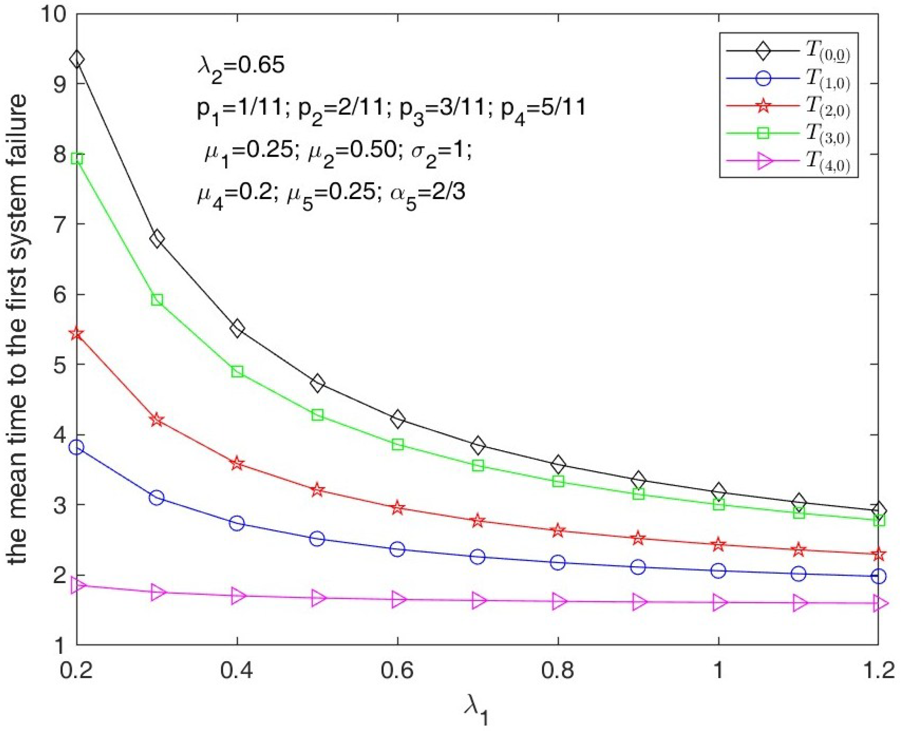
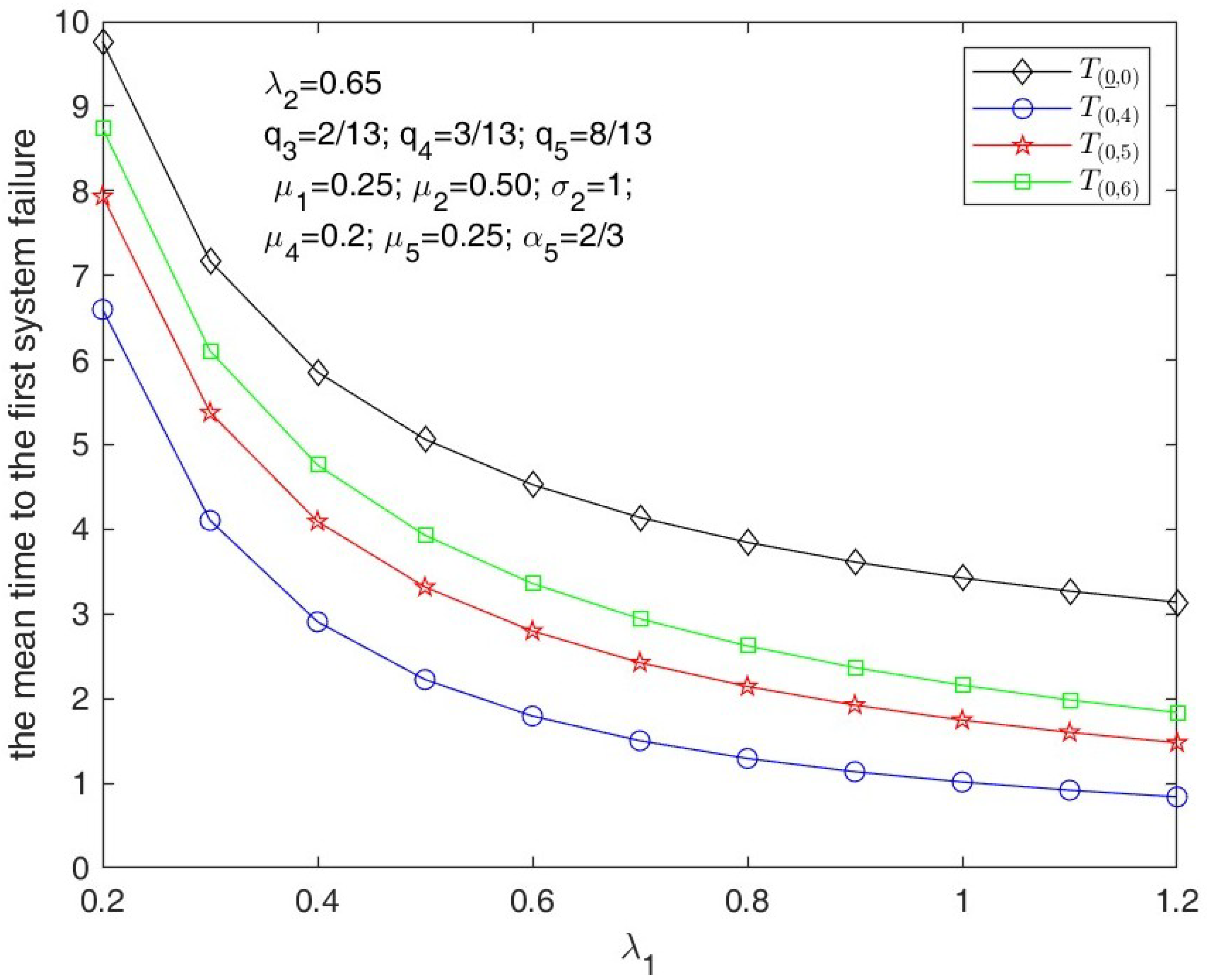
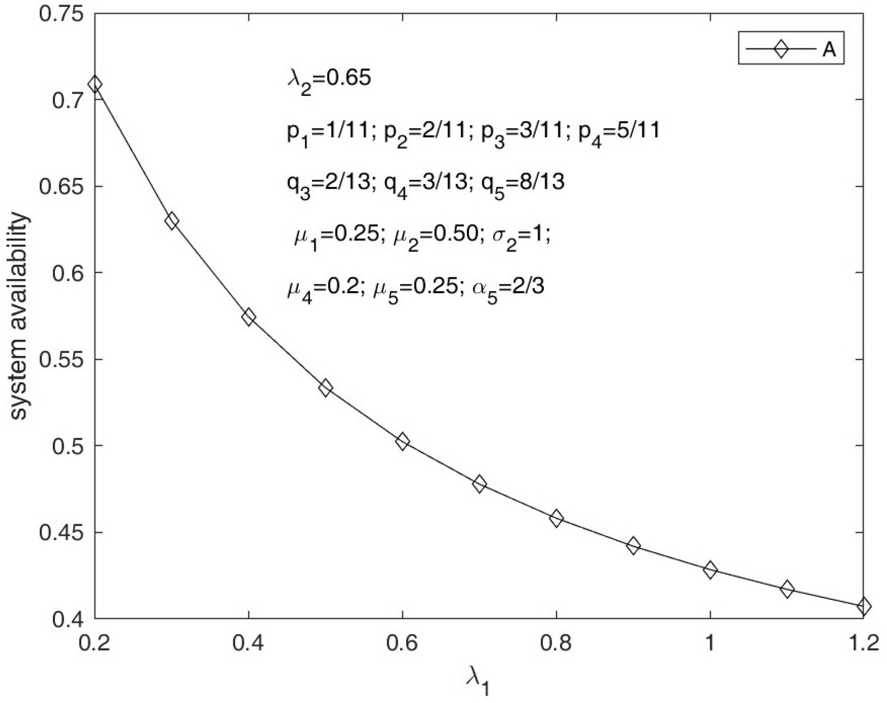
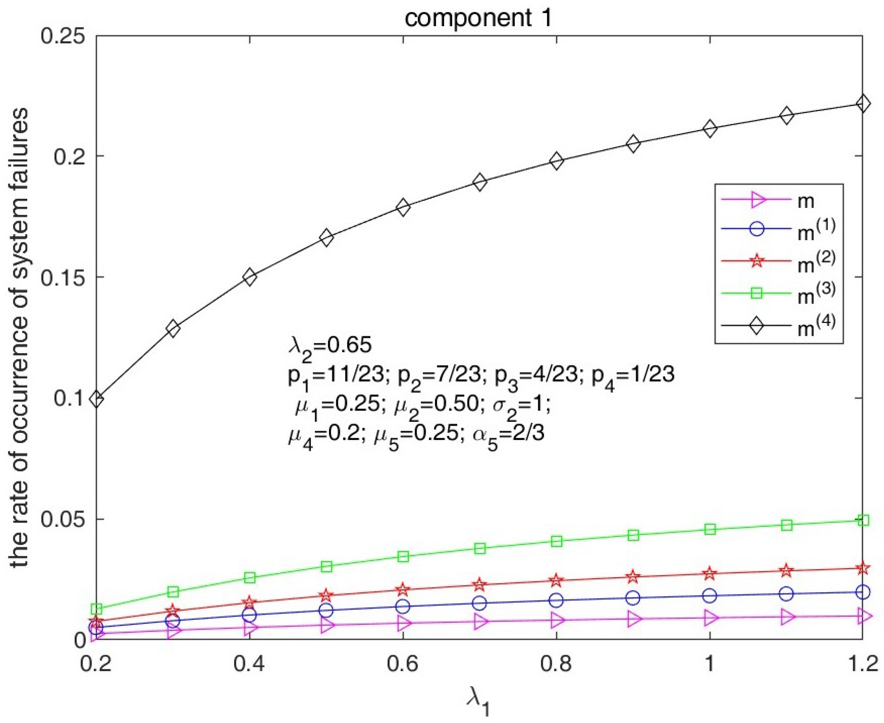
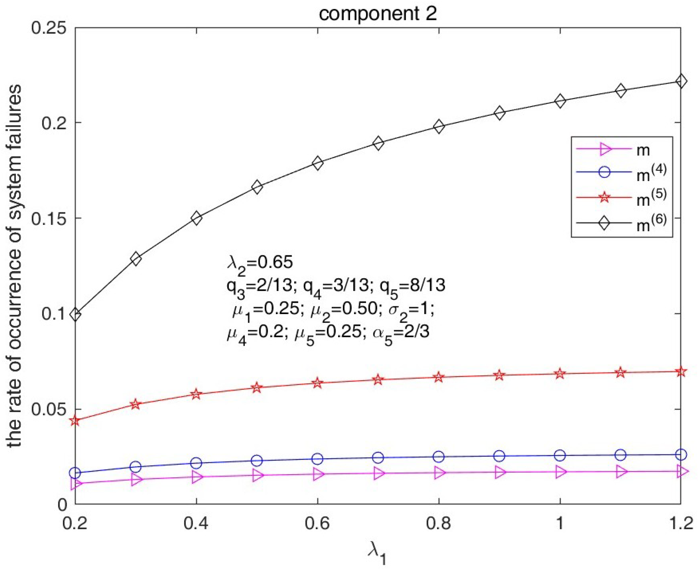
For example, the failure probability of component 1 is set to be $p=(p_1,p_2,p_3,p_4,p_5,p_6)$$=({\displaystyle \frac{1}{11}},{\displaystyle \frac{2}{11}},{\displaystyle \frac{3}{11}},{\displaystyle \frac{5}{11}},0,0)$, and the failure probability of component 2 is set to be $q=(q_1,q_2,q_3,q_4,q_5,q_6)=(0,0,0,{\displaystyle \frac{2}{13}},{\displaystyle \frac{3}{13}},{\displaystyle \frac{8}{13}})$. We select repair rates ${\mu }_1=0.25$, ${\mu }_2=0.50,\delta =1$, ${\mu }_4=0.2$, gamma parameters ${\alpha }_5=2/3,{\mu }_5=0.75$, and failure rate ${\lambda }_2=0.65$. The parameter ${\lambda }_1$ varies from $0.2$ to $1.2$. Numerical results are listed in

Table 2. The mean time to the first system failure under different initial conditions.

${\mathit{\lambda }}_1$	0.2	0.3	0.4	0.5	0.6	0.7	0.8	0.9	1.0	1.1	1.2
$T_{(0,\underline{0})}$	9.343	6.793	5.512	4.741	4.225	3.854	3.575	3.357	3.182	3.038	2.918
$T_{(1,0)}$	3.822	3.103	2.739	2.518	2.369	2.261	2.179	2.115	2.063	2.019	1.983
$T_{(2,0)}$	5.442	4.212	3.590	3.212	2.958	2.774	2.634	2.524	2.434	2.360	2.298
$T_{(3,0)}$	7.927	5.914	4.896	4.278	3.861	3.560	3.331	3.151	3.005	2.884	2.782
$T_{(4,0)}$	1.857	1.757	1.706	1.675	1.654	1.639	1.628	1.619	1.612	1.606	1.601
$T_{(\underline{0},0)}$	9.760	7.169	5.859	5.064	4.528	4.140	3.846	3.614	3.426	3.270	3.138
$T_{(0,4)}$	6.598	4.105	2.908	2.225	1.794	1.502	1.293	1.136	1.015	0.918	0.838
$T_{(0,5)}$	7.935	5.378	4.093	3.318	2.798	2.425	2.143	1.923	1.746	1.601	1.479
$T_{(0,6)}$	8.735	6.107	4.759	3.929	3.360	2.943	2.622	2.367	2.158	1.984	1.836

and

Table 3. The steady-state availability and the rate of occurrence of system failure.

${\mathit{\lambda }}_1$	0.2	0.3	0.4	0.5	0.6	0.7	0.8	0.9	1.0	1.1	1.2
A	0.709	0.630	0.575	0.534	0.502	0.478	0.458	0.442	0.429	0.417	0.407
m	0.099	0.1287	0.150	0.1663	0.179	0.1893	0.198	0.2052	0.211	0.2169	0.222
$m^{\left(1\right)}|{\sigma }_1$	0.003	0.004	0.005	0.006	0.007	0.008	0.008	0.009	0.009	0.010	0.010
$m^{\left(2\right)}|{\sigma }_1$	0.005	0.008	0.010	0.012	0.014	0.015	0.016	0.017	0.018	0.019	0.020
$m^{\left(3\right)}|{\sigma }_1$	0.008	0.012	0.015	0.018	0.021	0.023	0.024	0.026	0.027	0.029	0.030
$m^{\left(4\right)}|{\sigma }_1$	0.013	0.020	0.026	0.030	0.034	0.038	0.041	0.043	0.046	0.048	0.049
$m^{\left(4\right)}|{\sigma }_2$	0.011	0.013	0.014	0.015	0.016	0.016	0.017	0.017	0.017	0.017	0.017
$m^{\left(5\right)}|{\sigma }_2$	0.016	0.020	0.022	0.023	0.024	0.024	0.025	0.025	0.026	0.026	0.026
$m^{\left(6\right)}|{\sigma }_2$	0.044	0.052	0.058	0.061	0.064	0.065	0.067	0.068	0.068	0.069	0.070

, while graphical illustrations are provided in Figure 3, Figure 4, Figure 5, Figure 6 and Figure 7.

Through the calculations, the following expected repair times, $E\left[Y_1\right]=4$, $E\left[Y_2\right]=2$, $E\left[Y_3\right]=0.4374$, $E\left[Y_4\right]=5$, $E\left[Y_5\right]=2.6667$ and $E\left[Y_6\right]=0.793$, can be derived. The relationships $E\left[Y_1\right]>E\left[Y_2\right]>E\left[Y_3\right]$ and $E\left[Y_4\right]>E\left[Y_5\right]>E\left[Y_6\right]$ indicate that repair times for failed components vary significantly across different failure modes.

As shown in Table 2 and Figure 3 and Figure 4, we observe the following relationships:

$$T(0,\underline{0})>T(3,0)>T(2,0)>T(1,0)>T(4,0),$$

and

$$T(\underline{0},0)>T(0,6)>T(0,5)>T(0,4).$$

These results indicate that shorter repair times correspond to longer system operational durations.

From Table 3 and Figure 5 and Figure 7, it can be seen that the system’s steady-state availability decreases as the component failure rate increases, whereas the rate of occurrence of system failures gradually increases. Due to the varying probabilities associated with different failure modes, the rates of occurrence of system failures also differ.

Example 2.

The analytical expressions for these steady-state reliability metrics depend solely on the Laplace–Stieltjes transform and the mean of the repair time distributions and are independent of variance. To investigate the impact of different distributions with the same mean on the main performance measures, we present a numerical example in which the repair time distribution is modeled using four distinct types, namely, exponential distribution (EXP), Erlangian distribution (ERL), Coxian distribution (COX), and Hyper-exponential distribution (HEX). The four distributions share the same mean but differ in their functional forms, which are provided below.

• Case 1: Exponential distribution (EXP)

  $${\mathit{\alpha }}_3=\left(1\right),{\mathbf{T}}_3=(-5),{\mathbf{T}}_3^0=(-5).$$
• Case 2: Erlangian distribution (ERL)

  $${\mathit{\alpha }}_3=(1,0,0),{\mathbf{T}}_3=\left(\begin{array}{ccc}-15& 15& 0\\ 0& -15& 15\\ 0& 0& -15\end{array}\right),{\mathbf{T}}_3^0=\left(\begin{array}{c}0\\ 0\\ 15\end{array}\right).$$
• Case 3: Coxian distribution (COX)

  $${\mathit{\alpha }}_3=(1,0),{\mathbf{T}}_3=\left(\begin{array}{cc}-15& 6\\ 0& -3\end{array}\right),{\mathbf{T}}_3^0=\left(\begin{array}{c}9\\ 3\end{array}\right).$$
• Case 4: Hyper-exponential distribution (HEX)

  $${\mathit{\alpha }}_3=(0.7,0.3),{\mathbf{T}}_3=\left(\begin{array}{cc}-10.5& 0\\ 0& -2.25\end{array}\right),{\mathbf{T}}_3^0=\left(\begin{array}{c}10.5\\ 2.25\end{array}\right).$$

The remaining parameters are set identically to those in Example 1. We know that all the repair time distributions are characterized by a mean repair time equal to 0.2, and the corresponding computational results are provided in

Table 4. The steady-state reliability measures under different repair time distributions.

	$\mathit{\lambda }=0.2$				$\mathit{\lambda }=0.4$
$T_{(0,\underline{0})}$	9.677	9.662	9.693	9.699	5.676	5.669	5.684	5.687
$T_{(1,0)}$	3.891	3.888	3.894	3.896	2.766	2.765	2.768	2.768
$T_{(2,0)}$	5.559	5.554	5.565	5.567	3.637	3.635	3.639	3.640
$T_{(3,0)}$	9.033	8.986	9.089	9.107	5.450	5.426	5.477	5.486
$T_{(4,0)}$	1.867	1.866	1.867	1.867	1.710	1.710	1.710	1.710
$T_{(\underline{0},0)}$	10.008	9.997	10.020	10.024	5.958	5.954	5.963	5.965
$T_{(0,4)}$	6.720	6.715	6.727	6.729	2.930	2.929	2.931	2.931
$T_{(0,5)}$	8.160	8.151	8.172	8.176	4.180	4.176	4.184	4.186
$T_{(0,6)}$	9.022	9.010	9.036	9.041	4.882	4.877	4.888	4.890
A	0.710	0.710	0.710	0.710	0.576	0.576	0.576	0.576
m	0.096	0.097	0.096	0.096	0.146	0.146	0.146	0.146

. To present the differences in numerical results more intuitively, we only display results for $\lambda =0.2$ and $\lambda =0.4$, as seen in Table 4.

The observed differences in system performance metrics are primarily due to the distinct Laplace–Stieltjes transforms of the repair time distributions. These transforms capture not only the mean but also the shape characteristics and variability of the repair process. Even with identical means, different distributional forms lead to differences in steady-state system behavior, as demonstrated by the numerical results.

7. Conclusions

A cold standby repairable system comprising two types of components is investigated. Each component subjects to c distinct failure modes, while the repair times corresponding to different failure modes follow general distributions. By employing Markov renewal process theory, the Laplace transform, and the Laplace–Stieltjes transform, we derive the time-to-failure distribution function, the mean time to the first system failure, the steady-state system availability, and the rate of occurrence of system failures. Explicit analytical expressions for these reliability metrics are established. Numerical examples are presented under the assumption that component repair times follow exponential, inverse Gaussian, phase-type, deterministic, gamma, and Coxian distributions. The resulting reliability indicators are computed and analyzed to illustrate the theoretical results.

It should be noted that this study has certain limitations. Specifically, while the Laplace and Laplace–Stieltjes transforms of the relevant reliability metrics have been obtained, the inversion of these transforms to derive transient-state results has not been pursued, which is a research topic to be discussed in the future.

References

1. Coit, D.W. Cold–standby redundancy optimization for nonrepairable systems. IIE Trans. 2001, 33, 471–478. [Google Scholar] [CrossRef]
2. Zhang, Y.L.; Wang, G.J. A deteriorating cold standby repairable system with priority in use. Eur. J. Oper. Res. 2007, 183, 278–295. [Google Scholar] [CrossRef]
3. Jia, J.S.; Wu, S.M. Optimizing replacement policy for a cold–standby system with waiting repair times. Appl. Math. Comput. 2009, 214, 133–141. [Google Scholar] [CrossRef]
4. Leung, K.N.F.; Yuan, L.Z.; Lai, K.K. A bivariate optimal replacement policy for a cold standby repairable system with repair priority. Nav. Res. Log. 2010, 57, 149–158. [Google Scholar] [CrossRef]
5. Wu, Q.T.; Wu, S.M. Reliability analysis of two–unit cold standby repairable systems under Poisson shocks. Appl. Math. Comput. 2011, 218, 171–182. [Google Scholar] [CrossRef]
6. Eryilmaz, S. On the mean residual life of a k–out–of–n: G system with a single cold standby component. Eur. J. Oper. Res. 2010, 222, 273–277. [Google Scholar] [CrossRef]
7. Liu, B.; Cui, L.; Wen, Y. Cold standby repairable system with working vacations and vacations interruption. J. Syst. Sci. Complex. 2015, 26, 1127–1134. [Google Scholar] [CrossRef]
8. Liu, B.; Cui, L.; Wen, Y.; Shen, J. A cold standby repairable system with working vacations and vacation interruption following Markovian arrival process. Reliab. Eng. Syst. Saf. 2015, 142, 1–8. [Google Scholar] [CrossRef]
9. Liu, B.; Cui, L.; Wen, Y.; Guo, F. A cold standby repairable system with the repairman having multiple vacations and operational, repair, and vacation times following phase–type distributions. Commun. Stat.-Theory Methods 2016, 45, 850–858. [Google Scholar] [CrossRef]
10. Eryilmaz, S. The effectiveness of adding cold standby redundancy to a coherent system at system and component levels. Reliab. Eng. Syst. Saf. 2017, 165, 331–335. [Google Scholar] [CrossRef]
11. Yang, D.Y.; Tsao, C.L. Reliability and availability analysis of standby systems with working vacations and retrial of failed components. Reliab. Eng. Syst. Saf. 2019, 182, 46–55. [Google Scholar] [CrossRef]
12. EL–Sherbeny, M.S.; Mahmoud, M.A.W.; Hussien, Z.M. Reliability analysis of a two–unit cold standby system with arbitrary distributions and change in units. Life Cycle Reliab. Saf. Eng. 2020, 9, 261–272. [Google Scholar] [CrossRef]
13. Yang, D.Y.; Wu, C.H. Evaluation of the availability and reliability of a standby repairable system incorporating imperfect switchovers and working breakdowns. Reliab. Eng. Syst. Saf. 2021, 207, 107366. [Google Scholar] [CrossRef]
14. Roy, A.; Gupta, N. Reliability function of k–out–of–n system equipped with two cold standby components. Commun. Stat.-Theory Methods 2021, 50, 5759–5778. [Google Scholar] [CrossRef]
15. Roy, A.; Gupta, N. A study on utilization of two cold standby components to increase reliability of a coherent system. Commun. Stat.-Theory Methods 2025, 54, 324–351. [Google Scholar] [CrossRef]
16. Ma, M.R.; Hu, L.M.; Wang, Y.Y.; Luo, F. Discrete–time stochastic modeling and optimization for reliability systems with retrial and cold standbys. AIMS Math. 2024, 9, 19692–19717. [Google Scholar] [CrossRef]
17. Juybari, M.N.; Hamadani, A.Z.; Ardakan, M.A. Availability analysis and cost optimization of a repairable system with a mix of active and warm standby components in a shock environment. Reliab. Eng. Syst. Saf. 2023, 237, 109375. [Google Scholar] [CrossRef]
18. Ragheb, N.M.; Solouma, E.; Alahmari, A.A.; Saber, S. Reliability and availability analysis of a two–unit cold standby system with imperfect switching. Axioms 2025, 14, 589. [Google Scholar] [CrossRef]
19. Mendes, A.A.; Ribeiro, J.L.D.; Coit, D.W. Optimal time interval between periodic inspections for a two–component cold standby multistate system. IEEE Trans. Reliab. 2017, 66, 559–574. [Google Scholar] [CrossRef]
20. Chen, Y.; Wang, Z.; Li, Y.Y.; Kang, R.; Mosleh, A. Reliability analysis of a cold–standby system considering the development stages and accumulations of failure mechanisms. Reliab. Eng. Syst. Saf. 2018, 180, 1–12. [Google Scholar] [CrossRef]
21. Qi, F.Q.; Zhou, B.H. Maintenance policy optimization for a cold standby system considering multiple failure types. J. Qual. Maint. Eng. 2019, 25, 182–198. [Google Scholar] [CrossRef]
22. Wang, J.T.; Xie, N.; Yang, N. Reliability analysis of a two–dissimilar–unit warm standby repairable system with priority in use. Commun. Stat.-Theory Methods 2021, 50, 792–814. [Google Scholar] [CrossRef]
23. Hu, L.; Liu, S.; Peng, R.; Liu, Z. Reliability and sensitivity analysis of a repairable k–out–of–n: G system with two failure modes and retrial feature. Commun. Stat.-Theory Methods 2022, 51, 3043–3064. [Google Scholar] [CrossRef]
24. Li, J.; Hu, L.; Wang, Y.; Kang, J. Reliability analysis and optimization design of a repairable k–out–of–n retrial system with two failure modes and preventive maintenance. Commun. Stat.-Theory Methods 2024, 53, 5524–5552. [Google Scholar] [CrossRef]
25. Qiu, Q.A.; Cui, L.R.; Gao, H.D. Availability and maintenance modelling for systems subject to multiple failure modes. Comput. Ind. Eng. 2017, 108, 192–198. [Google Scholar] [CrossRef]
26. Liu, P.; Wang, G. Optimal preventive maintenance policies for products with multiple failure modes after geometric warranty expiry. Commun. Stat.-Theory Methods 2023, 52, 8794–8813. [Google Scholar] [CrossRef]
27. Liu, L.L.; Ai, X.C.; Wu, J. Reliability and residual life of cold standby systems. Mathematics 2024, 12, 1540. [Google Scholar] [CrossRef]
28. Khati, A.; Chantola, N.; Singh, S.B. Availability modeling of systems incorporating uncertainty & multiple failure modes using critical repair time & copula. Commun. Stat.-Theory Methods 2024, 53, 595–609. [Google Scholar]
29. Wu, W.Q.; He, Y.X.; Kuang, X.Y.; Lan, S.J.; Liu, J.Y. The reliability of a two identical components cold standby system with replaceable repair equipment and multiple failure modes. J. Intell. Manag. 2025, 1, 43–50. [Google Scholar] [CrossRef]
30. Wu, W.Q.; Xu, H.W.; Zheng, K.L.; Yu, M.M.; He, Y.X. Reliability analysis of a two identical components cold standby system with multiple failure modes. Commun. Stat.-Theory Methods 2026, 55, 5499–5569. [Google Scholar] [CrossRef]
Figure 1. The schematic diagram of the proposed reliability system.
Axioms 15 00251 g001
Figure 2. The state transition diagram of the system.
Axioms 15 00251 g002
Figure 3. The mean time to the first system failure under initial condition ( 0 , 0 ̲ ) and ( ϑ 1 , 0 ) , ϑ 1 = 1 , 2 , 3 , 4 .
Axioms 15 00251 g003
Figure 4. The mean time to the first system failure under initial condition ( 0 ̲ , 0 ) and ( 0 , ϑ 2 ) , ϑ 2 = 4 , 5 , 6 .
Axioms 15 00251 g004
Figure 5. The steady-state system availability.
Axioms 15 00251 g005
Figure 6. The rate of occurrence of system failures caused by the σ 1 -type failure.
Axioms 15 00251 g006
Figure 7. The rate of occurrence of system failures caused by the σ 2 -type failure.
Axioms 15 00251 g007