Exploring Nonlinear Dynamics of the (3+1)-Dimensional Boussinesq-Type Equation: Wave Patterns and Sensitivity Insight

Abstract

This study examines a nonlinear partial differential equation, namely the (3+1)-dimensional Boussinesq-type equation. To explore this model, three versatile analytical approaches are applied: the Exp-function method, the Kudryashov method, and the Riccati equation method. Using these techniques, a range of exact analytical solutions is derived, exhibiting diverse structural forms such as periodic, kink-type, rational, and trigonometric solutions. The analysis reveals the rich dynamical behavior of the equation and demonstrates its effectiveness in modeling a variety of nonlinear wave phenomena across different physical contexts. Several of the obtained solutions are illustrated through graphical representations for better interpretation. The results include hyperbolic, trigonometric, and rational function solutions, along with a sensitivity analysis. To highlight the physical relevance of the findings, suitable parameter values are selected, and the corresponding wave behaviors are visualized using three-dimensional and contour plots generated with Maple 2024. Overall, the study provides valuable insights into the mechanisms underlying the generation and propagation of complex nonlinear phenomena in fields such as fluid dynamics, optical fiber systems, plasma physics, and ocean wave transmission.

1. Introduction

With a wide range of engineering and physical applications, nonlinear evolution equations (NLEEs) and systems have constituted an intriguing area of research and modeling. They have provided a strong basis for comprehending the complex dynamics of some natural nonlinear phenomena [1]. They have served as the foundation for modern science’s understanding of such concepts as those in quantum mechanics, general relativity, electrostatics, electrodynamics, elasticity, heat, sound, and diffusion [2]. The NLEEs have evolved into the essential instruments for the modeling and analysis of various nonlinear phenomena in both the laboratory and the natural world [3]. The essential characteristics of nonlinear waves, such as solitons and their interactions, rogue waves, and numerous complex progressive processes, are entirely encompassed within these equations, often expressed as partial differential equations (PDEs) [4,5]. A wide variety of complicated events spanning several scientific areas have been mostly described by the nonlinear partial differential equations (NLPDEs) [6]. Their importance has been derived from their ability to represent the complex behaviors which the linear equations are frequently unable to present accurately [7]. Furthermore, the formation and propagation of the shock waves, solitary waves, cnoidal waves [8], their interplays with the barriers, as well as stability of the wave patterns have all been greatly aided by those equations [9,10]. By offering the precise forecasts of light-pulse propagation in optical fibers, integrable NLEEs have substantially influenced optics [11]. Those equations have improved the comprehension of soliton propagation, a critical attribute of contemporary optical-communication systems [12]. They have become the indispensable instruments for investigating and forecasting the complex systems in numerous scientific disciplines due to their capacity to comprehend the fundamental attributes of nonlinear processes [13]. Their capacity to yield a profound comprehension about the underlying characteristics of nonlinear systems and their wide-ranging applications has guaranteed their lasting importance in developing the scientific knowledge [14]. Solitons are the waves that are confined to a certain region and occur and travel in different nonlinear and dispersive media [15]. Those waves are distinct from the conventional waves that propagate over the time and ultimately dissipate [16]. Solitons possess the unique quality of retaining their form, velocity, and inherent characteristics after collisions with other solitons [17]. The existence of solitons may be seen in a broad variety of physical phenomena, including plasma, optics, fluid mechanics, acoustics, hydrodynamics, and ocean waves, which demonstrates their pervasiveness [14]. A wide range of potent techniques has been developed to investigate and solve NLEEs. These techniques encompass the Backlund transformation approach [18], the modified auxiliary equation approach [19], the extended simple equation approach [20], the modified exp-function approach [21], homogeneous balance approach [22], the tanh method [23], the modified extended tanh function method [24], the exponential rational function approach [25], bifurcation and chaos [26] and numerous others [27]. Numerous solutions for nonlinear models, including kink solutions, solitons solutions, rogue waves, hyperbolic solutions, breathers, lumps, periodic solutions, and many more, have been found using these approaches.

In 1871, Joseph Boussinesq developed the BE, which depicts the features of shallow water waves with small amplitude that propagate with constant speed in a water channel. The BE equation is expressed as

$$u_{tt}-u_{xxxx}-u_{xx}-3{\left(u^2\right)}_{xx}=0.$$

(1)

Here $u=u(x,t)$ is a real-valued function that represents the height of a fluid’s free surface, with subscripts indicating partial derivatives [28,29]. Since then, it has been applied to a wide variety of circumstances, such as the study of different acoustic waves and oscillations in plasma, water percolation in porous materials, and vibrations in nonlinear strings. The significance of the BE is underscored by its applicability to various phenomena, such as tsunami wave propagation, coastal harbor dynamics, and ocean beach behavior [30,31]. Additionally, researchers have put forward and thoroughly examined several extended forms of the BE, resulting in significant discoveries across multiple domains. The following novel (3+1)-dimensional Boussinesq-type equation is presented in this work [14]:

$$u_{tt}-u_{xxxx}+u_{xx}+u_{xt}+u_{xy}+u_{xz}+u_x{u}_{xx}=0.$$

(2)

Here $u=u(x,y,z,t)$. The (3+1)-dimensional Boussinesq-type equation is an extended form of the conventional BE, used to examine the dissemination of extended waves in shallow water and other fluid media. Equation (2) is derived by substituting the nonlinear term ${\left(u^2\right)}_{xx}$ in Equation (1) with the nonlinear term $u_x{u}_{xx}$. Additionally, three linear terms, specifically $u_{xt}$, $u_{xy}$, $u_{xz}$, were incorporated into Equation (1) to extend it to the (3+1)-dimensional model. The additional linear terms $u_{xt}$, $u_{xy}$, and $u_{xz}$ represent space–time coupling and transverse spatial interactions. Specifically, $u_{xt}$ models the convective or transport effects along the primary propagation direction, while $u_{xy}$ and $u_{xz}$ account for multidimensional coupling between longitudinal and transverse spatial components. These terms introduce anisotropic dispersion and enable the equation to describe fully three-dimensional wave propagation phenomena observed in fluid dynamics, nonlinear optics, and plasma systems. The essential characteristic of this novel model resides in the balance between the dispersive effects of the linear term $u_{xxxx}$ and the nonlinear term $u_x{u}_{xx}$. This equation is applicable for describing phenomena such as nonlinear optics, multidimensional wave propagation in fluids, and other physical systems where the interaction between nonlinearity and dispersion is essential. The formation of solitons is a direct consequence of this balance. Multiple research works have been carried out on the (3+1)-dimensional Boussinesq-type equation, resulting in diverse findings. The integrability was examined by using the Painleve test, and the Hirota bilinear technique was employed to get soliton solutions to the (3+1)-dimensional Boussinesq-type equation [14], Lump solutions were obtained by using the long-wave limit method [32].

In 2024 Hajar F. Ismael et al. [2] studied the (3+1)-dimensional Boussinesq-type equation by using the Hirota method and discussed the variety of multiple solitons and M-lump solutions. A stationary mass transfer model was developed, extending the Boussinesq approximation with variable coefficients influenced by concentration and spatial variables, and subsequently studied [33]. An innovative non-trivial precise solution to the steady-state thermal diffusion equations for shear flows of a binary incompressible fluid was developed inside the Lin–Sidorov–Aristov class under the Oberbeck–Boussinesq framework [34]. An optical control problem is discussed through generalized Boussinesq [35], and another study is discussed here [36]. The novelty of this investigation lies in the (3+1)-dimensional Boussinesq-type equation that was used to obtain exact solutions. To this end, we made use of the recently developed analytical methods such as the exp-part method, the new Kudryashov method, and the Riccati equation method. By applying such approaches we were able to obtain new solutions of kink and anti-kink solitons, which were not obtained for this model. Furthermore, a sensitivity analysis was performed to study the wave solution behavior with different initial conditions. Here is a brief overview of the paper: Section 2 provides an overview of the method. Section 3 discusses solutions of the (3+1)-dimensional Boussinesq-type equation exactly. In Section 4 and Section 5, we briefly discuss the results, as well as the analysis of the obtained solutions. The sensitivity of the model and the obtained solutions are discussed in Section 6. Finally, the conclusion is provided in the last part.

2. Description of the Methodologies

Given an NLPDE of the following form for the unknown function $u(x,t)$:

$$\Omega (u,u_t,u_x,u_y,u_z,u_{xy},u_{xz},u_{yz},u_{tt},u_{xx},\dots )=0.$$

(3)

By implementing the transformation

$$\begin{array}{c}\hfill u(x,y,z,t)=U\left(\rho \right),\rho =x+a_{1}y+a_{2}z-a_{3}t.\end{array}$$

(4)

where $\sigma$ indicates the speed of wave.

Equation (3) can be converted into an ODE of the form

$$G(U,U_{\rho },U_{\rho \rho },U_{\rho \rho \rho },\dots )=0.$$

(5)

2.1. Exp-Expansion Method

The basic solution related to these strategies is described as follows:

$$U\left(\rho \right)=\sum _{i=0}^N{A}_i{V}^i\left(\rho \right),A_i\ne 0·$$

(6)

The balance principle in Equation (5) must be used to get the number N. The following is how the function $V\left(\rho \right)$ satisfies the first-order differential equation:

$$V^{\prime }\left(\rho \right)=\exp (-V\left(\rho \right))+S\exp \left(V\left(\rho \right)\right)+R,$$

(7)

where S and R are constants.

The corresponding solutions of Equation (7) can be seen as

$$V\left(\rho \right)=\left\{\begin{array}{cc}\hfill & \ln \left[-{\displaystyle \frac{R}{2S}}-{\displaystyle \frac{\sqrt{\mu }}{2S}}\tanh \left({\displaystyle \frac{\sqrt{\mu }}{2}}(\rho -{\rho }_0)\right)\right],S\ne 0,\mu >0\hfill \\ \hfill & \ln \left[-{\displaystyle \frac{R}{2S}}-{\displaystyle \frac{\sqrt{\mu }}{2S}}\coth \left({\displaystyle \frac{\sqrt{\mu }}{2}}(\rho -{\rho }_0)\right)\right],S\ne 0,\mu >0,\hfill \\ \hfill & \ln \left[-{\displaystyle \frac{R}{2S}}+{\displaystyle \frac{\sqrt{-\mu }}{2S}}\tan \left({\displaystyle \frac{\sqrt{-\mu }}{2}}(\rho -{\rho }_0)\right)\right],S\ne 0,\mu <0,\hfill \\ \hfill & \ln \left[-{\displaystyle \frac{R}{2S}}-{\displaystyle \frac{\sqrt{-\mu }}{2S}}\cot \left({\displaystyle \frac{\sqrt{-\mu }}{2}}(\rho -{\rho }_0)\right)\right],S\ne 0,\mu <0\hfill \end{array}\right.$$

(8)

where $\mu =R^2-4S$, and ${\rho }_0$ is an arbitrary constant.

2.2. Kudryashov Method

Consider that (5) has the solution

$$U\left(\rho \right)=A_0+A_{1}V\left(\rho \right)+A_2{V}^2\left(\rho \right)+\cdots +A_N{V}^N\left(\rho \right),$$

(9)

where $A_i,(i=0,1,\dots ,N)$ are the coefficients corresponding to $V^i\left(\rho \right)$ with $A_N\ne 0$ and $V\left(\rho \right)$ satisfying the first-order differential equation as follows:

$$V^{\prime }\left(\rho \right)=V^2\left(\rho \right)-V\left(\rho \right).$$

(10)

The solutions of (10) can be written as

$$V\left(\rho \right)={\displaystyle \frac{1}{1+e^{\rho }}}.$$

(11)

Here, N will be determined by employing the classical balance principle on Equation (5) then be inserted into Equation (9). The procedure described above allows us to find the values of $A_i$ by comparing the coefficients of $V\left(\rho \right)$ to zero. Once these values are determined, we can obtain solutions using the explicit strategy and with the help of parameters. Finally, by switching $\rho =x+a_{1}y+a_{2}z-a_{3}t.$ into the solutions satisfying (5), we can conclude the procedure.

2.3. Description of the Riccati Equation Method

Using the Riccati equation approach, the answer to (5) is as follows:

$$\begin{array}{c}\hfill U\left(\rho \right)=\sum _{i=0}^N{\mathcal{C}}_i{V}^i\left(\rho \right),\end{array}$$

(12)

where the function $V\left(\rho \right)$ satisfies the first-order differential Riccati equation as follows, and ${\mathcal{C}}_0,{\mathcal{C}}_1$ and ${\mathcal{C}}_2$ are unknown real parameters:

$$V^{\prime }\left(\rho \right)={\mathcal{D}}_0+{\mathcal{D}}_{1}V\left(\rho \right)+{\mathcal{D}}_2{V}^2\left(\rho \right).$$

(13)

where ${\mathcal{D}}_0,{\mathcal{D}}_1$ and ${\mathcal{D}}_2$ are real constants.

The solutions of (13) are

$$V\left(\rho \right)=\left\{\begin{array}{cc}\hfill & -{\displaystyle \frac{{\mathcal{D}}_1}{2{\mathcal{D}}_2}}-{\displaystyle \frac{\sqrt{\Phi }}{2{\mathcal{D}}_2}}\tanh \left({\displaystyle \frac{\sqrt{\Phi }}{2}}(\rho +{\rho }_0)\right),\Phi >0,\hfill \\ \hfill & -{\displaystyle \frac{{\mathcal{D}}_1}{2{\mathcal{D}}_2}}-{\displaystyle \frac{\sqrt{\Phi }}{2{\mathcal{D}}_2}}\coth \left({\displaystyle \frac{\sqrt{\Phi }}{2}}(\rho +{\rho }_0)\right),\Phi >0,\hfill \\ \hfill & -{\displaystyle \frac{{\mathcal{D}}_1}{2{\mathcal{D}}_2}}+{\displaystyle \frac{\sqrt{-\Phi }}{2{\mathcal{D}}_2}}\tan \left({\displaystyle \frac{\sqrt{-\Phi }}{2}}(\rho +{\rho }_0)\right),\Phi <0,\hfill \\ \hfill & -{\displaystyle \frac{{\mathcal{D}}_1}{2{\mathcal{D}}_2}}-{\displaystyle \frac{\sqrt{-\Phi }}{2{\mathcal{D}}_2}}\cot \left({\displaystyle \frac{\sqrt{-\Phi }}{2}}(\rho +{\rho }_0)\right),\Phi <0,\hfill \\ \hfill & -{\displaystyle \frac{{\mathcal{D}}_1}{2{\mathcal{D}}_2}}-{\displaystyle \frac{1}{{\mathcal{D}}_2(\rho +{\rho }_0)}},\Phi =0.\hfill \end{array}\right.$$

(14)

where $\Phi ={\mathcal{D}}_1^2-4{\mathcal{D}}_0{\mathcal{D}}_2$.

Here, N will be determined by employing the classical balance principle, and Equation (9) will then be inserted into Equation (5). The procedure described above allows us to find the values of a, b, and $c_i$ by comparing the coefficients of $V^i\left(\rho \right)$ to zero. Once these values are determined, we can obtain solutions using the explicit strategy and the help of parameters. Finally, by switching $\rho =x+a_{1}y+a_{2}z-a_{3}t$ into the solutions satisfying (5), we can conclude the procedure.

3. Solitary Wave Solutions of Equation (2)

Consider the wave transformation

$$u(x,y,z,t)=U\left(\rho \right),\rho =x+a_{1}y+a_{2}z-a_{3}t.$$

(15)

Putting Equation (15) into Equation (2) reduces into the following form:

$$U^{⁗}-U^{\prime }{U}^{″}-\left(a_3^2+a_1+a_2-a_3+1\right)U^{″}=0,$$

(16)

where $(\prime )$ represents the derivative with respect to $\rho$. Integrating (16), we have

$$2U^{‴}-{\left(U^{\prime }\right)}^2-2\left(a_3^2+a_1+a_2-a_3+1\right)U^{\prime }=0.$$

(17)

3.1. Solutions via Exp-Expansion Method

In this section, the (3+1)-dimensional Boussinesq-type equation is solved by the $exp(-V(\rho \left)\right)$-expansion method. The $exp(-V(\rho \left)\right)$-expansion method suggests the solution of Equation (17) is of the form

$$U\left(\rho \right)=A_0+A_{1}exp(-V\left(\rho \right)),$$

(18)

where $A_0$ and $A_1$ are arbitrary constants, and $A_1\ne 0$. By substituting Equation (18) and Equation (7) into Equation (17), and equating the different power of $exp(-V(\rho \left)\right)$ to zero, we obtain the system of equations

$$\left.\begin{array}{c}{A}_{1}RS+R^3-R{a}_3^2+8RS-R{a}_1-R{a}_2+R{a}_3-R=0,\hfill \\ S{R}^2-S{a}_3^2-S{a}_2+S{a}_3+{\displaystyle \frac{1}{2}}{S}^2{A}_1-S{a}_1-S+2S^2=0,\hfill \\ S{A}_1+{\displaystyle \frac{1}{2}}{R}^2{A}_1+8S+7R^2-a_3^2-a_1-a_2+a_3-1=0,\hfill \\ A_{1}R+12R=0,\hfill \\ 6+{\displaystyle \frac{A_1}{2}}=0.\hfill \end{array}\right\}$$

(19)

By using the Maple software, we solve the system of equations and get the following set of solutions.

• Set1:

  $$\left[A_0=A_0,A_1=-12,a_3={\displaystyle \frac{1}{2}}+{\displaystyle \frac{\sqrt{4R^2-16S-4a_1-4a_2-3}}{2}}\right]$$

  (20)

By inserting Equation (20) into Equation (19), we get the solution of Equation (1) as

• Case1: when $\mu >0$ then

  $$u_1(x,y,z,t)=A_0-{\displaystyle \frac{12}{\left[-\frac{R}{2S}-\frac{\sqrt{R^2-4S}tanh\left(\sqrt{R^2-4S}\left(\frac{a_{1}y+a_{2}z-\left(\frac{1}{2}+\frac{\sqrt{4R^2-16S-4a_1-4a_2-3}}{2}\right)t+x}{2}\right)\right)}{2S}\right]}}$$

  (21)

• Case2: when $\mu >0$ then

  $$u_2(x,y,z,t)=A_0-{\displaystyle \frac{12}{\left[-\frac{R}{2S}-\frac{\sqrt{R^2-4S}coth\left(\sqrt{R^2-4S}\left(\frac{a_{1}y+a_{2}z-\left(\frac{1}{2}+\frac{\sqrt{4R^2-16S-4a_1-4a_2-3}}{2}\right)t+x}{2}\right)\right)}{2S}\right]}}$$

  (22)

• Case3: when $\mu <0$ then

  $$u_3(x,y,z,t)=A_0-{\displaystyle \frac{12}{\left[-\frac{R}{2S}+\frac{\sqrt{-R^2+4S}tan\left(\sqrt{-R^2+4S}\left(\frac{a_{1}y+a_{2}z-\left(\frac{1}{2}+\frac{\sqrt{4R^2-16S-4a_1-4a_2-3}}{2}\right)t+x}{2}\right)\right)}{2S}\right]}}$$

  (23)

• Case4: when $\mu <0$ then

  $$u_4(x,y,z,t)=A_0-{\displaystyle \frac{12}{\left[-\frac{R}{2S}-\frac{\sqrt{-R^2+4S}cot\left(\frac{\sqrt{-R^2+4S}\left(a_{1}y+a_{2}z-\left(\frac{1}{2}+\frac{\sqrt{4R^2-16S-4a_1-4a_2-3}}{2}\right)t+x\right)}{2}\right)}{2S}\right]}}$$

  (24)

3.2. Solutions via Kudryashov Method

The new Kudryashov method suggests the solution of Equation (9) is of the form

$$U\left(\rho \right)=A_0+A_{1}V\left(\rho \right),$$

(25)

where $A_0$ and $A_1$ are constants to be ascertained, with $A_1\ne 0$. By substituting Equation (25) and Equation (10) into Equation (17) and setting the various powers of $V\left(\rho \right)$ to zero, we derive the subsequent system of equations:

$$\left.\begin{array}{c}-2A_1+\left(2a_3^2+2a_1+2a_2-2a_3+2\right)A_1=0,\hfill \\ 14A_1-A_1^2-\left(2a_3^2+2a_1+2a_2-2a_3+2\right)A_1=0,\hfill \\ 2A_1^2-24A_1=0,\hfill \\ -A_1^2+12A_1=0.\hfill \end{array}\right\}$$

(26)

Solving the system of equations, we obtain the following set of solutions:

• $\mathbf{Set}\mathbf{1}$

  $$\left[A_0=A_0,A_1=12,a_3={\displaystyle \frac{1}{2}}+{\displaystyle \frac{\sqrt{1-4a_1-4a_2}}{2}}\right]$$

  (27)

By substituting Equation (27) into Equation (25), we obtain the solution of Equation (1) as

$$u_1(x,y,z,t)=A_0+{\displaystyle \frac{12}{1+exp\left(a_{1}y+a_{2}z-\left(\frac{1}{2}+\frac{\sqrt{1-4a_1-4a_2}}{2}\right)t+x\right)}}$$

(28)

3.3. Solution via Riccati Equation Method

By substituting Equation (28) into Equation (17) and setting the coefficients of identical powers of R to zero, we obtain the previously described system:

$$\left.\begin{array}{c}12{\mathcal{D}}_2^3{c}_1-{\mathcal{D}}_2^2{c}_1^2=0,\hfill \\ 24{\mathcal{D}}_1{\mathcal{D}}_2^2{c}_1-2{\mathcal{D}}_1{\mathcal{D}}_2{c}_1^2=0,\hfill \\ -2a_3^2{\mathcal{D}}_2{c}_1+16{\mathcal{D}}_0{\mathcal{D}}_2^2{c}_1-2{\mathcal{D}}_0{\mathcal{D}}_2{c}_1^2+14{\mathcal{D}}_1^2{\mathcal{D}}_2{c}_1-{\mathcal{D}}_1^2{c}_1^2-2a_1{\mathcal{D}}_2{c}_1\hfill \\ -2a_2{\mathcal{D}}_2{c}_1+2a_3{\mathcal{D}}_2{c}_1-2{\mathcal{D}}_2{c}_1=0,\hfill \\ -2a_3^2{\mathcal{D}}_1{c}_1+16{\mathcal{D}}_0{\mathcal{D}}_1{\mathcal{D}}_2{c}_1-2{\mathcal{D}}_0{\mathcal{D}}_1{c}_1^2+2{\mathcal{D}}_1^3{c}_1-2a_1{\mathcal{D}}_1{c}_1\hfill \\ -2a_2{\mathcal{D}}_1{c}_1+2a_3{\mathcal{D}}_1{c}_1-2{\mathcal{D}}_1{c}_1=0,\hfill \\ -2a_3^2{\mathcal{D}}_0{c}_1+4{\mathcal{D}}_0^2{\mathcal{D}}_2{c}_1-{\mathcal{D}}_0^2{c}_1^2+2{\mathcal{D}}_0{\mathcal{D}}_1^2{c}_1-2a_1{\mathcal{D}}_0{c}_1\hfill \\ -2a_2{\mathcal{D}}_0{c}_1+2a_3{\mathcal{D}}_0{c}_1-2{\mathcal{D}}_0{c}_1=0,\hfill \end{array}\right\}$$

(29)

By solving the system of equations simultaneously, one obtains the solution set:

• Set1:

  $$\left\{a_3={\displaystyle \frac{1}{2}}+{\displaystyle \frac{\sqrt{-16{\mathcal{D}}_0{D}_2+4{\mathcal{D}}_1^2-4a_1-4a_2-3}}{2}},c_0=c_0,c_1=12{\mathcal{D}}_2\right\}$$

  (30)

By inserting Equation (30) into Equation (28), we obtain the following solutions of Equation (1):

• $\mathbf{Case}\mathbf{1}$ When $\Phi >0$, then:

  $$u_1(x,y,z,t)=c_0+12{\mathcal{D}}_2\left[{\displaystyle \frac{-{\mathcal{D}}_1}{2{\mathcal{D}}_2}}-{\displaystyle \frac{\sqrt{-4{\mathcal{D}}_0{\mathcal{D}}_2+{\mathcal{D}}_1^2}tanh\left(\sqrt{-4{\mathcal{D}}_0{\mathcal{D}}_2+{\mathcal{D}}_1^2}\frac{x+a_{1}y+a_{2}z-a_{3}t+{\rho }_0}{2}\right)}{2{\mathcal{D}}_2}}\right].$$

  (31)

• $\mathbf{Case}\mathbf{2}$ When $\Phi >0$, then:

  $$u_2(x,y,z,t)=c_0+12{\mathcal{D}}_2\left[{\displaystyle \frac{-{\mathcal{D}}_1}{2{\mathcal{D}}_2}}-{\displaystyle \frac{\sqrt{-4{\mathcal{D}}_0{\mathcal{D}}_2+{\mathcal{D}}_1^2}coth\left(\sqrt{-4{\mathcal{D}}_0{\mathcal{D}}_2+{\mathcal{D}}_1^2}\frac{x+a_{1}y+a_{2}z-a_{3}t+{\rho }_0}{2}\right)}{2{\mathcal{D}}_2}}\right].$$

  (32)

• $\mathbf{Case}\mathbf{3}$ When $\Phi <0$, then:

  $$u_3(x,y,z,t)=c_0+12{\mathcal{D}}_2\left[{\displaystyle \frac{-{\mathcal{D}}_1}{2{\mathcal{D}}_2}}-{\displaystyle \frac{\sqrt{4{\mathcal{D}}_0{\mathcal{D}}_2-{\mathcal{D}}_1^2}tan\left(\sqrt{4{\mathcal{D}}_0{\mathcal{D}}_2-{\mathcal{D}}_1^2}\frac{x+a_{1}y+a_{2}z-a_{3}t+{\rho }_0}{2}\right)}{2{\Theta }_2}}\right].$$

  (33)

• $\mathbf{Case}\mathbf{4}$ When $\Phi <0$, then:

  $$u_4(x,y,z,t)=c_0+12{\mathcal{D}}_2\left[{\displaystyle \frac{-{\mathcal{D}}_1}{2{\mathcal{D}}_2}}-{\displaystyle \frac{\sqrt{4{\mathcal{D}}_0{\mathcal{D}}_2-{\mathcal{D}}_1^2}coth\left(\sqrt{4{\mathcal{D}}_0{\mathcal{D}}_2-{\mathcal{D}}_1^2}\frac{x+a_{1}y+a_{2}z-a_{3}t+{\rho }_0}{2}\right)}{2{\Theta }_2}}\right].$$

  (34)

• $\mathbf{Case}\mathbf{5}$ When $\Phi =0$, then:

  $$u_5(x,y,z,t)=c_0+12{\mathcal{D}}_2\left[{\displaystyle \frac{-{\mathcal{D}}_1}{2{\mathcal{D}}_2}}-{\displaystyle \frac{1}{{\mathcal{D}}_2(x+a_{1}y+a_{2}z-a_{3}t)+{\rho }_0}}\right].$$

  (35)

  where $a_3={\displaystyle \frac{1}{2}}+{\displaystyle \frac{\sqrt{-16{\mathcal{D}}_0{D}_2+4{\mathcal{D}}_1^2-4a_1-4a_2-3}}{2}}$.

4. Result and Discussions

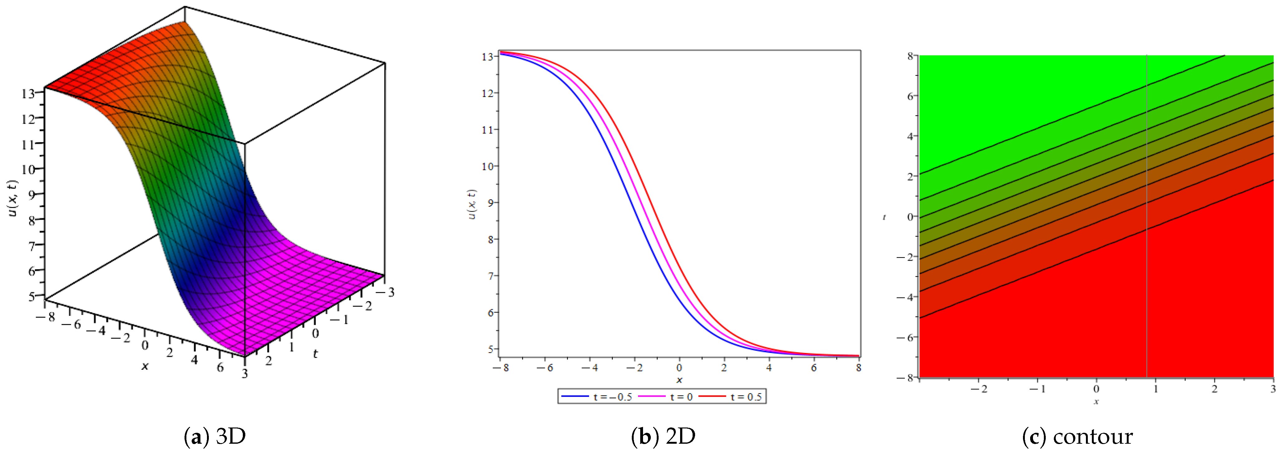
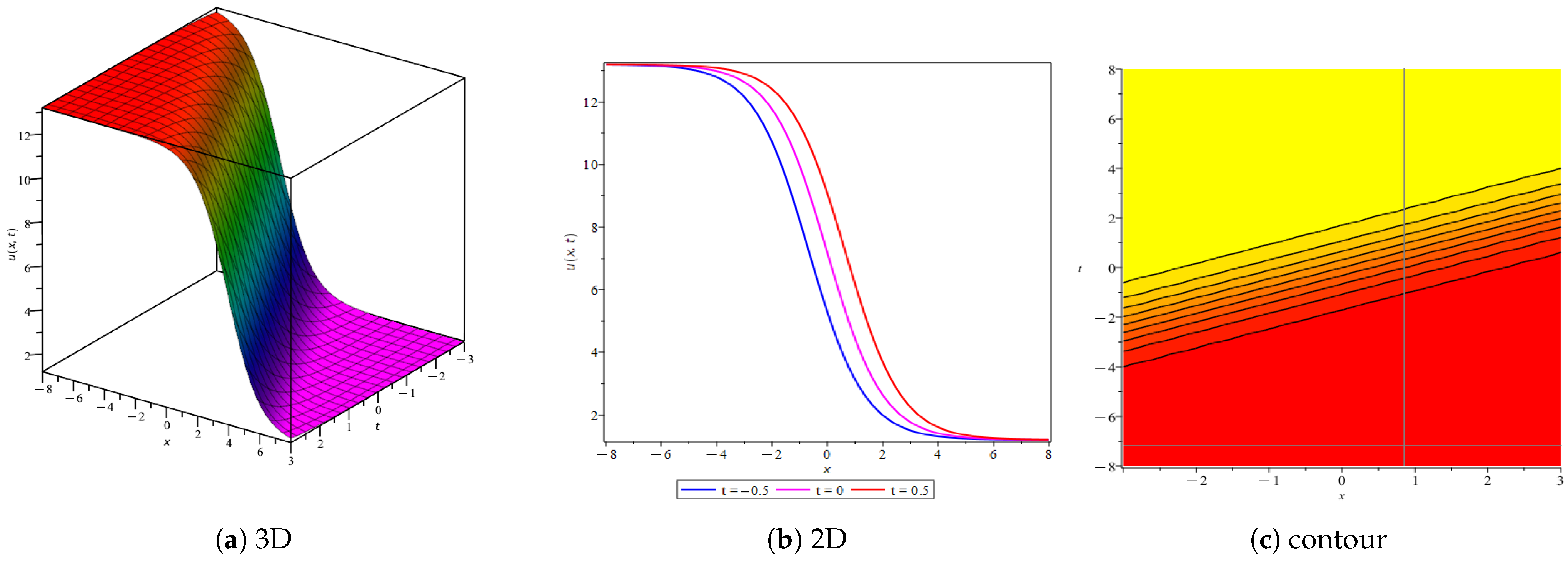
In this segment, specific values of the physical parameters are chosen to underscore the importance of the recently formulated optical solutions within the framework of the (3+1)-dimensional Boussinesq-type equation. The influence of all variables x and t on the resulting soliton solutions is illustrated through 3D, 2D, and contour graphical representations. Figure 1, Figure 2 and Figure 3 provide 3D, 2D, and contour plots that elucidate the characteristics of the solutions derived in this study. The 3D, 2D, and contour representation, the impact of temporal variables in the two-dimensional portrayal of the kink-type soliton solutions u1(x,y,z,t), is obtained via the exp-expansion method as demonstrated in Figure 1. By applying the suitable values for parameters of $u_1(x,y,z,t)$: a = 1, b = 3, E = 0.5, $\lambda =1$, $ϵ=0.4$, $\sigma =1$, $\mu =0.25$, $\nu =-1.5$, $\kappa =1$, $\tau =1$, y = 1, z = 0.5, which shows the kink soliton solutions. This is a localized and smooth change between two distinct constant states of the system at spatial infinity. Data transmission may be made more robust in less-developed systems, including optical fiber systems, by modulating input pulses to resemble the profile of kink-type solitons. In order to achieve the best possible characteristics and equivalent stress, engineers may play around with factors such as pulse width, amplitude, and fiber nonlinearity. The 3D and 2D, and the influence of the temporal parameter on the contour plots, of the kink soliton solution with suitable parameter values for u1(x,y,z,t) as derived using the Kudryashov technique are displayed in Figure 2, a = 1, b = 3, E = 0.5, $\lambda =1$, $ϵ=0.4$, $\sigma =1$, $\mu =0.25$, $\nu =-1.5$, $\kappa =1$, $\tau =1$, y = 1, z = 0.5.

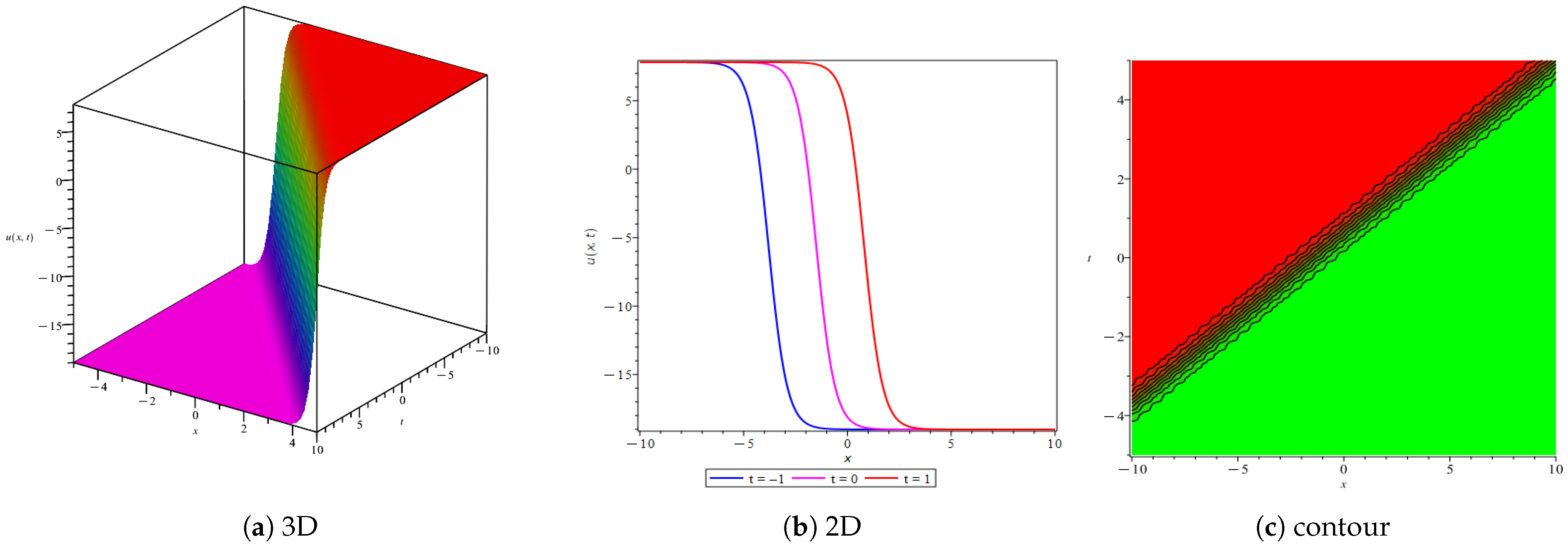
Figure 3 depicts the 3D plot, the 2D and the effect of the temporal parameter on the contour plot of the anti-kink soliton solution of the Riccati equation method of solution $u_1(x,y,z,t)$, by using the suitable values of parameters a = 1, b = 3, E = 0.5, $\lambda =1$, $ϵ=0.4$, $\sigma =1$, $\mu =0.25$, $\nu =-1.5$, $\kappa =1$, $\tau =1$, y = 1, z = 0.5. It shows the behavior of anti-kink soliton solutions. An anti-kink soliton is essentially the mirror image or opposite of a kink soliton. A kink soliton represents a smooth transition from a lower state to a higher state. An anti-kink soliton describes a smooth transition from the higher state back to the lower state.

5. Stability Analysis

This part considers stability characteristics of Equation (2). In order to determine the steady-state solutions, the function U(x) is postulated to be constant in accordance with the methodology followed in [37], leading to the assignment

$$u_{tt}-u_{xxxx}+u_{xx}+u_{xt}+u_{xy}+u_{xz}+u_x{u}_{xx}=0$$

(36)

5.1. Identify Linear and Nonlinear Terms

The PDE contains:

• Linear terms: $u_{tt},-u_{xxxx},u_{xx},u_{xt},u_{xy},u_{xz}$;
• Nonlinear term: $u_x{u}_{xx}$.

For linear stability analysis, we neglect the nonlinear term.

5.2. Linearization

Assume a small perturbation:

$$u(x,y,z,t)=ϵv(x,y,z,t),ϵ\ll 1$$

(37)

Then the nonlinear term $u_x{u}_{xx}\sim \mathcal{O}\left({ϵ}^2\right)$ can be neglected, giving the linearized PDE:

$$v_{tt}-v_{xxxx}+v_{xx}+v_{xt}+v_{xy}+v_{xz}=0$$

(38)

5.3. Fourier Mode Solution

We assume a solution of the form:

$$v(x,y,z,t)=A{e}^{i(k_{x}x+k_{y}y+k_{z}z-\omega t)}$$

(39)

where A is the amplitude, $k_x,k_y,k_z$ are wave numbers, and $\omega$ is the angular frequency.

5.4. Compute Derivatives

Using the Fourier solution, the derivatives are

$$\begin{array}{cccc}\hfill v_t& =-i\omega v,\hfill & \hfill v_{tt}& =-{\omega }^{2}v\hfill \\ \hfill v_x& =i{k}_{x}v,\hfill & \hfill v_{xx}& =-k_x^{2}v,\hfill & \hfill v_{xxxx}& =k_x^{4}v\hfill \\ \hfill v_{xy}& =-k_x{k}_{y}v,\hfill & \hfill v_{xz}=-k_x{k}_{z}v,& v_{xt}=k_x\omega v\hfill \end{array}$$

5.5. Substitute into Linearized PDE

Substituting derivatives into the linearized PDE,

$$\begin{array}{cc}\hfill v_{tt}-v_{xxxx}+v_{xx}+v_{xt}+v_{xy}+v_{xz}& =0\hfill \\ \hfill -{\omega }^{2}v-k_x^{4}v-k_x^{2}v+k_x\omega v-k_x{k}_{y}v-k_x{k}_{z}v& =0\hfill \end{array}$$

Dividing by v gives the dispersion relation

$$-{\omega }^2+k_x\omega -k_x^4-k_x^2-k_x(k_y+k_z)=0$$

(40)

5.6. Solve for $\omega$

This is a quadratic equation in $\omega$:

$${\omega }^2-k_x\omega +k_x^4+k_x^2+k_x(k_y+k_z)=0$$

(41)

The solution is

$$\omega ={\displaystyle \frac{k_x\pm \sqrt{k_x^2-4\left(k_x^4+k_x^2+k_x(k_y+k_z)\right)}}{2}}$$

(42)

5.7. Stability Condition

The solution is stable if $\omega$ is real, which requires the discriminant D to satisfy

$$\begin{array}{c}\hfill \begin{array}{c}D=k_x^2-4(k_x^4+k_x^2+k_x(k_y+k_z))\ge 0\\ \Rightarrow -4k_x^4-3k_x^2-4k_x(k_y+k_z)\ge 0\\ \Rightarrow 4k_x^4+3k_x^2+4k_x(k_y+k_z)\le 0\end{array}\end{array}$$

(43)

1. The steady state is a stable one if all the characteristic roots have negative real parts:

$$4k_x^4+3k_x^2+4k_x(k_y+k_z)>0$$

(44)

2. The steady state is of an unstable regime if at least one characteristic root has a positive real part:

$$4k_x^4+3k_x^2+4k_x(k_y+k_z)<0$$

(45)

3. or the system to be marginally unstable, the following condition must be satisfied:

$$4k_x^4+3k_x^2+4k_x(k_y+k_z)=0$$

(46)

6. Sensitivity Analysis

Sensitivity analysis constitutes a fundamental component in the identification of pivotal parameters within a system, thereby ensuring the robustness and reliability of models. This analytical approach facilitates the quantification of uncertainties, the optimization of resource allocation, and the enhancement of decision-making processes. Consider $W=U^{\prime }$ and $W^{″}=U^{‴}$. Then, Equation (17) becomes

$$2W^{″}-W^2-2\left(a_3^2+a_1+a_2-a_3+1\right)W=0.$$

(47)

Utilizing the Galilean transformation, the dynamical planar system described by Equation (47) can be reformulated as [38]

$$\left\{\begin{array}{cc}\hfill & W^{\prime }=Q,\hfill \\ \hfill & Q^{\prime }=0.5W^2+\left(a_3^2+a_1+a_2-a_3+1\right)W.\hfill \end{array}\right.$$

(48)

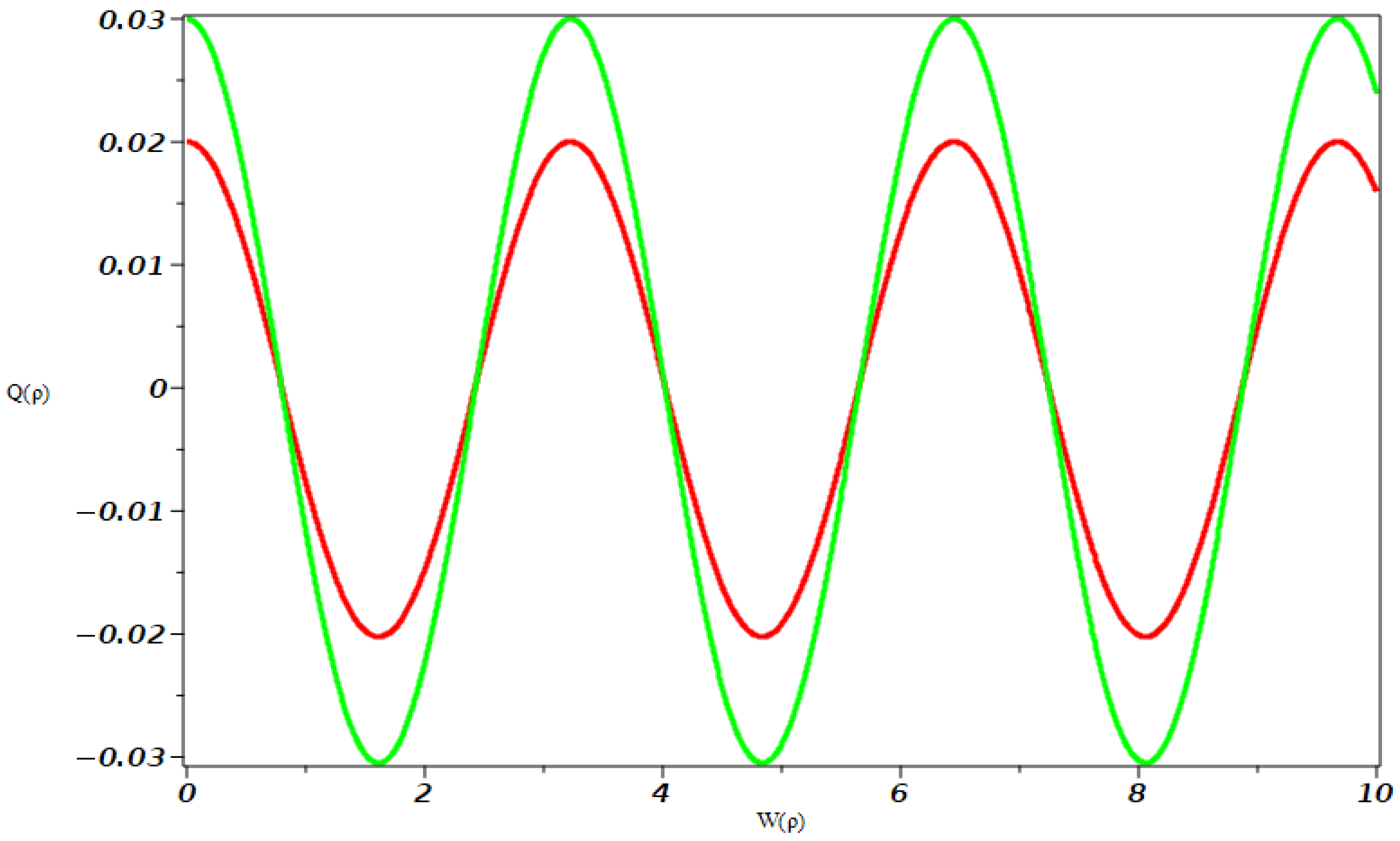
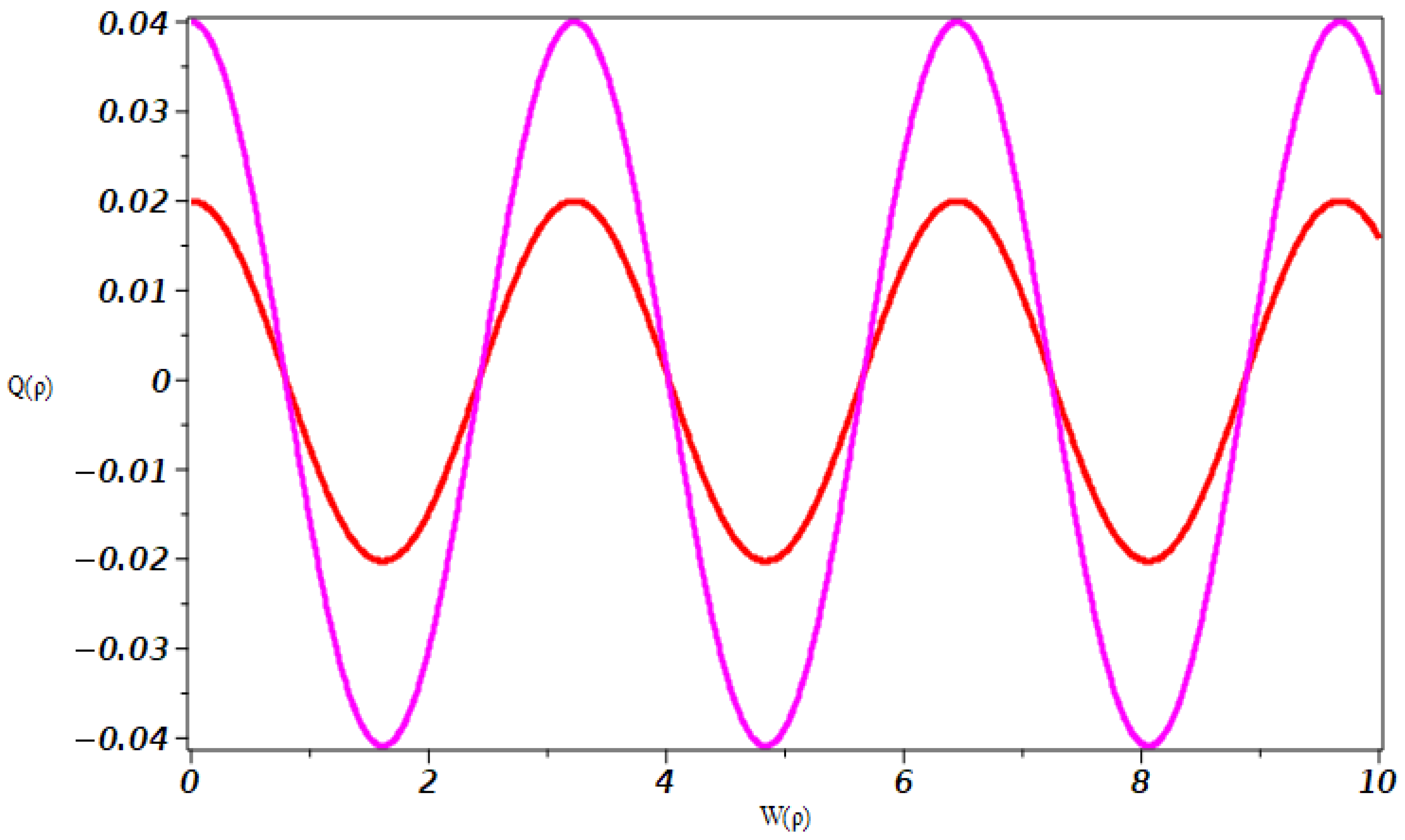
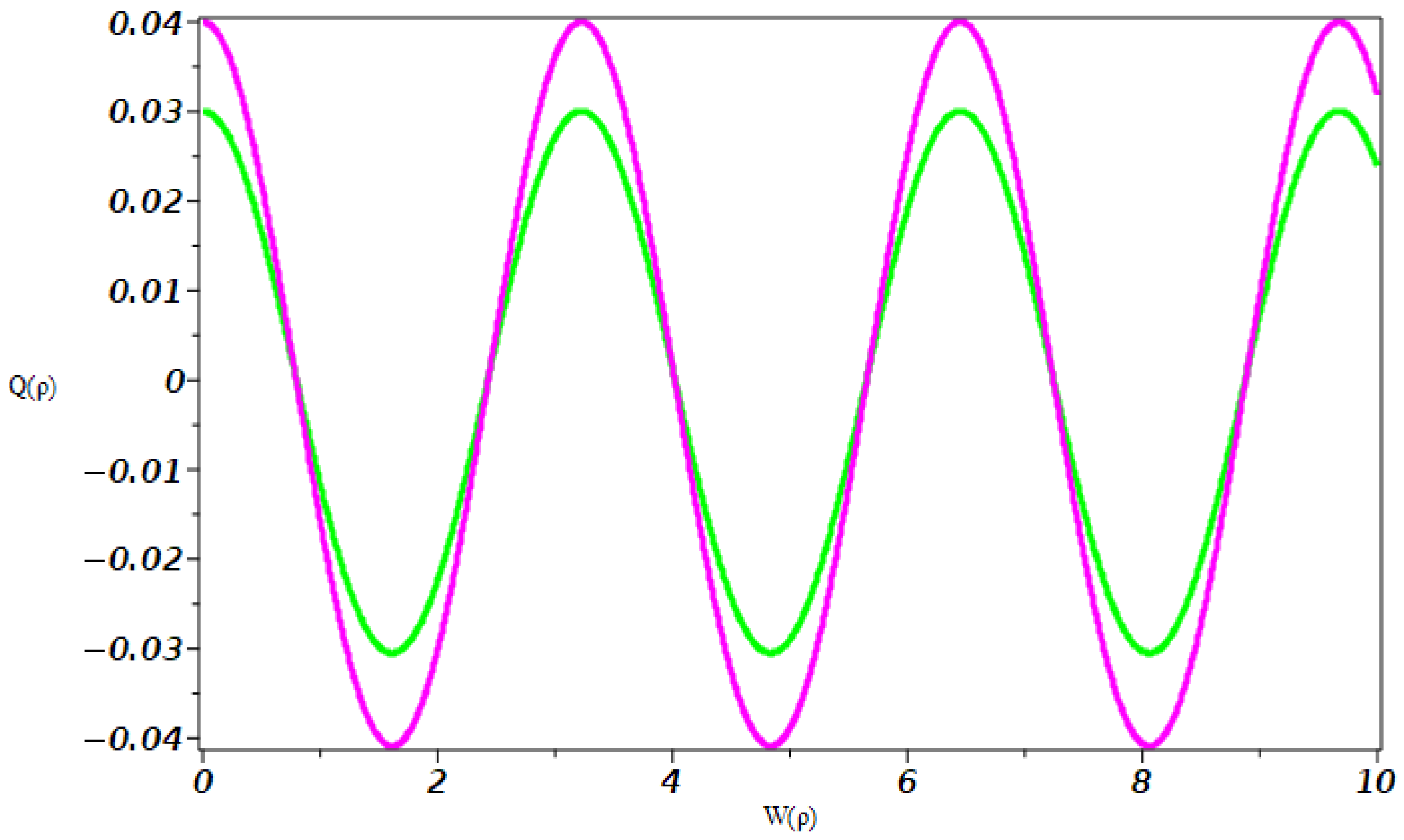
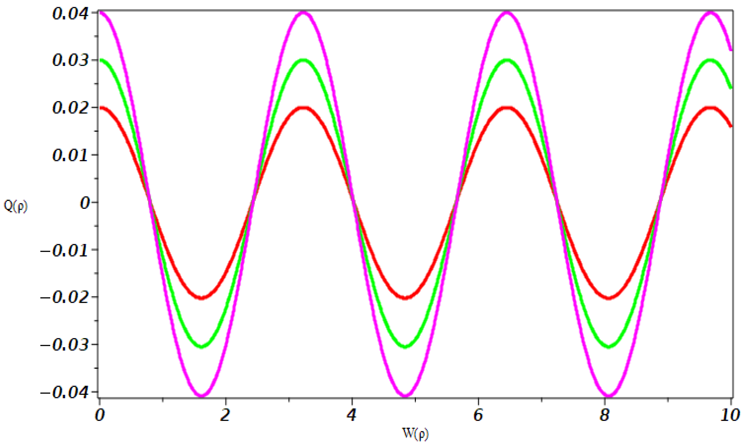
In Figure 4, Figure 5, Figure 6 and Figure 7, we analyze the system’s sensitivity using different initial conditions and fixed parameters. The graphs exhibit periodic behavior, with curves showing sensitivity to initial conditions, causing amplitude variations. Solitary waves are marked by localized pulses and stable, non-spreading wave packets. The applications of sensitivity analysis are extensive and encompass numerous domains, such as the optimization of engineering designs, the assessment of environmental impacts, and the management of financial risks. In the medical field [39], it plays a significant role in the advancement of drug development and in elucidating treatment variability, whereas in energy systems, it serves to augment the efficiency of renewable energy sources.

7. Conclusions

In this work, we explore the (3+1)-dimensional Boussinesq-type equation, which is a central nonlinear evolution equation that is used to model an extensive range of nonlinear phenomena in a variety of other scientific subjects. We derive several novel traveling wave solutions, such as rational, triangular, implicit analytic, kink, anti-kink, etc., connected to Exp-expansion, the Kudryashov method, and the Ricciati method as presented in Equations (21)–(35). These results make further contributions to the understanding of mathematical physics and pave the way for further discovery of the existence of more exact solutions. Furthermore, a Galilean transformation is applied to the resulting ordinary differential equation, and a dynamical system is obtained, allowing a sensitivity analysis to be performed under different initial conditions as in Figure 4, Figure 5 and Figure 6. This is an analysis that shows high sensitivity within the system. The implications of these findings are far-reaching into the domains of fluid dynamics, nonlinear optics, plasma physics, and geophysics, where wave propagation, energy transfer, and dynamic instabilities play an important role. The exact solutions and sensitivity knowledge displayed here could be used as useful reference marks for numerical simulations and additional theoretical studies in applied mathematical physics. Future work might involve bifurcation and chaos studies and Lie symmetries and conservation laws studies. Additionally, a range of numerical and analytical methods can be used to discover additional solutions to the problem and to gain deeper insights into the underlying dynamics of the system.

References

1. Farooq, K.; Hussain, E.; Younas, U.; Mukalazi, H.; Khalaf, T.M.; Mutlib, A.; Shah, S.A.A. Exploring the wave’s structures to the nonlinear coupled system arising in surface geometry. Sci. Rep. 2025, 15, 11624. [Google Scholar] [CrossRef] [PubMed]
2. Ismael, H.F.; Sulaiman, T.A.; Younas, U.; Nabi, H.R. On the autonomous multiple wave solutions and hybrid phenomena to a (3+1)-dimensional Boussinesq-type equation in fluid mediums. Chaos Solitons Fractals 2024, 187, 115374. [Google Scholar] [CrossRef]
3. San, S.; Beenish; Alshammari, F.S. Analytical and Dynamical Study of Solitary Waves in a Fractional Magneto-Electro-Elastic System. Fractal Fract. 2025, 9, 309. [Google Scholar] [CrossRef]
4. Billings, S.A. Nonlinear System Identification: NARMAX Methods in the Time, Frequency, and Spatio-Temporal Domains; John Wiley & Sons: Hoboken, NJ, USA, 2013. [Google Scholar] [CrossRef]
5. Gintautas, V.; Hübler, A.W. Resonant forcing of nonlinear systems of differential equations. Chaos Interdiscip. J. Nonlinear Sci. 2008, 18, 033118. [Google Scholar] [CrossRef]
6. Samreen, M.; Beenish. Bifurcation, Multistability, and Soliton Dynamics in the Stochastic Potential Korteweg-de Vries Equation. Int. J. Theor. Phys. 2025, 64, 131. [Google Scholar] [CrossRef]
7. Niwas, M.; Kumar, S.; Rajput, R.; Chadha, D. Exploring localized waves and different dynamics of solitons in (2+1)-dimensional Hirota bilinear equation: A multivariate generalized exponential rational integral function approach. Nonlinear Dyn. 2024, 112, 9431–9444. [Google Scholar] [CrossRef]
8. El-Tantawy, S.A.; Khan, D.; Khan, W.; Khalid, M.; Alhejaili, W. A novel approximation to the fractional KdV equation using the Tantawy technique and modeling fractional electron-acoustic cnoidal waves in a nonthermal plasma. Braz. J. Phys. 2025, 55, 163. [Google Scholar] [CrossRef]
9. Wazwaz, A.M.; Alhejaili, W.; El-Tantawy, S.A. Physical multiple shock solutions to the integrability of linear structures of Burgers hierarchy. Phys. Fluids 2023, 35, 123102. [Google Scholar] [CrossRef]
10. Hammad, M.A.; Khalid, M.; Alrowaily, A.W.; Tiofack, C.G.L.; El-Tantawy, S.A. Ion-acoustic cnoidal waves in a non-Maxwellian plasma with regularized κ-distributed electrons. AIP Adv. 2023, 13, 105226. [Google Scholar] [CrossRef]
11. Muhammad, J.; Younas, U.; Hussain, E.; Ali, Q.; Sediqmal, M.; Kedzia, K.; Jan, A.Z. Solitary wave solutions and sensitivity analysis to the space-time β-fractional Pochhammer–Chree equation in elastic medium. Sci. Rep. 2024, 14, 28383. [Google Scholar] [CrossRef] [PubMed]
12. Murad, M.A.S. Formation of optical soliton wave profiles of nonlinear conformable Schrödinger equation in weakly non-local media: Kudryashov auxiliary equation method. J. Opt. 2024, 54, 3177–3190. [Google Scholar] [CrossRef]
13. Murad, M.A.S. Computational analysis of the conformable nonlinear Schrödinger equation with Kudryashov’s refractive index model and generalized non-local nonlinearity. Int. J. Geom. Methods Mod. Phys. 2025, 22, 2550014. [Google Scholar] [CrossRef]
14. Wazwaz, A.M.; Alhejaili, W.; El-Tantawy, S.A. On the Painlevé integrability and nonlinear structures to a (3+1)-dimensional Boussinesq-type equation in fluid mediums: Lumps and multiple soliton/shock solutions. Phys. Fluids 2024, 36, 031702. [Google Scholar] [CrossRef]
15. Mahmood, S.S.; Murad, M.A.S. Soliton solutions to time-fractional nonlinear Schrödinger equation with cubic-quintic-septimal in weakly nonlocal media. Phys. Lett. A 2025, 532, 130183. [Google Scholar] [CrossRef]
16. Hussain, E.; Arafat, Y.; Malik, S.; Alshammari, F.S. The (2+1)-Dimensional Chiral Nonlinear Schrödinger Equation: Extraction of Soliton Solutions and Sensitivity Analysis. Axioms 2025, 14, 422. [Google Scholar] [CrossRef]
17. Hussain, E.; Shah, S.A.A.; Rafiq, M.N.; Ragab, A.E.; Az-Zo’bi, E.A. Exact solutions and modulation instability analysis of a generalized Kundu-Eckhaus equation with extra-dispersion in optical fibers. Phys. Scr. 2024, 99, 055222. [Google Scholar] [CrossRef]
18. Wang, Y.; Lü, X. Bäcklund transformation and interaction solutions of a generalized Kadomtsev–Petviashvili equation with variable coefficients. Chin. J. Phys. 2024, 89, 37–45. [Google Scholar] [CrossRef]
19. Ejaz, H.; Zhao, L.; Syed, A.A.S.; Az-Zo’bi, E.A.; Hussien, M. Dynamics study of stability analysis, sensitivity insights and precise soliton solutions of the nonlinear (STO)-Burger equation. Opt. Quantum Electron. 2023, 55, 1274. [Google Scholar] [CrossRef]
20. Mohanty, S.K.; Kravchenko, O.V.; Deka, M.K.; Dev, A.N.; Churikov, D.V. The exact solutions of the 2+1–dimensional Kadomtsev–Petviashvili equation with variable coefficients by extended generalized G G -expansion method. J. King Saud Univ. Sci. 2023, 35, 102358. [Google Scholar] [CrossRef]
21. Attaullah; Shakeel, M.; Alaoui, M.K.; Zidan, A.M.; Shah, N.A. Closed form solutions for the generalized fifth-order KDV equation by using the modified exp-function method. J. Ocean Eng. Sci. 2022; in press. [Google Scholar] [CrossRef]
22. Jafari, H.; Tajadodi, H.; Baleanu, D. Application of a homogeneous balance method to exact solutions of nonlinear fractional evolution equations. J. Comput. Nonlinear Dyn. 2014, 9, 021019. [Google Scholar] [CrossRef]
23. Malfliet, W. The tanh method: A tool for solving certain classes of nonlinear evolution and wave equations. J. Comput. Appl. Math. 2004, 164, 529–541. [Google Scholar] [CrossRef]
24. Abdou, M.A.; Soliman, A.A. Modified extended tanh-function method and its application on nonlinear physical equations. Phys. Lett. A 2006, 353, 487–492. [Google Scholar] [CrossRef]
25. Günay, B.; Kuo, C.; Ma, W.X. An application of the exponential rational function method to exact solutions to the Drinfeld–Sokolov system. Results Phys. 2021, 29, 104733. [Google Scholar] [CrossRef]
26. Beenish; Hussain, E.; Younas, U.; Tapdigoglu, R.; Garayev, M. Exploring Bifurcation, Quasi-Periodic Patterns, and Wave Dynamics in an Extended Calogero-Bogoyavlenskii-Schiff Model with Sensitivity Analysis. Int. J. Theor. Phys. 2025, 64, 146. [Google Scholar] [CrossRef]
27. Gao, X.Y. In an Ocean or a River: Bilinear Auto-Bäcklund Transformations and Similarity Reductions on an Extended Time-Dependent (3+1)-Dimensional Shallow Water Wave Equation. China Ocean Eng. 2025, 39, 160–165. [Google Scholar] [CrossRef]
28. Adel, M.; Baleanu, D.; Sadiya, U.; Arefin, M.A.; Uddin, M.H.; Elamin, M.A.; Osman, M.S. Inelastic soliton wave solutions with different geometrical structures to fractional order nonlinear evolution equations. Results Phys. 2022, 38, 105661. [Google Scholar] [CrossRef]
29. Boussinesq, J. Essai sur la Théorie des Eaux Courantes; Imprimerie Nationale: Paris, France, 1877. [Google Scholar]
30. Sui, X.; Bai, L.; Chen, Q.; Gu, G. Influencing factors of microscanning performance based on flat optical component. Chin. Opt. Lett. 2011, 9, 052302. [Google Scholar] [CrossRef]
31. Fei, R.; Wan, Y.; Hu, B.; Li, A.; Cui, Y.; Peng, H. Deep core node information embedding on networks with missing edges for community detection. Inf. Sci. 2025, 707, 122039. [Google Scholar] [CrossRef]
32. Feng, C.; Tian, B.; Yang, D.; Gao, X. Lump and hybrid solutions for a (3+1)-dimensional Boussinesq-type equation for the gravity waves over a water surface. Chin. J. Phys. 2023, 83, 515–526. [Google Scholar] [CrossRef]
33. Alekseev, G.; Brizitskii, R. Theoretical analysis of boundary value problems for generalized Boussinesq model of mass transfer with variable coefficients. Symmetry 2022, 14, 2580. [Google Scholar] [CrossRef]
34. Ershkov, S.; Burmasheva, N.; Leshchenko, D.D.; Prosviryakov, E.Y. Exact solutions of the Oberbeck–Boussinesq equations for the description of shear thermal diffusion of Newtonian fluid flows. Symmetry 2023, 15, 1730. [Google Scholar] [CrossRef]
35. Boldrini, J.L.; Fernández-Cara, E.; Rojas-Medar, M.A. An optimal control problem for a generalized Boussinesq model: The time dependent case. Rev. Mat. Complut. 2007, 20, 339–366. [Google Scholar] [CrossRef]
36. Lorca, S.A.; Boldrini, J.L. The initial value problem for a generalized Boussinesq model. Nonlinear Anal. Theory Methods Appl. 1999, 36, 457–480. [Google Scholar] [CrossRef]
37. Ahmad, S.; Mahmoud, E.E.; Saifullah, S.; Ullah, A.; Ahmad, S.; Akgül, A.; El Din, S.M. New waves solutions of a nonlinear Landau–Ginzburg–Higgs equation: The Sardar-subequation and energy balance approaches. Results Phys. 2023, 51, 106736. [Google Scholar] [CrossRef]
38. Li, Z.; Jiang, Y. Bifurcation, chaotic behavior, and traveling wave solutions for the fractional (4+1)-dimensional Davey–Stewartson–Kadomtsev–Petviashvili model. Open Phys. 2025, 23, 20250157. [Google Scholar] [CrossRef]
39. Zhao, S.; Li, Z. Bifurcation, chaotic behavior, and traveling wave solutions of the space–time fractional Zakharov–Kuznetsov–Benjamin–Bona–Mahony equation. Front. Phys. 2025, 13, 1502570. [Google Scholar] [CrossRef]
Figure 1. 3D, 2D, and contour plot of Equation (21) of exp-method by using the variables u 1 ( x , y , z , t ) : a = 1, b = 3, E = 0.5, λ = 1 , ϵ = 0.4 , σ = 1 , μ = 0.25 , ν = 1.5 , κ = 1 , τ = 1 , y = 1, z = 0.5.
Axioms 15 00198 g001
Figure 2. 3D, 2D, and contour plot of Equation (28) by selecting the suitable variables u 1 ( x , y , z , t ) : a = 1, b = 3, E = 0.5, λ = 1 , ϵ = 0.4 , σ = 1 , μ = 0.25 , ν = 1.5 , κ = 1 , τ = 1 , y = 1, z = 0.5.
Axioms 15 00198 g002
Figure 3. 3D, 2D, and contour plot of Equation (35) by choosing the perfect values of variables u 1 ( x , y , z , t ) : a = 1, b = 3, E = 0.5, λ = 1 , ϵ = 0.4 , σ = 1 , μ = 0.25 , ν = 1.5 , κ = 1 , τ = 1 , y = 1, z = 0.5.
Axioms 15 00198 g003
Figure 4. Sensitivity analysis for system (48) with parameter sets (0.02, 0) and (0.03, 0), using fixed constants: a 1 ,   b 1 , and a 3 equal to 0.40.
Axioms 15 00198 g004
Figure 5. Sensitivity analysis of system (48) using parameters (0.02, 0) and (0.04, 0) with fixed values: a 1 = 0.67 ,   b 1 = 0.45 , and a 3 = 0.40 .
Axioms 15 00198 g005
Figure 6. Sensitivity analysis of system (48) using parameters (0.03, 0) and (0.04, 0) with fixed values: a 1 = 0.67 ,   b 1 = 0.45 , and a 3 = 0.40 .
Axioms 15 00198 g006
Figure 7. Sensitivity analysis of system (48) using parameters (0.02, 0), (0.03, 0), and (0.04, 0), with fixed values: a 1 = 0.67 ,   b 1 = 0.45 , and a 3 = 0.40 .
Axioms 15 00198 g007
Disclaimer/Publisher’s Note: The statements, opinions and data contained in all publications are solely those of the individual author(s) and contributor(s) and not of MDPI and/or the editor(s). MDPI and/or the editor(s) disclaim responsibility for any injury to people or property resulting from any ideas, methods, instructions or products referred to in the content.