On the Number of Spanning Trees of New Graph Families Created from the Star Graph and the Examination of Their Entropies

Abstract

Complexity (number of spanning trees) is an essential and significant component in the design of communication networks (graphs). To ensure strong resistance and stiffness and to enhance the probability of a connection between two vertices, improvements to a network’s quality and perfection increase the number of trees that span it. Using block matrices and linear algebra techniques, we derive explicit formulas for the number of spanning trees of new graph families that are produced from star graphs in this study. The number of spanning trees in a graph is measured by the entropy of spanning trees, also known as asymptotic complexity, a graph theory metric that assesses the network’s structural robustness and dependability. Increased flexibility, stronger diverse connections, and improved resistance to random structural changes are all indicated by higher entropy. We also investigate the entropy of spanning trees on our graphs at the end of this study. Lastly, we compare the entropy of our graphs to that of other previously studied graphs with average degrees of four and five.

1. Introduction

In fields like computer networking, telecommunications, and transportation, spanning trees are essential for establishing the bare minimum of connections required to connect every component in a network or system. This is necessary for network stability, redundancy, and efficiency. By allowing only one active path for data and offering backup paths for fault tolerance, spanning trees keep networks from experiencing loops and broadcast storms [1,2,3].

Additionally, counting the number of spanning trees is done because it helps in designing efficient routing algorithms and network infrastructure, provides a sparse subgraph that reflects graph properties, and is a fundamental problem in combinatorics and graph theory with applications in physics and engineering [4,5].

A spanning tree is a minimal subset of edges that connects every vertex in a finite connected graph $G$, or a maximal subset of edges that does not contain any cycles. The history of counting the number of spanning trees $\tau (G)$ in a graph $G$ began in 1842 when the physicist Kirchhoff [6] proposed the matrix tree theorem. This was based on the determinants of a particular matrix obtained from the Laplacian matrix, $H$, which is defined by the difference between the degree matrix $D(G)$ and adjacency matrix $A(G)$. Here, $D\left(G\right)$ is a diagonal matrix, $D(G)=dig(d_1,d_2,\dots ,d_n)$, corresponding to a graph $G$ with $n$ vertices that has a vertex degree of $d_i$ in the ith position of graph $G$, and $A\left(G\right)$ is a matrix with rows and columns labeled by graph vertices, with a $1$ or $0$ in position $(v_i,v_j)$ according to whether $v_i$ and $v_j$ are adjacent or not. That is,

$$H_{ij}=\left\{\begin{array}{c}{d}_{i } \mathrm{i}\mathrm{f} i=j\hfill \\ -1 \mathrm{i}\mathrm{f} i\ne j \mathrm{a}\mathrm{n}\mathrm{d} i \mathrm{i}\mathrm{s} \mathrm{a}\mathrm{d}\mathrm{j}\mathrm{a}\mathrm{c}\mathrm{e}\mathrm{n}\mathrm{t} \mathrm{t}\mathrm{o} j\hfill \\ 0\mathrm{o}\mathrm{t}\mathrm{h}\mathrm{e}\mathrm{r}\mathrm{w}\mathrm{i}\mathrm{s}\mathrm{e}\hfill \end{array}\right.$$

where $d_i$ denotes the degree of vertex $v_i$.

The matrix tree theorem states that all the cofactors of $H$ are equal and their common value is equal to the complexity $\tau (G)$.

For some distinctive categories of graphs, there exist simple closed formulas that make it much easier to enumerate the number of corresponding spanning trees, especially when these numbers are very large. Cayley [7] showed that a complete graph $K_n$ has $n^{n-2},n\ge 2$, spanning trees. Another result is $\tau (K_{m,n})=m^{n-1}{n}^{m-1},n,m\ge 1$, where $K_{m,n}$ is the complete bipartite graph with bipartite sets that have $m$ and $n$ vertices, respectively. This is widely recognized as in, e.g., [8]. Sedlacek [9] achieved another result by deriving a formula for the wheel on $n+1$ vertices, $W_{n+1}$. He demonstrated that, for $n\ge 3$, $\tau (W_{n+1})=({\displaystyle \frac{3+\sqrt{5}}{2}}{)}^n+({\displaystyle \frac{3-\sqrt{5}}{2}}{)}^n-2$.

Additionally, Sedlacek [10] later deduced a formula for the number of spanning trees in a Mobius ladder $M_n: \tau (M_n)={\displaystyle \frac{n}{2}}[(2+\sqrt{3}{)}^n+(2-\sqrt{3}{)}^n+2]$ for $n\ge 2$.

Moreover, Boesch and Bogdanowicz [11] utilized the matrix tree theorem to derive the number of spanning trees for a prism graph $R_n$ with $2n$ vertices:$\tau (P_n)={\displaystyle \frac{1}{2}}[(2+\sqrt{3}{)}^n+(2-\sqrt{3}{)}^n]-1]$ for $n\ge 3.$

Numerous closed formulas for determining and optimizing the number of spanning trees for specific graph families have recently been published using the matrix tree theorem [12,13,14].

There is an additional way to calculate $\tau (G)$. Assume that ${\mu }_1\ge {\mu }_2\ge \dots \ge {\mu }_k=0$ represent the eigenvalues of the matrix $H$ of a graph $G$, which has $n$ vertices. “Chelnokov” and “Kelmans” [15] have deduced that

$$\tau (G)={\displaystyle \frac{1}{k}}{\prod }_{i=1}^{k-1}{\mu }_k.$$

(1)

A popular technique for determining complexity is the deletion–contraction method. When $e$ is any edge in a graph $G$, its complexity $\tau (G)$ is equal to $\tau (G)=\tau (G-e)+\tau (G/e)$, where $G-e$ is the deletion of $e$ and $G/e$ is the contraction of $e$ in $G$. In this way, the complexity of a graph can be determined recursively [16,17].

There is also another iterative method for calculating the number of spanning trees, which is to simplify the graph and observe the changes in the number of weighted spanning trees. The electrically equivalent transformation method applies graph transformations, such as combining serial edges, merging parallel edges, and converting between triangle (Δ) and star (Y) configurations, by utilizing the connection between electrical networks—where conductance is represented by edge weights—and the counting spanning tree problem. By applying the theory of electrical networks, Yilun Shang [18] obtained a closed-form formula for the enumeration of spanning trees in the subdivided-line graph of a simple connected graph.

Recently, Asiri and Daoud [19,20] derived some explicit formulas for certain pyramid graphs based on some nonahedral graphs and Fritsch graphs using this method.

2. Some Properties of Chebyshev Polynomials

In this subsection we give certain numerous properties of Chebyshev polynomials which play an important role in our computations, from Boesch [21,22]. The Chebyshev polynomial of the first kind, $T_n(x)$, is defined as

$$T_n(\mathit{cos}x)=\mathit{cos}(nx)$$

(2)

or equivalently

$$T_n(x)=\mathit{cos}(n{\mathit{cos}}^{-1}x)$$

(3)

since

$T_0(x)=\mathit{cos}(0{\mathit{cos}}^{-1}x)=1,T_1(x)=\mathit{cos}(1{\mathit{cos}}^{-1}x)=x,T_2(x)=\mathit{cos}(2{\mathit{cos}}^{-1}x)=2x^2-1,T_3(x)=\mathit{cos}(3{\mathit{cos}}^{-1}x)=4x^3-3x,T_4(x)=\mathit{cos}(4{\mathit{cos}}^{-1}x)=8x^4-8x^2+1,\mathrm{and} \mathrm{so} \mathrm{on}.$

We can define $T_n(x)$ if we assume $x=cos\theta$ in the form

$$\begin{array}{cc}\hfill T_n\left(x\right)& =\mathit{cos}(n\theta )\hfill \\ & ={\displaystyle \frac{1}{2}}[e^{in\theta }+e^{-in\theta }]\hfill \\ & ={\displaystyle \frac{1}{2}}[{(cos\theta +isin\theta )}^n+{(cos\theta -isin\theta )}^n]\hfill \\ & ={\displaystyle \frac{1}{2}}[(x+i\sqrt{1-x^2}{)}^n+(x-i\sqrt{1-x^2}{)}^n]\hfill \\ & ={\displaystyle \frac{1}{2}}[(x+\sqrt{x^2-1}{)}^n+(x-\sqrt{x^2-1}{)}^n]\hfill \end{array}$$

(4)

The Chebyshev polynomial of the second kind, $U_n(x)$, is defined as

$$U_n(x)={\displaystyle \frac{1}{n+1}}{\displaystyle \frac{d}{dx}}{T}_{n+1}(x)={\displaystyle \frac{\mathit{sin}((n+1){\mathit{cos}}^{-1}x)}{\mathit{sin}({\mathit{cos}}^{-1}x)}}$$

(5)

Thus, we conclude that

$$U_n(x)={\displaystyle \frac{1}{2\sqrt{x^2-1}}}[(x+\sqrt{x^2-1}{)}^{n+1}-(x-\sqrt{x^2-1}{)}^{n+1}]$$

(6)

Since $U_{n-1}(\mathit{cos}{\displaystyle \frac{k\pi }{n}})=\mathrm{0,1}\le k\le n-1$, we obtain

$$U_{n-1}(x)=2^{n-1}{\prod }_{k=1}^{n-1}(x-\mathit{cos}{\displaystyle \frac{k\pi }{n}})$$

(7)

Additionally, one observes that

$$U_{n-1}(-x)=2^{n-1}{\prod }_{k=1}^{n-1}(x+\mathit{cos}{\displaystyle \frac{k\pi }{n}})$$

(8)

From identities (7) and (8), we get

$${U_{n-1}}^2(x)=4^{n-1}{\prod }_{k=1}^{n-1}(x^2-{\mathit{cos}}^2{\displaystyle \frac{k\pi }{n}}),$$

(9)

Therefore,

$$U_{n-1}^2(\sqrt{{\displaystyle \frac{x+2}{4}}})={\prod }_{k=1}^{n-1}(x-2\mathit{cos}{\displaystyle \frac{2k\pi }{n}})$$

(10)

Also, we can see that

$${\prod }_{k=1}^{n-1}(2-2\mathit{cos}{\displaystyle \frac{k\pi }{n}})=n,n\ge 2$$

(11)

$${\prod }_{k=1}^{n-1}(2-2\mathit{cos}{\displaystyle \frac{2k\pi }{n}})=n^2,n\ge 2$$

(12)

Polynomials $T_n(x)$ and $U_{n-1}(x)$ are joined by the next identity

$$U_{n-1}^2(x)={\displaystyle \frac{T_n(2x^2-1)-1}{2(x^2-1)}}$$

(13)

Lemma 1.

([12]). Let $A_n(x)$ be an $n\times n$ circulant matrix such that

$$A_n(x)=\left(\begin{array}{cccccc}x& -1& 0& \dots & 0& -1\\ -1& \ddots & \ddots & \ddots & \ddots & 1\\ 0& \ddots & \ddots & \ddots & \ddots & ⋮\\ ⋮& \ddots & \ddots & \ddots & \ddots & 1\\ 0& \ddots & \ddots & \ddots & \ddots & -1\\ -1& 0& \dots & 0& -1& x\end{array}\right).$$

Then for $n\ge 3,x\ge 4,$ we have $\mathit{det}(A_n(x))=2[T_n({\displaystyle \frac{x}{2}})-1].$

Lemma 2.

([23]). Let $P\in F^{n\times n}$, $Q\in F^{n\times m}$, $R\in F^{m\times n}$, and $T\in F^{m\times m}$. Suppose that P and $T$ are nonsingular matrices; then $\mathit{det}\left(\begin{array}{cc}P& Q\\ R& T\end{array}\right)=\mathit{det}(P-Q{T}^{-1}R)\mathit{det}T=\mathit{det}P\mathit{det}(T-R{P}^{-1}Q).$

Lemma 3.

([23]). If $A\in F^{n\times n}$,$B\in F^{n\times m}$,$B^t\in F^{m\times n}$ , and $C\in F^{m\times m}$ , then

$$\det \left(\begin{array}{cc}\mathrm{A}& \mathrm{B}\\ {\mathrm{B}}^{\mathrm{t}}& \mathrm{C}\end{array}\right)=\det (\mathrm{A}\times \mathrm{C}-\mathrm{B}\times {\mathrm{B}}^{\mathrm{t}}),{\mathrm{B}}^{\mathrm{t}}\times \mathrm{C}=\mathrm{C}\times {\mathrm{B}}^{\mathrm{t}}.$$

Our calculations for the complexity of the graphs examined in this study are made easier by these two lemmas, which give some matrices a sort of symmetry. To aid us in our computations, we also present the following important lemma:

Lemma 4.

Let $X$ be a four-block matrix with $n\times n$ matrices. Its structure is as follows.

$$X=\left(\begin{array}{cccccccccc}a& 0& \dots & \dots & 0& 0& -1& 0& \dots & 0\\ 0& \ddots & \ddots & \ddots & ⋮& 0& \ddots & \ddots & \ddots & ⋮\\ ⋮& \ddots & \ddots & \ddots & ⋮& ⋮& \ddots & \ddots & \ddots & 0\\ ⋮& \ddots & \ddots & \ddots & 0& 0& \ddots & \ddots & \ddots & -1\\ 0& \dots & \dots & 0& a& -1& 0& \dots & 0& 0\\ 0& 0& \dots & 0& -1& b& 0& \dots & \dots & 0\\ -1& \ddots & \ddots & \ddots & 0& 0& \ddots & \ddots & \ddots & ⋮\\ 0& \ddots & \ddots & \ddots & ⋮& ⋮& \ddots & \ddots & \ddots & ⋮\\ ⋮& \ddots & \ddots & \ddots & 0& ⋮& \ddots & \ddots & \ddots & 0\\ 0& \dots & 0& -1& 0& 0& \dots & \dots & 0& b\end{array}\right).$$

Then for $ab\ne 1, detX=({ab-1)}^n,$ and

$$X^{-1}=\left(\begin{array}{cccccccccc}{\displaystyle \frac{b}{ab-1}}& 0& \dots & \dots & 0& 0& {\displaystyle \frac{1}{ab-1}}& 0& \dots & 0\\ 0& \ddots & \ddots & \ddots & ⋮& 0& \ddots & \ddots & \ddots & ⋮\\ ⋮& \ddots & \ddots & \ddots & ⋮& ⋮& \ddots & \ddots & \ddots & 0\\ ⋮& \ddots & \ddots & \ddots & 0& 0& \ddots & \ddots & \ddots & {\displaystyle \frac{1}{ab-1}}\\ 0& \dots & \dots & 0& {\displaystyle \frac{b}{ab-1}}& {\displaystyle \frac{1}{ab-1}}& 0& \dots & 0& 0\\ 0& 0& \dots & 0& {\displaystyle \frac{1}{ab-1}}& {\displaystyle \frac{a}{ab-1}}& 0& \dots & \dots & 0\\ {\displaystyle \frac{1}{ab-1}}& \ddots & \ddots & \ddots & 0& 0& \ddots & \ddots & \ddots & ⋮\\ 0& \ddots & \ddots & \ddots & ⋮& ⋮& \ddots & \ddots & \ddots & ⋮\\ ⋮& \ddots & \ddots & \ddots & 0& ⋮& \ddots & \ddots & \ddots & 0\\ 0& \dots & 0& {\displaystyle \frac{1}{ab-1}}& 0& 0& \dots & \dots & 0& {\displaystyle \frac{a}{ab-1}}\end{array}\right).$$

3. Main Results

Extracting a new structure from an existing one is always the aim in mathematics. This is also true in the realm of graphs, where many new graphs can be created from a given set of graphs. In this work, we define several new graph families created based on the star graph, $S_n$, and then we calculate the number of spanning trees for these graphs.

Counting the number of spanning trees $\tau (G)$ in graphs formed from star graphs is essential for assessing network dependability. These computations are essential for chemical isomer stability, network communication path optimization, and statistical physics (e.g., self-organized criticality in sand-pile models), because they evaluate redundancy and fault tolerance.

Definition 1.

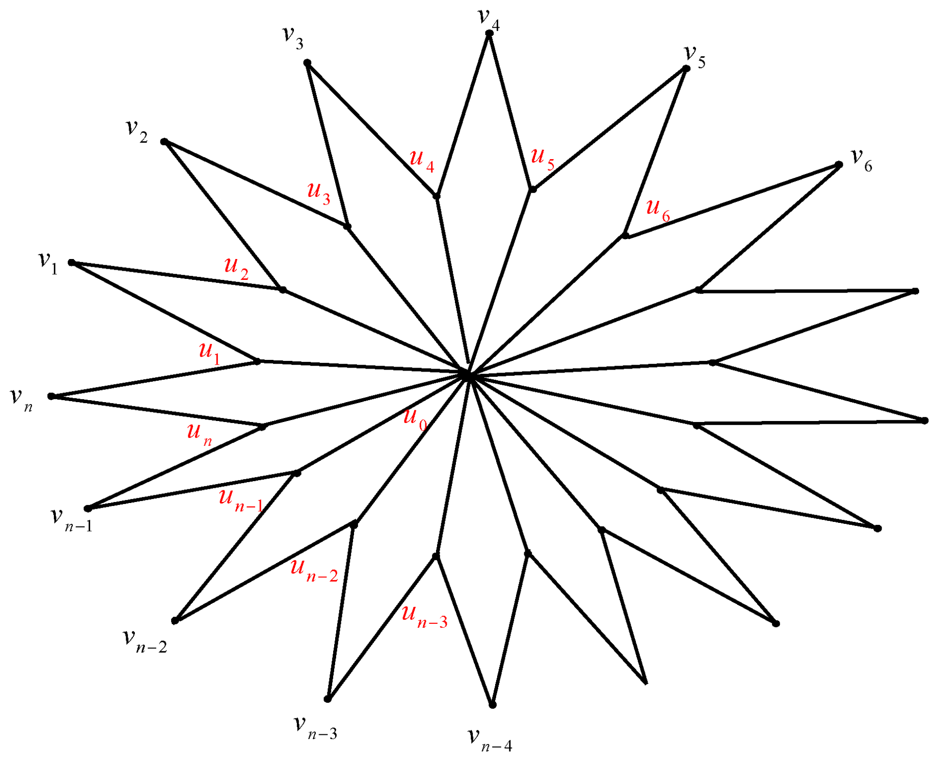
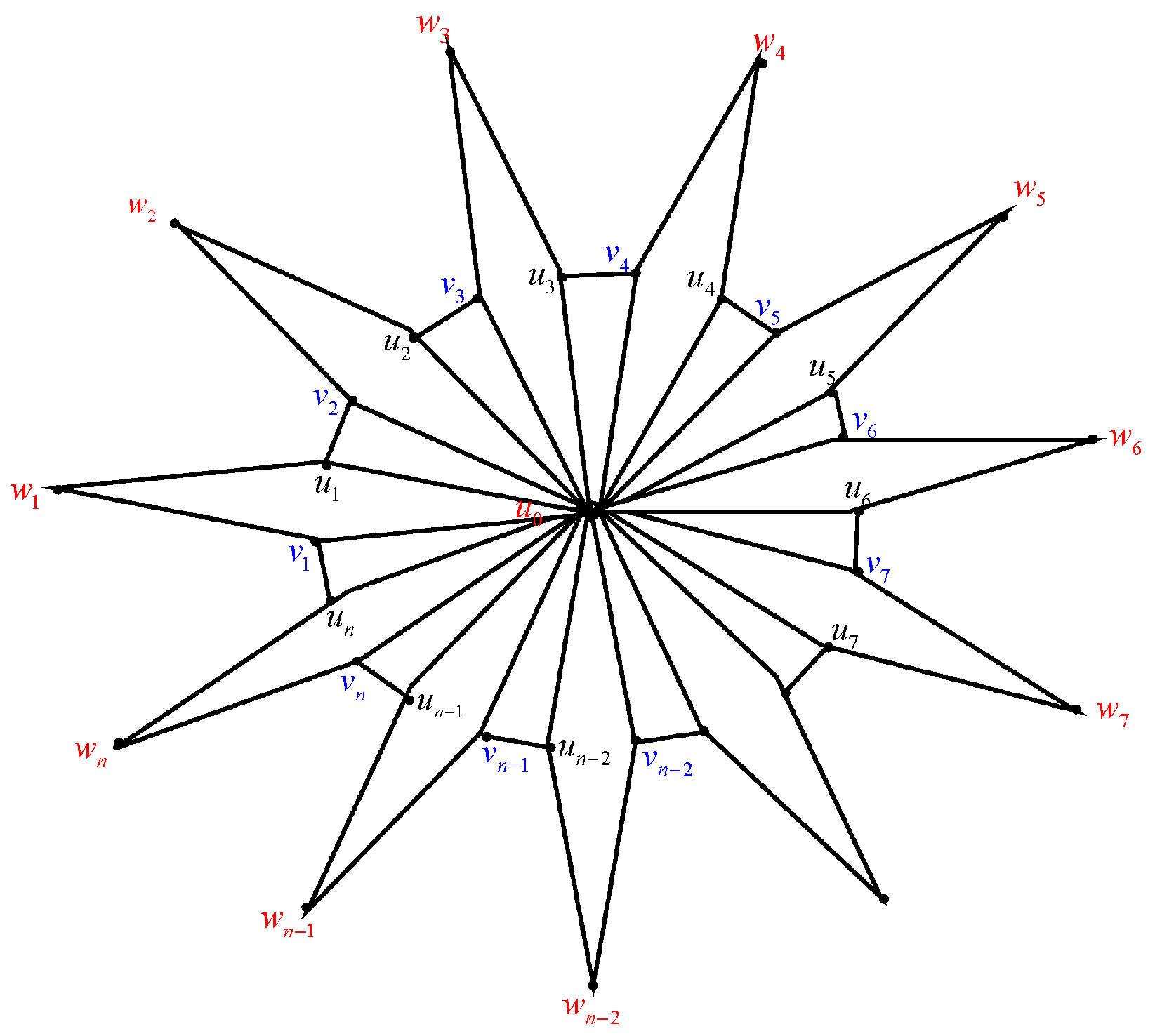
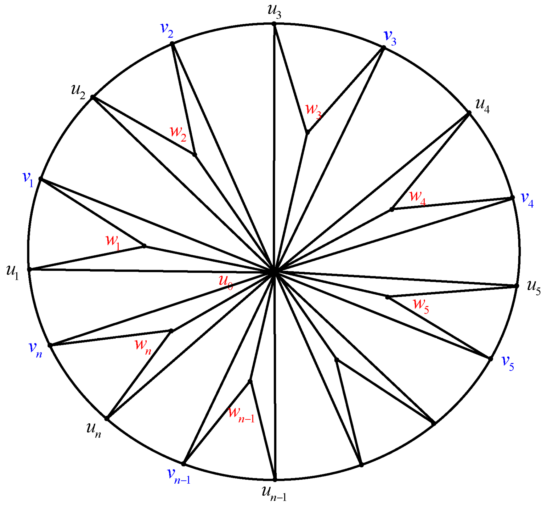
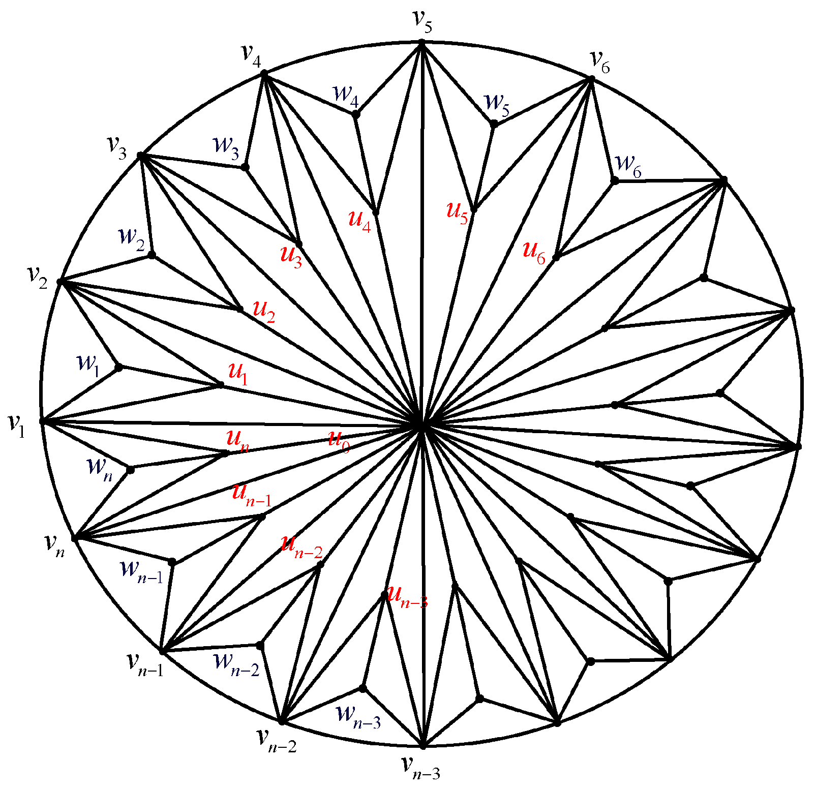
For $n\ge 3,$ the cog star graph, or $C{S}_n$, is the graph that is produced by combining the star graph $S_n=\left\{u_0,u_1,u_2,\dots ,u_n\right\}$ with a collection of vertices $\{v_1,v_2,\dots ,v_n\}$. This is done so that for $1\le i\le n-1$, vertex $v_i$ is adjacent to vertices $u_i$ and $u_{i+1}$, while vertex $v_n$ is adjacent to vertices $u_1$ and $u_n$, as illustrated in Figure 1.

Obviously, the cog star graph $C{S}_n$ has order $\left|V(C{S}_n)\right|=2n+1$ and size $\left|E(C{S}_n)\right|=3n$, and, hence, for large values of $n$, its average degree is $3$.

Theorem 1.

For $n\ge 3$, we have $\tau (C{S}_n)=(2+\sqrt{3}{)}^n+(2-\sqrt{3}{)}^n-2$.

Proof. 

From the matrix tree theorem, we have

$$\tau (C{S}_n)=\mathit{det}\left(\begin{array}{cccccccccc}3& 0& \dots & \dots & 0& -1& 0& \dots & 0& -1\\ 0& \ddots & \ddots & \ddots & ⋮& -1& \ddots & \ddots & \ddots & 0\\ ⋮& \ddots & \ddots & \ddots & ⋮& 0& \ddots & \ddots & \ddots & ⋮\\ ⋮& \ddots & \ddots & \ddots & 0& ⋮& \ddots & \ddots & \ddots & 0\\ 0& \dots & \dots & 0& 3& 0& \dots & 0& -1& -1\\ -1& -1& 0& \dots & 0& 2& 0& \dots & \dots & 0\\ 0& \ddots & \ddots & \ddots & ⋮& 0& \ddots & \ddots & \ddots & ⋮\\ ⋮& \ddots & \ddots & \ddots & 0& ⋮& \ddots & \ddots & \ddots & ⋮\\ 0& \ddots & \ddots & \ddots & -1& ⋮& \ddots & \ddots & \ddots & 0\\ -1& 0& \dots & 0& -1& 0& \dots & \dots & 0& 2\end{array}\right)=\mathit{det}\left( \begin{array}{cc}P& Q\\ R& S\end{array} \right).$$

Using Lemma (2), we obtain

$$\begin{array}{cc}\hfill \tau \left(C{S}_n\right)& =detP\times \mathrm{d}\mathrm{e}\mathrm{t}[S-R{P}^{-1}Q]\hfill \\ & =3^n\times \mathit{det}\left(\begin{array}{cccccc}{\displaystyle \frac{4}{3}}& -{\displaystyle \frac{1}{3}}& 0& \dots & 0& -{\displaystyle \frac{1}{3}}\\ -{\displaystyle \frac{1}{3}}& \ddots & \ddots & \ddots & \ddots & 0\\ 0& \ddots & \ddots & \ddots & \ddots & ⋮\\ ⋮& \ddots & \ddots & \ddots & \ddots & 0\\ 0& \ddots & \ddots & \ddots & \ddots & -{\displaystyle \frac{1}{3}}\\ -{\displaystyle \frac{1}{3}}& 0& \dots & 0& -{\displaystyle \frac{1}{3}}& {\displaystyle \frac{4}{3}}\end{array}\right)=\mathit{det}\left(\begin{array}{cccccc}4& -1& 0& \dots & 0& -1\\ -1& \ddots & \ddots & \ddots & \ddots & 0\\ 0& \ddots & \ddots & \ddots & \ddots & ⋮\\ ⋮& \ddots & \ddots & \ddots & \ddots & 0\\ 0& \ddots & \ddots & \ddots & \ddots & -1\\ -1& 0& \dots & 0& -1& 4\end{array}\right)\hfill \end{array}.$$

By applying Lemma (1), we get

$$\tau (C{S}_n)=2[T_n(2)-1].$$

The result comes from Equation (4). $\square$

Definition 2.

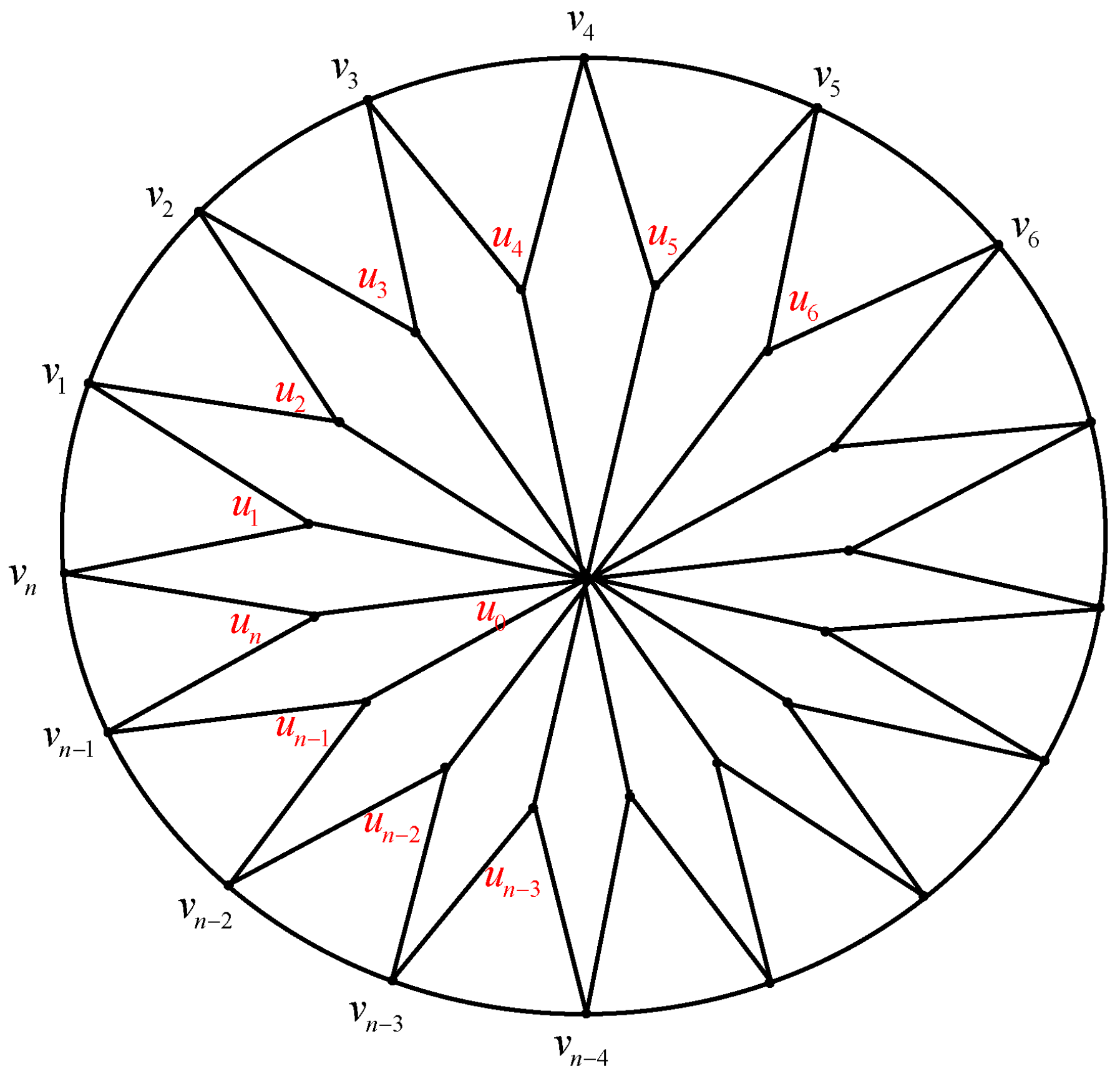
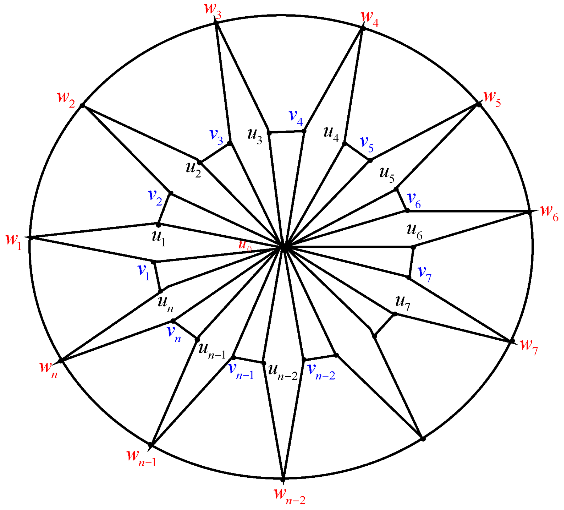
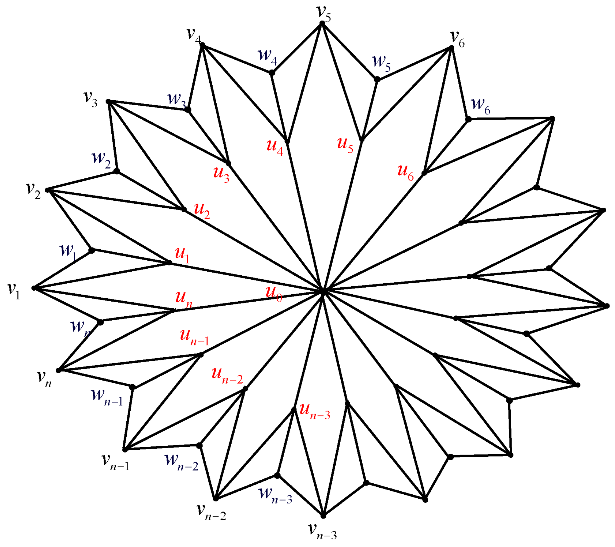
For $n\ge 3,$ the closed cog star graph, ${CCS}_n$, is a graph that is produced by the union of the cycle graph $C_n=\left\{v_1,v_2,\dots ,v_n\right\}$ and the cog star graph $C{S}_n$, as seen in Figure 2.

Obviously, the closed cog star graph $CC{S}_n$ has order $\left|V(CC{S}_n)\right|=2n+1$ and size $\left|E(CC{S}_n)\right|=4n$, and, hence, for large values of $n$, its average degree is $4$.

Theorem 2.

For $n\ge 3$, we have $\tau ({CCS}_n)=2^n[2^{2n}-2^{n+1}+1].$

Proof. 

From the matrix tree theorem, we have

$$\tau \left({CCS}_n\right)=\mathit{det}\left(\begin{array}{cccccccccccc}3& 0& \dots & \dots & \dots & 0& -1& 0& \dots & \dots & 0& -1\\ 0& \ddots & \ddots & \ddots & \ddots & ⋮& -1& \ddots & \ddots & \ddots & \ddots & 0\\ ⋮& \ddots & \ddots & \ddots & \ddots & ⋮& 0& \ddots & \ddots & \ddots & \ddots & ⋮\\ ⋮& \ddots & \ddots & \ddots & \ddots & ⋮& ⋮& \ddots & \ddots & \ddots & \ddots & ⋮\\ ⋮& \ddots & \ddots & \ddots & \ddots & 0& 0& \ddots & 0& \ddots & \ddots & 0\\ 0& \dots & \dots & \dots & 0& 3& 0& \dots & \dots & 0& -1& -1\\ -1& -1& 0& \dots & \dots & 0& 4& -1& 0& \dots & \dots & -1\\ 0& \ddots & \ddots & \ddots & \ddots & ⋮& -1& \ddots & \ddots & \ddots & \ddots & 0\\ ⋮& \ddots & \ddots & \ddots & \ddots & ⋮& 0& \ddots & \ddots & \ddots & \ddots & ⋮\\ ⋮& \ddots & \ddots & \ddots & \ddots & 0& ⋮& \ddots & \ddots & \ddots & \ddots & 0\\ 0& \ddots & \ddots & \ddots & \ddots & -1& 0& \ddots & \ddots & \ddots & \ddots & -1\\ -1& 0& \dots & \dots & 0& -1& -1& 0& \dots & 0& -1& 4\end{array}\right)=\mathit{det}\left( \begin{array}{cc}P& Q\\ R& S\end{array} \right).$$

By applying Lemma (2), we get

$$\begin{array}{cc}\hfill \tau \left(CC{S}_n\right)& =detP\times \mathrm{d}\mathrm{e}\mathrm{t}[S-R{P}^{-1}Q]\hfill \\ & =3^n\times \mathit{det}\left(\begin{array}{cccccc}{\displaystyle \frac{10}{3}}& -{\displaystyle \frac{4}{3}}& 0& \dots & 0& -{\displaystyle \frac{4}{3}}\\ -{\displaystyle \frac{4}{3}}& \ddots & \ddots & \ddots & \ddots & 0\\ 0& \ddots & \ddots & \ddots & \ddots & ⋮\\ ⋮& \ddots & \ddots & \ddots & \ddots & 0\\ 0& \ddots & \ddots & \ddots & \ddots & -{\displaystyle \frac{4}{3}}\\ -{\displaystyle \frac{4}{3}}& 0& \dots & 0& -{\displaystyle \frac{4}{3}}& {\displaystyle \frac{10}{3}}\end{array}\right)=4^n\mathit{det}\left(\begin{array}{cccccc}{\displaystyle \frac{5}{2}}& -1& 0& \dots & 0& -1\\ -1& \ddots & \ddots & \ddots & \ddots & 0\\ 0& \ddots & \ddots & \ddots & \ddots & ⋮\\ ⋮& \ddots & \ddots & \ddots & \ddots & 0\\ 0& \ddots & \ddots & \ddots & \ddots & -1\\ -1& 0& \dots & 0& -1& {\displaystyle \frac{5}{2}}\end{array}\right).\hfill \end{array}$$

Using Lemma (1), we obtain

$$\tau \left(CC{S}_n\right)=4^n\times 2[T_n({\displaystyle \frac{5}{4}})-1]$$

The result comes from Equation (4). $\square$

Definition 3.

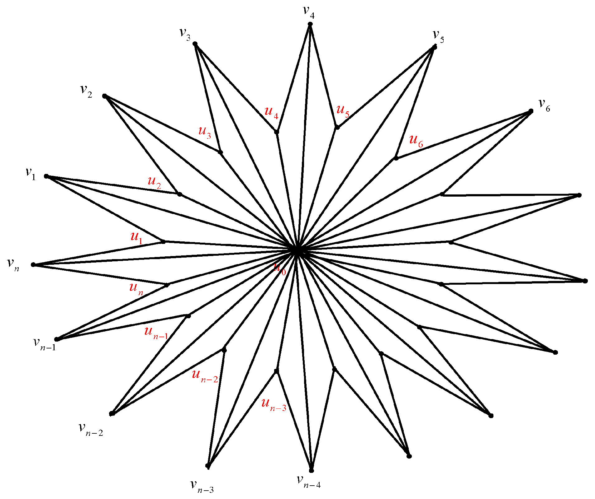
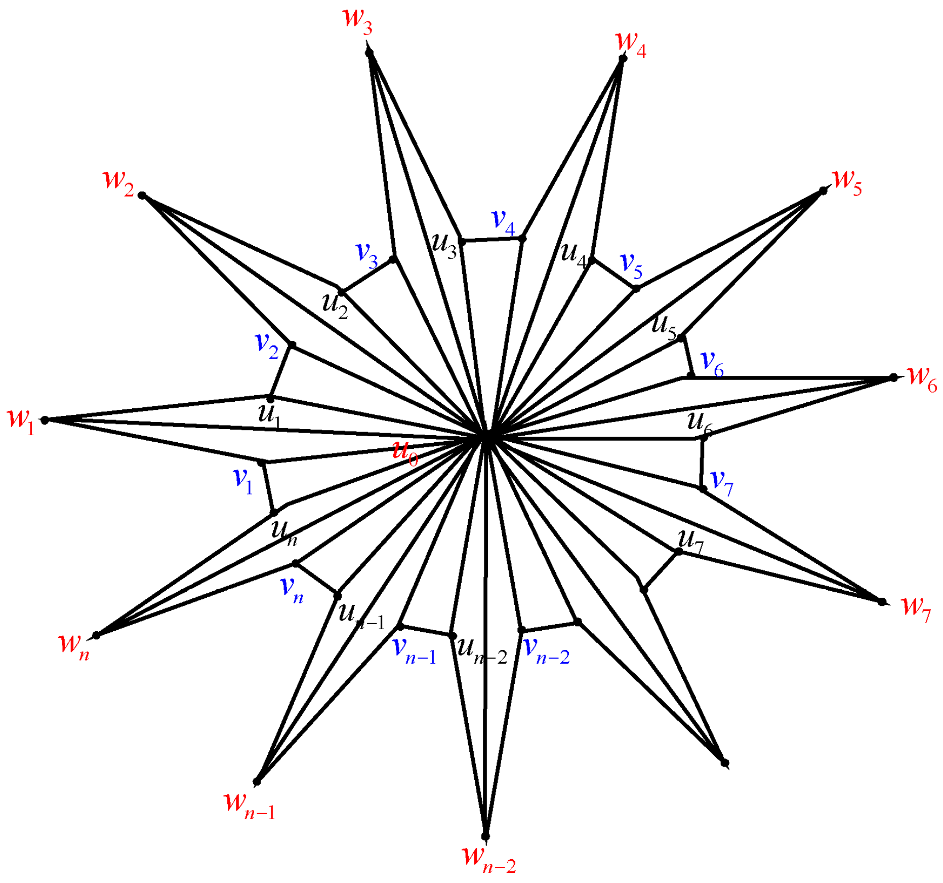
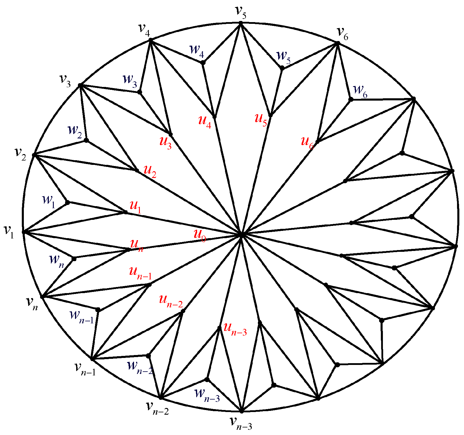
For $n\ge 3,$ the cog double-star graph, $CD{S}_n$, is the graph that is produced by combining two star graphs $S_n=\left\{u_0,u_1,u_2,\dots ,u_n\right\}$ and $S_n=\left\{u_0,v_1,v,\dots ,v_n\right\}$. This is done so that for $1\le i\le n-1$, vertex $v_i$ is adjacent to vertices $u_i$ and $u_{i+1}$, while vertex $v_n$ is adjacent to vertices $u_1$ and $u_n$, as shown in Figure 3.

Obviously, the cog double-star graph $CD{S}_n$ has order $\left|V(CD{S}_n)\right|=2n+1$ and size $\left|E(CD{S}_n)\right|=4n$, and, hence, for large values of $n$, its average degree is $4$.

Theorem 3.

For $n\ge 3$, we have $\tau (CD{S}_n)=( {\displaystyle \frac{1}{2 }}{)}^n [(7+3\sqrt{5}{)}^n+(7-3\sqrt{5}{)}^n-2^{n+1}].$

Proof. 

From the matrix tree theorem, we have

$$\tau \left(CD{S}_n\right)=\mathit{det}\left(\begin{array}{cccccccccc}3& 0& \dots & \dots & 0& -1& 0& \dots & 0& -1\\ 0& \ddots & \ddots & \ddots & ⋮& -1& \ddots & \ddots & \ddots & 0\\ ⋮& \ddots & \ddots & \ddots & ⋮& 0& \ddots & \ddots & \ddots & ⋮\\ ⋮& \ddots & \ddots & \ddots & 0& ⋮& \ddots & \ddots & \ddots & 0\\ 0& \dots & \dots & 0& 3& 0& \dots & 0& -1& -1\\ -1& -1& 0& \dots & 0& 3& 0& \dots & \dots & 0\\ 0& \ddots & \ddots & \ddots & ⋮& 0& \ddots & \ddots & \ddots & ⋮\\ ⋮& \ddots & \ddots & \ddots & 0& ⋮& \ddots & \ddots & \ddots & ⋮\\ 0& \ddots & \ddots & \ddots & -1& ⋮& \ddots & \ddots & \ddots & 0\\ -1& 0& \dots & 0& -1& 0& \dots & \dots & 0& 3\end{array}\right)=\mathit{det}\left(\begin{array}{cc}P& Q\\ R& S\end{array}\right).$$

Using Lemma (2), we obtain

$$\begin{array}{cc}\hfill \tau \left(CD{S}_n\right)& =detP\times \mathrm{d}\mathrm{e}\mathrm{t}[S-R{P}^{-1}Q]\hfill \\ & =3^n\times \mathit{det}\left(\begin{array}{cccccc}{\displaystyle \frac{7}{3}}& -{\displaystyle \frac{1}{3}}& 0& \dots & 0& -{\displaystyle \frac{1}{3}}\\ -{\displaystyle \frac{1}{3}}& \ddots & \ddots & \ddots & \ddots & 0\\ 0& \ddots & \ddots & \ddots & \ddots & ⋮\\ ⋮& \ddots & \ddots & \ddots & \ddots & 0\\ 0& \ddots & \ddots & \ddots & \ddots & -{\displaystyle \frac{1}{3}}\\ -{\displaystyle \frac{1}{3}}& 0& \dots & 0& -{\displaystyle \frac{1}{3}}& {\displaystyle \frac{7}{3}}\end{array}\right)=\mathit{det}\left(\begin{array}{cccccc}7& -1& 0& \dots & 0& -1\\ -1& \ddots & \ddots & \ddots & \ddots & 0\\ 0& \ddots & \ddots & \ddots & \ddots & ⋮\\ ⋮& \ddots & \ddots & \ddots & \ddots & 0\\ 0& \ddots & \ddots & \ddots & \ddots & -1\\ -1& 0& \dots & 0& -1& 7\end{array}\right).\hfill \end{array}$$

By applying Lemma (1), we get

$$\tau (CD{S}_n)=2\left[T_n\left({\displaystyle \frac{7}{2}}\right)-1\right].$$

The result comes from Equation (4). $\square$

Definition 4.

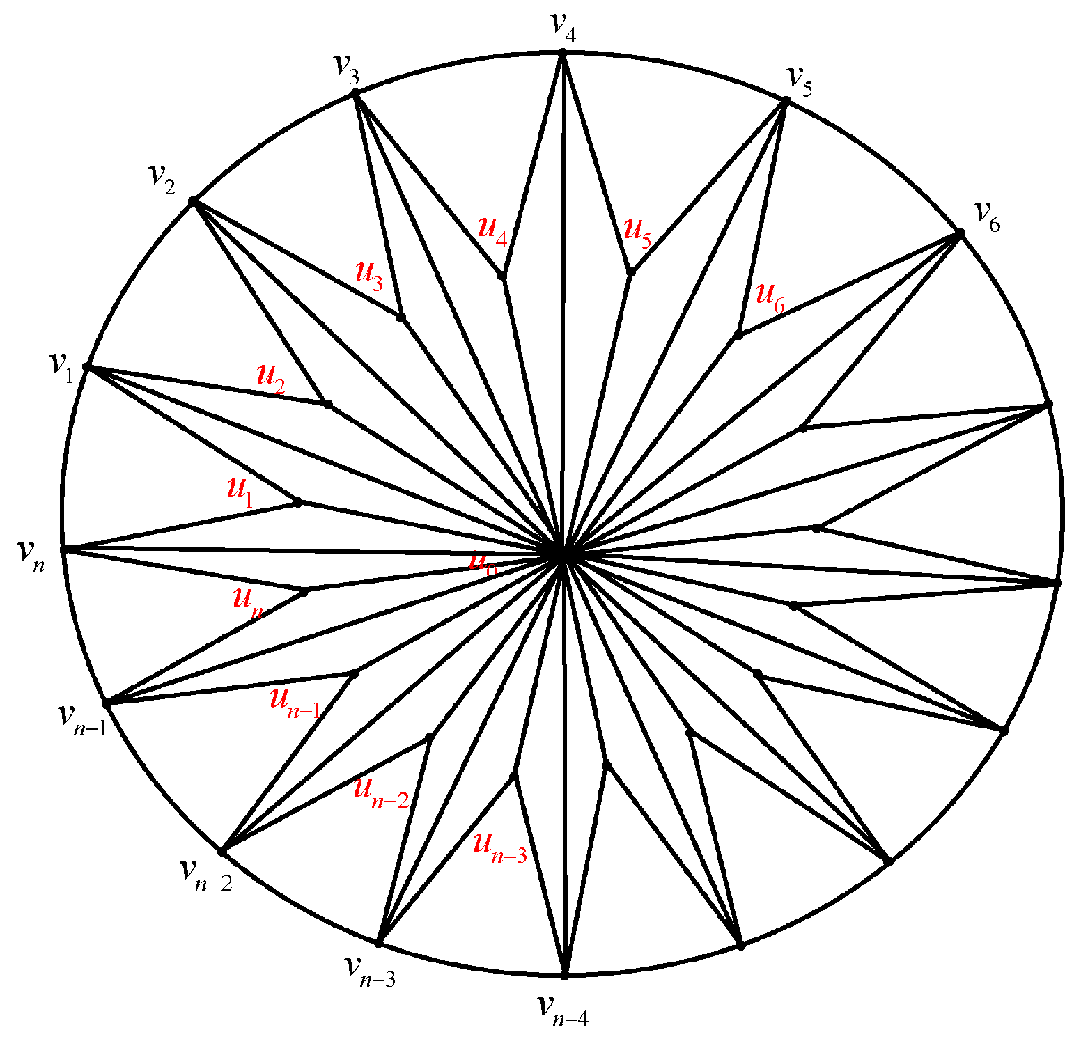
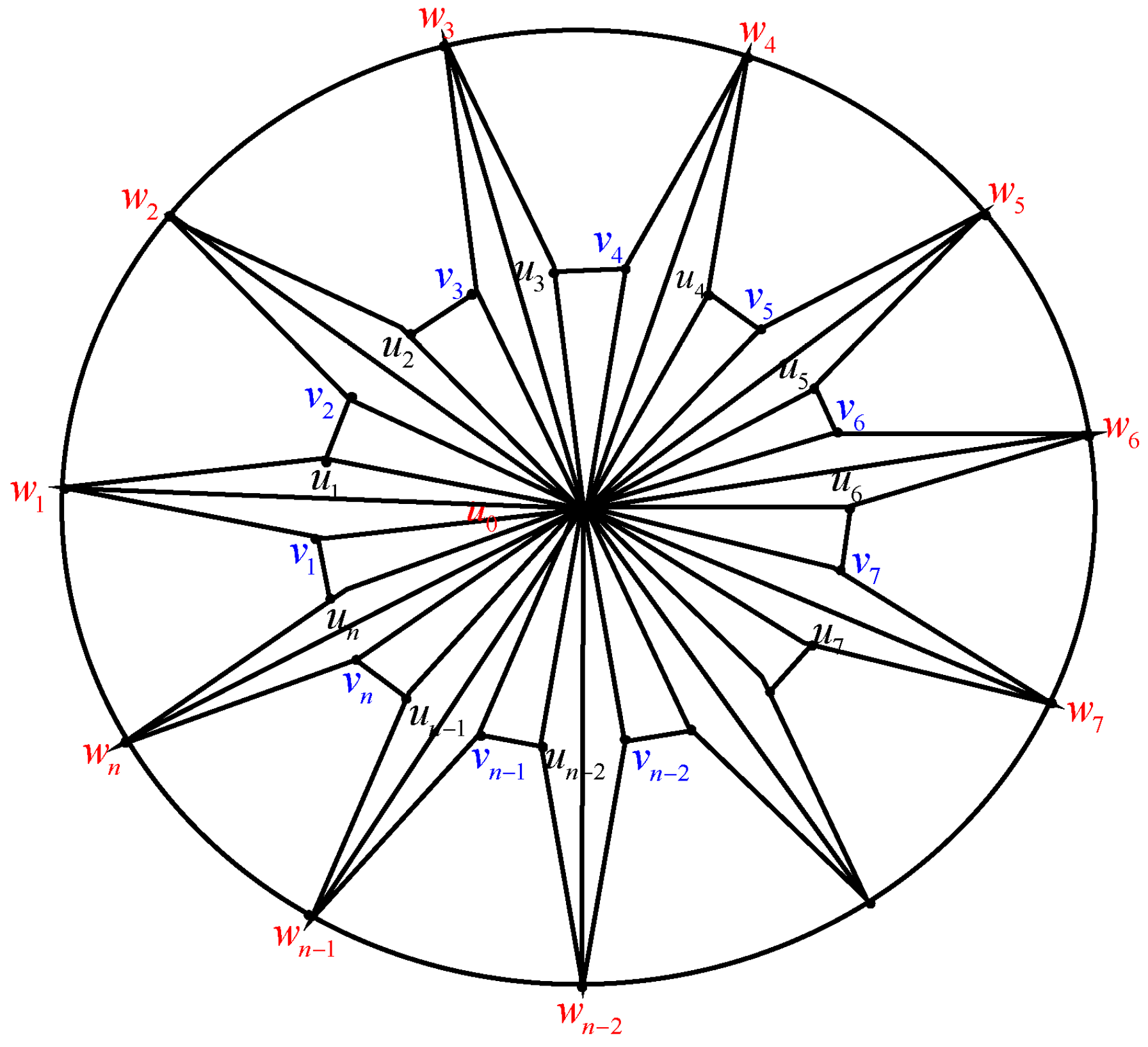
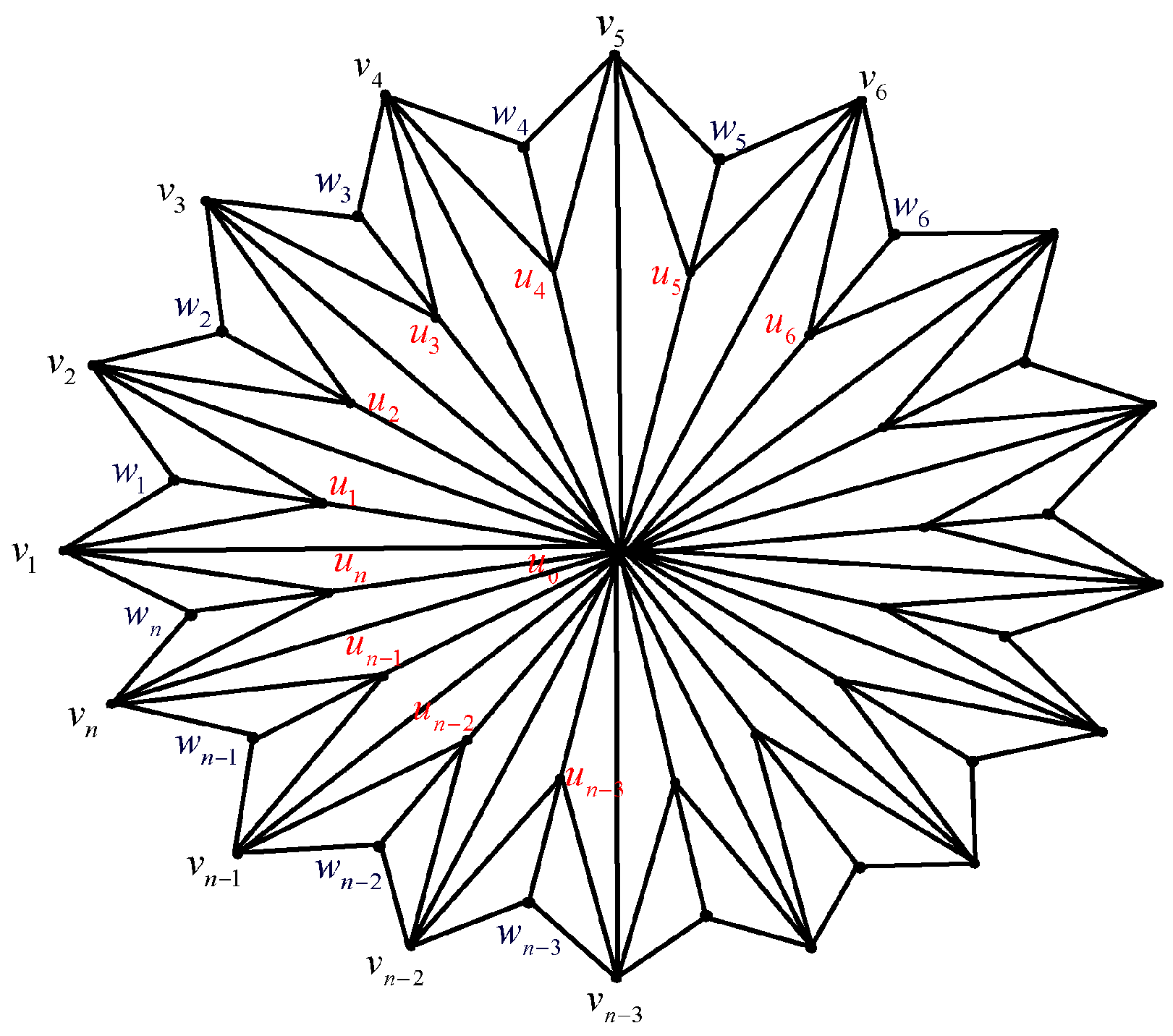
The closed cog double-star graph, ${CCDS}_n,$ is a graph that is created by combining the cycle graph $C_n=\left\{v_1,v_2,\dots ,v_n\right\}$ and the cog double-star graph, $C{DS}_n$, as illustrated in Figure 4.

Obviously, the closed cog double-star graph $CCD{S}_n$ has order $\left|V(CCD{S}_n)\right|=2n+1$ and size $\left|E(CCD{S}_n)\right|=5n$, and, hence, for large values of $n$, its average degree is $5$.

Theorem 4.

For $n\ge 3$, we have $\tau (CCD{S}_n)= ( {\displaystyle \frac{1}{2 }}{)}^n [(13+\sqrt{105}{)}^n+(13-\sqrt{105}{)}^n-2^{3n+1}]$.

Proof. 

The matrix tree theorem gives us

$$\tau (CCD{S}_n)=\mathit{det}\left(\begin{array}{cccccccccccc}3& 0& \dots & \dots & \dots & 0& -1& 0& \dots & \dots & 0& -1\\ 0& \ddots & \ddots & \ddots & \ddots & ⋮& -1& \ddots & \ddots & \ddots & \ddots & 0\\ ⋮& \ddots & \ddots & \ddots & \ddots & ⋮& 0& \ddots & \ddots & \ddots & \ddots & ⋮\\ ⋮& \ddots & \ddots & \ddots & \ddots & ⋮& ⋮& \ddots & \ddots & \ddots & \ddots & ⋮\\ ⋮& \ddots & \ddots & \ddots & \ddots & 0& 0& \ddots & 0& \ddots & \ddots & 0\\ 0& \dots & \dots & \dots & 0& 3& 0& \dots & \dots & 0& -1& -1\\ -1& -1& 0& \dots & \dots & 0& 5& -1& 0& \dots & \dots & -1\\ 0& \ddots & \ddots & \ddots & \ddots & ⋮& -1& \ddots & \ddots & \ddots & \ddots & 0\\ ⋮& \ddots & \ddots & \ddots & \ddots & ⋮& 0& \ddots & \ddots & \ddots & \ddots & ⋮\\ ⋮& \ddots & \ddots & \ddots & \ddots & 0& ⋮& \ddots & \ddots & \ddots & \ddots & 0\\ 0& \ddots & \ddots & \ddots & \ddots & -1& 0& \ddots & \ddots & \ddots & \ddots & -1\\ -1& 0& \dots & \dots & 0& -1& -1& 0& \dots & 0& -1& 5\end{array}\right)=\mathit{det}\left(\begin{array}{cc}P& Q\\ R& S\end{array}\right).$$

Using Lemma (2), we obtain

$$\begin{array}{cc}\hfill \tau \left(CCD{S}_n\right)& =detP\times \det \left[S-R{P}^{-1}Q\right]\hfill \\ & =3^n\times \mathit{det}\left(\begin{array}{cccccc}{\displaystyle \frac{13}{3}}& -{\displaystyle \frac{4}{3}}& 0& \dots & 0& -{\displaystyle \frac{4}{3}}\\ -{\displaystyle \frac{4}{3}}& \ddots & \ddots & \ddots & \ddots & 0\\ 0& \ddots & \ddots & \ddots & \ddots & ⋮\\ ⋮& \ddots & \ddots & \ddots & \ddots & 0\\ 0& \ddots & \ddots & \ddots & \ddots & -{\displaystyle \frac{4}{3}}\\ -{\displaystyle \frac{4}{3}}& 0& \dots & 0& -{\displaystyle \frac{4}{3}}& {\displaystyle \frac{13}{3}}\end{array}\right)=4^n\times \mathit{det}\left(\begin{array}{cccccc}{\displaystyle \frac{13}{4}}& -1& 0& \dots & 0& -1\\ -1& \ddots & \ddots & \ddots & \ddots & 0\\ 0& \ddots & \ddots & \ddots & \ddots & ⋮\\ ⋮& \ddots & \ddots & \ddots & \ddots & 0\\ 0& \ddots & \ddots & \ddots & \ddots & -1\\ -1& 0& \dots & 0& -1& {\displaystyle \frac{13}{4}}\end{array}\right).\hfill \end{array}$$

By using Lemma (1), we arrive at

$$\tau \left(CCD{S}_n\right)=4^n\times 2[T_n({\displaystyle \frac{13}{8}})-1].$$

The result follows from Equation (4). $\square$

Definition 5.

For $n\ge 3$, the water wheel graph, ${WW}_n$, is a graph with vertex set $V({WW}_n)$ = $\left\{u_0\right\}\cup \{u_i,v_i,w_i,i\le i\le n\}$ and edge set $E\left({WW}_n\right)$ = $\left\{u_0{u}_i,u_0{v}_i u_i{w}_i, v_i{w}_i:i\le i\le n \right\}\cup \left\{u_i{v}_{i+1}:i\le i\le n-1\right\}\cup \left\{u_n{v}_1\right\}.$ See Figure 5.

Obviously, the water wheel graph ${WW}_n$ has order $\left|V({WW}_n)\right|=3n+1$ and size $\left|E({WW}_n)\right|=5n$, and, hence, for large values of $n$, its average degree is $3.33$.

Theorem 5.

For $n\ge 3$, we have $\tau ({WW}_n)=(5+2\sqrt{6}{)}^n+(5-2\sqrt{6}{)}^n-2.$

Proof. 

From the matrix tree theorem, we have

$$\tau ({WW}_n)=\mathit{det}\left(\begin{array}{ccccccccccccccc}3& 0& \dots & \dots & 0& 0& -1& 0& \dots & 0& -1& 0& \dots & \dots & 0\\ 0& \ddots & \ddots & \ddots & ⋮& 0& \ddots & \ddots & \ddots & ⋮& 0& \ddots & \ddots & \ddots & ⋮\\ ⋮& \ddots & \ddots & \ddots & ⋮& ⋮& \ddots & \ddots & \ddots & 0& ⋮& \ddots & \ddots & \ddots & ⋮\\ ⋮& \ddots & \ddots & \ddots & 0& 0& \ddots & \ddots & \ddots & -1& ⋮& \ddots & \ddots & \ddots & 0\\ 0& \dots & \dots & 0& 3& -1& 0& \dots & 0& 0& 0& \dots & \dots & 0& -1\\ 0& \dots & \dots & 0& -1& 3& 0& \dots & \dots & 0& -1& 0& \dots & \dots & 0\\ -1& \ddots & \ddots & \ddots & 0& 0& \ddots & \ddots & \ddots & ⋮& 0& \ddots & \ddots & \ddots & ⋮\\ ⋮& \ddots & \ddots & \ddots & ⋮& ⋮& \ddots & \ddots & \ddots & ⋮& ⋮& \ddots & \ddots & \ddots & ⋮\\ ⋮& \ddots & \ddots & \ddots & ⋮& ⋮& \ddots & \ddots & \ddots & 0& ⋮& \ddots & \ddots & \ddots & 0\\ 0& \dots & 0& -1& 0& 0& \dots & \dots & 0& 3& 0& \dots & \dots & 0& -1\\ -1& 0& \dots & \dots & 0& -1& 0& \dots & \dots & 0& 2& 0& \dots & \dots & 0\\ 0& \ddots & \ddots & \ddots & ⋮& 0& \ddots & \ddots & \ddots & ⋮& 0& \ddots & \ddots & \ddots & ⋮\\ ⋮& \ddots & \ddots & \ddots & ⋮& ⋮& \ddots & \ddots & \ddots & ⋮& ⋮& \ddots & \ddots & \ddots & ⋮\\ ⋮& \ddots & \ddots & \ddots & 0& ⋮& \ddots & \ddots & \ddots & 0& ⋮& \ddots & \ddots & \ddots & 0\\ 0& \dots & \dots & 0& -1& 0& \dots & \dots & 0& -1& 0& \dots & \dots & 0& 2\end{array}\right)=\mathit{det}\left(\begin{array}{ccc}P& Q& T\\ R& S& U\\ V& W& X\end{array}\right).$$

Using Lemma (2), we obtain

$$\begin{array}{cc}\hfill \tau ({WW}_n)& =detX\times \mathrm{d}\mathrm{e}\mathrm{t}[ \left(\begin{array}{cc}P& Q\\ R& S\end{array}\right)-\left(\begin{array}{c}T\\ U\end{array}\right){P X}^{-1} \left(\begin{array}{cc}V& W\end{array}\right)]\hfill \\ & =2^n\times \mathit{det}\left(\begin{array}{cccccccccc}{\displaystyle \frac{5}{2}}& 0& \dots & \dots & 0& -{\displaystyle \frac{1}{2}}& -1& 0& \dots & 0\\ 0& \ddots & \ddots & \ddots & ⋮& 0& \ddots & \ddots & \ddots & ⋮\\ ⋮& \ddots & \ddots & \ddots & ⋮& ⋮& \ddots & \ddots & \ddots & 0\\ ⋮& \ddots & \ddots & \ddots & 0& 0& \ddots & \ddots & \ddots & -1\\ 0& \dots & \dots & 0& {\displaystyle \frac{5}{2}}& -1& 0& \dots & 0& -{\displaystyle \frac{1}{2}}\\ -{\displaystyle \frac{1}{2}}& 0& \dots & 0& -1& {\displaystyle \frac{5}{2}}& 0& \dots & \dots & 0\\ -1& \ddots & \ddots & \ddots & 0& 0& \ddots & \ddots & \ddots & ⋮\\ 0& \ddots & \ddots & \ddots & ⋮& ⋮& \ddots & \ddots & \ddots & ⋮\\ ⋮& \ddots & \ddots & \ddots & 0& ⋮& \ddots & \ddots & \ddots & 0\\ 0& \dots & 0& -1& -{\displaystyle \frac{1}{2}}& 0& \dots & \dots & 0& {\displaystyle \frac{5}{2}}\end{array}\right)\hfill \\ & ={\displaystyle \frac{1}{2^n}}\times \mathit{det}\left(\begin{array}{cccccccccc}5& 0& \dots & \dots & 0& -1& -2& 0& \dots & 0\\ 0& \ddots & \ddots & \ddots & ⋮& 0& \ddots & \ddots & \ddots & ⋮\\ ⋮& \ddots & \ddots & \ddots & ⋮& ⋮& \ddots & \ddots & \ddots & 0\\ ⋮& \ddots & \ddots & \ddots & 0& 0& \ddots & \ddots & \ddots & -2\\ 0& \dots & \dots & 0& 5& -2& 0& \dots & 0& -1\\ -1& 0& \dots & 0& -2& 5& 0& \dots & \dots & 0\\ -2& \ddots & \ddots & \ddots & 0& 0& \ddots & \ddots & \ddots & ⋮\\ 0& \ddots & \ddots & \ddots & ⋮& ⋮& \ddots & \ddots & \ddots & ⋮\\ ⋮& \ddots & \ddots & \ddots & 0& ⋮& \ddots & \ddots & \ddots & 0\\ 0& \dots & 0& -2& -1& 0& \dots & \dots & 0& 5\end{array}\right)=\mathit{det}\left( \begin{array}{cc}A& B\\ C& D\end{array}\right).\hfill \end{array}$$

By applying Lemma (2) once more, we get

$$\begin{array}{cc}\hfill \tau ({WW}_n)=& det A\times \mathrm{d}\mathrm{e}\mathrm{t}[ D-C{A}^{-1} B]\hfill \\ & ={\displaystyle \frac{5^n}{2^n}}\times \mathit{det}\left(\begin{array}{cccccc}4& -{\displaystyle \frac{2}{5}}& 0& \dots & 0& -{\displaystyle \frac{2}{5}}\\ -{\displaystyle \frac{2}{5}}& \ddots & \ddots & \ddots & \ddots & 0\\ 0& \ddots & \ddots & \ddots & \ddots & ⋮\\ ⋮& \ddots & \ddots & \ddots & \ddots & 0\\ 0& \ddots & \ddots & \ddots & \ddots & -{\displaystyle \frac{2}{5}}\\ --{\displaystyle \frac{2}{5}}& 0& \dots & 0& -{\displaystyle \frac{2}{5}}& 4\end{array}\right)=\mathit{det}\left(\begin{array}{cccccc}10& -1& 0& \dots & 0& -1\\ -1& \ddots & \ddots & \ddots & \ddots & 0\\ 0& \ddots & \ddots & \ddots & \ddots & ⋮\\ ⋮& \ddots & \ddots & \ddots & \ddots & 0\\ 0& \ddots & \ddots & \ddots & \ddots & -1\\ -1& 0& \dots & 0& -1& 10\end{array}\right).\hfill \end{array}$$

By using Lemma (1), we arrive at

$$\tau \left(CD{S}_n\right)=2[T_n(5)-1].$$

The result follows from Equation (4). $\square$

Definition 6.

For $n\ge 3$, the closed water wheel graph, ${CWW}_n$, is a graph obtained by adding edges $w_1{w}_n$ and $w_i{w}_{ni+1}$, $1\le i\le n-1$, to the water wheel graph ${WW}_n$. See Figure 6.

Obviously, the closed water wheel graph $C{WW}_n$ has order $\left|V({CWW}_n)\right|=3n+1$ and size $\left|E(\mathrm{C}{WW}_n)\right|=6n$, and, hence, for large values of $n$, its average degree is $4$.

Theorem 6.

For $n\ge 3$, we have $\tau (C{WW}_n)=(13+2\sqrt{22}{)}^n+(13-2\sqrt{22}{)}^n-2\times 9^n.$

Proof. 

From the matrix tree theorem, we have

$$\tau (C{WW}_n)=\mathit{det}\left(\begin{array}{cccccccccccccccccc}3& 0& \dots & \dots & 0& 0& 0& -1& 0& \dots & \dots & 0& -1& 0& \dots & \dots & \dots & 0\\ 0& \ddots & \ddots & \ddots & \ddots & ⋮& ⋮& \ddots & \ddots & \ddots & \ddots & ⋮& 0& \ddots & \ddots & \ddots & \ddots & ⋮\\ ⋮& \ddots & \ddots & \ddots & \ddots & ⋮& ⋮& \ddots & \ddots & \ddots & \ddots & ⋮& ⋮& \ddots & \ddots & \ddots & \ddots & ⋮\\ ⋮& \ddots & \ddots & \ddots & \ddots & ⋮& ⋮& \ddots & \ddots & \ddots & \ddots & 0& ⋮& \ddots & \ddots & \ddots & \ddots & ⋮\\ ⋮& \ddots & \ddots & \ddots & \ddots & 0& 0& \ddots & \ddots & \ddots & \ddots & -1& ⋮& \ddots & \ddots & \ddots & \ddots & 0\\ 0& \dots & \dots & \dots & 0& 3& -1& 0& \dots & \dots & \dots & 0& 0& \dots & \dots & \dots & 0& -1\\ 0& \dots & \dots & \dots & 0& -1& 3& 0& \dots & \dots & \dots & 0& -1& 0& \dots & \dots & \dots & 0\\ -1& \ddots & \ddots & \ddots & \ddots & 0& 0& \ddots & \ddots & \ddots & \ddots & ⋮& 0& \ddots & \ddots & \ddots & \ddots & ⋮\\ 0& \ddots & \ddots & \ddots & \ddots & ⋮& ⋮& \ddots & \ddots & \ddots & \ddots & ⋮& ⋮& \ddots & \ddots & \ddots & \ddots & ⋮\\ ⋮& \ddots & \ddots & \ddots & \ddots & ⋮& ⋮& \ddots & \ddots & \ddots & \ddots & ⋮& ⋮& \ddots & \ddots & \ddots & \ddots & ⋮\\ ⋮& \ddots & \ddots & \ddots & \ddots & ⋮& ⋮& \ddots & \ddots & \ddots & \ddots & 0& ⋮& \ddots & \ddots & \ddots & \ddots & 0\\ 0& \dots & \dots & 0& -1& 0& 0& \dots & \dots & \dots & 0& 3& 0& \dots & \dots & \dots & 0& -1\\ -1& 0& \dots & \dots & \dots & 0& -1& 0& \dots & \dots & \dots & 0& 4& -1& 0& \dots & 0& -1\\ 0& \ddots & \ddots & \ddots & \ddots & ⋮& 0& \ddots & \ddots & \ddots & \ddots & ⋮& -1& \ddots & \ddots & \ddots & \ddots & 0\\ ⋮& \ddots & \ddots & \ddots & \ddots & ⋮& ⋮& \ddots & \ddots & \ddots & \ddots & ⋮& 0& \ddots & \ddots & \ddots & \ddots & ⋮\\ ⋮& \ddots & \ddots & \ddots & \ddots & ⋮& ⋮& \ddots & \ddots & \ddots & \ddots & ⋮& ⋮& \ddots & \ddots & \ddots & \ddots & 0\\ ⋮& \ddots & \ddots & \ddots & \ddots & 0& ⋮& \ddots & \ddots & \ddots & \ddots & 0& 0& \ddots & \ddots & \ddots & \ddots & -1\\ 0& \dots & \dots & \dots & 0& -1& 0& \dots & \dots & \dots & 0& -1& -1& 0& \dots & 0& -1& 4\end{array}\right)=\mathit{det}\left(\begin{array}{ccc}P& Q& T\\ R& S& U\\ V& W& X\end{array}\right).$$

By applying Lemma (2), we obtain

$$\begin{array}{cc}\hfill \tau \left(C{WW}_n\right)& =det \left(\begin{array}{cc}P& Q\\ R& S\end{array}\right)\times \mathrm{d}\mathrm{e}\mathrm{t}[X-\left(\begin{array}{cc}V& W\end{array}\right){ \left(\begin{array}{cc}P& Q\\ R& S\end{array}\right)}^{-1}\left(\begin{array}{c}T\\ U\end{array}\right) ]\hfill \\ & =\mathit{det}\left(\begin{array}{cccccccccccc}3& 0& \dots & \dots & 0& 0& 0& -1& 0& \dots & \dots & 0\\ 0& \ddots & \ddots & \ddots & \ddots & ⋮& ⋮& \ddots & \ddots & \ddots & \ddots & ⋮\\ ⋮& \ddots & \ddots & \ddots & \ddots & ⋮& ⋮& \ddots & \ddots & \ddots & \ddots & ⋮\\ ⋮& \ddots & \ddots & \ddots & \ddots & ⋮& ⋮& \ddots & \ddots & \ddots & \ddots & 0\\ ⋮& \ddots & \ddots & \ddots & \ddots & 0& 0& \ddots & \ddots & \ddots & \ddots & -1\\ 0& \dots & \dots & \dots & 0& 3& -1& 0& \dots & \dots & \dots & 0\\ 0& \dots & \dots & \dots & 0& -1& 3& 0& \dots & \dots & \dots & 0\\ -1& \ddots & \ddots & \ddots & \ddots & 0& 0& \ddots & \ddots & \ddots & \ddots & ⋮\\ 0& \ddots & \ddots & \ddots & \ddots & ⋮& ⋮& \ddots & \ddots & \ddots & \ddots & ⋮\\ ⋮& \ddots & \ddots & \ddots & \ddots & ⋮& ⋮& \ddots & \ddots & \ddots & \ddots & ⋮\\ ⋮& \ddots & \ddots & \ddots & \ddots & ⋮& ⋮& \ddots & \ddots & \ddots & \ddots & 0\\ 0& \dots & \dots & 0& -1& 0& 0& \dots & \dots & \dots & 0& 3\end{array}\right)\times \mathit{det}\left(\begin{array}{cccccc}{\displaystyle \frac{13}{4}}& -{\displaystyle \frac{9}{8}}& \dots & \dots & 0& -{\displaystyle \frac{9}{8}}\\ -{\displaystyle \frac{9}{8}}& \ddots & \ddots & \ddots & \ddots & 0\\ 0& \ddots & \ddots & \ddots & \ddots & ⋮\\ ⋮& \ddots & \ddots & \ddots & \ddots & 0\\ 0& \ddots & \ddots & \ddots & \ddots & -{\displaystyle \frac{9}{8}}\\ -{\displaystyle \frac{9}{8}}& 0& \dots & 0& -{\displaystyle \frac{9}{8}}& {\displaystyle \frac{13}{4}}\end{array}\right)\hfill \end{array}.$$

By applying Lemma (4), we obtain

$$\tau \left(C{WW}_n\right)=\mathit{det}\left(\begin{array}{ccccc}8& 0& \dots & \dots & 0\\ 0& \ddots & \ddots & \ddots & ⋮\\ ⋮& \ddots & \ddots & \ddots & ⋮\\ ⋮& \ddots & \ddots & \ddots & 0\\ 0& \dots & \dots & 0& 8\end{array}\right)\times ({\displaystyle \frac{9}{8}}{)}^n\mathit{det}\left(\begin{array}{cccccc}{\displaystyle \frac{26}{9}}& -1& \dots & \dots & 0& -{\displaystyle \frac{9}{8}}\\ -1& \ddots & \ddots & \ddots & \ddots & 0\\ 0& \ddots & \ddots & \ddots & \ddots & ⋮\\ ⋮& \ddots & \ddots & \ddots & \ddots & 0\\ 0& \ddots & \ddots & \ddots & \ddots & -1\\ -1& 0& \dots & 0& -1& {\displaystyle \frac{26}{9}}\end{array}\right).$$

Using Lemma (1), we obtain

$$\tau \left(C{WW}_n\right)=9^n\times 2[T_n({\displaystyle \frac{13}{9}})-1].$$

The result follows from Equation (4). $\square$

Definition 7.

For $n\ge 3$, the triangulated water wheel graph, ${TWW}_n$, is a graph obtained by adding edges $u_0{w}_i$ for all $i\le i\le n-1$ to the water wheel graph ${WW}_n$. See Figure 7.

Obviously, the triangulated water wheel graph ${TWW}_n$ has order $\left|V({TWW}_n)\right|=3n+1$ and size $\left|E({TWW}_n)\right|=6n$, and, hence, for large values of $n$, its average degree is $4$.

Theorem 7.

For $n\ge 3$, we have $\tau ({TWW}_n)=(9+4\sqrt{5}{)}^n+(9-4\sqrt{5}{)}^n-2.$

Proof. 

From the matrix tree theorem, we have

$$\tau ({TWW}_n)=\mathit{det}\left(\begin{array}{ccccccccccccccc}3& 0& \dots & \dots & 0& 0& -1& 0& \dots & 0& -1& 0& \dots & \dots & 0\\ 0& \ddots & \ddots & \ddots & ⋮& 0& \ddots & \ddots & \ddots & ⋮& 0& \ddots & \ddots & \ddots & ⋮\\ ⋮& \ddots & \ddots & \ddots & ⋮& ⋮& \ddots & \ddots & \ddots & 0& ⋮& \ddots & \ddots & \ddots & ⋮\\ ⋮& \ddots & \ddots & \ddots & 0& 0& \ddots & \ddots & \ddots & -1& ⋮& \ddots & \ddots & \ddots & 0\\ 0& \dots & \dots & 0& 3& -1& 0& \dots & 0& 0& 0& \dots & \dots & 0& -1\\ 0& \dots & \dots & 0& -1& 3& 0& \dots & \dots & 0& -1& 0& \dots & \dots & 0\\ -1& \ddots & \ddots & \ddots & 0& 0& \ddots & \ddots & \ddots & ⋮& 0& \ddots & \ddots & \ddots & ⋮\\ ⋮& \ddots & \ddots & \ddots & ⋮& ⋮& \ddots & \ddots & \ddots & ⋮& ⋮& \ddots & \ddots & \ddots & ⋮\\ ⋮& \ddots & \ddots & \ddots & ⋮& ⋮& \ddots & \ddots & \ddots & 0& ⋮& \ddots & \ddots & \ddots & 0\\ 0& \dots & 0& -1& 0& 0& \dots & \dots & 0& 3& 0& \dots & \dots & 0& -1\\ -1& 0& \dots & \dots & 0& -1& 0& \dots & \dots & 0& 3& 0& \dots & \dots & 0\\ 0& \ddots & \ddots & \ddots & ⋮& 0& \ddots & \ddots & \ddots & ⋮& 0& \ddots & \ddots & \ddots & ⋮\\ ⋮& \ddots & \ddots & \ddots & ⋮& ⋮& \ddots & \ddots & \ddots & ⋮& ⋮& \ddots & \ddots & \ddots & ⋮\\ ⋮& \ddots & \ddots & \ddots & 0& ⋮& \ddots & \ddots & \ddots & 0& ⋮& \ddots & \ddots & \ddots & 0\\ 0& \dots & \dots & 0& -1& 0& \dots & \dots & 0& -1& 0& \dots & \dots & 0& 3\end{array}\right)=\mathit{det}\left(\begin{array}{ccc}P& Q& T\\ R& S& U\\ V& W& X\end{array}\right).$$

By applying Lemma (2), we obtain

$$\begin{array}{cc}\hfill \tau \left({TWW}_n\right)& =det X\times \mathrm{d}\mathrm{e}\mathrm{t}[\left(\begin{array}{cc}P& Q\\ R& S\end{array}\right)-{ \left(\begin{array}{c}T\\ U\end{array}\right) X}^{-1}\left(\begin{array}{cc}V& W\end{array}\right)\hfill \\ & =3^n\times \mathit{det}\left(\begin{array}{cccccccccc}{\displaystyle \frac{8}{3}}& 0& \dots & \dots & 0& -{\displaystyle \frac{1}{3}}& -1& 0& \dots & 0\\ 0& \ddots & \ddots & \ddots & ⋮& 0& \ddots & \ddots & \ddots & ⋮\\ ⋮& \ddots & \ddots & \ddots & ⋮& ⋮& \ddots & \ddots & \ddots & 0\\ ⋮& \ddots & \ddots & \ddots & 0& 0& \ddots & \ddots & \ddots & -1\\ 0& \dots & \dots & 0& {\displaystyle \frac{8}{3}}& -1& 0& \dots & 0& -{\displaystyle \frac{1}{3}}\\ -{\displaystyle \frac{1}{3}}& 0& \dots & 0& -1& {\displaystyle \frac{8}{3}}& 0& \dots & \dots & 0\\ -1& \ddots & \ddots & \ddots & 0& 0& \ddots & \ddots & \ddots & ⋮\\ 0& \ddots & \ddots & \ddots & ⋮& ⋮& \ddots & \ddots & \ddots & ⋮\\ ⋮& \ddots & \ddots & \ddots & 0& ⋮& \ddots & \ddots & \ddots & 0\\ 0& \dots & 0& -1& -{\displaystyle \frac{1}{3}}& 0& \dots & \dots & 0& {\displaystyle \frac{8}{3}}\end{array}\right)\hfill \\ & ={\displaystyle \frac{1}{3^n}}\times \mathit{det}\left(\begin{array}{cccccccccc}8& 0& \dots & \dots & 0& -1& -3& 0& \dots & 0\\ 0& \ddots & \ddots & \ddots & ⋮& 0& \ddots & \ddots & \ddots & ⋮\\ ⋮& \ddots & \ddots & \ddots & ⋮& ⋮& \ddots & \ddots & \ddots & 0\\ ⋮& \ddots & \ddots & \ddots & 0& 0& \ddots & \ddots & \ddots & -3\\ 0& \dots & \dots & 0& 8& -3& 0& \dots & 0& -1\\ -1& 0& \dots & 0& -3& 8& 0& \dots & \dots & 0\\ -3& \ddots & \ddots & \ddots & 0& 0& \ddots & \ddots & \ddots & ⋮\\ 0& \ddots & \ddots & \ddots & ⋮& ⋮& \ddots & \ddots & \ddots & ⋮\\ ⋮& \ddots & \ddots & \ddots & 0& ⋮& \ddots & \ddots & \ddots & 0\\ 0& \dots & 0& -3& -1& 0& \dots & \dots & 0& 8\end{array}\right)={\displaystyle \frac{1}{3^n}}\times \mathit{det}\left( \begin{array}{cc}A& B\\ B^t& A\end{array}\right)\hfill \end{array}.$$

By using Lemma (2), we get $\tau (T{WW}_n)=det A\times \mathrm{d}\mathrm{e}\mathrm{t}[ A-B{A}^{-1} B^t]$. Thus

$$\tau \left({TWW}_n\right)={\displaystyle \frac{8^n}{3^n}}\times \mathit{det}\left(\begin{array}{cccccc}{\displaystyle \frac{27}{4}}& -{\displaystyle \frac{3}{8}}& 0& \dots & 0& -{\displaystyle \frac{3}{8}}\\ -{\displaystyle \frac{3}{8}}& \ddots & \ddots & \ddots & \ddots & 0\\ 0& \ddots & \ddots & \ddots & \ddots & ⋮\\ ⋮& \ddots & \ddots & \ddots & \ddots & 0\\ 0& \ddots & \ddots & \ddots & \ddots & -{\displaystyle \frac{3}{8}}\\ -{\displaystyle \frac{3}{8}}& 0& \dots & 0& -{\displaystyle \frac{3}{8}}& {\displaystyle \frac{27}{4}}\end{array}\right)=\mathit{det}\left(\begin{array}{cccccc}18& -1& 0& \dots & 0& -1\\ -1& \ddots & \ddots & \ddots & \ddots & 0\\ 0& \ddots & \ddots & \ddots & \ddots & ⋮\\ ⋮& \ddots & \ddots & \ddots & \ddots & 0\\ 0& \ddots & \ddots & \ddots & \ddots & -1\\ -1& 0& \dots & 0& -1& 18\end{array}\right).$$

Using Lemma (1), we obtain

$$\tau \left({TWW}_n\right)=2[T_n(9)-1].$$

The result follows from Equation (4). $\square$

Definition 8.

For $n\ge 3$, the closed triangulated water wheel graph, ${CTWW}_n$, is a graph obtained by adding edges $w_1{w}_n$ and $w_i{w}_{i+1}$ for all $i\le i\le n-1$ to the triangulated water wheel graph ${TWW}_n$. See Figure 8.

Obviously, the closed triangulated water wheel graph $C{TWW}_n$ has order $\left|V({CTWW}_n)\right|=3n+1$ and size $\left|E(\mathrm{C}{TWW}_n)\right|=7n$, and, hence, for large values of $n$, its average degree is $4.66$.

Theorem 8.

For $n\ge 3$, we have $\tau (C{TWW}_n )=(17+2\sqrt{52}{)}^n+(17-2\sqrt{52}{)}^n-2\times 9^n$.

Proof. 

From the matrix tree theorem, we have

$$\tau \left(\mathrm{C}{TWW}_n\right)=\mathit{det}\left(\begin{array}{cccccccccccccccccc}3& 0& \dots & \dots & 0& 0& 0& -1& 0& \dots & \dots & 0& -1& 0& \dots & \dots & \dots & 0\\ 0& \ddots & \ddots & \ddots & \ddots & ⋮& ⋮& \ddots & \ddots & \ddots & \ddots & ⋮& 0& \ddots & \ddots & \ddots & \ddots & ⋮\\ ⋮& \ddots & \ddots & \ddots & \ddots & ⋮& ⋮& \ddots & \ddots & \ddots & \ddots & ⋮& ⋮& \ddots & \ddots & \ddots & \ddots & ⋮\\ ⋮& \ddots & \ddots & \ddots & \ddots & ⋮& ⋮& \ddots & \ddots & \ddots & \ddots & 0& ⋮& \ddots & \ddots & \ddots & \ddots & ⋮\\ ⋮& \ddots & \ddots & \ddots & \ddots & 0& 0& \ddots & \ddots & \ddots & \ddots & -1& ⋮& \ddots & \ddots & \ddots & \ddots & 0\\ 0& \dots & \dots & \dots & 0& 3& -1& 0& \dots & \dots & \dots & 0& 0& \dots & \dots & \dots & 0& -1\\ 0& \dots & \dots & \dots & 0& -1& 3& 0& \dots & \dots & \dots & 0& -1& 0& \dots & \dots & \dots & 0\\ -1& \ddots & \ddots & \ddots & \ddots & 0& 0& \ddots & \ddots & \ddots & \ddots & ⋮& 0& \ddots & \ddots & \ddots & \ddots & ⋮\\ 0& \ddots & \ddots & \ddots & \ddots & ⋮& ⋮& \ddots & \ddots & \ddots & \ddots & ⋮& ⋮& \ddots & \ddots & \ddots & \ddots & ⋮\\ ⋮& \ddots & \ddots & \ddots & \ddots & ⋮& ⋮& \ddots & \ddots & \ddots & \ddots & ⋮& ⋮& \ddots & \ddots & \ddots & \ddots & ⋮\\ ⋮& \ddots & \ddots & \ddots & \ddots & ⋮& ⋮& \ddots & \ddots & \ddots & \ddots & 0& ⋮& \ddots & \ddots & \ddots & \ddots & 0\\ 0& \dots & \dots & 0& -1& 0& 0& \dots & \dots & \dots & 0& 3& 0& \dots & \dots & \dots & 0& -1\\ -1& 0& \dots & \dots & \dots & 0& -1& 0& \dots & \dots & \dots & 0& 5& -1& 0& \dots & 0& -1\\ 0& \ddots & \ddots & \ddots & \ddots & ⋮& 0& \ddots & \ddots & \ddots & \ddots & ⋮& -1& \ddots & \ddots & \ddots & \ddots & 0\\ ⋮& \ddots & \ddots & \ddots & \ddots & ⋮& ⋮& \ddots & \ddots & \ddots & \ddots & ⋮& 0& \ddots & \ddots & \ddots & \ddots & ⋮\\ ⋮& \ddots & \ddots & \ddots & \ddots & ⋮& ⋮& \ddots & \ddots & \ddots & \ddots & ⋮& ⋮& \ddots & \ddots & \ddots & \ddots & 0\\ ⋮& \ddots & \ddots & \ddots & \ddots & 0& ⋮& \ddots & \ddots & \ddots & \ddots & 0& 0& \ddots & \ddots & \ddots & \ddots & -1\\ 0& \dots & \dots & \dots & 0& -1& 0& \dots & \dots & \dots & 0& -1& -1& 0& \dots & 0& -1& 5\end{array}\right)=\mathit{det}\left(\begin{array}{ccc}P& Q& T\\ R& S& U\\ V& W& X\end{array}\right).$$

By applying Lemma (2), we obtain

$$\begin{array}{cc}\hfill \tau \left(C{TWW}_n\right)& =det \left(\begin{array}{cc}P& Q\\ R& S\end{array}\right)\times \mathrm{d}\mathrm{e}\mathrm{t}[ X-{ \left(\begin{array}{cc}V& W\end{array}\right) \left(\begin{array}{cc}P& Q\\ R& S\end{array}\right)}^{-1}\left(\begin{array}{c}T\\ U\end{array}\right) ]\hfill \\ & =\mathit{det}\left(\begin{array}{cccccccccccc}3& 0& \dots & \dots & 0& 0& 0& -1& 0& \dots & \dots & 0\\ 0& \ddots & \ddots & \ddots & \ddots & ⋮& ⋮& \ddots & \ddots & \ddots & \ddots & ⋮\\ ⋮& \ddots & \ddots & \ddots & \ddots & ⋮& ⋮& \ddots & \ddots & \ddots & \ddots & ⋮\\ ⋮& \ddots & \ddots & \ddots & \ddots & ⋮& ⋮& \ddots & \ddots & \ddots & \ddots & 0\\ ⋮& \ddots & \ddots & \ddots & \ddots & 0& 0& \ddots & \ddots & \ddots & \ddots & -1\\ 0& \dots & \dots & \dots & 0& 3& -1& 0& \dots & \dots & \dots & 0\\ 0& \dots & \dots & \dots & 0& -1& 3& 0& \dots & \dots & \dots & 0\\ -1& \ddots & \ddots & \ddots & \ddots & 0& 0& \ddots & \ddots & \ddots & \ddots & ⋮\\ 0& \ddots & \ddots & \ddots & \ddots & ⋮& ⋮& \ddots & \ddots & \ddots & \ddots & ⋮\\ ⋮& \ddots & \ddots & \ddots & \ddots & ⋮& ⋮& \ddots & \ddots & \ddots & \ddots & ⋮\\ ⋮& \ddots & \ddots & \ddots & \ddots & ⋮& ⋮& \ddots & \ddots & \ddots & \ddots & 0\\ 0& \dots & \dots & 0& -1& 0& 0& \dots & \dots & \dots & 0& 3\end{array}\right)\times \mathit{det}\left(\begin{array}{cccccc}{\displaystyle \frac{17}{4}}& -{\displaystyle \frac{9}{8}}& \dots & \dots & 0& -{\displaystyle \frac{9}{8}}\\ -{\displaystyle \frac{9}{8}}& \ddots & \ddots & \ddots & \ddots & 0\\ 0& \ddots & \ddots & \ddots & \ddots & ⋮\\ ⋮& \ddots & \ddots & \ddots & \ddots & 0\\ 0& \ddots & \ddots & \ddots & \ddots & -{\displaystyle \frac{9}{8}}\\ -{\displaystyle \frac{9}{8}}& 0& \dots & 0& -{\displaystyle \frac{9}{8}}& {\displaystyle \frac{17}{4}}\end{array}\right).\hfill \end{array}$$

By applying Lemma (4), we obtain

$$\tau \left(C{TWW}_n\right)=8^n\times ( {\displaystyle \frac{9}{8}}{ )}^n\mathit{det}\left(\begin{array}{cccccc}{\displaystyle \frac{34}{9}}& -1& \dots & \dots & 0& -{\displaystyle \frac{9}{8}}\\ -1& \ddots & \ddots & \ddots & \ddots & 0\\ 0& \ddots & \ddots & \ddots & \ddots & ⋮\\ ⋮& \ddots & \ddots & \ddots & \ddots & 0\\ 0& \ddots & \ddots & \ddots & \ddots & -1\\ -1& 0& \dots & 0& -1& {\displaystyle \frac{34}{9}}\end{array}\right).$$

Using Lemma (1), we obtain

$$\tau \left(C{TWW}_n\right)=9^n\times 2[T_n({\displaystyle \frac{17}{9}})-1].$$

The result follows from Equation (4). $\square$

Definition 9.

The cog wheel star graph, ${CWS}_n$, is a graph composed of a wheel graph $W_{2n}=\left\{u_0,u_1,v_1,u_2,v_2,\dots ,u_{n },v_n\right\}$ and a star $S_n=\{w_1,w_2,\dots ,w_n\}$ such that, for $1\le i\le n$, vertex $w_i$ is adjacent to vertices $u_i$ and $v_i$. Moreover, every vertex $w_i$ is adjacent to vertex $u_0$. See Figure 9.

Obviously, the cog wheel star graph ${CWS}_n$ has order $\left|V({CWS}_n)\right|=3n+1$ and size $\left|E({CWS}_n)\right|=7n$, and, hence, for large values of $n$, its average degree is $4.66$.

Theorem 9.

For $n\ge 3$, we have $\tau \left({CWS}_n\right)=4^n[(4+\sqrt{15}{)}^n+(4-\sqrt{15}{)}^n-2].$

Proof. 

From the matrix tree theorem, we have

$$\tau \left({CWS}_n\right)=\mathit{det}\left(\begin{array}{ccccccccccccccc}4& 0& \dots & \dots & 0& -1& 0& \dots & 0& -1& -1& 0& \dots & \dots & 0\\ 0& \ddots & \ddots & \ddots & ⋮& -1& \ddots & \ddots & \ddots & 0& 0& \ddots & \ddots & \ddots & ⋮\\ ⋮& \ddots & \ddots & \ddots & ⋮& 0& \ddots & \ddots & \ddots & ⋮& ⋮& \ddots & \ddots & \ddots & ⋮\\ ⋮& \ddots & \ddots & \ddots & 0& ⋮& \ddots & \ddots & \ddots & 0& ⋮& \ddots & \ddots & \ddots & 0\\ 0& \dots & \dots & 0& 4& 0& \dots & 0& -1& -1& 0& \dots & \dots & 0& -1\\ -1& -1& 0& \dots & 0& 4& 0& \dots & \dots & 0& -1& 0& \dots & \dots & 0\\ 0& \ddots & \ddots & \ddots & ⋮& 0& \ddots & \ddots & \ddots & ⋮& 0& \ddots & \ddots & \ddots & ⋮\\ ⋮& \ddots & \ddots & \ddots & 0& ⋮& \ddots & \ddots & \ddots & ⋮& ⋮& \ddots & \ddots & \ddots & ⋮\\ 0& \ddots & \ddots & \ddots & -1& ⋮& \ddots & \ddots & \ddots & 0& ⋮& \ddots & \ddots & \ddots & 0\\ -1& 0& \dots & 0& -1& 0& \dots & \dots & 0& 4& 0& \dots & \dots & 0& -1\\ -1& 0& \dots & \dots & 0& -1& 0& \dots & \dots & 0& 3& 0& \dots & \dots & 0\\ 0& \ddots & \ddots & \ddots & ⋮& 0& \ddots & \ddots & \ddots & ⋮& 0& \ddots & \ddots & \ddots & ⋮\\ ⋮& \ddots & \ddots & \ddots & ⋮& ⋮& \ddots & \ddots & \ddots & ⋮& ⋮& \ddots & \ddots & \ddots & ⋮\\ ⋮& \ddots & \ddots & \ddots & 0& ⋮& \ddots & \ddots & \ddots & 0& ⋮& \ddots & \ddots & \ddots & 0\\ 0& \dots & \dots & 0& -1& 0& \dots & \dots & 0& -1& 0& \dots & \dots & 0& 3\end{array}\right)=\mathit{det}\left(\begin{array}{ccc}P& Q& T\\ R& S& U\\ V& W& X\end{array}\right).$$

By applying Lemma (2), we obtain

$$\begin{array}{cc}\hfill \tau \left({CWS}_n\right)& =det X\times \mathrm{d}\mathrm{e}\mathrm{t}[ \left(\begin{array}{cc}P& Q\\ R& S\end{array}\right)-{ \left(\begin{array}{c}T\\ U\end{array}\right) X}^{-1} \left(\begin{array}{cc}V& W\end{array}\right) ]\hfill \\ & =3^n\times \mathit{det}\left(\begin{array}{cccccccccc}{\displaystyle \frac{11}{3}}& 0& \dots & \dots & 0& -{\displaystyle \frac{4}{3}}& 0& \dots & 0& -1\\ 0& \ddots & \ddots & \ddots & ⋮& -1& \ddots & \ddots & \ddots & 0\\ ⋮& \ddots & \ddots & \ddots & ⋮& 0& \ddots & \ddots & \ddots & ⋮\\ ⋮& \ddots & \ddots & \ddots & 0& ⋮& \ddots & \ddots & \ddots & 0\\ 0& \dots & \dots & 0& {\displaystyle \frac{11}{3}}& 0& \dots & 0& -1& -{\displaystyle \frac{4}{3}}\\ -{\displaystyle \frac{4}{3}}& -1& 0& \dots & 0& {\displaystyle \frac{11}{3}}& 0& \dots & \dots & 0\\ 0& \ddots & \ddots & \ddots & ⋮& 0& \ddots & \ddots & \ddots & ⋮\\ ⋮& \ddots & \ddots & \ddots & 0& ⋮& \ddots & \ddots & \ddots & ⋮\\ 0& \ddots & \ddots & \ddots & -1& ⋮& \ddots & \ddots & \ddots & 0\\ -1& 0& \dots & 0& -{\displaystyle \frac{4}{3}}& 0& \dots & \dots & 0& {\displaystyle \frac{11}{3}}\end{array}\right)=3^n\times \mathit{det}\left( \begin{array}{cc}A& B\\ B^t& A\end{array} \right).\hfill \end{array}$$

By applying Lemma (3), we obtain

$$\begin{array}{cc}\hfill \tau \left({CWS}_n\right)& =3^n\times \mathrm{d}\mathrm{e}\mathrm{t}[ A^2-B B^t ]\hfill \\ & =3^n\times \mathit{det}\left(\begin{array}{cccccc}{\displaystyle \frac{32}{3}}& -{\displaystyle \frac{4}{3}}& 0& \dots & 0& -{\displaystyle \frac{4}{3}}\\ -{\displaystyle \frac{4}{3}}& \ddots & \ddots & \ddots & \ddots & 0\\ 0& \ddots & \ddots & \ddots & \ddots & ⋮\\ ⋮& \ddots & \ddots & \ddots & \ddots & 0\\ 0& \ddots & \ddots & \ddots & \ddots & -{\displaystyle \frac{4}{3}}\\ -{\displaystyle \frac{4}{3}}& 0& \dots & 0& -{\displaystyle \frac{4}{3}}& {\displaystyle \frac{32}{3}}\end{array}\right)=4^n\times \mathit{det}\left(\begin{array}{cccccc}8& -1& 0& \dots & 0& -1\\ -1& \ddots & \ddots & \ddots & \ddots & 0\\ 0& \ddots & \ddots & \ddots & \ddots & ⋮\\ ⋮& \ddots & \ddots & \ddots & \ddots & 0\\ 0& \ddots & \ddots & \ddots & \ddots & -1\\ -1& 0& \dots & 0& -1& 8\end{array}\right).\hfill \end{array}$$

Using Lemma (1), we obtain

$$\tau \left({CWS}_n\right)=4^n\times 2[T_n(4)-1]$$

The result follows from Equation (4). $\square$

Definition 10.

For $n\ge 3,$ the double-cog star graph, or $DC{S}_n$, is a graph that is created by joining a star graph $S_n$ with a vertex set $V(S_n)=\{u_0,u_1,u_2,\dots ,u_n\}$ with two sets of vertices, {$v_1,v_2,\dots ,v_n\}$ and {$w_1,w_2,\dots ,w_n\},$ so that for $1\le i\le n-1$, vertex $u_i$ is adjacent to vertices $v_i$ and $v_{i+1}$, and $u_n$ is adjacent to $v_1$ and $v_n$. Furthermore, $w_i$ is adjacent to vertices $v_i$ and $v_{i+1}$, $w_n$ is adjacent to $v_1$ and $v_n$, and for $1\le i\le n$, $u_i$ is adjacent to $w_i$. See Figure 10.

Obviously, the double-cog star graph $DC{S}_n$ has order $\left|V(DC{S}_n)\right|=3n+1$ and size $\left|E(DC{S}_n)\right|=6n$, and, hence, for large values of $n$, its average degree is $4$.

Theorem 10.

For $n\ge 3$, we have $\tau \left(DC{S}_n\right)=(13+2\sqrt{22}{)}^n+(13-2\sqrt{22}{)}^n-2\times 9^n$.

Proof. 

From the matrix tree theorem, we have

$$\tau (DC{S}_n)=\mathit{det}\left(\begin{array}{ccccccccccccccc}4& 0& \dots & \dots & 0& -1& -1& 0& \dots & 0& -1& 0& \dots & \dots & 0\\ 0& \ddots & \ddots & \ddots & ⋮& 0& \ddots & \ddots & \ddots & ⋮& 0& \ddots & \ddots & \ddots & ⋮\\ ⋮& \ddots & \ddots & \ddots & ⋮& ⋮& \ddots & \ddots & \ddots & 0& ⋮& \ddots & \ddots & \ddots & ⋮\\ ⋮& \ddots & \ddots & \ddots & 0& 0& \ddots & \ddots & \ddots & -1& ⋮& \ddots & \ddots & \ddots & 0\\ 0& \dots & \dots & 0& 4& -1& 0& \dots & 0& -1& 0& \dots & \dots & 0& -1\\ -1& 0& \dots & 0& -1& 4& 0& \dots & \dots & 0& -1& 0& \dots & 0& -1\\ -1& \ddots & \ddots & \ddots & 0& 0& \ddots & \ddots & \ddots & ⋮& -1& \ddots & \ddots & \ddots & 0\\ 0& \ddots & \ddots & \ddots & ⋮& ⋮& \ddots & \ddots & \ddots & ⋮& 0& \ddots & \ddots & \ddots & ⋮\\ ⋮& \ddots & \ddots & \ddots & 0& ⋮& \ddots & \ddots & \ddots & 0& ⋮& \ddots & \ddots & \ddots & 0\\ 0& \dots & 0& -1& -1& 0& \dots & \dots & 0& 4& 0& \dots & 0& -1& -1\\ -1& 0& \dots & \dots & 0& -1& -1& 0& \dots & 0& 3& 0& \dots & \dots & 0\\ 0& \ddots & \ddots & \ddots & ⋮& 0& \ddots & \ddots & \ddots & ⋮& 0& \ddots & \ddots & \ddots & ⋮\\ ⋮& \ddots & \ddots & \ddots & ⋮& ⋮& \ddots & \ddots & \ddots & 0& ⋮& \ddots & \ddots & \ddots & ⋮\\ ⋮& \ddots & \ddots & \ddots & 0& 0& \ddots & \ddots & \ddots & -1& ⋮& \ddots & \ddots & \ddots & 0\\ 0& \dots & \dots & 0& -1& -1& 0& \dots & 0& -1& 0& \dots & \dots & 0& 3\end{array}\right)=\mathit{det}\left(\begin{array}{ccc}P& Q& T\\ R& S& U\\ V& W& X\end{array}\right).$$

By applying Lemma (2), we obtain

$$\begin{array}{cc}\hfill \tau \left(DC{S}_n\right)& =det X\times \mathrm{d}\mathrm{e}\mathrm{t}[ \left(\begin{array}{cc}P& Q\\ R& S\end{array}\right)-{ \left(\begin{array}{c}T\\ U\end{array}\right) X}^{-1} \left(\begin{array}{cc}V& W\end{array}\right) ]\hfill \\ & =3^n\times \mathit{det}\left(\begin{array}{cccccccccccc}{\displaystyle \frac{11}{3}}& 0& \dots & \dots & 0& 0& -{\displaystyle \frac{4}{3}}& -{\displaystyle \frac{4}{3}}& 0& \dots & \dots & 0\\ 0& \ddots & \ddots & \ddots & \ddots & ⋮& 0& \ddots & \ddots & \ddots & \ddots & ⋮\\ ⋮& \ddots & \ddots & \ddots & \ddots & ⋮& ⋮& \ddots & \ddots & \ddots & \ddots & ⋮\\ ⋮& \ddots & \ddots & \ddots & \ddots & ⋮& ⋮& \ddots & \ddots & \ddots & \ddots & 0\\ ⋮& \ddots & \ddots & \ddots & \ddots & 0& 0& \ddots & \ddots & \ddots & \ddots & -{\displaystyle \frac{4}{3}}\\ 0& \dots & \dots & \dots & 0& {\displaystyle \frac{11}{3}}& -{\displaystyle \frac{4}{3}}& 0& \dots & \dots & 0& -{\displaystyle \frac{4}{3}}\\ -{\displaystyle \frac{4}{3}}& 0& \dots & \dots & 0& -{\displaystyle \frac{4}{3}}& {\displaystyle \frac{10}{3}}& -{\displaystyle \frac{1}{3}}& 0& \dots & 0& -{\displaystyle \frac{1}{3}}\\ -{\displaystyle \frac{4}{3}}& \ddots & \ddots & \ddots & \ddots & 0& -{\displaystyle \frac{1}{3}}& \ddots & \ddots & \ddots & \ddots & 0\\ 0& \ddots & \ddots & \ddots & \ddots & ⋮& 0& \ddots & \ddots & \ddots & \ddots & ⋮\\ ⋮& \ddots & \ddots & \ddots & \ddots & ⋮& ⋮& \ddots & \ddots & \ddots & \ddots & 0\\ ⋮& \ddots & \ddots & \ddots & \ddots & 0& 0& \ddots & \ddots & \ddots & \ddots & -{\displaystyle \frac{1}{3}}\\ 0& \dots & \dots & 0& -{\displaystyle \frac{4}{3}}& -{\displaystyle \frac{4}{3}}& -{\displaystyle \frac{1}{3}}& 0& \dots & 0& -{\displaystyle \frac{1}{3}}& {\displaystyle \frac{10}{3}}\end{array}\right)=3^n\times \mathit{det}\left( \begin{array}{cc}A& B\\ B^t& A\end{array}\right).\hfill \end{array}$$

By applying Lemma (3), we obtain

$$\tau \left(DC{S}_n\right)=3^n\times \mathrm{d}\mathrm{e}\mathrm{t}[ A^2-B B^t ]=3^n\mathit{det}\left(\begin{array}{cccccc}{\displaystyle \frac{26}{3}}& -3& 0& \dots & 0& -3\\ -3& \ddots & \ddots & \ddots & \ddots & 0\\ 0& \ddots & \ddots & \ddots & \ddots & ⋮\\ ⋮& \ddots & \ddots & \ddots & \ddots & 0\\ 0& \ddots & \ddots & \ddots & \ddots & -3\\ -3& 0& \dots & 0& -3& {\displaystyle \frac{26}{3}}\end{array}\right)=9^n\mathit{det}\left(\begin{array}{cccccc}{\displaystyle \frac{26}{9}}& -1& 0& \dots & 0& -1\\ -1& \ddots & \ddots & \ddots & \ddots & 0\\ 0& \ddots & \ddots & \ddots & \ddots & ⋮\\ ⋮& \ddots & \ddots & \ddots & \ddots & 0\\ 0& \ddots & \ddots & \ddots & \ddots & -1\\ -1& 0& \dots & 0& -1& {\displaystyle \frac{26}{9}}\end{array}\right).$$

Using Lemma (1), we obtain

$$\tau \left(DC{S}_n\right)=9^n\times 2[T_n({\displaystyle \frac{13}{9}})-1].$$

The result follows from Equation (4). $\square$

Definition 11.

For $n\ge 3$, the closed double-cog star graph, or $CDC{S}_n$, is a graph obtained by adding edges $v_1{v}_n$ and $v_i{v}_{i+1}$ for all $i\le i\le n-1$ to the double-cog star graph $DC{S}_n$. See Figure 11.

Obviously, the closed double-cog star graph $CDC{S}_n$ has order $\left|V(CDC{S}_n)\right|=3n+1$ and size $\left|E(CDC{S}_n)\right|=7n$, and, hence, for large values of $n$, its average degree is $4.66$.

Theorem 11.

For $n\ge 3$, we have $\tau \left(CDC{S}_n\right)=4^n[(6+\sqrt{11}{)}^n+(6-\sqrt{11}{)}^n-2\times 5^n]$.

Proof. 

From the matrix tree theorem, we have

$$\tau (CDC{S}_n)=\mathit{det}\left(\begin{array}{cccccccccccccccccc}4& 0& \dots & \dots & \dots & 0& -1& -1& 0& \dots & \dots & 0& -1& 0& \dots & \dots & \dots & 0\\ 0& \ddots & \ddots & \ddots & \ddots & 0& 0& \ddots & \ddots & \ddots & \ddots & ⋮& 0& \ddots & \ddots & \ddots & \ddots & ⋮\\ ⋮& \ddots & \ddots & \ddots & \ddots & ⋮& ⋮& \ddots & \ddots & \ddots & \ddots & ⋮& ⋮& \ddots & \ddots & \ddots & \ddots & ⋮\\ ⋮& \ddots & \ddots & \ddots & \ddots & ⋮& ⋮& \ddots & \ddots & \ddots & \ddots & 0& ⋮& \ddots & \ddots & \ddots & \ddots & ⋮\\ ⋮& \ddots & \ddots & \ddots & \ddots & 0& 0& \ddots & \ddots & \ddots & \ddots & -1& ⋮& \ddots & \ddots & \ddots & \ddots & 0\\ 0& \dots & \dots & \dots & 0& 4& -1& 0& \dots & \dots & 0& -1& 0& \dots & \dots & \dots & 0& -1\\ -1& 0& \dots & \dots & 0& -1& 6& -1& 0& \dots & 0& -1& -1& 0& \dots & \dots & 0& -1\\ -1& \ddots & \ddots & \ddots & \ddots & 0& -1& \ddots & \ddots & \ddots & \ddots & 0& -1& \ddots & \ddots & \ddots & \ddots & 0\\ 0& \ddots & \ddots & \ddots & \ddots & ⋮& 0& \ddots & \ddots & \ddots & \ddots & ⋮& 0& \ddots & \ddots & \ddots & \ddots & ⋮\\ ⋮& \ddots & \ddots & \ddots & \ddots & ⋮& ⋮& \ddots & \ddots & \ddots & \ddots & 0& ⋮& \ddots & \ddots & \ddots & \ddots & ⋮\\ ⋮& \ddots & \ddots & \ddots & \ddots & 0& 0& \ddots & \ddots & \ddots & \ddots & -1& ⋮& \ddots & \ddots & \ddots & \ddots & 0\\ 0& \dots & \dots & 0& -1& -1& -1& 0& \dots & 0& -1& 6& 0& \dots & \dots & 0& -1& -1\\ -1& 0& \dots & \dots & \dots & 0& -1& -1& 0& \dots & \dots & 0& 3& 0& \dots & \dots & \dots & 0\\ 0& \ddots & \ddots & \ddots & \ddots & ⋮& 0& \ddots & \ddots & \ddots & \ddots & ⋮& 0& \ddots & \ddots & \ddots & \ddots & ⋮\\ ⋮& \ddots & \ddots & \ddots & \ddots & ⋮& ⋮& \ddots & \ddots & \ddots & \ddots & ⋮& ⋮& \ddots & \ddots & \ddots & \ddots & ⋮\\ ⋮& \ddots & \ddots & \ddots & \ddots & ⋮& ⋮& \ddots & \ddots & \ddots & \ddots & 0& ⋮& \ddots & \ddots & \ddots & \ddots & ⋮\\ ⋮& \ddots & \ddots & \ddots & \ddots & 0& 0& \ddots & \ddots & \ddots & \ddots & -1& ⋮& \ddots & \ddots & \ddots & \ddots & 0\\ 0& \dots & \dots & \dots & 0& -1& -1& 0& \dots & \dots & 0& -1& 0& \dots & \dots & \dots & 0& 3\end{array}\right)=\mathit{det}\left(\begin{array}{ccc}P& Q& T\\ R& S& U\\ V& W& X\end{array}\right).$$

By applying Lemma (2), we obtain

$$\begin{array}{cc}\hfill \tau \left(CDC{S}_n\right)& =det X\times \mathrm{d}\mathrm{e}\mathrm{t}[ \left(\begin{array}{cc}P& Q\\ R& S\end{array}\right)-{ \left(\begin{array}{c}T\\ U\end{array}\right) X}^{-1} \left(\begin{array}{cc}V& W\end{array}\right) ]\hfill \\ & =3^n\times \mathit{det}\left(\begin{array}{cccccccccccc}{\displaystyle \frac{11}{3}}& 0& \dots & \dots & 0& 0& -{\displaystyle \frac{4}{3}}& -{\displaystyle \frac{4}{3}}& 0& \dots & \dots & 0\\ 0& \ddots & \ddots & \ddots & \ddots & ⋮& 0& \ddots & \ddots & \ddots & \ddots & ⋮\\ ⋮& \ddots & \ddots & \ddots & \ddots & ⋮& ⋮& \ddots & \ddots & \ddots & \ddots & ⋮\\ ⋮& \ddots & \ddots & \ddots & \ddots & ⋮& ⋮& \ddots & \ddots & \ddots & \ddots & 0\\ ⋮& \ddots & \ddots & \ddots & \ddots & 0& 0& \ddots & \ddots & \ddots & \ddots & -{\displaystyle \frac{4}{3}}\\ 0& \dots & \dots & \dots & 0& {\displaystyle \frac{11}{3}}& -{\displaystyle \frac{4}{3}}& 0& \dots & \dots & 0& -{\displaystyle \frac{4}{3}}\\ -{\displaystyle \frac{4}{3}}& 0& \dots & \dots & 0& -{\displaystyle \frac{4}{3}}& {\displaystyle \frac{16}{3}}& -{\displaystyle \frac{4}{3}}& 0& \dots & 0& -{\displaystyle \frac{4}{3}}\\ -{\displaystyle \frac{4}{3}}& \ddots & \ddots & \ddots & \ddots & 0& -{\displaystyle \frac{4}{3}}& \ddots & \ddots & \ddots & \ddots & 0\\ 0& \ddots & \ddots & \ddots & \ddots & ⋮& 0& \ddots & \ddots & \ddots & \ddots & ⋮\\ ⋮& \ddots & \ddots & \ddots & \ddots & ⋮& ⋮& \ddots & \ddots & \ddots & \ddots & 0\\ ⋮& \ddots & \ddots & \ddots & \ddots & 0& 0& \ddots & \ddots & \ddots & \ddots & -{\displaystyle \frac{4}{3}}\\ 0& \dots & \dots & 0& -{\displaystyle \frac{4}{3}}& -{\displaystyle \frac{4}{3}}& -{\displaystyle \frac{4}{3}}& 0& \dots & 0& -{\displaystyle \frac{4}{3}}& {\displaystyle \frac{16}{3}}\end{array}\right)=3^n\times \mathit{det}\left( \begin{array}{cc}A& B\\ B^t& A\end{array} \right).\hfill \end{array}$$

By applying Lemma (3), we obtain

$$\begin{array}{cc}\hfill \tau \left(CDC{S}_n\right)& =3^n\times \mathrm{d}\mathrm{e}\mathrm{t}[ A^2-B B^t ]\hfill \\ & =3^n\mathit{det}\left(\begin{array}{cccccc}16& -{\displaystyle \frac{20}{3}}& 0& \dots & 0& -{\displaystyle \frac{20}{3}}\\ -{\displaystyle \frac{20}{3}}& \ddots & \ddots & \ddots & \ddots & 0\\ 0& \ddots & \ddots & \ddots & \ddots & ⋮\\ ⋮& \ddots & \ddots & \ddots & \ddots & 0\\ 0& \ddots & \ddots & \ddots & \ddots & -{\displaystyle \frac{20}{3}}\\ -{\displaystyle \frac{20}{3}}& 0& \dots & 0& -{\displaystyle \frac{20}{3}}& 16\end{array}\right)=20^n\mathit{det}\left(\begin{array}{cccccc}{\displaystyle \frac{12}{5}}& -1& 0& \dots & 0& -1\\ -1& \ddots & \ddots & \ddots & \ddots & 0\\ 0& \ddots & \ddots & \ddots & \ddots & ⋮\\ ⋮& \ddots & \ddots & \ddots & \ddots & 0\\ 0& \ddots & \ddots & \ddots & \ddots & -1\\ -1& 0& \dots & 0& -1& {\displaystyle \frac{12}{5}}\end{array}\right).\hfill \end{array}$$

Using Lemma (1), we obtain

$$\tau \left(CDC{S}_n\right)=20^n\times 2[T_n( {\displaystyle \frac{6}{5}} )-1].$$

The result follows from Equation (4). $\square$

Definition 12.

For $n\ge 3,$ the triangulation double-cog star graph, or $TDC{S}_n$, is a graph that is created by joining a star graph $S_n$ with a vertex set $V(S_n)=\{u_0,u_1,u_2,\dots ,u_n\}$ with two sets of vertices, {$v_1,v_2,\dots ,v_n\}$ and {$w_1,w_2,\dots ,w_n\},$ so that for $1\le i\le n-1$, vertex $u_i$ is adjacent to vertices $v_i$ and $v_{i+1}$, and $u_n$ is adjacent to $v_1$ and $v_n$. Furthermore, $w_i$ is adjacent to vertices $v_i$ and $v_{i+1}$, $w_n$ is adjacent to $v_1$ and $v_n$ , and for $1\le i\le n$, $u_i$ is adjacent to $w_i$ and $v_i$ is adjacent to $u_0$. See Figure 12. Obviously, the triangulated double-cog star graph $TDC{S}_n$ has order $\left|V(\mathrm{T}DC{S}_n)\right|=3n+1$ and size $\left|E(\mathrm{T}DC{S}_n)\right|=7n$, and, hence, for large values of $n$, its average degree is $4.66$.

Theorem 12.

For $n\ge 3$, we have $\tau \left(TDC{S}_n\right)={\displaystyle \frac{1}{2^n}}[(37+\sqrt{1045}{)}^n+(37-\sqrt{1045}{)}^n-2\times 18^n].$

Proof. 

From the matrix tree theorem, we have

$$\tau (TDC{S}_n)=\mathit{det}\left(\begin{array}{ccccccccccccccc}4& 0& \dots & \dots & 0& -1& -1& 0& \dots & 0& -1& 0& \dots & \dots & 0\\ 0& \ddots & \ddots & \ddots & ⋮& 0& \ddots & \ddots & \ddots & ⋮& 0& \ddots & \ddots & \ddots & ⋮\\ ⋮& \ddots & \ddots & \ddots & ⋮& ⋮& \ddots & \ddots & \ddots & 0& ⋮& \ddots & \ddots & \ddots & ⋮\\ ⋮& \ddots & \ddots & \ddots & 0& 0& \ddots & \ddots & \ddots & -1& ⋮& \ddots & \ddots & \ddots & 0\\ 0& \dots & \dots & 0& 4& -1& 0& \dots & 0& -1& 0& \dots & \dots & 0& -1\\ -1& 0& \dots & 0& -1& 5& 0& \dots & \dots & 0& -1& 0& \dots & 0& -1\\ -1& \ddots & \ddots & \ddots & 0& 0& \ddots & \ddots & \ddots & ⋮& -1& \ddots & \ddots & \ddots & 0\\ 0& \ddots & \ddots & \ddots & ⋮& ⋮& \ddots & \ddots & \ddots & ⋮& 0& \ddots & \ddots & \ddots & ⋮\\ ⋮& \ddots & \ddots & \ddots & 0& ⋮& \ddots & \ddots & \ddots & 0& ⋮& \ddots & \ddots & \ddots & 0\\ 0& \dots & 0& -1& -1& 0& \dots & \dots & 0& 5& 0& \dots & 0& -1& -1\\ -1& 0& \dots & \dots & 0& -1& -1& 0& \dots & 0& 3& 0& \dots & \dots & 0\\ 0& \ddots & \ddots & \ddots & ⋮& 0& \ddots & \ddots & \ddots & ⋮& 0& \ddots & \ddots & \ddots & ⋮\\ ⋮& \ddots & \ddots & \ddots & ⋮& ⋮& \ddots & \ddots & \ddots & 0& ⋮& \ddots & \ddots & \ddots & ⋮\\ ⋮& \ddots & \ddots & \ddots & 0& 0& \ddots & \ddots & \ddots & -1& ⋮& \ddots & \ddots & \ddots & 0\\ 0& \dots & \dots & 0& -1& -1& 0& \dots & 0& -1& 0& \dots & \dots & 0& 3\end{array}\right)=\mathit{det}\left(\begin{array}{ccc}P& Q& T\\ R& S& U\\ V& W& X\end{array}\right).$$

By applying Lemma (2), we obtain

$$\begin{array}{cc}\hfill \tau \left(TDC{S}_n\right)& =det X\times \mathrm{d}\mathrm{e}\mathrm{t}[ \left(\begin{array}{cc}P& Q\\ R& S\end{array}\right)-{ \left(\begin{array}{c}T\\ U\end{array}\right) X}^{-1} \left(\begin{array}{cc}V& W\end{array}\right) ]\hfill \\ & =3^n\times \mathit{det}\left(\begin{array}{cccccccccccc}{\displaystyle \frac{11}{3}}& 0& \dots & \dots & \dots & 0& -{\displaystyle \frac{4}{3}}& -{\displaystyle \frac{4}{3}}& 0& \dots & \dots & 0\\ 0& \ddots & \ddots & \ddots & \ddots & ⋮& 0& \ddots & \ddots & \ddots & \ddots & ⋮\\ ⋮& \ddots & \ddots & \ddots & \ddots & ⋮& ⋮& \ddots & \ddots & \ddots & \ddots & ⋮\\ ⋮& \ddots & \ddots & \ddots & \ddots & ⋮& ⋮& \ddots & \ddots & \ddots & \ddots & 0\\ ⋮& \ddots & \ddots & \ddots & \ddots & 0& 0& \ddots & \ddots & \ddots & \ddots & -{\displaystyle \frac{4}{3}}\\ 0& \dots & \dots & \dots & 0& {\displaystyle \frac{11}{3}}& -{\displaystyle \frac{4}{3}}& 0& \dots & \dots & 0& -{\displaystyle \frac{4}{3}}\\ -{\displaystyle \frac{4}{3}}& 0& \dots & \dots & 0& -{\displaystyle \frac{4}{3}}& {\displaystyle \frac{13}{3}}& -{\displaystyle \frac{1}{3}}& 0& \dots & 0& -{\displaystyle \frac{1}{3}}\\ -{\displaystyle \frac{4}{3}}& \ddots & \ddots & \ddots & \ddots & 0& -{\displaystyle \frac{1}{3}}& \ddots & \ddots & \ddots & \ddots & 0\\ 0& \ddots & \ddots & \ddots & \ddots & ⋮& 0& \ddots & \ddots & \ddots & \ddots & ⋮\\ ⋮& \ddots & \ddots & \ddots & \ddots & ⋮& ⋮& \ddots & \ddots & \ddots & \ddots & 0\\ ⋮& \ddots & \ddots & \ddots & \ddots & 0& 0& \ddots & \ddots & \ddots & \ddots & -{\displaystyle \frac{1}{3}}\\ 0& \dots & \dots & 0& -{\displaystyle \frac{4}{3}}& -{\displaystyle \frac{4}{3}}& -{\displaystyle \frac{1}{3}}& 0& \dots & 0& -{\displaystyle \frac{1}{3}}& {\displaystyle \frac{13}{3}}\end{array}\right)=3^n\times \mathit{det}\left( \begin{array}{cc}A& B\\ B^t& A\end{array}\right).\hfill \end{array}$$

By applying Lemma (3), we obtain

$$\begin{array}{cc}\hfill \tau \left(TDC{S}_n\right)& =3^n\times \mathrm{d}\mathrm{e}\mathrm{t}[ A^2-B B^t ]\hfill \\ & =3^n\times \mathit{det}\left(\begin{array}{cccccc}{\displaystyle \frac{37}{3}}& -3& 0& \dots & 0& -3\\ -3& \ddots & \ddots & \ddots & \ddots & 0\\ 0& \ddots & \ddots & \ddots & \ddots & ⋮\\ ⋮& \ddots & \ddots & \ddots & \ddots & 0\\ 0& \ddots & \ddots & \ddots & \ddots & -3\\ -3& 0& \dots & 0& -3& {\displaystyle \frac{37}{3}}\end{array}\right)=9^n\times \mathit{det}\left(\begin{array}{cccccc}{\displaystyle \frac{37}{3}}& -1& 0& \dots & 0& -1\\ -1& \ddots & \ddots & \ddots & \ddots & 0\\ 0& \ddots & \ddots & \ddots & \ddots & ⋮\\ ⋮& \ddots & \ddots & \ddots & \ddots & 0\\ 0& \ddots & \ddots & \ddots & \ddots & -1\\ -1& 0& \dots & 0& -1& {\displaystyle \frac{37}{3}}\end{array}\right)\hfill \end{array}$$

Using Lemma (1), we obtain

$$\tau \left(TDC{S}_n\right)=9^n\times 2\left[T_n\left({\displaystyle \frac{37}{18}}\right)-1\right].$$

The result follows from Equation (4). $\square$

Definition 13.

For $n\ge 3$, the closed triangulated double-cog star graph, or $CTDC{S}_n$, is a graph obtained by adding edges $v_1{v}_n$ and $v_i{v}_{i+1}$, for all $i\le i\le n-1,$ to the $TDC{S}_n$ graph. See Figure 13. Obviously, the closed triangulated double-cog star graph $CTDC{S}_n$ has order $\left|V(CTDC{S}_n)\right|=3n+1$ and size $\left|E(CTDC{S}_n)\right|=8n$, and, hence, for large values of $n$, its average degree is $5.33$.

Theorem 13.

For $n\ge 3$, we have $\tau \left(CTDC{S}_n\right)={\displaystyle \frac{1}{2^n}}[(59+3\sqrt{209}{)}^n+(59-3\sqrt{209}{)}^n-2\times 40^n]$.

Proof. 

From the matrix tree theorem, we have

$$\tau \left(CTDC{S}_n\right)=\mathit{det}\left(\begin{array}{cccccccccccccccccc}4& 0& \dots & \dots & \dots & 0& -1& -1& 0& \dots & \dots & 0& -1& 0& \dots & \dots & \dots & 0\\ 0& \ddots & \ddots & \ddots & \ddots & 0& 0& \ddots & \ddots & \ddots & \ddots & ⋮& 0& \ddots & \ddots & \ddots & \ddots & ⋮\\ ⋮& \ddots & \ddots & \ddots & \ddots & ⋮& ⋮& \ddots & \ddots & \ddots & \ddots & ⋮& ⋮& \ddots & \ddots & \ddots & \ddots & ⋮\\ ⋮& \ddots & \ddots & \ddots & \ddots & ⋮& ⋮& \ddots & \ddots & \ddots & \ddots & 0& ⋮& \ddots & \ddots & \ddots & \ddots & ⋮\\ ⋮& \ddots & \ddots & \ddots & \ddots & 0& 0& \ddots & \ddots & \ddots & \ddots & -1& ⋮& \ddots & \ddots & \ddots & \ddots & 0\\ 0& \dots & \dots & \dots & 0& 4& -1& 0& \dots & \dots & 0& -1& 0& \dots & \dots & \dots & 0& -1\\ -1& 0& \dots & \dots & 0& -1& 7& -1& 0& \dots & 0& -1& -1& 0& \dots & \dots & 0& -1\\ -1& \ddots & \ddots & \ddots & \ddots & 0& -1& \ddots & \ddots & \ddots & \ddots & 0& -1& \ddots & \ddots & \ddots & \ddots & 0\\ 0& \ddots & \ddots & \ddots & \ddots & ⋮& 0& \ddots & \ddots & \ddots & \ddots & ⋮& 0& \ddots & \ddots & \ddots & \ddots & ⋮\\ ⋮& \ddots & \ddots & \ddots & \ddots & ⋮& ⋮& \ddots & \ddots & \ddots & \ddots & 0& ⋮& \ddots & \ddots & \ddots & \ddots & ⋮\\ ⋮& \ddots & \ddots & \ddots & \ddots & 0& 0& \ddots & \ddots & \ddots & \ddots & -1& ⋮& \ddots & \ddots & \ddots & \ddots & 0\\ 0& \dots & \dots & 0& -1& -1& -1& 0& \dots & 0& -1& 7& 0& \dots & \dots & 0& -1& -1\\ -1& 0& \dots & \dots & \dots & 0& -1& -1& 0& \dots & \dots & 0& 3& 0& \dots & \dots & \dots & 0\\ 0& \ddots & \ddots & \ddots & \ddots & ⋮& 0& \ddots & \ddots & \ddots & \ddots & ⋮& 0& \ddots & \ddots & \ddots & \ddots & ⋮\\ ⋮& \ddots & \ddots & \ddots & \ddots & ⋮& ⋮& \ddots & \ddots & \ddots & \ddots & ⋮& ⋮& \ddots & \ddots & \ddots & \ddots & ⋮\\ ⋮& \ddots & \ddots & \ddots & \ddots & ⋮& ⋮& \ddots & \ddots & \ddots & \ddots & 0& ⋮& \ddots & \ddots & \ddots & \ddots & ⋮\\ ⋮& \ddots & \ddots & \ddots & \ddots & 0& 0& \ddots & \ddots & \ddots & \ddots & -1& ⋮& \ddots & \ddots & \ddots & \ddots & 0\\ 0& \dots & \dots & \dots & 0& -1& -1& 0& \dots & \dots & 0& -1& 0& \dots & \dots & \dots & 0& 3\end{array}\right)=\mathit{det}\left(\begin{array}{ccc}P& Q& T\\ R& S& U\\ V& W& X\end{array}\right).$$

By applying Lemma (2), we obtain

$$\begin{array}{cc}\hfill \tau \left(CTDC{S}_n\right)& =det X\times \mathrm{d}\mathrm{e}\mathrm{t}[ \left(\begin{array}{cc}P& Q\\ R& S\end{array}\right)-{ \left(\begin{array}{c}T\\ U\end{array}\right) X}^{-1} \left(\begin{array}{cc}V& W\end{array}\right) ]\hfill \\ & =3^n\times \mathit{det}\left(\begin{array}{cccccccccccc}{\displaystyle \frac{11}{3}}& 0& \dots & \dots & 0& 0& -{\displaystyle \frac{4}{3}}& -{\displaystyle \frac{4}{3}}& 0& \dots & \dots & 0\\ 0& \ddots & \ddots & \ddots & \ddots & ⋮& 0& \ddots & \ddots & \ddots & \ddots & ⋮\\ ⋮& \ddots & \ddots & \ddots & \ddots & ⋮& ⋮& \ddots & \ddots & \ddots & \ddots & ⋮\\ ⋮& \ddots & \ddots & \ddots & \ddots & ⋮& ⋮& \ddots & \ddots & \ddots & \ddots & 0\\ ⋮& \ddots & \ddots & \ddots & \ddots & 0& 0& \ddots & \ddots & \ddots & \ddots & -{\displaystyle \frac{4}{3}}\\ 0& \dots & \dots & \dots & 0& {\displaystyle \frac{11}{3}}& -{\displaystyle \frac{4}{3}}& 0& \dots & \dots & 0& -{\displaystyle \frac{4}{3}}\\ -{\displaystyle \frac{4}{3}}& 0& \dots & \dots & 0& -{\displaystyle \frac{4}{3}}& {\displaystyle \frac{19}{3}}& -{\displaystyle \frac{4}{3}}& 0& \dots & 0& -{\displaystyle \frac{4}{3}}\\ -{\displaystyle \frac{4}{3}}& \ddots & \ddots & \ddots & \ddots & 0& -{\displaystyle \frac{4}{3}}& \ddots & \ddots & \ddots & \ddots & 0\\ 0& \ddots & \ddots & \ddots & \ddots & ⋮& 0& \ddots & \ddots & \ddots & \ddots & ⋮\\ ⋮& \ddots & \ddots & \ddots & \ddots & ⋮& ⋮& \ddots & \ddots & \ddots & \ddots & 0\\ ⋮& \ddots & \ddots & \ddots & \ddots & 0& 0& \ddots & \ddots & \ddots & \ddots & -{\displaystyle \frac{4}{3}}\\ 0& \dots & \dots & 0& -{\displaystyle \frac{4}{3}}& -{\displaystyle \frac{4}{3}}& -{\displaystyle \frac{4}{3}}& 0& \dots & 0& -{\displaystyle \frac{4}{3}}& {\displaystyle \frac{19}{3}}\end{array}\right)=3^n\times \mathit{det}\left( \begin{array}{cc}A& B\\ B^t& A\end{array}\right).\hfill \end{array}$$

By applying Lemma (3), we obtain

$$\begin{array}{cc}\hfill \tau \left(CTDC{S}_n\right)& =3^n\times \mathrm{d}\mathrm{e}\mathrm{t}[ A^2-B B^t ]\hfill \\ & =3^n\mathit{det}\left(\begin{array}{cccccc}{\displaystyle \frac{59}{3}}& -{\displaystyle \frac{20}{3}}& 0& \dots & 0& -{\displaystyle \frac{20}{3}}\\ -{\displaystyle \frac{20}{3}}& \ddots & \ddots & \ddots & \ddots & 0\\ 0& \ddots & \ddots & \ddots & \ddots & ⋮\\ ⋮& \ddots & \ddots & \ddots & \ddots & 0\\ 0& \ddots & \ddots & \ddots & \ddots & -{\displaystyle \frac{20}{3}}\\ -{\displaystyle \frac{20}{3}}& 0& \dots & 0& -{\displaystyle \frac{20}{3}}& {\displaystyle \frac{59}{3}}\end{array}\right)=20^n\mathit{det}\left(\begin{array}{cccccc}{\displaystyle \frac{59}{20}}& -1& 0& \dots & 0& -1\\ -1& \ddots & \ddots & \ddots & \ddots & 0\\ 0& \ddots & \ddots & \ddots & \ddots & ⋮\\ ⋮& \ddots & \ddots & \ddots & \ddots & 0\\ 0& \ddots & \ddots & \ddots & \ddots & -1\\ -1& 0& \dots & 0& -1& {\displaystyle \frac{59}{20}}\end{array}\right)\hfill \end{array}.$$

Using Lemma (1), we obtain

$$\tau \left(CTDC{S}_n\right)=20^n\times 2\left[T_n\left({\displaystyle \frac{59}{40}}\right)-1\right].$$

The result follows from Equation (4). $\square$

4. Numerical Results

Table 1. Some values of spanning trees for the graph families $C{S}_n,C{CS}_n,CD{S}_n, CCD{S}_n, {WW}_n, C{WW}_n,$ and ${TWW}_n$.

$\mathit{n}$	$\mathit{\tau }(\mathit{C}{\mathit{S}}_{\mathit{n}})$	$\mathit{\tau }(\mathit{C}{\mathit{C}\mathit{S}}_{\mathit{n}})$	$\mathit{\tau }(\mathit{C}\mathit{D}{\mathit{S}}_{\mathit{n}})$	$\mathit{\tau }(\mathit{C}\mathit{C}\mathit{D}{\mathit{S}}_{\mathit{n}})$	$\mathit{\tau }({\mathit{W}\mathit{W}}_{\mathit{n}})$	$\mathit{\tau }(\mathit{C}{\mathit{W}\mathit{W}}_{\mathit{n}})$	$\mathit{\tau }({\mathit{T}\mathit{W}\mathit{W}}_{\mathit{n}})$
$1$	$2$	$2$	$5$	$5$	$8$	$8$	$16$
$2$	$12$	$36$	$45$	$105$	$96$	$352$	$320$
$3$	$50$	$392$	$320$	$1445$	$968$	$9800$	$5776$
$4$	$192$	$3600$	$2205$	$\mathrm{17,745}$	$9600$	$\mathrm{237,952}$	$\mathrm{103,680}$
$5$	$722$	$\mathrm{30,752}$	$\mathrm{15,125}$	$\mathrm{210,125}$	$\mathrm{95,048}$	$\mathrm{5,497,928}$	$\mathrm{1,860,496}$
6	$2700$	$\mathrm{254,016}$	$\mathrm{103,680}$	$\mathrm{2,457,945}$	$\mathrm{940,896}$	$\mathrm{124,616,800}$	$\mathrm{33,385,280}$

and

Table 2. Some values of spanning trees for the graph families $C{TWW}_n, {CWS}_n,DC{S}_n, CDC{S}_n$, $TDC{S}_n,$ and $CTDC{S}_n$.

$\mathit{n}$	$\mathit{\tau }\left(\mathit{C}{\mathit{T}\mathit{W}\mathit{W}}_{\mathit{n}}\right)$	$\mathit{\tau }\left({\mathit{C}\mathit{W}\mathit{S}}_{\mathit{n}}\right)$	$\mathit{\tau }\left(\mathit{D}\mathit{C}{\mathit{S}}_{\mathit{n}}\right)$	$\mathit{\tau }\left(\mathit{C}\mathit{D}\mathit{C}{\mathit{S}}_{\mathit{n}}\right)$	$\mathit{\tau }\left(\mathit{T}\mathit{D}\mathit{C}{\mathit{S}}_{\mathit{n}}\right)$	$\mathit{\tau }\left(\mathit{C}\mathit{T}\mathit{D}\mathit{C}{\mathit{S}}_{\mathit{n}}\right)$
$1$	$16$	$24$	$8$	$8$	$19$	$19$
$2$	$832$	$960$	$352$	$704$	$1045$	$1881$
$3$	$\mathrm{29,584}$	$\mathrm{31,104}$	$9800$	$\mathrm{36,992}$	$\mathrm{40,204}$	$\mathrm{118,579}$
$4$	$\mathrm{961,792}$	$\mathrm{983,040}$	$\mathrm{237,952}$	$\mathrm{1,622,016}$	$\mathrm{1,430,605}$	$\mathrm{6,547,761}$
$5$	$\mathrm{30,514,576}$	$\mathrm{30,971,904}$	$\mathrm{5,497,928}$	$\mathrm{65,619,968}$	$\mathrm{49,925,179}$	$\mathrm{344,966,299}$
6	$\mathrm{961,480,000}$	$\mathrm{975,421,440}$	$\mathrm{124,616,800}$	$\mathrm{2,552,152,064}$	$\mathrm{1,733,596,480}$	$\mathrm{17,855,507,241}$

below display some numbers of spanning trees for the graph families $C{S}_n, C{CS}_n, CD{S}_n, CCD{S}_n, {WW}_n, C{WW}_n$,${TWW}_n, C{TWW}_n, {CWS}_n, DC{S}_n, CDC{S}_n,TDC{S}_n,$ and $CTDC{S}_n$.

5. Spanning Tree Entropy

The asymptotic entropy of spanning trees in graphs, including those generated from star graphs, is used to measure the structural complexity, reliability, and thermodynamic properties of large, iterative networks. It characterizes how the number of spanning trees grows, serving as a vital index for spanning trees, or “tree entropy,” that represents network reliability.

The spanning tree entropy, which is defined in [24,25] as a finite number and an intriguing quantity describing the network structure, may be computed as

$$\mathrm{Z}(\mathrm{G})=\underset{\mathrm{n}\to \mathrm{\infty }}{\mathrm{l}\mathrm{i}\mathrm{m}}{\displaystyle \frac{\ln \mathsf{\tau }(\mathrm{G})}{\left|\mathrm{V}(\mathrm{G})\right|}}.$$

(14)

There are several different measures of entropy associated with graphs, including:

• Standard Spanning Tree Entropy: Frequently employed for scale-free, small-world, and fractal networks, this fundamental metric evaluates the resilience of complicated networks.
• Asymptotic Spanning Tree Entropy: This examines how the number of spanning trees increases as the network size ($\mathrm{N}$) gets closer to infinity.
• Uniform Spanning Tree (UST) Entropy: Frequently employed in research on random graphs and lattice models, it is derived from the uniform measure on a graph’s spanning trees.
• Spanning Forest/Tree Entropy of Infinite Graphs: Often associated with the dimer problem in statistical physics, it represents the limit of spanning tree measures on huge, finite graphs.
• Spanning Connected Unicyclic Subgraph Entropy: This is a specialized metric that determines the entropy of a network’s connected unicyclic subgraphs, or graphs with exactly one cycle.
• Residual Entropy Correlation: This studies the relationship between the entropy of spanning trees and the entropy of Eulerian orientations in graphs.

The following are important justifications for utilizing the asymptotic entropy measure, particularly for graphs produced from basic structures like stars:

• Network Complexity and Reliability: Since spanning trees are dependable, minimum-connection networks, their asymptotic entropy and count serve as indicators of the robustness of the network.
• Physical Interpretation: The frequency of recurrent configurations of Abelian sandpile models, which simulate self-organized criticality, is related to this entropy in statistical mechanics.
• Iterative Analysis: The asymptotic entropy provides a constant value per vertex for graphs created from base graphs such as stars (often using iterative, fractal-like, or recursive processes), making the analysis of big networks, like researchgate.net, easier.

Now we calculate the asymptotic entropy of the families of graphs that were studied.

$$\begin{gathered} \mathrm{Z}\left(\mathrm{C}{\mathrm{S}}_{\mathrm{n}}\right)={\displaystyle \frac{1}{2}}\mathrm{l}\mathrm{n}\left[2+\sqrt{3}\right]=0.66, \\ \mathrm{Z}\left({\mathrm{C}\mathrm{C}\mathrm{S}}_{\mathrm{n}}\right)={\displaystyle \frac{3\mathrm{l}\mathrm{n}\left[2\right]}{2}}=1.04, \\ \mathrm{Z}\left(\mathrm{C}\mathrm{D}{\mathrm{S}}_{\mathrm{n}}\right)={\displaystyle \frac{1}{2}}\mathrm{l}\mathrm{n}\left[{\displaystyle \frac{1}{2}}\left(7+3\sqrt{5}\right)\right]=0.96, \\ \mathrm{Z}\left(\mathrm{C}\mathrm{C}\mathrm{D}{\mathrm{S}}_{\mathrm{n}}\right)={\displaystyle \frac{1}{2}}\mathrm{l}\mathrm{n}\left[{\displaystyle \frac{1}{2}}\left(13+\sqrt{105}\right)\right]=0.82, \\ \mathrm{Z}\left(\mathrm{W}{\mathrm{W}}_{\mathrm{n}}\right)={\displaystyle \frac{1}{3}}\mathrm{l}\mathrm{n}\left[5+2\sqrt{6}\right]=0.76, \\ \mathrm{Z}\left(\mathrm{C}\mathrm{W}{\mathrm{W}}_{\mathrm{n}}\right)={\displaystyle \frac{1}{3}}\mathrm{l}\mathrm{n}\left[13+2\sqrt{22}\right]=1.04, \\ \mathrm{Z}\left(\mathrm{T}\mathrm{W}{\mathrm{W}}_{\mathrm{n}}\right)={\displaystyle \frac{1}{3}}\mathrm{l}\mathrm{n}\left[9+4\sqrt{5}\right]=0.96, \\ \mathrm{Z}\left(\mathrm{C}\mathrm{T}\mathrm{W}{\mathrm{W}}_{\mathrm{n}}\right)={\displaystyle \frac{1}{3}}\mathrm{l}\mathrm{n}\left[17+4\sqrt{13}\right]=1.15, \\ \mathrm{Z}\left({\mathrm{C}\mathrm{W}\mathrm{S}}_{\mathrm{n}}\right)={\displaystyle \frac{1}{3}}\mathrm{l}\mathrm{n}\left[4\left(4+\sqrt{15}\right)\right]=1.15, \\ \mathrm{Z}\left(\mathrm{D}\mathrm{C}{\mathrm{S}}_{\mathrm{n}}\right)={\displaystyle \frac{1}{3}}\mathrm{l}\mathrm{n}\left[13+2\sqrt{22}\right]=1.04, \\ \mathrm{Z}\left(\mathrm{C}\mathrm{D}\mathrm{C}{\mathrm{S}}_{\mathrm{n}}\right)={\displaystyle \frac{1}{3}}\mathrm{l}\mathrm{n}\left[4\left(6+\sqrt{11}\right)\right]=1.21, \\ \mathrm{Z}\left(\mathrm{T}\mathrm{D}\mathrm{C}{\mathrm{S}}_{\mathrm{n}}\right)={\displaystyle \frac{1}{3}}\mathrm{l}\mathrm{n}\left[{\displaystyle \frac{1}{2}}\left(37+\sqrt{1045}\right)\right]=1.18, \\ \mathrm{Z}\left(\mathrm{C}\mathrm{T}\mathrm{D}\mathrm{C}{\mathrm{S}}_{\mathrm{n}}\right)={\displaystyle \frac{1}{3}}\mathrm{l}\mathrm{n}\left[{\displaystyle \frac{1}{2}}\left(59+3\sqrt{209}\right)\right]=1.31. \end{gathered}$$

We observe that the entropy of graph family $C{S}_n$, which has an average degree of 3, is lower than the entropy of all the other graph families. The entropies of graph families $CC{S}_n$, $C{WW}_n$, and $DC{S}_n$, which have the same average degree of 4, are equal, with a value of 1.04. Meanwhile the entropies of graph families $CD{S}_n$ and $TW{W}_n$, which also have the same average degree of 4, are also equal, with a value of 0.96—lower than that of the preceding three graph families. Additionally, the entropy of the graph families $CT{WW}_n$ and $CW{S}_n$ is equal, with a value of 1.15, and they have an average degree of 4.66. Moreover, it is evident that the graph family $CTDC{S}_n$ has a higher entropy than the other graph families, with an average degree of 5.33.

Additionally, the entropy of the five graph families $CC{S}_n$, $C{WW}_n$, $DC{S}_n, CD{S}_n$, and $TW{W}_n$ is less than that of the fractal scale-free lattice [26] and the two-dimensional Sierpinski gasket [27], which have entropies of 1.160 and 1.166 with the same average degree of 4. Additionally, despite the average degree of graph families $CT{WW}_n$ and $CW{S}_n$ being 4.66, they have entropy lower than that of the fractal scale-free lattice and the two-dimensional Sierpinski gasket. Lastly, the apollonian graph [28], which has an average degree of 5 (entropy 1.354), has a higher entropy than the graph family $CTDC{S}_n$, which has an average degree of 5.33.

6. Conclusions

Families of graphs generated from or related to star graphs (such as caterpillars, fan graphs, and double stars) are essential for modeling low-latency central communication networks in parallel computing and distributed systems. Their simple, symmetrical structure allows for efficient data routing, while their compatibility properties help solve labeling problems and graph packing. By examining the connection between the Kirchhoff matrix and the established characteristics of Chebyshev polynomials, we were able to provide precise formulas in this study for certain new graph families created from star graphs. Lastly, their entropy was examined and contrasted with that of graphs of the same average degree.

References

1. Cvetkoviĕ, D.; Doob, M.; Sachs, H. Spectra of Graphs: Theory and Applications, 3rd ed.; Johann Ambrosius Barth: Heidelberg, Germany, 1995. [Google Scholar]
2. Applegate, D.L.; Bixby, R.E.; Chvátal, V.; Cook, W.J. The Traveling Salesman Problem: A Computational Study; Princeton University Press: Princeton, NJ, USA, 2006. [Google Scholar]
3. Singh, P.R. Application of Graph Theory in Computer Science and Engineering. Int. J. Comput. Appl. 2014, 104, 957–8887. [Google Scholar] [CrossRef]
4. Deo, N. Graph Theory with Applications to Engineering and Computer Science; Prentice-Hall: Upper Saddle River, NJ, USA, 1974. [Google Scholar]
5. Dolan, A.K.; Aldous, J. Networks and Algorithms: An Introductory Approach; Wiley-Interscience: Hoboken, NJ, USA, 1993. [Google Scholar]
6. Kirchhoff, G. Uber die Auflosung der Gleichungen, auf welche man be ider Untersuchung der Linearen Verteilung galvanischer Storme gefuhrt wird. Ann. Phys. Chem. 1847, 72, 497–508. [Google Scholar] [CrossRef]
7. Cayley, G.A. A Theorm on Trees. Quart. J. Math. 1889, 23, 276–378. [Google Scholar]
8. Clark, L. On the enumeration of multipartite spanning trees of the complete graph. Bull. ICA 2003, 38, 50–60. [Google Scholar]
9. Sedlacek, J. Lucas number in graph theory. In Mathematics (Geometry and Graph Theory) (Chech); Univerzita Karlova: Prague, Czech Republic, 1970; pp. 111–115. [Google Scholar]
10. Sedlacek, J. On the Skeleton of a Graph or Digraph. In Combinatorial Structures and Their Applications; Guy, M., Saver Hanani, N., Schonheim, J., Eds.; Gordon and Breach: New York, NY, USA, 1970; pp. 387–391. [Google Scholar]
11. Boesch, F.T.; Bogdanowicz, Z.R. The number of spanning trees in a Prism. Inter. J. Comput. Math. 1987, 21, 229–243. [Google Scholar] [CrossRef]
12. Daoud, S.N. On a class of some pyramid graphs and Chebyshev polynomials. J. Math. Probl. Eng. Hindawi Publ. Corp. 2013, 2013, 820549. [Google Scholar]
13. Daoud, S.N.; Mohamed, K. The complexity of Some Families of Cycle-Related Graphs. J. Taibah Univ. Sci. 2017, 11, 205–228. [Google Scholar] [CrossRef]
14. MEl Deen, R.Z.; Aboamer, W.A.; El-Sherbiny, H.M. The Complexity of the Super Subdivision of Cycle-Related Graphs Using Block Matrices. Computation 2023, 11, 162. [Google Scholar] [CrossRef]
15. Kelmans, A.K.; Chelnokov, V.M. A certain polynomial of a graph and graphs with an extermal number of trees. J. Comb. Theory 1974, 16, 197–214. [Google Scholar] [CrossRef]
16. Prüfer, H. Neuer Beweis eines Satzes über Permutationen. Arch. Math. Phys. 1918, 27, 742–744. [Google Scholar]
17. Daoud, S.N. The Deletion-Contraction Method for Counting the Number of Spanning Trees of Graphs. Eur. J. Phys. Plus 2015, 130, 217. [Google Scholar] [CrossRef]
18. Shang, Y. On the number of spanning trees, the Laplacian eigenvalues, and the Laplacian Estrada index of subdivided-line graphs. Open Math 2016, 14, 641–648. [Google Scholar] [CrossRef]
19. Asiri, A.; Daoud, S.N. Enumerating the Number of Spanning Trees of Pyramid Graphs. Axioms 2025, 14, 148. [Google Scholar] [CrossRef]
20. Asiri, A.; Daoud, S.N. The Complexity of Classes of Pyramid Graphs Based on the Fritsch Graph and Its Related Graphs. Axioms 2025, 14, 622. [Google Scholar] [CrossRef]
21. Boeschand, F.T.; Prodinger, H. Spanning tree Formulas and Chebyshev Polynomials. J. Graphs Comb. 1986, 2, 191–200. [Google Scholar] [CrossRef]
22. Zhang, Y.; Yong, X.; Golin, M.J. Chebyshev polynomials and spanning trees formulas for circulant and related graphs. Discret. Math. 2005, 298, 334–364. [Google Scholar] [CrossRef]
23. Marcus, M. A Servy of Matrix Theory and Matrix Inequalities; Allyn and Bacon Inc.: Boston, MA, USA, 1964. [Google Scholar]
24. Colbourn, C.J. The Combinatorics of Network Reliability; Oxford University Press: New York, NY, USA, 1980. [Google Scholar]
25. Myrvold, W.; Cheung, K.H.; Page, L.B.; Perry, J.E. Uniformly-most reliable networks do not always exist. Networks 1991, 21, 417–419. [Google Scholar] [CrossRef]
26. Zhang, Z.; Liu, H.; Wu, B.; Zou, T. Spanning trees in a fractal scale—Free lattice. Phys. Rev. E 2011, 83, 016116. [Google Scholar] [CrossRef] [PubMed]
27. Chang, S.; Chen, L.; Yang, W. Spanning trees on the Sierpinski gasket. J. Stat. Phys. 2007, 126, 649–667. [Google Scholar] [CrossRef]
28. Zhang, Z.; Wu, B.; Comellas, F. The number of spanning trees in Apollonian networks. Discret. Appl. Math. 2014, 169, 206–213. [Google Scholar] [CrossRef]
Figure 1. The cog star graph, C S n .
Axioms 15 00122 g001
Figure 2. The closed cog star graph, C C S n .
Axioms 15 00122 g002
Figure 3. The cog double-star graph, C D S n .
Axioms 15 00122 g003
Figure 4. The closed cog double-star graph, C C D S n .
Axioms 15 00122 g004
Figure 5. The water wheel graph, W W n .
Axioms 15 00122 g005
Figure 6. The closed water wheel graph, C W W n .
Axioms 15 00122 g006
Figure 7. The triangulated water wheel graph, T W W n .
Axioms 15 00122 g007
Figure 8. The closed triangulated water wheel graph, C T W W n .
Axioms 15 00122 g008
Figure 9. The cog wheel star graph, C W S n .
Axioms 15 00122 g009
Figure 10. The double-cog star graph, or D C S n .
Axioms 15 00122 g010
Figure 11. The closed double-cog star graph, C D C S n .
Axioms 15 00122 g011
Figure 12. The triangulation double-cog star graph, or T D C S n .
Axioms 15 00122 g012
Figure 13. The closed triangulated double-cog star graph, C T D C S n .
Axioms 15 00122 g013