On the Qualitative Behaviors of Solutions of the Sunflower-Type Equation with Multiple Constant Delays

Abstract

This paper investigates several qualitative behaviors of the solutions for a class of second-order nonlinear delay differential equations (DDEs) characterized by multiple constant delays. Applying the Lyapunov–Krasovskii (LK) approach, together with LaSalle’s Invariance Principle, we derive new conditions for stability when $p(t,x,y)\equiv 0$ and boundedness and integrability whenever $p(t,x,y)$ is non-zero. The results obtained generalize some existing theorems in the literature to the case of multiple delay configurations, accommodating a wider class of sunflower-type equations.

1. Introduction

Differential equations (DEs) are among the most fundamental mathematical tools for modeling dynamical processes in the physical world. The modern foundations of stability theory were established by Bellman [1], while Bihari [2] introduced nonlinear functional estimates for boundedness analysis. During this classical period, key oscillation and asymptotic behavior criteria for second-order equations were developed by Bhatia [3] and Graef and Spikes [4], providing a basis for understanding the long-term dynamics of second-order DEs [4,5,6].

The importance of delay differential equations (DDEs), in which the system state depends not only on its current value but also on its past states, has become increasingly evident through applications in biology, engineering, and control theory [7,8,9,10]. The destabilizing effects of time delays on system dynamics were systematically analyzed in the classical works of Burton [7] and Smith [8]. To analyze such systems, Lyapunov–Krasovskii (LK) functionals, developed within the framework of functional DEs, have become a fundamental analytical tool for stability and boundedness analysis [7,9]. These approaches have been further employed in the qualitative analysis of time-delay systems and related second-order models [10,11]. In many practical systems, multiple feedback mechanisms with different reaction times coexist, which motivates the investigation of models involving more than one constant delay.

Since the late 1970s and 1980s, research has shifted toward more specific classes of equations. Athanassov [12] and Hatvani [13] established boundedness and stability criteria for second-order nonlinear equations, while Sugie and Amano [14] investigated the global asymptotic stability of Liénard-type systems. Further developments addressed equations with deviating arguments and nonlinear structures using Lyapunov-based approaches [15]. Recent studies have focused on the integrability of nonlinear systems [16], their asymptotic behavior [17], and the boundedness properties of non-autonomous second-order equations [18,19].

In the recent literature, sunflower-type equations, introduced to model oscillatory phenomena arising in biological growth and mechanical systems, have attracted significant interest. Oscillation properties of these equations were first investigated by Kulenović and Ladas [20], while the influence of small delays and global dynamics was later examined by Lizana [21]. More recent contributions introduced novel stability criteria and extensions of sunflower models [22,23,24,25], including fractional-order formulations [26]. Motivated by these studies, and noting that most existing works focus on single-delay models or linear damping, the present work extends some existing models by incorporating multiple constant delays and nonlinear perturbation terms, thereby broadening the qualitative framework for multi-delay second-order systems.

The primary objective of this study is to investigate a generalized class of nonlinear second-order DDEs with multiple constant delays, covering both homogeneous and non-homogeneous cases. By constructing an appropriate Lyapunov–Krasovskii functional combined with LaSalle’s Invariance Principle, new sufficient conditions for the stability, boundedness, and integrability of solutions are established.

In 2025, Abdurasid et al. [23] obtained new stability and boundedness criteria for the solutions of second-order DDEs,

$$x^{″}+\alpha x^{\prime }+\beta f\left(x(t-r)\right)=p\left(t\right).$$

(1)

The present work investigates the stability, boundedness, and integrability of solutions for a class of more general nonlinear second-order DDEs with multiple constant time delays given by

$$x^{″}+\alpha g\left(x^{\prime }\right)+\sum _{i=1}^n{\beta }_i{f}_i\left(x(t-r_i)\right)=p(t,x,x^{\prime }),$$

(2)

Here $\alpha ,{\beta }_i,r_i$ are positive constants and $f_i:\mathbb{R}\to \mathbb{R}$ and $p:I\times {\mathbb{R}}^2\to \mathbb{R}$ are continuous functions $(i=1,2,..,n)$ and $t\ge 0$, $I=[0,\infty )$. The stability analysis of such systems is notoriously challenging due to the interplay between nonlinearity and delay-induced instabilities. Although LK methods provide a theoretical framework, the construction of effective Lyapunov functionals remains challenging, especially in systems with multiple constant delays and nonlinear perturbations.

Remark 1.

It should be noted that the generalized model (2) investigated in this study serves as a direct extension of the standard sunflower Equation (1). Specifically, by setting $n=1$, $g\left(y\right)=y$, and $p(t,x,y)=p\left(t\right)$, Equation (2) reduces to the form of (1).

In this section, the stability results for (2) whenever $p(t,x,y)\equiv 0$ are presented. Before moving on to our main result in this section, (2) is reformulated in its equivalent system as follows:

$$x^{\prime }=y,$$

$$y^{\prime }=-\alpha g\left(y\right)-\sum _{i=1}^n{\beta }_i{f}_i\left(x\right)+\sum _{i=1}^n{\beta }_i\underset{t-r_i}{\overset{t}{\int }}{f}_i^{\prime }\left(x\left(s\right)\right)y\left(s\right)ds+p(t,x,y).$$

(3)

Before proceeding to Theorem 1, we recall a lemma that is fundamental to completing the proof.

Lemma 1

(LaSalle’s Invariance Principle). Let V denote a continuously differentiable function satisfying $V^{\prime }\le 0$ along the solutions of a dynamical system. Let E be the set of points where the derivative vanishes, determined by

$$E=\{(x,y):V^{\prime }(x,y)=0\}.$$

Then, every bounded solution of the system approaches the largest invariant set contained within E as $t\to \infty$.

Now, the following theorem provides sufficient criteria that guarantee the asymptotic stability of the trivial solution for (3)

Theorem 1.

Suppose that $p(t,x,y)\equiv 0$ and the following conditions hold for the positive constants ${\alpha }_1,k_1,{\epsilon }_i,L_i$:

(i)

$f_i\left(0\right)=0$, ${\displaystyle \frac{f_i\left(x\right)}{x}}\ge {\epsilon }_i,x\ne 0$, $i=1,2,...,n;$

(ii)

$\left|f_i^{\prime }\left(x\right)\right|\le L_i$ for all $x\in \mathbb{R}$;

(iii)

$g\left(0\right)=0$, ${\displaystyle \frac{g\left(y\right)}{y}}\ge {\alpha }_1$, and $\alpha {\displaystyle \frac{g\left(y\right)}{y}}-{\displaystyle \sum _{i=1}^n}{\beta }_i{L}_i{r}_i\ge k_1$ for $y\ne 0.$

Then, the zero solution of (3) is asymptotically stable under the condition

$$r<{\displaystyle \frac{\alpha {\alpha }_1}{{\displaystyle \sum _{i=1}^n}{\beta }_i{L}_i}},$$

where $r=max\left\{r_i\right\}.$

Proof. 

Given any solution $\left(x\right(t),y(t\left)\right)$ corresponding to (3), we define our main tool, the Lyapunov functional, by

$$2V\left(t\right)=2V(x\left(t\right),y\left(t\right))=y^2+2\sum _{i=1}^n{\beta }_i\underset{0}{\overset{x}{\int }}{f}_i\left(u\right)du+\sum _{i=1}^n{\lambda }_i\underset{-r_i}{\overset{0}{\int }}\underset{t+s}{\overset{t}{\int }}{y}^2\left(\theta \right)d\theta ds.$$

(4)

Here, the positive constants ${\lambda }_i$$(i=1,2,...,n)$ will be defined as required during the proof process. It is obvious that

$$\sum _{i=1}^n\underset{-r_i}{\overset{0}{\int }}\underset{t+s}{\overset{t}{\int }}{y}^2\left(\theta \right)d\theta ds\ge 0.$$

Then, using condition (i) in (4), we obtain

$$\begin{array}{cc}\hfill 2V\left(t\right)& \ge y^2+2\sum _{i=1}^n{\beta }_i{\int }_0^x{\displaystyle \frac{f_i\left(u\right)}{u}}udu\hfill \\ \hfill & \ge y^2+\left(\sum _{i=1}^n{\beta }_i{\epsilon }_i\right)x^2\hfill \\ \hfill & \ge \mu (x^2+y^2),\hfill \end{array}$$

where $\mu =min\left\{1,{\displaystyle \sum _{i=1}^n}{\beta }_i{\epsilon }_i\right\}$. Similarly using condition (ii), from (4), yields

$$V\left(t\right)\le {\displaystyle \frac{1}{2}}{y}^2+\sum _{i=1}^n{\beta }_i{L}_i{x}^2+{\displaystyle \frac{1}{2}}\sum _{i=1}^n{\lambda }_i\underset{-r_i}{\overset{0}{\int }}\underset{t+s}{\overset{t}{\int }}{y}^2\left(\theta \right)d\theta ds.$$

The differentiation of (4) with respect to time along (3) results in

$$\begin{array}{c}\hfill {\displaystyle \frac{d}{dt}}V\left(t\right)=-\alpha g\left(y\right)y+\sum _{i=1}^n{r}_i{\lambda }_i{y}^2+y\sum _{i=1}^n{\beta }_i{\int }_{t-r_i}^t{f}_i^{\prime }\left(x\left(s\right)\right)y\left(s\right)ds-\sum _{i=1}^n{\lambda }_i{\int }_{t-r_i}^t{y}^2\left(s\right)ds.\end{array}$$

By using condition (ii) of Theorem 1 and $2ab\le a^2+b^2$, we derive

$$\begin{array}{cc}\hfill {\displaystyle \frac{d}{dt}}V\left(t\right)& \le -\alpha g\left(y\right)y+\sum _{i=1}^n{r}_i{\lambda }_i{y}^2+{\displaystyle \frac{1}{2}}\sum _{i=1}^n{\beta }_i{L}_i{r}_i{y}^2\hfill \\ \hfill & +\left({\displaystyle \frac{1}{2}}\sum _{i=1}^n{\beta }_i{L}_i-\sum _{i=1}^n{\lambda }_i\right){\int }_{t-r_i}^t{y}^2\left(s\right)ds.\hfill \end{array}$$

If we choose ${\lambda }_i={\displaystyle \frac{1}{2}}{\beta }_i{L}_i,$ we obtain

$$\begin{array}{cc}\hfill {\displaystyle \frac{d}{dt}}V\left(t\right)& \le -\alpha g\left(y\right)y+\sum _{i=1}^n{\beta }_i{L}_i{r}_i{y}^2\hfill \\ \hfill & =-\left({\displaystyle \frac{\alpha g\left(y\right)}{y}}-\sum _{i=1}^n{\beta }_i{L}_i{r}_i\right)y^2.\hfill \end{array}$$

Therefore, by the condition (iii), ${\displaystyle \frac{d}{dt}}V\left(t\right)$ is negative semi-definite.

To conclude the proof, the next step is to apply Lemma 1 to the equivalent system (3). Based on the definition of the set E in Lemma 1, it is observed that $(x,y)\in E$ implies $y=0$. By inserting this into (3), we find that $x\left(t\right)=\xi$, where $\xi$ is a constant. However, according to condition (i), $f_i\left(\xi \right)=0$ holds if and only if $\xi =0$. Accordingly, the largest invariant set contained within E is the singleton $\left\{\right(0,0\left)\right\}$.

Hence, the trivial solution of (3) is asymptotically stable, and the proof is complete. □

The boundedness of solutions of (3) is presented in the next theorem.

Theorem 2.

Besides the fulfillment of conditions (i)–(iii) in Theorem 1, assume that $p(t,x,y)$ in (3) is non-zero and there exists a continuous function $p_0:{\mathbb{R}}^{+}\to {\mathbb{R}}^{+}$ such that the subsequent conditions are met:

$$\left|p(t,x,y)\right|\le {\displaystyle \frac{1}{2}}{p}_0\left(t\right)\left|y\right|,\underset{0}{\overset{\infty }{\int }}{p}_0\left(s\right)ds\le k>0,k\in \mathrm{R}.$$

Then the solutions of (3) are uniformly bounded provided that

$$r<{\displaystyle \frac{\alpha {\alpha }_1}{{\displaystyle \sum _{i=1}^n}{\beta }_i{L}_i}}$$

where $r=max\left\{r_i\right\}$.

Proof. 

Now, we will use the same Lyapunov functional as in Theorem 1. Evaluating the time derivative of (4) along (3), whenever $p(t,x,y)$ is non-zero, yields

$$\begin{array}{cc}\hfill {\displaystyle \frac{d}{dt}}V\left(t\right)& =-\alpha g\left(y\right)y+\sum _{i=1}^n{r}_i{\lambda }_i{y}^2+y\sum _{i=1}^n{\beta }_i{\int }_{t-r_i}^t{f}_i^{\prime }\left(x\left(s\right)\right)y\left(s\right)ds\hfill \\ \hfill & -\sum _{i=1}^n{\lambda }_i{\int }_{t-r_i}^t{y}^2\left(s\right)ds+p(t,x,y)y.\hfill \end{array}$$

By (ii) of Theorem 1 and the hypotheses of Theorem 2, and using $2ab\le a^2+b^2$, it follows that

$$\begin{array}{cc}\hfill {\displaystyle \frac{d}{dt}}V\left(t\right)& \le -\alpha g\left(y\right)y+\sum _{i=1}^n{r}_i{\lambda }_i{y}^2+{\displaystyle \frac{1}{2}}\sum _{i=1}^n{\beta }_i{L}_i{r}_i{y}^2\hfill \\ \hfill & +\left({\displaystyle \frac{1}{2}}\sum _{i=1}^n{\beta }_i{L}_i-\sum _{i=1}^n{\lambda }_i\right){\int }_{t-r_i}^t{y}^2\left(s\right)ds+{\displaystyle \frac{1}{2}}{p}_0\left(t\right)y^2.\hfill \end{array}$$

If we choose ${\lambda }_i={\displaystyle \frac{1}{2}}{\beta }_i{L}_i$, it follows that

$$\begin{array}{cc}\hfill {\displaystyle \frac{d}{dt}}V\left(t\right)& \le -\left({\displaystyle \frac{\alpha g\left(y\right)}{y}}-\sum _{i=1}^n{\beta }_i{L}_i{r}_i-{\displaystyle \frac{1}{2}}{p}_0\left(t\right)\right)y^2\hfill \\ \hfill & \le {\displaystyle \frac{1}{2}}{p}_0\left(t\right)y^2\hfill \\ \hfill & \le p_0\left(t\right)V\left(t\right),\hfill \end{array}$$

By taking its integral from 0 to t, we get

$$lnV\left(t\right)-lnV\left(0\right)\le \underset{0}{\overset{t}{\int }}{p}_0\left(s\right)ds,$$

which implies that

$$\begin{array}{cc}\hfill V\left(t\right)& \le V\left(0\right)exp\left({\int }_0^{\infty }{p}_0\left(s\right)ds\right)\hfill \\ \hfill & \le V\left(0\right)exp\left(k\right).\hfill \end{array}$$

Hence, we get

$$y^2+2\sum _{i=1}^n{\beta }_i\underset{0}{\overset{x}{\int }}{f}_i\left(u\right)du\le V\left(0\right)exp\left(k\right).$$

From this inequality, we establish that all the solutions of (3) are uniformly bounded. □

Finally, the square integrability of solutions of (3) is demonstrated by the following theorem.

Theorem 3.

Along with the hypotheses (i)–(iii) of Theorem 1, suppose that $p(t,x,y)$ in (3) is a non-zero function. Then the derivative of the solution $x\left(t\right),$ i.e., $x^{\prime }\left(t\right)$, is square integrable on the interval $\left[0,\infty \right)$ provided that

$$r<{\displaystyle \frac{\alpha {\alpha }_1}{{\displaystyle \sum _{i=1}^n}{\beta }_i{L}_i}},$$

where $r=max\left\{r_i\right\}$.

Proof. 

From Theorem 1 we can write the inequality

$${\displaystyle \frac{d}{dt}}V\left(t\right)\le -k_1{y}^2,$$

By calculating its integral from 0 to t, we get

$$\underset{0}{\overset{t}{\int }}{V}^{\prime }\left(s\right)ds\le -\underset{0}{\overset{t}{\int }}{k}_1{y}^2\left(s\right)ds,$$

By $V\left(t\right)\ge 0$, this results in

$$\begin{array}{cc}\hfill {\int }_0^t{k}_1{y}^2\left(s\right)ds& \le V\left(0\right)-V\left(t\right)\hfill \\ \hfill & \le V\left(0\right).\hfill \end{array}$$

Let $V\left(0\right)=k_2$, $k_2>0$. If $t\to \infty$, then

$$\underset{0}{\overset{\infty }{\int }}{y}^2\left(s\right)ds\le {\displaystyle \frac{k_2}{k_1}}.$$

Thus $x^{\prime }\left(t\right)$ is square integrable on $\left[0,\infty \right)$. □

Example 1.

Now, we analyze the nonlinear DDEs with two constant delays described by

$$x^{″}+\alpha (20x^{\prime }+sin{x}^{\prime })+{\displaystyle \frac{b_1}{r_1}}arctanx(t-r_1)+{\displaystyle \frac{b_2}{r_2}}arctanx(t-r_2)=0,$$

(5)

where $\alpha ,b_1,b_2,r_1,r_2$ are positive constants. We can rewrite Equation (5) in its equivalent system as

$$x^{\prime }=y,$$

$$y^{\prime }=-\alpha (20y+siny)-{\displaystyle \frac{b_1}{r_1}}arctanx(t-r_1)-{\displaystyle \frac{b_2}{r_2}}arctanx(t-r_2).$$

(6)

Comparing (3) and (6),

$${\beta }_1={\displaystyle \frac{b_1}{r_1}},{\beta }_2={\displaystyle \frac{b_2}{r_2}}$$

$$f_1\left(x(t-r_1)\right)=arctanx(t-r_1),$$

$$f_2\left(x(t-r_2)\right)=arctanx(t-r_2),$$

$$x{f}_1\left(x\right)=x{f}_2\left(x\right)=xarctanx\ge 0$$

$$\left|f_1^{\prime }\left(x\right)\right|=\left|f_2^{\prime }\left(x\right)\right|=\left|{\displaystyle \frac{1}{1+x^2}}\right|\le 1,\mathrm{implying}{L}_1=L_2=1.$$

$$g\left(y\right)=20y+siny,g\left(0\right)=20·0+sin0=0.$$

$$\begin{array}{cc}\hfill {\displaystyle \frac{\alpha g\left(y\right)}{y}}-\sum _{i=1}^2{\beta }_i{L}_i{r}_i& =\alpha \left(20+{\displaystyle \frac{siny}{y}}\right)-\left({\displaystyle \frac{b_1}{r_1}}{r}_1+{\displaystyle \frac{b_2}{r_2}}{r}_2\right)\hfill \\ \hfill & =\alpha \left(20+{\displaystyle \frac{siny}{y}}\right)-(b_1+b_2)\hfill \\ \hfill & \ge 19\alpha -(b_1+b_2)\ge 0.\hfill \end{array}$$

Then $\alpha \ge \left({\displaystyle \frac{b_1+b_2}{19}}\right)$.

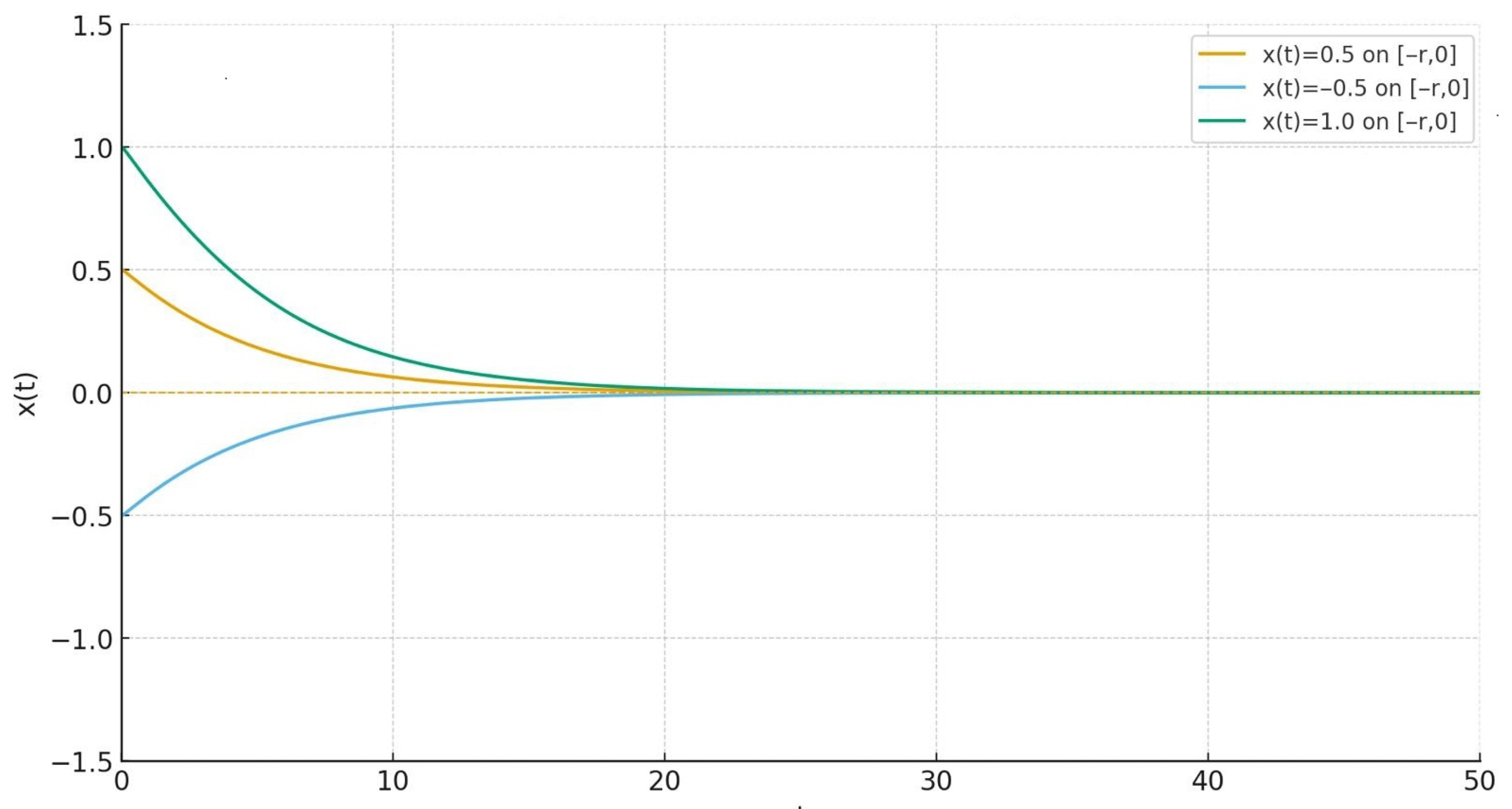
It can be shown that all hypotheses of Theorem 1 hold. As a result, it can be concluded that the solutions of (5) are asymptotically stable.

The following figure visualizes the asymptotic stability of the solutions of (5) by choosing $\alpha =1$ and $b_1=b_2=r_1=r_2=1$ to satisfy the condition $\alpha \ge \left({\displaystyle \frac{b_1+b_2}{19}}\right)$ given in Example 1 (Figure 1).

Example 2.

We examine the following nonlinear DDEs with two constant delays described by

$$x^{″}+\alpha (20x^{\prime }+sin{x}^{\prime })+{\displaystyle \frac{b_1}{r_1}}arctanx(t-r_1)+{\displaystyle \frac{b_2}{r_2}}arctanx(t-r_2)={\displaystyle \frac{x^{\prime }}{2(1+t^2+x^2)}}.$$

(7)

Equation (7) can be rewritten in its equivalent system as

$$x^{\prime }=y,$$

$$y^{\prime }=-\alpha (20y+siny)-{\displaystyle \frac{b_1}{r_1}}arctanx(t-r_1)-{\displaystyle \frac{b_2}{r_2}}arctanx(t-r_2)+{\displaystyle \frac{y}{2(1+t^2+x^2)}}.$$

(8)

In addition to the hypotheses of Theorem 1 shown in Example 1, when we compare (3) and (8),

$$p(t,x,y)={\displaystyle \frac{y}{2(1+t^2+x^2)}}$$

and the hypotheses of Theorem 2 hold for

$$p_0\left(t\right)={\displaystyle \frac{1}{1+t^2}}.$$

$$\underset{0}{\overset{\infty }{\int }}{p}_0\left(s\right)ds=\underset{0}{\overset{\infty }{\int }}{\displaystyle \frac{1}{1+s^2}}ds\le {\displaystyle \frac{\pi }{2}},$$

where $k={\displaystyle \frac{\pi }{2}}$.

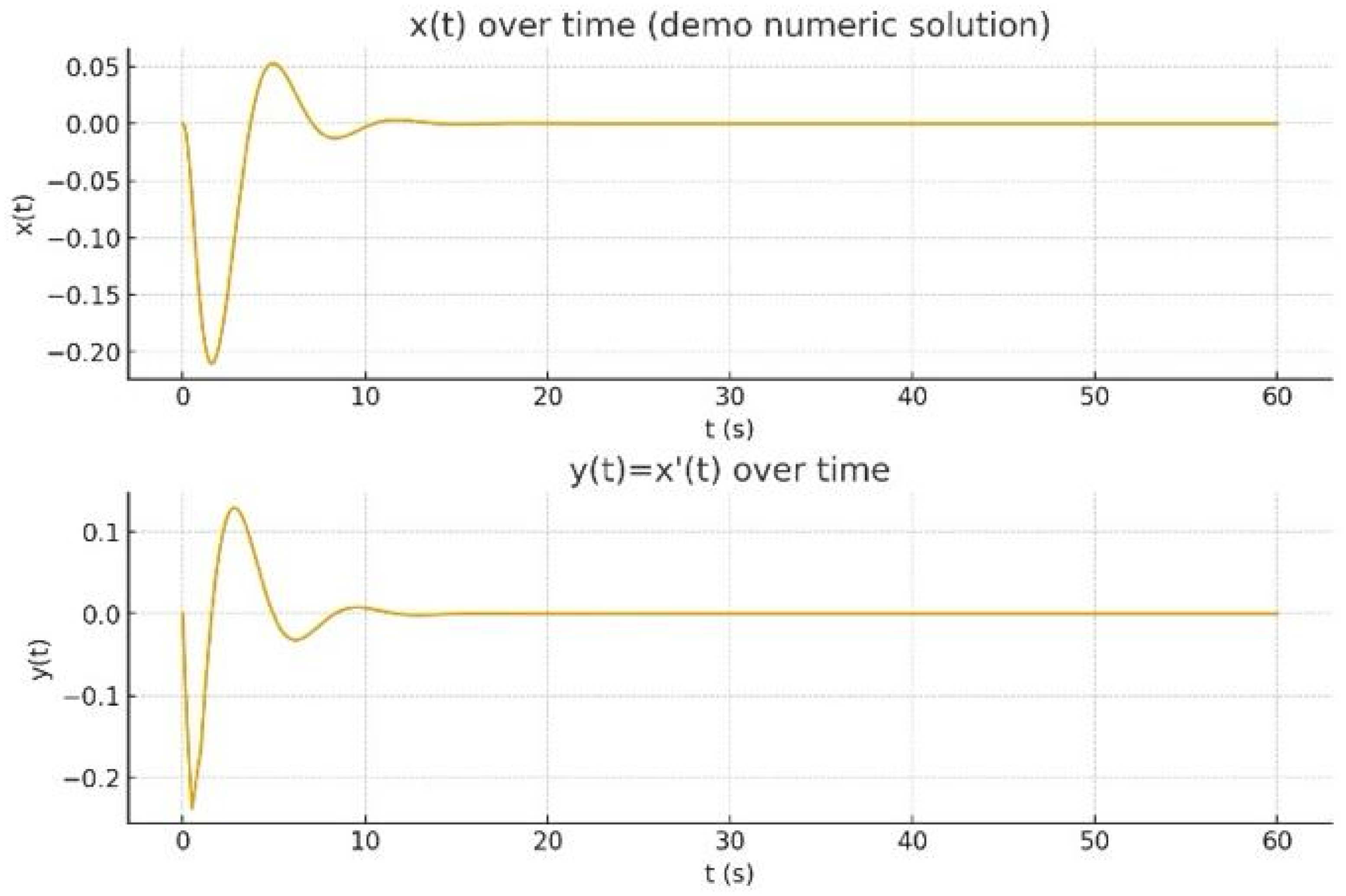
Since all the assumptions of Theorem 2 are fulfilled, the solutions of (6) are uniformly bounded (Figure 2).

2. Conclusions

In this study, we have investigated some qualitative behaviors of the solutions for a class of second-order nonlinear DDEs characterized by multiple constant delays. By employing appropriately constructed Lyapunov–Krasovskii functionals, we established new sufficient conditions that ensure the asymptotic stability, uniform boundedness, and square integrability of the solutions.

The results obtained in this study provide several significant refinements to the literature by generalizing the single-delay models found in [20,21,23] to multiple constant-delay configurations, which are more applicable to complex dynamical systems, and incorporating nonlinear perturbations $p(t,x,y)$ into the stability analysis. We demonstrated that the boundedness of solutions is intricately linked to the integrability of the perturbation function $p_0\left(t\right)$, a condition that we verified in Example 2. The examples and figures provided confirm that our theoretical criteria are not only mathematically rigorous but also practically applicable to nonlinear delayed systems, including sunflower-type equations.

Future research could extend these findings by considering time-varying delays or neutral-type differential structures, using the generalized framework established in this work as a foundational step.

References

1. Bellman, R. Stability Theory of Differential Equations; McGraw-Hill: New York, NY, USA, 1953. [Google Scholar]
2. Bihari, I. Researches on the boundedness and stability of the solutions of nonlinear differential equations. Acta Math. Acad. Sci. Hungar. 1957, 8, 261–278. [Google Scholar] [CrossRef]
3. Bhatia, N.P. Some oscillation theorems for second order differential equations. J. Math. Anal. Appl. 1966, 15, 442–446. [Google Scholar] [CrossRef]
4. Graef, J.R.; Spikes, P.W. Asymptotic behaviour of solutions of a second non-linear differential equation. J. Differ. Equ. 1975, 17, 461–476. [Google Scholar] [CrossRef]
5. Chang, S.H. Boundedness theorems for certain second order nonlinear differential equations. J. Math. Anal. Appl. 1970, 31, 509–516. [Google Scholar] [CrossRef][Green Version]
6. Zarghamee, M.S.; Mehri, B. A note on boundedness of solutions of certain second-order differential equations. J. Math. Anal. Appl. 1970, 31, 504–508. [Google Scholar] [CrossRef]
7. Burton, T.A. Stability and Periodic Solutions of Ordinary and Functional Differential Equations; Academic Press: Orlando, FL, USA, 1985. [Google Scholar]
8. Smith, H. An Introduction to Delay Differential Equations with Applications to the Life Sciences; Springer: New York, NY, USA, 2011. [Google Scholar]
9. Kolmanovskii, V.; Myshkis, A. Introduction to the Theory and Applications of Functional Differential Equations; Kluwer Academic Publishers: Dordrecht, The Netherlands, 1999. [Google Scholar]
10. Wu, M.; He, Y.; She, J.H. Stability Analysis and Robust Control of Time-Delay Systems; Springer: Berlin, Germany, 2010. [Google Scholar]
11. Tunç, C. Some new stability and boundedness results of solutions of Liénard type equations with a deviating argument. Nonlinear Anal. Hybrid Syst. 2010, 4, 85–91. [Google Scholar] [CrossRef]
12. Athanassov, Z.S. Boundedness criteria for solutions of certain second order nonlinear differential equations. J. Math. Anal. Appl. 1987, 123, 461–479. [Google Scholar] [CrossRef][Green Version]
13. Hatvani, L. On the stability of the zero solution of nonlinear second order differential equations. Acta Sci. Math. 1993, 57, 367–371. [Google Scholar]
14. Sugie, J.; Amano, Y. Global asymptotic stability of non-autonomous systems of Liénard type. J. Math. Anal. Appl. 2004, 289, 673–690. [Google Scholar] [CrossRef]
15. Tunç, C. On the boundedness of solutions of a non-autonomous differential equation of second order. Sarajevo J. Math. 2011, 7, 19–29. [Google Scholar] [CrossRef]
16. Tunç, C.; Tunç, O. On the boundedness and integration of non-oscillatory solutions of certain linear differential equations of second order. J. Adv. Res. 2016, 7, 165–168. [Google Scholar] [CrossRef][Green Version]
17. Tunç, C.; Tunç, E. On the asymptotic behavior of solutions of certain second-order differential equations. J. Frankl. Inst. 2007, 344, 391–398. [Google Scholar] [CrossRef]
18. Tunç, C.; Tunç, O. A note on the stability and boundedness of solutions to non-linear differential systems of second order. J. Assoc. Arab. Univ. Basic Appl. Sci. 2017, 24, 169–175. [Google Scholar] [CrossRef]
19. Gözen, M. New qualitative outcomes for ordinary differential systems of second order. Contemp. Math. 2023, 4, 1210–1221. [Google Scholar] [CrossRef]
20. Kulenović, M.R.S.; Ladas, G. Oscillations of the sunflower equation. Q. Appl. Math. 1988, 46, 23–28. [Google Scholar] [CrossRef][Green Version]
21. Lizana, M. Global analysis of the sunflower equation with small delay. Nonlinear Anal. Theory Methods Appl. 1999, 36, 697–706. [Google Scholar] [CrossRef]
22. Smirnova, V.B.; Proskurnikov, A.V.; Zgoda, I. The sunflower equation: Novel stability criteria. IFAC-PapersOnLine 2021, 54, 135–140. [Google Scholar] [CrossRef]
23. Abdurasid, A.A.; Aduloju, K.D.; Olutimo, A.L.; Omeike, M.O. Stability of solutions of the sunflower equation. Proyecciones J. Math. 2025, 44, 134–145. [Google Scholar] [CrossRef]
24. Adams, D.O.; Adeyanju, A.A.; Omeike, M.O. Asymptotic stability and boundedness criteria for a certain second order nonlinear differential equations. J. Niger. Math. Soc. 2024, 43, 81–88. [Google Scholar]
25. Adeyanju, A.A. Stability and boundedness criteria of solutions of a certain system of second order differential equations. Ann. Univ. Ferrara 2023, 69, 81–93. [Google Scholar] [CrossRef]
26. Gupta, D.; Bhalekar, S. Fractional order sunflower equation: Stability, bifurcation and chaos. Eur. Phys. J. Spec. Top. 2024, 234, 1595–1605. [Google Scholar] [CrossRef]
Figure 1. Solution of system of (6) for different three initial values.
Axioms 15 00067 g001
Figure 2. Bounded solution of system of (8) for different initial values.
Axioms 15 00067 g002
Disclaimer/Publisher’s Note: The statements, opinions and data contained in all publications are solely those of the individual author(s) and contributor(s) and not of MDPI and/or the editor(s). MDPI and/or the editor(s) disclaim responsibility for any injury to people or property resulting from any ideas, methods, instructions or products referred to in the content.