Partially Observed Two-Phase Point Processes

Abstract

In this paper, a two-phase spatio-temporal point process (STPP) defined on a countable metric space and characterized by a conditional intensity function is introduced. In the first phase, the process is memoryless, generating completely random point patterns. In the second phase, the location and occurrence time of each event depend on the spatial configuration of previous events, thereby inducing spatio-temporal correlation. Theoretical results that characterize the distributional properties of the process are established, enabling both efficient numerical simulation and Bayesian inference. A statistical inference framework is developed, for the setting in which the STPP is observed at discrete calendar dates while the spatial locations of events are recorded, their exact occurrence times are unobserved, i.e., interval-censored. This partial observation scheme commonly arises in ecological and epidemiological applications, such as the monitoring of plant disease or insect pest spread across a spatial grid over time. The methodology is illustrated through an analysis of the spatio-temporal spread of sugarcane yellow leaf virus (SCYLV) in an initially disease-free sugarcane plot in Guadeloupe, FrenchWest Indies.

1. Introduction

When studying a series of events distributed in time and space, spatio-temporal point process (STPP) theory provides powerful statistical modeling tools with important applications in many scientific areas [1,2,3,4]. Typical applications include earthquakes and disease outbreaks [5]. For example, ref. [6] developed a forecasting method for disease spread based on a non-stationary STPP. Ref. [7] presented major aspects of a particular class of STPPs by providing a review of spatio-temporal Hawkes point processes, focusing on simulation and estimation methods. Ref. [5] presented a review describing statistical models and methods for analyzing patterns of points in space and time, with emphasis on categories of observations or data collection. In many cases, the sampling effort is generally limited due to the spatial scale of observation. Thus, sampling procedures sometimes consist of recording the spatial location of new events between two consecutive sampling dates. Therefore, such an STPP is partially observed [8], as the event occurrence times are missing. In this paper, we investigate this kind of situation, which is of scientific interest. Due to the limited information on the STPP occurrence times, this model can be viewed as a marked point process observed at discrete dates [9], with both the counting process and the complete set of event marks recorded. One example is the study of the spatio-temporal spread of a viral infection in an experimental plot: an exhaustive census can be conducted on two consecutive dates to identify newly infected plants [10]. Because exact infection times are unobserved, standard likelihood-based methods for point processes that rely on conditional intensities [11,12,13] are inapplicable. However, data augmentation techniques [14,15] can leverage the resulting interval-censored observation scheme to enable valid statistical inference [16,17,18].

In this paper, we introduce a two-phase STPP in which spatial dependence emerges from a given date $\tau$, and we derive distributional results for this model that are useful for numerical simulations and statistical inference. The studied space is assumed to be countable. Section 2 presents the different notations used throughout the paper, along with basic definitions and motivating examples. The spatio-temporal model is introduced in Section 3, together with key distributional properties. Section 4 discusses data augmentation techniques for inference on the model parameters. Section 5 provides illustrations using data on the sugarcane yellow leaf virus (SCYLV), a vector-borne disease that can reduce sugarcane yields, increase production costs, and has been the subject of numerous studies over the past decade [19,20,21,22].

2. Notations, Basic Definitions and Examples

We consider a countable metric space $(X,d)$ and a filtered probability space ${\displaystyle (\Omega ,\mathcal{A},P,{\left({\mathcal{F}}_t\right)}_{t\in {\mathbb{R}}_{+}})}$. The filtration ${\displaystyle {\left({\mathcal{F}}_t\right)}_{t\in {\mathbb{R}}_{+}}}$ satisfies the usual conditions, in particular is right-continuous. X is a set of observable spatial units and ${\mathcal{F}}_t$ represents the history up to time t [11]. The history prior to time t is defined as ${\displaystyle {\mathcal{F}}_{t^{-}}=\bigcap _{u<t}{\mathcal{F}}_u}$.

A STPP on $X\times {\mathbb{R}}_{+}$ is a stochastic process whose realizations are point patterns in $X\times {\mathbb{R}}_{+}$. By point pattern, we mean a countable set of points. Each point represents the location and time of an event. It is useful for modeling patterns of events occurring over both space and time, such as disease outbreak cases, earthquakes, car accidents or crime incidents. An STPP on $X\times {\mathbb{R}}_{+}$ can be defined through a stochastic counting measure $N^{\ast }$ on $X\times {\mathbb{R}}_{+}$ [5,9]. For any subset B of $X\times {\mathbb{R}}_{+}$, the value $N^{\ast }\left(B\right)$ represents the number of points falling in B. The point process $N^{\ast }$ is simple if for any singleton B of $X\times {\mathbb{R}}_{+}$, we have $N^{\ast }\left(B\right)\in \{0,1\}$.

In the sequel, we use the following notations:

For any spatial unit x and time t, with $(x,t)$ in $X\times {\mathbb{R}}_{+}$, we denote by

$D_x$ the event time at site x,

$S_x\left(t\right)$ the state of site x at time t,

$S_x\left(t^{-}\right)$ the state of site x prior to time t,

$x_t$ the spatial location of the event which occurred at time t,

$I_t$ the subset of X where events occurred up to time t,

$I_t^{-}$ the subset of X where events occurred before time t,

$N_t$ the number of events up to time t.

Thus,

$$S_x\left(t\right)=\left\{\begin{array}{cc}1& \mathrm{if}{D}_x\le t\\ 0& \mathrm{if}{D}_x>t\end{array}\right.,S_x\left(t^{-}\right)=\left\{\begin{array}{cc}1& \mathrm{if}{D}_x<t\\ 0& \mathrm{if}{D}_x\ge t\end{array}\right.,$$

$$I_t=\{x\in X|S_x\left(t\right)=1\}=\{x\in X|D_x\le t\},I_t^{-}=\{x\in X|S_x\left(t^{-}\right)=1\}=\{x\in X|D_x<t\},$$

and

$$N_t=\sum _{x\in X}{S}_x\left(t\right).$$

The stochastic process ${\displaystyle N={\left(N_t\right)}_{t\in {\mathbb{R}}_{+}}}$ is the time counting process regardless of spatial location. Therefore, the STPP $N^{\ast }$ can be considered as a marked point process with event occurrences in ${\mathbb{R}}_{+}$ and marks in X. In [11] (Section 6.4), the authors refer to N as the ground process of $N^{\ast }$. Consequently, $N^{\ast }$ is simple if N is simple, and $N^{\ast }$ can be considered as a time point process with spatial marks in a countable space.

The point process conditional intensity at $(x,t)$ is denoted by ${\lambda }_x\left(t\right)$ and defined as follows:

$${\lambda }_x\left(t\right)=\underset{h\to 0^{+}}{lim}{\displaystyle \frac{1}{h}}P(D_x\in [t,t+h]|{\mathcal{F}}_{t^{-}})$$

which can also be expressed:

$${\lambda }_x\left(t\right)=\underset{h\to 0^{+}}{lim}{\displaystyle \frac{1}{h}}P(S_x(t+h)-S_x\left(t^{-}\right)=1|{\mathcal{F}}_{t^{-}}).$$

${\lambda }_x\left(t\right)$ represents the infinitesimal expected rate of events at time t and location x, given all the observations up to time t [3,23]. By specifying ${\lambda }_x\left(t\right)$ as in Equation (1), we provide a model for the STPP $N^{\ast }$.

The formalization introduced above is useful for studying the spatial–temporal progression of a virus epidemic in spatially located individuals, for example, plants in a crop field. In this case, X is the set of plant locations in the field, similar to a quasi-regular grid. $I_t$ is the set of infected plants at time t, and $S_x\left(t\right)$ is the infection state of plant located at x while $D_x$ is its infection date. $N_t$ is the number of infected plants up to time t. The infection risk for the plant located at x at time t is associated with ${\lambda }_x\left(t\right)$. Another example is the transmission of disease inside a set X of cattle farms in a region, similar to an irregular grid. $I_t$ is the set of test-positive farms at time t. The date for which farm x is first tested positive is $D_x$, and its state at time t is $S_x\left(t\right)$. The cumulative number of test-positive farms at time t is $N_t$. The risk for farm x to be test-positive at time t is associated with ${\lambda }_x\left(t\right)$. In each of these examples, there is an initial phase corresponding to the random introduction of the disease. Then comes a second phase during which the disease spreads mainly from one spatial unit to close neighbors. Studying how these events evolve over time within a countable set of spatial units is of scientific interest. It also involves addressing phenomena that have economic and health implications. Such a two-phase model is introduced in Section 3. The indicator function of any subset A of X is denoted by ${\mathbb{I}}_A$ and its cardinality by $♯A$.

3. The Model and Its Distributional Properties

We consider a two-phase model: in phase 1, the sequence of events is memoryless, while from a certain point in time, say $\tau$, phase 2 starts with interaction between events with respect to their spatial location. This STPP is specified by its conditional intensity function:

$$\forall (x,t)\in X\times {\mathbb{R}}_{+},{\lambda }_x\left(t\right)=\left\{\begin{array}{cc}{a}_{1}h\left(t\right){\mathbb{I}}_{[S_x\left(t^{-}\right)=0]}& \mathrm{if}t\le \tau \\ {\displaystyle \left(a_2+\sum _{y\in I_t^{-}}{f}_{\theta }\left(d(x,y)\right)\right)h\left(t\right){\mathbb{I}}_{[S_x\left(t^{-}\right)=0]}}& \mathrm{if}t>\tau \end{array}\right.$$

(1)

where $(\tau ,a_1,a_2)\in {\mathbb{R}}_{+}^3$, $\theta$ is a vector parameter of ${\mathbb{R}}^k$, and $f_{\theta }$ and h are non-negative functions with ${\displaystyle {\int }_0^{\infty }h\left(t\right)dt=1}$ for identifiability reasons [24,25]. Otherwise, $a_1$ and $a_2$ are identifiable only up to a multiplicative constant. Aspects of identifiability theory for parametric models can be found in [26].

The term ${\mathbb{I}}_{[S_x\left(t^{-}\right)=0]}$ implies that at most one event can occur in a given site x and time t. The parameters $a_1$ and $a_2$ represent the rescaled background intensities for each phase. External information about covariates is incorporated through the function h. This information is the same for any element x of X and varies only over time. Function $f_{\theta }$, hereafter referred to as the contact function, describes how the intensity at time t on site x varies with the distance between x and the spatial locations of events that occurred before t. This role is similar to that of the natural birth function in Hawkes branching point processes [27]. The process defined by (1) is a simple point process and is self-exciting only in the second phase when occurrences of events imply that other events are more likely to occur. Note that the interaction term in (1) has an integral form given by Equation (2):

$$\sum _{y\in I_t^{-}}{f}_{\theta }\left(d(x,y)\right)={\int }_{[0,t]}{f}_{\theta }\left(d(x,x_u)\right)dN\left(u\right)$$

(2)

Relevant distributional properties of the model are provided by Theorem 1:

Theorem 1.

For the STPP specified by expression (1), if X is a finite set of size n, then

(i) 

$\forall t\in [0,\tau ],N_t$ follows the binomial distribution ${\displaystyle \mathcal{B}\left(n,1-e^{-a_1{\int }_0^{t}h\left(u\right)du}\right)}$,

(ii) 

$\forall t\in [\tau ,+\infty ],$ conditionally to $N_t-N_{t^{-}}=1$, the event occurring at time t is localized at site x with probability:

$${\displaystyle \frac{{\displaystyle a_2+\sum _{y\in I_t^{-}}{f}_{\theta }\left(d(x,y)\right)}}{{\displaystyle a_2(n-N_{t^{-}})+\sum _{x\notin I_t^{-}}\sum _{y\in I_t^{-}}{f}_{\theta }\left(d(x,y)\right)}}}{\mathbb{I}}_{[x\notin I_t]}.$$

(iii) 

$\forall t\in [\tau ,+\infty ],$ conditional on ${\mathcal{F}}_t$, next event time $T_t$ on X from time t is distributed according to the following probability density $g_t$:

$$\forall v\in \mathbb{R},g_t\left(v\right)=K_{a_2,\theta }\left(t\right)h\left(v\right)exp\left(-K_{a_2,\theta }\left(t\right){\int }_t^{v}h\left(u\right)du\right){\mathbb{I}}_{[v>t]}$$

where ${\displaystyle K_{a_2,\theta }\left(t\right)=a_2(n-N_t)+\sum _{x\notin I_t}\sum _{y\in I_t}{f}_{\theta }\left(d(x,y)\right)}$.

Proof of Theorem 1.

(i) For $t\le \tau$, the process described by (1) is without memory so that the $S_x\left(t\right),x\in X,$ are independent and identically distributed according to a Bernoulli law. Therefore,

$$E\left(N_t\right)=E\left(\sum _{x\in X}{S}_x\left(t\right)\right)=\sum _{x\in X}P(D_x\le t)=n\left(1-exp(-{\int }_0^t{a}_{1}h\left(u\right)du)\right)$$

which completes the proof.

(ii)

For $t>\tau$ and $x\in X$, we have

$${\lambda }_x\left(t\right)=\left(a_2+\sum _{y\in I_t^{-}}{f}_{\theta }\left(d(x,y)\right)\right)h\left(t\right){\mathbb{I}}_{[x\notin I_t^{-}]}$$

(3)

so that the intensity of time process N conditional on ${\mathcal{F}}_{t^{-}}$ is

$$\begin{array}{cc}\hfill \sum _{x\in X}{\lambda }_x\left(t\right)=& {\displaystyle \sum _{x\in X}\left(a_2+\sum _{y\in I_t^{-}}{f}_{\theta }\left(d(x,y)\right)\right)h\left(t\right){\mathbb{I}}_{[x\notin I_t^{-}]}}\\ \hfill =& {\displaystyle \left(a_2(n-N_{t^{-}})+\sum _{x\notin I_t^{-}}\sum _{y\in I_t^{-}}{f}_{\theta }\left(d(x,y)\right)\right)h\left(t\right)}\end{array}$$

(4)

(3) and (4) lead us to the final result.

(iii)

For any v in $[t,T_t]$, we have $v\ge t>\tau$ so that Equation (4) leads to

$$\sum _{x\in X}{\lambda }_x\left(v\right)=\left(a_2(n-N_{v^{-}})+\sum _{x\notin I_v^{-}}\sum _{y\in I_v^{-}}{f}_{\theta }\left(d(x,y)\right)\right)h\left(v\right)=K_{a_2,\theta }\left(t\right)h\left(v\right)$$

because $N_{v^{-}}=N_t$ and $I_v^{-}=I_t$ since no event occurs in the interval $(t,v)$. The final result is easily derived from classical reliability theory.

   □

In the sequel, we refer to h as the external information function, and to $f_{\theta }$ as the contact function. There are several ways of modeling these two functions.

Table 1. Some examples of contact function $f_{\theta }$ for $X\subset {\mathbb{Z}}^2$, and the Euclidean metric d. The closed disk of center x and radius $\theta$ is denoted by $\mathcal{D}(x,\theta )$.

		Nearest Neighbor Influence
${\mathit{f}}_{\mathit{\theta }}\mathbf{\left(}\mathit{d}\mathbf{\right)}$	Interaction Term	$\mathit{\theta }\mathbf{=}\mathbf{1}$			$\mathit{\theta }\mathbf{=}\mathbf{2}$
	${\displaystyle \mathbf{\sum }_{\mathit{y}\mathbf{\in }{\mathit{I}}_{\mathit{t}}^{\mathbf{-}}}{\mathit{f}}_{\mathit{\theta }}\mathbf{\left(}\mathit{d}\mathbf{(}\mathit{x}\mathbf{,}\mathit{y}\mathbf{)}\mathbf{\right)}}$	$\mathit{d}\mathbf{=}\mathbf{1}$	$\mathit{d}\mathbf{=}\sqrt{\mathbf{2}}$	$\mathit{d}\mathbf{=}\mathbf{2}$	$\mathit{d}\mathbf{=}\mathbf{1}$	$\mathit{d}\mathbf{=}\sqrt{\mathbf{2}}$	$\mathit{d}\mathbf{=}\mathbf{2}$
0	0	0	0	0	0	0	0
${\theta }^{-1}$	${\theta }^{-1}{N}_{t^{-}}$	1	1	1	0.50	0.50	0.50
$e^{-\theta d}$	${\displaystyle \sum _{y\in I_t^{-}}{e}^{-\theta d(x,y)}}$	0.37	0.24	0.14	0.14	0.06	0.02
$d^{-2\theta }$	${\displaystyle \sum _{y\in I_t^{-}}d{(x,y)}^{-2\theta }}$	1	0.50	0.25	1	0.25	0.06
${(1+d)}^{-2\theta }$	${\displaystyle \sum _{y\in I_t^{-}}{(1+d(x,y))}^{-2\theta }}$	0.25	0.17	0.11	0.06	0.03	0.01
${\mathbb{I}}_{[0,\theta ]}\left(d\right)$	${\displaystyle ♯I_t^{-}\cap \mathcal{D}(x,\theta )}$	1	0	0	1	1	1

shows some numerical values for the interaction term associated with a single event located on a nearest neighbor of first, second or third order when X is a regular grid of ${\mathbb{Z}}^2$. For a given site x, the influence of neighbor y is quantified by means of $f_{\theta }\left(d(x,y)\right)$. For $f_{\theta }\equiv 0$, the conditional intensity does not take into account events prior to time t, and the model is without memory. For $f_{\theta }\ne 0$, the process N is Markovian. If $\theta \ne 0$ and $f_{\theta }\left(d\right)=e^{-\theta d}$ or $d^{-\theta }$, then the second phase of model (1) corresponds to models proposed by [8,16]. For $\theta >0$ and $f_{\theta }\left(d\right)={\mathbb{I}}_{[0,\theta ]}\left(d\right)$, the second phase of our model is a special case of the model presented by [18]. In what concerns the external information function h, ref. [18] used a normal density function for each observation date, whose parameters were estimated with external data. It is worth noticing that under mild conditions on h, there exists a time transformation which leads us to model (1) with $h\equiv 1$. In this paper, we consider that the external data available in a usable form are event count data. The external information is modeled here using a three-parameter Weibull distribution $\mathcal{W}(t_0,\beta ,\gamma )$:

$$\forall t\in {\mathbb{R}}_{+},h\left(t\right)={\displaystyle \frac{\gamma }{\beta }}{\left({\displaystyle \frac{t-t_0}{\beta }}\right)}^{(\gamma -1)}exp\left({\displaystyle -{\left(\frac{t-t_0}{\beta }\right)}^{\gamma }}\right){\mathbb{I}}_{[t_0,+\infty ]}\left(t\right).$$

(5)

The three parameters in (5) are all non-negative: the location parameter $t_0$ is the initial date from which the series of external events can be observed; $\beta$ is the scale parameter associated with a linear time transformation standardizing the expected external information to unity. Function h is bounded and unimodal if the shape parameter $\gamma$ is strictly greater than unity. Then, $\gamma$ is related to the date $t_M$ of maximal external information in the following way: ${\displaystyle t_M-t_0=\beta {\left(\frac{\gamma -1}{\gamma }\right)}^{\frac{1}{\gamma }}.}$ Therefore, for $\gamma \ge 1$, we have

$$\forall t\in {\mathbb{R}}_{+},h\left(t\right)\le h\left(t_M\right)\le {\displaystyle \frac{\gamma }{\beta }}.$$

(6)

In practice, $t_0$ is known, and statistical estimation concerns $\beta$ and $\gamma$.

4. Parameter Estimation

We assume that we have two sets of data. The first set consists of counts of external events at $n^{\prime }$ different dates ${\tau }_1\le \cdots \le {\tau }_{n^{\prime }}$. From this set, the estimates of the parameters $\beta$ and $\gamma$ in (5) can be obtained by using either least squares or maximum likelihood methods. For small $n^{\prime }$, the least squares estimation procedure over maximum likelihood is recommended by [28]. The second set consists of n maps describing the state of each site in X at successive dates $t_1\le \cdots \le t_n$:

$$\bigcup _{j=1}^n\{S_x\left(t_j\right),x\in X\}$$

(7)

from which we focus on inference about $\varphi =(a_1,a_2,\theta )$.

Let $t_1$ and $t_2$ be two observation dates such that $t_1<t_2$. Since the set of occurrence dates $\{D_{x_i},x_i\in I_{t_2}\setminus I_{t_1}\}$ is not observed, the inference techniques based on the STPP likelihood from the set of observations $\{(x_i,D_{x_i})x_i\in I_{t_2}\setminus I_{t_1}\}$ cannot be used [29]. An alternative method is importance sampling, but likelihood computation can be challenging [30].

Let us rewrite the conditional intensity given by expression (1) in a more general form:

$${\lambda }_x\left(t\right)=h\left(t\right)A_{\varphi }(x,I_{t^{-}})\times {\mathbb{I}}_{[S_x\left(t^{-}\right)=0]}$$

(8)

where $A_{\varphi }$ is a mapping from $\left(X,\mathcal{P}\left(X\right)\right)$ to ${\mathbb{R}}^{+}$ with $\mathcal{P}\left(X\right)$ denoting the power set of X.

The following Theorem 2 provides results that validate data completion with occurrence time imputations.

Theorem 2.

Let $Y=\{(x,D_x),x\in I_{t_2}\setminus I_{t_1}\}$ be the set of event locations and occurrence times over $(t_1,t_2]$. To be more explicit, let $k=N_{t_2}-N_{t_1}$ and $D_{x_0}=t_1$ so that ${\displaystyle Y=\{{(x_i,D_{x_i})}_{i\in [1,k]\cap \mathbb{N}},D_{x_{i-1}}<D_{x_i}\}}$.

(i) 

Denoting by $L(Y;\varphi )$ the log-likelihood of Y and ϕ for the model defined by (8), then conditional on $N_{t_2}-N_{t_1}=k$, we have

${\displaystyle L(Y;\varphi )=-\left(H\left(t_2\right)-H\left(D_{x_k}\right)\right)K_{\varphi }\left(D_{x_k}\right)}$

$$\begin{array}{c}\hfill +\sum _{i=1}^k\left(log(A_{\varphi }(x_i,I_{D_{x_i}^{-}}))+log\left(h\left(D_{x_i}\right)\right)-\left(H\left(D_{x_i}\right)-H\left(D_{x_{i-1}}\right)\right)K_{\varphi }\left(D_{x_{i-1}}\right)\right)\end{array}$$

(9)

where ${\displaystyle H\left(t\right)={\int }_0^{t}h\left(s\right)ds}$ and ${\displaystyle K_{\varphi }\left(t\right)=\sum _{x\in X}{A}_{\varphi }(x,I_t){\mathbb{I}}_{[S_x\left(t\right)=0]}}$.

(ii) 

Next event time $T_t$ on X from time t has a cumulative distribution function $F_{T_t}$ verifying

$$\forall v\in [t,+\infty ],F_{T_t}\left(v\right)=1-exp\left(-K_{\varphi }\left(t\right){\int }_t^{v}h\left(u\right)du\right).$$

Proof of Theorem 2.

(i) The log-likelihood (see [11], Section 7) for the STPP with conditional intensity given by (8) when observing Y is

$$L(Y;\varphi )=\sum _{i=1}^{k}log\left(A_{\varphi }(x_i,I_{D_{x_i}^{-}})h\left(D_{x_i}\right)\right)-\sum _{x\in X}{\int }_{t_1}^{t_2}h\left(u\right)A_{\varphi }(x,I_{u^{-}}){\mathbb{I}}_{[S_x\left(u^{-}\right)=0]}du.$$

(10)

The second term on the right side of Equation (10) is the negative integrated conditional intensity (compensator of point process N). By partitioning $[t_1,t_2]$ as follows:

$$t_1=D_{x_0}<D_{x_1}<\cdots <D_{x_k}<t_2=D_{x_{k+1}},$$

we get

$${\int }_{t_1}^{t_2}h\left(u\right)A_{\varphi }(x,I_{u^{-}}){\mathbb{I}}_{[S_x\left(u^{-}\right)=0]}du=\sum _{i=1}^{k+1}{\int }_{D_{x_{i-1}}}^{D_{x_i}}h\left(u\right)A_{\varphi }(x,I_{u^{-}}){\mathbb{I}}_{[S_x\left(u^{-}\right)=0]}du$$

$$=\sum _{i=1}^{k+1}{A}_{\varphi }(x,I_{D_{x_{i-1}}}){\mathbb{I}}_{[S_x\left(D_{x_{i-1}}\right)=0]}{\int }_{D_{x_{i-1}}}^{D_{x_i}}h\left(u\right)du$$

so that

$$\sum _{x\in X}{\int }_{t_1}^{t_2}h\left(u\right)A_{\varphi }(x,I_{u^{-}}){\mathbb{I}}_{[S_x\left(u^{-}\right)=0]}du=\sum _{i=1}^{k+1}\left(H\left(D_{x_i}\right)-H\left(D_{x_{i-1}}\right)\right)\sum _{x\in X}{A}_{\varphi }(x,I_{D_{x_{i-1}}}){\mathbb{I}}_{[S_x\left(D_{x_{i-1}}\right)=0]}$$

(ii)

According to (iii) in Theorem 1, the next event time $T_t$ on X from time t is distributed according to the following probability density:

$$K_{\varphi }\left(t\right)h\left(v\right)exp\left(-K_{\varphi }\left(t\right){\int }_t^{v}h\left(u\right)du\right){\mathbb{I}}_{[v>t]}$$

which leads to the final result.

   □

In our case, the set $y_2=\{D_x,x\in I_{t_2}\setminus I_{t_1}\}$ of occurrence times is not observed. Therefore, we have incomplete data, and expression (9) is not available.

Let $y_1=\{x\in I_{t_2}\setminus I_{t_1}\}$ be the incomplete data consisting of sites where events occurred. The posterior distribution of $\varphi$ can be obtained via data augmentation [14] by treating $y_2$ as a latent (unobserved) variable. Conditioning on the observed data $y_1$ and integrating over the missing data $y_2$ yields

$$\pi \left(\varphi \right|y_1)\propto \pi \left(\varphi \right)\int \pi \left(y_1\right|\varphi ,y_2)\pi \left(y_2\right|\varphi )d{y}_2.$$

The inference problem can be solved using Markov chain Monte Carlo (MCMC) methods [31,32,33], which generate samples from the full posterior distribution of $\varphi$ given $y_1$. These samples can then be used to approximate the posterior distribution and perform inference on parameters of interest. In particular, the MCMC output includes draws of the missing occurrence times, enabling imputation of plausible event dates to replace the unobserved ones. For further discussion of missing data imputation techniques in this context, see [34] for techniques on missing data imputation.

5. Application to the Sugarcane Yellow Leaf Virus Spread

5.1. Available Data

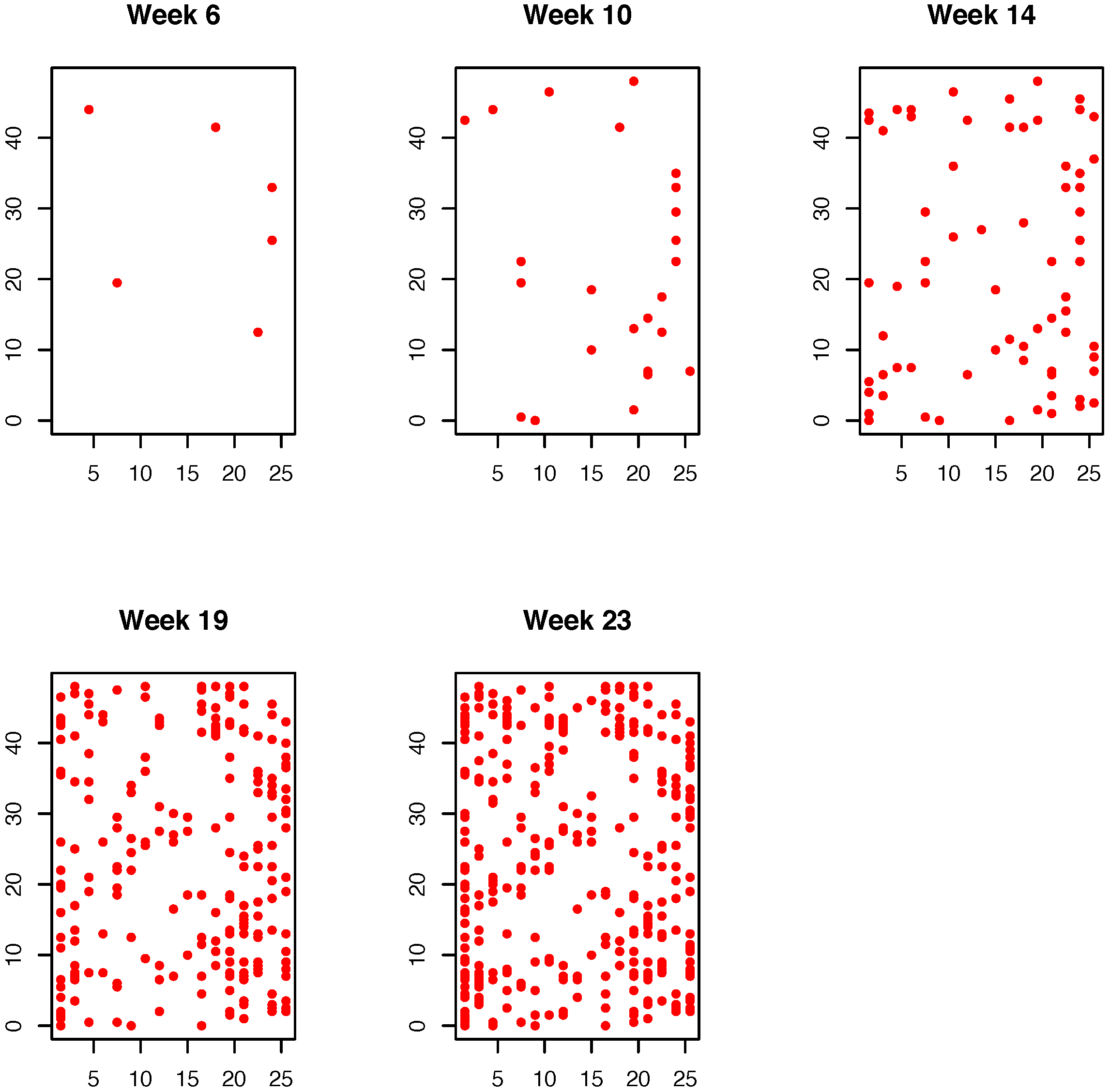
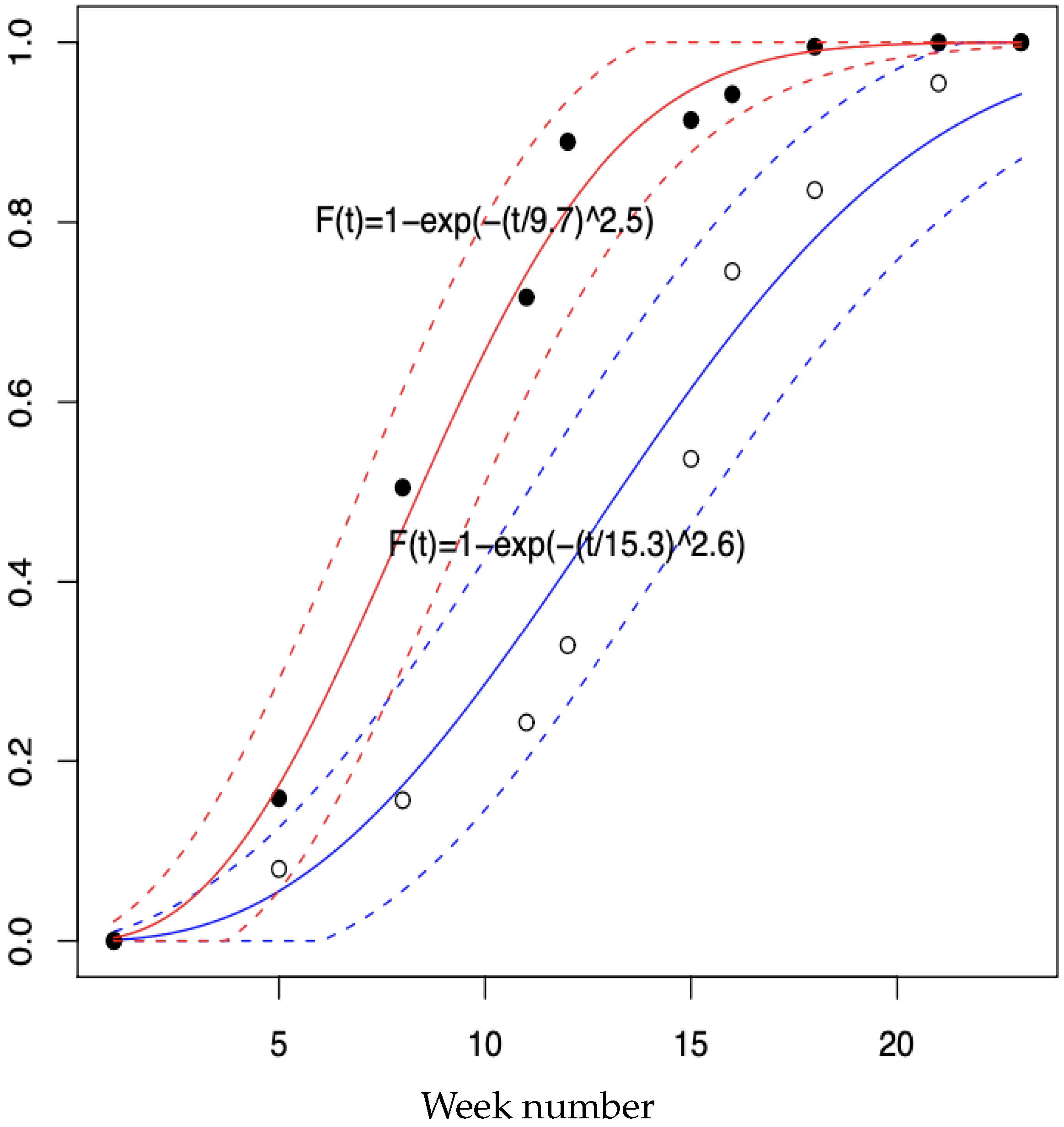
The inference method described above was applied to data collected from a sugarcane experimental field established at the CIRAD experimental station in Guadeloupe, French West Indies (F.W.I.). The observed plot comprised 1643 initially virus-free plants arranged in 17 rows with an inter-row spacing of 1.5 m. Each row contained approximately 95 plants, spaced 0.5 m apart. Data collection began five weeks after planting. The presence of sugarcane yellow leaf virus (SCYLV) was assessed for every plant in the plot using tissue blot immunoassay [35] at five observation dates: weeks 6, 10, 14, 19, and 23. Figure 1 displays the infection maps obtained at each of these dates. SCYLV is transmitted exclusively by aphids. In Guadeloupe, the primary vector is Melanaphis sacchari [22], whose population density was estimated via simple random sampling during weeks 5, 8, 11, 12, 15, 16, 18, 21, and 22 (Figure 2).

5.2. Spatio-Temporal Autocorrelation Index Tests

A criterion based on the number of newly infected neighbors was computed as a spatio-temporal generalization of the Moran index. To assess whether infections between two consecutive observation dates tended to occur in spatially proximate locations, we performed simulations based on random permutations of the plants newly infected during each interval. The results reveal strong and statistically significant positive spatio-temporal autocorrelation between weeks 14 and 19, as well as between weeks 19 and 23 (

Table 2. Spatio-temporal autocorrelation index (STI) and nullity test p-values.

Week 10		Week 14		Week 19		Week 23
STI	p -Value	STI	p -Value	STI	p -Value	STI	p -Value
−0.012	0.234	−0.024	0.720	0.117	0.000	0.071	0.001

). We note that [36] proposed a similar approach for analyzing time-series maps of diseased and healthy plants, including scenarios with missing plant data.

5.3. Fitting the Model to the Observed Data

The spread of insect-transmitted diseases is typically characterized by two components: first, infections originating from external inoculum sources outside the study region; and second, local within-region transmission [16,37,38].

The statistical analyses presented in Section 5.2 reveal two distinct phases in the contamination of the initially virus-free plot. The first phase is consistent with a complete random spatial pattern of infection. In the second phase, significant overdispersion and positive spatial autocorrelation in the number of infected plants are observed. These findings motivate the assessment of how well model (1) fits the observed data.

5.3.1. Phase 1

Let n denote the number of virus-free plants at date $t=0$. From Theorem 1, for $\tau >0$,

$$N_{\tau }\sim \mathcal{B}\left(n,1-e^{-a_{1}H\left(\tau \right)}\right)$$

and moment-based estimation yields a closed-form estimator $\widehat{a_1}$ of the background infection rate $a_1$:

$$\widehat{a_1}=-{\displaystyle \frac{1}{\widehat{H}\left(\tau \right)}}log\left(1-{\displaystyle \frac{N_{\tau }}{n}}\right)$$

where $\widehat{H}\left(\tau \right)$ is an estimate of the cumulative infective capacity at time $\tau$, given by

$$\widehat{H}\left(\tau \right)=1-exp\left({\displaystyle -{\left(\frac{\tau }{\widehat{\beta }}\right)}^{\widehat{\alpha }}}\right).$$

Here, $\widehat{\alpha }$ and $\widehat{\beta }$ are Weibull regression estimates obtained from the cumulative infective capacity of apterous adults and larvae of the aphid vector (Figure 2).

The phase change was assumed to occur at $\tau =14$. Using $\widehat{\beta }=15.3$ and $\widehat{\alpha }=2.6$, we obtain $\widehat{a_1}=0.077$.

5.3.2. Phase 2

The most widely used contact functions in the plant epidemiology literature are the exponential function which models rapid decay of infectivity with distance, and the inverse power function, which allows for non-negligible long-distance transmission, given, respectively, by Equations (12) and (11):

$$f_{\theta }\left(d\right)={(d+1)}^{-2\theta }$$

(11)

and

$$f_{\theta }\left(d\right)=exp(-\theta d).$$

(12)

In Guadeloupe, the transmissibility of SCYLV is maintained throughout the entire lifespan of aphids and is not lost even during their molting [22]. Consequently, for the second phase, we focus on estimating the parameter $\theta$ for both contact functions.

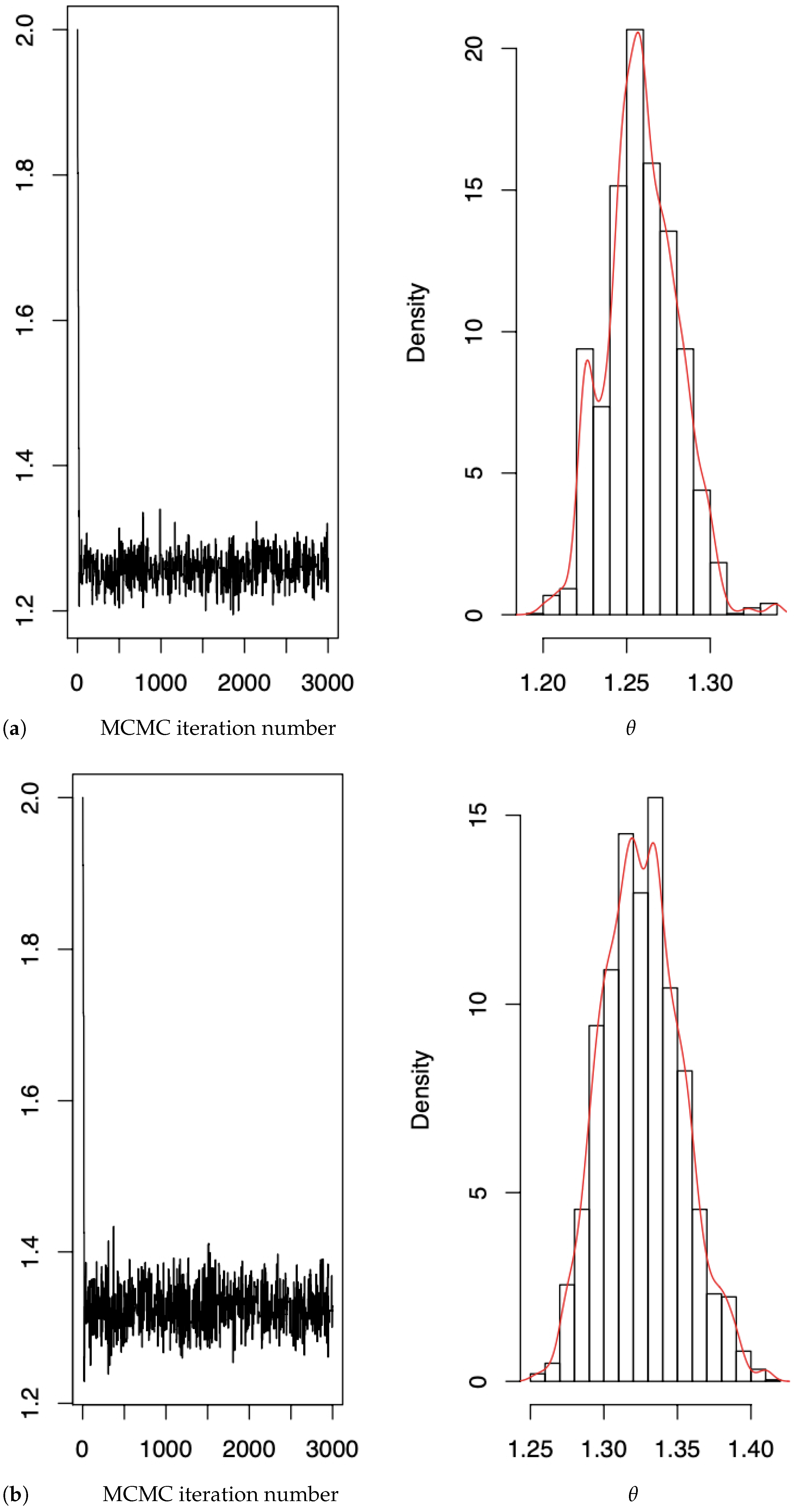
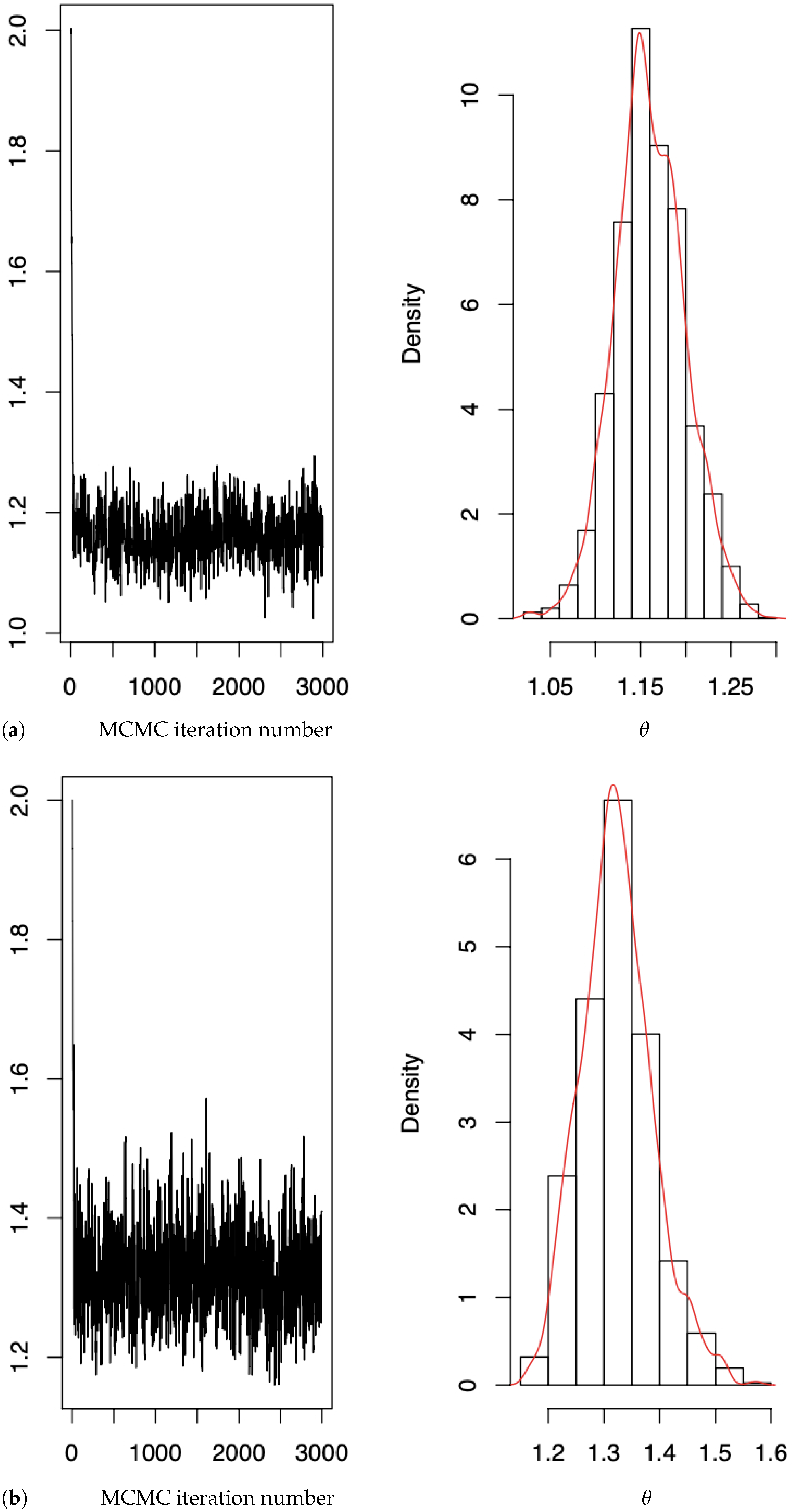
We denote by $\tilde{\theta }$ the posterior mean of $\theta$, and by $\widehat{\theta }$ its maximum a posteriori (MAP) estimator. Figure 3 and Figure 4 display the posterior distribution of $\theta$ obtained from the data observed between weeks 14 and 23. The 95% credible intervals for $\theta$ show no significant difference between the estimates based on the period from weeks 14 to 19 and those from weeks 19 to 23.

5.3.3. Validation of the Two-Phase Model

To assess the validity of our model, we conducted Monte Carlo goodness-of-fit tests following the framework of [39]. We computed five spatio-temporal summary statistics from the observed infection pattern:

(i)

The infected-to-healthy ratio (number of infected plants divided by the number of healthy plants);

(ii)

The dispersion index (variance-to-mean ratio of infection counts across spatial units);

(iii)

Moran’s spatial autocorrelation index for weeks 14–19 (see, e.g., Section 9.4 in [40]);

(iv)

Moran’s spatial autocorrelation index for weeks 19–23;

(v)

Extended Moran’s index for measuring spatio-temporal autocorrelation [41].

Each observed statistic was then compared to its empirical distribution under 1999 simulated realizations from the fitted model. The resulting Monte Carlo p-values are reported in

Table 3. Monte Carlo test p-values for the two contact functions.

Contact	Infected-to-	Dispersion	Moran Index	Moran Index	Extended Moran
Function	Healthy Ratio	Index	(Weeks 14–19)	(Weeks 19–23)	Index
Inverse power	0.138	0.251	0.274	0.13	0.108
Exponential	0.152	0.083	0.117	0.043	0.028

. The model based on the inverse power contact function (11) yields a consistently better fit than the exponential form (12): its simulated realizations more closely reproduce the observed values of spatio-temporal indices and the total number of infected plants. Although none of the p-values indicate perfect fit, those for the inverse power model are uniformly closer to the central range (e.g., 0.1–0.3), suggesting fewer systematic discrepancies. Overall, the inverse power model adequately captures the essential features of the epidemic spread. In particular, posterior predictive simulations using (11) successfully reproduce the observed spatial clustering of infected plants, supporting its use as a plausible representation of the underlying transmission process.

6. Conclusions

In this paper, we introduced a two-phase spatio-temporal point process (STPP) to model events distributed in time over a discrete spatial domain, accounting for limited temporal observation and latent event times. The first phase, characterized by a completely random distribution of events, is followed by a second phase of local, distance-dependent transmission governed by a spatial contact function. We established two theorems that provide key distributional properties of the model, facilitating data imputation and enabling statistical inference under partial observation of the STPP. Because event times are interval-censored (observed only at discrete calendar dates), standard likelihood inference based on conditional intensities is infeasible. We addressed this challenge via Bayesian data augmentation, treating unobserved event times as latent variables and sampling from the joint posterior distribution of the model parameters and event times using MCMC. This approach yields full posterior inference for the STPP parameters, as well as coherent imputations of the missing event time histories. We applied the framework to the spread of sugarcane yellow leaf virus (SCYLV) in an experimental sugarcane plot in Guadeloupe. Using Bayesian inference, we estimated the key parameters for two candidate contact functions (inverse power and exponential ones) and found that the inverse power law provides a superior fit to the observed spatio-temporal patterns. Posterior predictive checks confirm that the model accurately reproduces both the intensity and spatial clustering of infections in the field data. These results support the hypothesis that SCYLV transmission in Guadeloupe is driven primarily by short- to medium-range aphid movement, with non-negligible long-distance spread consistent with persistent virus retention in Melanaphis sacchari. The proposed framework offers a flexible and statistically principled methodology for analyzing partially observed spatio-temporal epidemic processes and is readily extensible to other vector-borne plant diseases under similar observation constraints.

References

1. Cheng, X.; Dong, Z.; Xie, Y. Deep Spatiotemporal Point Processes: Advances and New Directions. Annu. Rev. Stat. Its Appl. 2025, 13. [Google Scholar] [CrossRef]
2. Reinhart, A. A review of self-exciting spatio-temporal point processes and their applications. Stat. Sci. 2018, 33, 299–318. [Google Scholar]
3. Møller, J.; Ghorbani, M.; Rubak, E. Mechanistic spatio-temporal point process models for marked point processes, with a view to forest stand data. Biometrics 2016, 72, 687–696. [Google Scholar] [CrossRef]
4. Narayanan, S.; Kosmidis, I.; Dellaportas, P. Flexible marked spatio-temporal point processes with applications to event sequences from association football. J. R. Stat. Soc. Ser. C Appl. Stat. 2023, 72, 1095–1126. [Google Scholar] [CrossRef]
5. González, J.A.; Rodríguez-Cortés, F.J.; Cronie, O.; Mateu, J. Spatio-temporal point process statistics: A review. Spat. Stat. 2016, 18, 505–544. [Google Scholar] [CrossRef]
6. Dong, Z.; Zhu, S.; Xie, Y.; Mateu, J.; Rodríguez-Cortés, F.J. Non-stationary spatio-temporal point process modeling for high-resolution COVID-19 data. J. R. Stat. Soc. Ser. C Appl. Stat. 2023, 72, 368–386. [Google Scholar] [CrossRef]
7. Bernabeu, A.; Zhuang, J.; Mateu, J. Spatio-temporal hawkes point processes: A review. J. Agric. Biol. Environ. Stat. 2025, 30, 89–119. [Google Scholar] [CrossRef]
8. Gibson, G.; Austin, E. Fitting and testing spatio-temporal stochastic models with application in plant epidemiology. Plant Pathol. 1996, 45, 172–184. [Google Scholar] [CrossRef]
9. Andersen, P.K.; Borgan, O.; Gill, R.D.; Keiding, N. Statistical Models Based on Counting Processes; Springer Science & Business Media: Berlin, Germany, 2012. [Google Scholar]
10. Oscar, W.; Vaillant, J. Spatial Cluster Detection Under Dependent Random Environmental Effects. Mathematics 2025, 13, 430. [Google Scholar] [CrossRef]
11. Daley, D.J.; Vere-Jones, D. An Introduction to the Theory of Point Processes: Volume I: Elementary Theory and Methods; Springer: Berlin/Heidelberg, Germany, 2003. [Google Scholar]
12. Karr, A. Point Processes and Their Statistical Inference; Routledge: London, UK, 2017. [Google Scholar]
13. Kutoyants, Y.A. Efficient density estimation for ergodic diffusion processes. Stat. Inference Stoch. Process. 1998, 1, 131–155. [Google Scholar] [CrossRef]
14. Van Dyk, D.A.; Meng, X.L. The art of data augmentation. J. Comput. Graph. Stat. 2001, 10, 1–50. [Google Scholar] [CrossRef]
15. Yang, Y.; Longini, I.M., Jr.; Halloran, M.E. A data-augmentation method for infectious disease incidence data from close contact groups. Comput. Stat. Data Anal. 2007, 51, 6582–6595. [Google Scholar] [CrossRef]
16. Gibson, G.J. Markov chain Monte Carlo methods for fitting spatiotemporal stochastic models in plant epidemiology. J. R. Stat. Soc. Ser. C (Appl. Stat.) 1997, 46, 215–233. [Google Scholar]
17. Streftaris, G.; Gibson, G.J. Bayesian inference for stochastic epidemics in closed populations. Stat. Model. 2004, 4, 63–75. [Google Scholar] [CrossRef]
18. Rasmussen, J.G.; Møller, J.; Aukema, B.H.; Raffa, K.F.; Zhu, J. Continuous time modelling of dynamical spatial lattice data observed at sparsely distributed times. J. R. Stat. Soc. Ser. B Stat. Methodol. 2007, 69, 701–713. [Google Scholar] [CrossRef]
19. Rott, P.; Mirkov, T.E.; Schenck, S.; Girard, J.C. Recent advances in research on Sugarcane yellow leaf virus, the causal agent of sugarcane yellow leaf. Sugar Cane Int. 2008, 26, 18–22. [Google Scholar]
20. Daugrois, J.H.; Edon-Jock, C.; Bonoto, S.; Vaillant, J.; Rott, P. Spread of Sugarcane yellow leaf virus in initially disease-free sugarcane is linked to rainfall and host resistance in the humid tropical environment of Guadeloupe. Eur. J. Plant Pathol. 2011, 129, 71–80. [Google Scholar] [CrossRef]
21. Vaillant, J.; Puggioni, G.; Waller, L.A.; Daugrois, J. A spatio-temporal analysis of the spread of sugarcane yellow leaf virus. J. Time Ser. Anal. 2011, 32, 396–406. [Google Scholar] [CrossRef]
22. Holkar, S.K.; Balasubramaniam, P.; Kumar, A.; Kadirvel, N.; Shingote, P.R.; Chhabra, M.L.; Kumar, S.; Kumar, P.; Viswanathan, R.; Jain, R.K.; et al. Present status and future management strategies for Sugarcane yellow leaf virus: A major constraint to the global sugarcane production. Plant Pathol. J. 2020, 36, 536. [Google Scholar] [CrossRef]
23. Diggle, P.J. Statistical Analysis of Spatial and Spatio-Temporal Point Patterns; CRC Press: Boca Raton, FL, USA, 2013. [Google Scholar]
24. Walter, E. Identifiability of Parametric Models; Elsevier: Amsterdam, The Netherlands, 2014. [Google Scholar]
25. Chen, J.; Mu, W.; Li, Y.; Li, D. On the identifiability and interpretability of Gaussian process models. Adv. Neural Inf. Process. Syst. 2023, 36, 70267–70278. [Google Scholar]
26. Paulino, C.D.M.; de Bragança Pereira, C.A. On identifiability of parametric statistical models. J. Ital. Stat. Soc. 1994, 3, 125–151. [Google Scholar] [CrossRef]
27. Brémaud, P.; Massoulié, L. Hawkes branching point processes without ancestors. J. Appl. Probab. 2001, 38, 122–135. [Google Scholar] [CrossRef]
28. Hossain, A.; Howlader, H. Unweighted least squares estimation of Weibull parameters. J. Stat. Comput. Simul. 1996, 54, 265–271. [Google Scholar] [CrossRef]
29. Rathbun, S.L. Asymptotic properties of the maximum likelihood estimator for spatio-temporal point processes. J. Stat. Plan. Inference 1996, 51, 55–74. [Google Scholar] [CrossRef]
30. Marion, G.; Gibson, G.; Renshaw, E. Estimating likelihoods for spatio-temporal models using importance sampling. Stat. Comput. 2003, 13, 111–119. [Google Scholar] [CrossRef]
31. Robert, C.P. Mixtures of distributions: Inference and estimation. Markov Chain Monte Carlo Pract. 1996, 441, 464. [Google Scholar]
32. Robert, C.P.; Elvira, V.; Tawn, N.; Wu, C. Accelerating MCMC algorithms. Wiley Interdiscip. Rev. Comput. Stat. 2018, 10, e1435. [Google Scholar] [CrossRef]
33. Oscar, W.; Vaillant, J. Cox Processes Associated with Spatial Copula Observed through Stratified Sampling. Mathematics 2021, 9, 524. [Google Scholar] [CrossRef]
34. Neves, D.T.; Alves, J.; Naik, M.G.; Proença, A.J.; Prasser, F. From missing data imputation to data generation. J. Comput. Sci. 2022, 61, 101640. [Google Scholar] [CrossRef]
35. Schenck, S. Use of a tissue blot immunoassay to determine the distribution of Sugarcane yellow leaf virus in Hawaii. Sugar Cane 1997, 4, 5–8. [Google Scholar]
36. Thébaud, G.; Peyrard, N.; Dallot, S.; Calonnec, A.; Labonne, G. Investigating disease spread between two assessment dates with permutation tests on a lattice. Phytopathology 2005, 95, 1453–1461. [Google Scholar] [CrossRef] [PubMed]
37. Pethybridge, S.J.; Madden, L. Analysis of spatiotemporal dynamics of virus spread in an Australian hop garden by stochastic modeling. Plant Dis. 2003, 87, 56–62. [Google Scholar] [CrossRef]
38. Gottwald, T.; Gibson, G.; Garnsey, S.; Irey, M. Examination of the effect of aphid vector population composition on the spatial dynamics of citrus tristeza virus spread by stochastic modeling. Phytopathology 1999, 89, 603–608. [Google Scholar] [CrossRef][Green Version]
39. Baddeley, A.; Diggle, P.J.; Hardegen, A.; Lawrence, T.; Milne, R.K.; Nair, G. On tests of spatial pattern based on simulation envelopes. Ecol. Monogr. 2014, 84, 477–489. [Google Scholar] [CrossRef]
40. Bivand, R.S.; Pebesma, E.J.; Gomez-Rubio, V. Applied Spatial Data Analysis with R; Springer: Berlin/Heidelberg, Germany, 2008. [Google Scholar]
41. Gao, Y.; Cheng, J.; Meng, H.; Liu, Y. Measuring spatio-temporal autocorrelation in time series data of collective human mobility. Geo-Spat. Inf. Sci. 2019, 22, 166–173. [Google Scholar] [CrossRef]
Figure 1. Spatio-temporal spread of SCYLV in the observed plot.
Axioms 15 00059 g001
Figure 2. Cumulative infective capacity and its 95% confidence band for the alate aphids (red curves and black dots) and the apterous and larva aphids (blue curves and white dots).
Axioms 15 00059 g002
Figure 3. Sample path and posterior marginal distribution of θ for f θ ( d ) = ( d + 1 ) 2 θ : (a) t 1 = 14 , t 2 = 19 , θ ˜ = 1.26 , θ ^ = 1.25 ; 95% credible interval: [ 1.21 , 1.31 ] ; (b) t 1 = 19 , t 2 = 23 , θ ˜ = 1.34 , θ ^ = 1.33 ; 95% credible interval: [ 1.27 , 1.40 ] .
Axioms 15 00059 g003
Figure 4. Sample path and posterior marginal distribution of θ for f θ ( d ) = exp ( θ d ) : (a) t 1 = 14 , t 2 = 19 , θ ˜ = 1.16 , θ ^ = 1.15 ; 95% credible interval: [ 1.07 , 1.27 ] ; (b) t 1 = 19 , t 2 = 23 , θ ˜ = 1.32 , θ ^ = 1.33 ; 95% credible interval: [ 1.18 , 1.51 ] .
Axioms 15 00059 g004