Constraint Qualifications and Optimality Criteria for Nonsmooth Multiobjective Mathematical Programming Problems with Equilibrium Constraints on Hadamard Manifolds

Abstract

Nonsmooth multiobjective mathematical programming problems with equilibrium constraints (NMMPEC) are studied in this article in the Hadamard manifold setting. In the context of $\left(\mathrm{NMMPEC}\right)$, the generalized Guignard constraint qualification (GGCQ) is formulated within the framework of Hadamard manifolds. Moreover, Karush–Kuhn–Tucker (KKT)-type necessary optimality conditions are derived for $\left(\mathrm{NMMPEC}\right)$. Thereafter, we explore constraint qualifications (CQ) tailored to $\left(\mathrm{NMMPEC}\right)$ in the Hadamard manifold setting. Interrelations between these constraint qualifications are subsequently derived. It is further demonstrated that the proposed constraint qualifications, when satisfied, ensure that GGCQ holds. It is noteworthy that constraint qualifications and optimality conditions for $\left(\mathrm{NMMPEC}\right)$ have not been investigated in the Hadamard manifold setting.

1. Introduction

Mathematical programming problems with equilibrium constraints (MPEC) form a distinct subclass of constrained optimization models, distinguished by the presence of complementarity-type conditions or variational inequality constraints. An early contribution to the study of such optimization frameworks is the work of Harker and Pang [1], who established foundational existence results for efficient solutions to mathematical programs with equilibrium constraints (MPEC). Given their broad applicability across various domains of science, engineering, and technological systems (see, e.g., [2,3,4]), mathematical programs with equilibrium constraints (MPEC) have attracted substantial research interest in recent years. For a comprehensive discussion and recent developments on MPEC and their applications, the reader is referred to [5,6] and the references therein.

In recent decades, optimization problems formulated on manifolds has attracted substantial attention within the mathematical programming community, motivated by its strong theoretical foundations and extensive applicability (see, for example, [7,8] and the references therein). The setting of Euclidean geometry has been traditionally employed in data analysis in an extensive manner. In such a setting, the data points have been conveniently represented in terms of coordinates on the Euclidean space by several researchers (see, for instance, [9] and the references cited therein). In recent times, however, researchers have recognized the necessity of employing non-Euclidean geometry, specifically Riemannian geometry, to accurately represent data in more complex models (see, for instance, [9,10,11] and the references cited therein). Recasting classical optimization methods within a manifold framework not only broadens their scope but also introduces a number of fundamental advantages absent in the Euclidean setting. A wide class of constrained mathematical optimization problems on the Euclidean space admits reformulations into unconstrained models in the manifold framework, which often leads to a substantial reduction in the overall problem complexity; see [6,12] and the references therein. In addition, within the Riemannian geometric framework, several non-convex programming problems can be transformed into convex ones, see [13,14]. Motivated by these benefits, numerous fundamental notions of mathematical programming have been systematically generalized from Euclidean spaces to Riemannian and Hadamard manifolds in the existing literature; see, for example, [15,16,17,18,19] and the references cited therein.

It is noteworthy that nonsmooth phenomena frequently arise in real-world optimization problems across a wide range of applications (see, [20,21]). Classical nonsmooth optimization has been thoroughly investigated in the frameworks of both finite and infinite dimensional Banach spaces, where the underlying linear structure plays a fundamental role (see, [22,23]). In recent years, however, it has become increasingly evident that nonsmooth functions arise intrinsically on smooth manifolds across a broad range of contemporary research areas (see, [24,25]). To address nonsmooth optimization problems beyond the Euclidean framework, the concept of Clarke subdifferentials has been generalized to Riemannian manifolds, with particular emphasis on Hadamard manifolds (see, [26,27]). On Hadamard manifolds, the non-positive sectional curvature of the ambient space and the existence of unique geodesics ensure that Clarke subdifferentials are convex-valued, upper semicontinuous, making it a suitable tool for nonsmooth analysis on Hadamard manifolds (see, [8,26,27]). In view of this, in the present paper, the notion of Clarke subdifferentials have been employed to study NMMPEC on Hadamard manifolds.

The existing literature on mathematical programming problem with equilibrium constraints (MPEC) contain a wide range of regularity and optimality results. Foundational investigations into regularity conditions for MPEC were explored by Chen and Florian [28]. The Abadie constraint qualification for MPEC was subsequently examined by Flegel and Kanzow [29]. Optimality criteria for MPEC were further developed by Ye [30]. The generalized Guignard constraint qualification, together with associated optimality criteria, was analyzed by [31]. In the nonsmooth setting, optimality conditions for (MPEC) via convexificators were established by Ardali et al. [32]. Moreover, various duality models for (MPEC) with vector-valued objective function were derived by Singh and Mishra [5]. The notions of pseudonormality, local error bounds, and the Abadie constraint qualification for multiobjective $\left(\mathrm{MPEC}\right)$ were studied in Hejazi [33]. Pareto efficiency criteria and some constraint qualifications for smooth multiobjective (MPEC) were discussed by Zhang et al. [34].

Various optimality criteria for single-objective and multiobjective optimization problems (MOPs) involving differentiable functions, formulated on manifolds, have been investigated in a number of works (see, for reference, [18,35] and the references therein). In particular, classical constraint qualifications, including the linear independence, Mangasarian–Fromovitz, Abadie, and Guignard constraint qualifications have been studied for single-objective optimization problems on Riemannian manifolds by Bergmann and Herzog [35], while the Abadie constraint qualification has been explored for MOP in the Hadamard manifold setting by Tung and Tam [36]. Unlike Banach spaces, manifolds generally lack an inherent linear structure, which necessitates the development of alternative analytical tools when dealing with nonsmooth functions. This challenge has motivated growing interest in nonsmooth analysis on manifolds, as reflected in recent contributions such as [15,16,25,37]. Despite this progress, several important constraint qualifications, namely the Abadie, generalized Abadie, generalized Guignard, Mangasarian–Fromovitz, Cottle, and Slater conditions, along with corresponding optimality criteria for NMMPEC, have not yet been examined on Hadamard manifolds employing Clarke subdifferential calculus. The present work addresses this gap by formulating these constraint qualifications and deriving associated optimality conditions for NMMPEC on Hadamard manifolds using Clarke subdifferentials.

Motivated by the results established in [5,6,28,30], nonsmooth multiobjective programming problem with equilibrium constraints (NMMPEC) is explored in the present article, in the setting of Hadamard manifolds. We first formulate the generalized Guignard constraint qualification (GGCQ) for NMMPEC within the setting of Hadamard manifolds. Building on this, we derive necessary Pareto efficiency conditions for NMMPEC. We then introduce several constraint qualifications specifically adapted to the NMMPEC problem, namely, the Abadie, Cottle-type, Slater-type, and Mangasarian–Fromovitz-type conditions, in Hadamard manifold framework. Various relationships among these qualifications are established, and it is further shown that each serves as a sufficient condition for GGCQ. To illustrate the applicability and importance of the theoretical results, we include non-trivial examples on several Hadamard manifold models.

The distinguishing features and key contributions of this article may be outlined as follows. Firstly, motivated by the results derived by Maeda [22], within the framework of Hadamard manifolds, we develop a collection of constraint qualification concepts specifically adapted to $\left(\mathrm{NMMPEC}\right)$. It is noteworthy that constraint qualifications for NMMPEC have not been studied before in manifold setting using Clarke subdifferential. Secondly, the results obtained in this work extend the constraint qualifications introduced by Flegel and Kanzow [29,31] to the broader setting of Hadamard manifolds and to the more general class of problems, that is, NMMPEC. Furthermore, the optimality conditions derived in the present article generalize the corresponding results of Treanţă et al. [6] to the wider framework of nonsmooth multiobjective programs with equilibrium constraints.

The remainder of this article is structured as follows. Section 2 reviews the essential definitions and preliminary results needed for the analysis that follows. In Section 3, GGCQ for NMMPEC is presented on Hadamard manifolds, and KKT-type necessary conditions for NMMPEC are derived. In Section 4, we present several NMMPEC-adapt constraint qualifications and establish some interesting interrelations between them. In addition, it is demonstrated that the proposed constraint qualifications are sufficient to guarantee the validity of NMMPEC-GGCQ. Finally, in Section 5, we summarize the main contributions of the paper and outline several directions for future investigation.

2. Preliminaries

In this paper, ${\mathbb{R}}^n$ will signify the Euclidean n-space, while $\mathbb{N}$ stands for the set of natural numbers. The nonnegative orthant of ${\mathbb{R}}^n$, written as ${\mathbb{R}}_{+}^n$, is defined by

$${\mathbb{R}}_{+}^n:=\{(p_1,\dots ,p_n)\in {\mathbb{R}}^n:p_r\ge 0\mathrm{for}\mathrm{all}r=1,\dots ,n\}.$$

We use $\langle ·,·\rangle$ to refer to the usual inner product on ${\mathbb{R}}^n$. Let $y,z\in {\mathbb{R}}^n$. Then

$$\begin{array}{cc}\hfill y& \prec z⟺y_k<z_k,\forall k=1,2,\dots ,n.\hfill \\ \hfill y& ⪯z⟺y_k\le z_k,\forall k=1,2,\dots ,n.\hfill \end{array}$$

Let ${\mathbb{X}}^{\left(n\right)}$ denote an arbitrary Riemannian manifold of dimension n. The manifold ${\mathbb{X}}^{\left(n\right)}$ is called a Hadamard manifold if it is geodesically complete, simply connected, and has nonpositive sectional curvature everywhere. Hereafter, ${\mathbb{X}}^{\left(n\right)}$ will signify a Hadamard manifold of dimension n.

Let $\widehat{c}\in {\mathbb{X}}^{\left(n\right)}$. The tangent space at $\widehat{c}$ is signified by $T_{\widehat{c}}{\mathbb{X}}^{\left(n\right)}$. Notably, the exponential function ${\exp }_{\widehat{c}}:T_{\widehat{c}}{\mathbb{X}}^{\left(n\right)}\to {\mathbb{X}}^{\left(n\right)}$ is globally diffeomorphic. On the other hand, ${\exp }_{\widehat{c}}^{-1}:{\mathbb{X}}^{\left(n\right)}\to T_{\widehat{c}}{\mathbb{X}}^{\left(n\right)}$ satisfies ${\exp }_{\widehat{c}}^{-1}\left(\widehat{c}\right)=0$. Suppose that ${\widehat{c}}_1,{\widehat{c}}_2\in {\mathbb{X}}^{\left(n\right)}$. Then a unique minimal normalized geodesic ${\mathsf{\mu }}_{{\widehat{c}}_1,{\widehat{c}}_2}:[0,1]\to {\mathbb{X}}^{\left(n\right)}$ is guaranteed to exist for which ${\mathsf{\mu }}_{{\widehat{c}}_1,{\widehat{c}}_2}\left(s\right)={\exp }_{{\widehat{c}}_1}\left({s\exp }_{{\widehat{c}}_1}^{-1}\left({\widehat{c}}_2\right)\right),\forall s\in [0,1].$ It is important to note that ${\mathbb{X}}^{\left(n\right)}$ is diffeomorphic to ${\mathbb{R}}^n$. Let $\mathcal{W}:{\mathbb{X}}^{\left(n\right)}\to \mathbb{R}$ be a differentiable function. Then the gradient of $\mathcal{W}$, $grad\mathcal{W}$, is the vector field on ${\mathbb{X}}^{\left(n\right)}$, satisfying

$$d\mathcal{W}\left(X\right)=\langle grad\mathcal{W},X\rangle =X\left(\mathcal{W}\right),$$

for every vector field X on ${\mathbb{X}}^{\left(n\right)}$.

The definition stated below will be employed throughout the subsequent analysis; see [16].

Definition 1.

Let $\mathcal{Z}\subseteq {\mathbb{X}}^{\left(n\right)}$ and $\mathcal{W}:\mathcal{Z}\to \mathbb{R}$. The function $\mathcal{W}$ is called locally Lipschitz (l.l.) at $q\in \mathcal{Z}$ with rank $\mathcal{N}$ ($\mathcal{N}\in \mathbb{R}$, $\mathcal{N}>0$), provided for all $q_1,q_2$ belonging to some open neighborhood of q, such that

$$|\mathcal{W}\left(q_1\right)-\mathcal{W}\left(q_2\right)|\le K\omega (q_1,q_2),$$

where $\omega (q_1,q_2)$ is the Riemannian distance between $q_1$, $q_2\in \mathcal{Z}$.

$\mathcal{W}$ is called l.l. on $\mathcal{Z}$, provided it is l.l. at each point $z\in \mathcal{Z}$.

Remark 1.

It is worth emphasizing that certain functions which fail to satisfy the Lipschitz property in the Euclidean framework may possess this property when analyzed on Hadamard manifolds. To illustrate this phenomenon, consider the set $\mathcal{A}$ defined by

$$\mathcal{A}:=\{p=(p_1,p_2)\in {\mathbb{R}}^2:p_1>0,p_2>0\}.$$

Let $\mathcal{W}:\mathcal{A}\to \mathbb{R}$ be a real-valued mapping given by

$$\mathcal{W}\left(q\right)=\sum _{\mathfrak{s}=1}^{2}ln\left(q_{\mathfrak{s}}\right),$$

for every $q=\left(q_1,q_2\right)\in \mathcal{A}$. One observes that the function $\mathcal{W}$ fails to be Lipschitz on $\mathcal{A}$ with respect to the standard Euclidean structure. Nevertheless, the set $\mathcal{A}$ becomes a Hadamard manifold, say ${\mathcal{M}}_2$ once it is endowed with the Riemannian metric provided below:

$${\langle r,s\rangle }_q=\langle \mathcal{G}\left(q\right)r,s\rangle ,\forall r,s\in T_q\mathcal{A}={\mathbb{R}}^2,q\in \mathcal{A},$$

where

$$\mathcal{G}\left(q\right)=\left(\begin{array}{cc}{\displaystyle \frac{1}{q_1^2}}& 0\\ 0& {\displaystyle \frac{1}{q_2^2}}\end{array}\right).$$

It can then be shown that the function $\mathcal{W}$ possesses the Lipschitz property of rank 1 on ${\mathcal{M}}_2$ (see, [20]).

The definition given below can be found in [27].

Definition 2.

The set $\varnothing \ne \mathcal{D}(\subseteq {\mathbb{X}}^{\left(n\right)})$ is a geodesic convex, when for every $y,\tilde{y}\in \mathcal{D}$, there is a geodesic ${\gamma }_{y,\tilde{y}}:[0,1]\to {\mathbb{X}}^{\left(n\right)}$ connecting y and $\tilde{y}$. That is,

$${\gamma }_{y,\tilde{y}}\left(t\right)\in \mathcal{D},\forall t\in [0,1].$$

The definitions presented below are adapted from [37].

Definition 3.

The generalized directional derivative of a l.l. function $\mathcal{F}:{\mathbb{X}}^{\left(n\right)}\to \mathbb{R}$ at $q\in {\mathbb{X}}^{\left(n\right)}$ along $s\in T_q{\mathbb{X}}^{\left(n\right)}$ is given by

$${\mathcal{F}}^{\circ }(q;s):=\underset{p\to q,r\downarrow 0}{lim\; sup}{\displaystyle \frac{\mathcal{F}\left({exp}_{p}r{\left(d{exp}_q\right)}_{{exp}_q^{-1}p}s\right)-\mathcal{F}\left(p\right)}{r}},$$

where ${\left(d{exp}_q\right)}_{{exp}_q^{-1}p}:T_{{exp}_q^{-1}p}\left(T_q{\mathbb{X}}^{\left(n\right)}\right)\simeq T_q{\mathbb{X}}^{\left(n\right)}\to T_p{\mathbb{X}}^{\left(n\right)}$ is the differential of exponential map at ${exp}_q^{-1}p$.

Definition 4.

The Clarke subdifferential of a l.l. function $\mathcal{F}:{\mathbb{X}}^{\left(n\right)}\to \mathbb{R}$ at $p\in {\mathbb{X}}^{\left(n\right)}$ is given by

$${\partial }^c\mathcal{F}\left(p\right):=\left\{\mathsf{\zeta }\in T_p{\mathbb{X}}^{\left(n\right)}\mid {\mathcal{F}}^{\circ }(p;d)\ge \langle \mathsf{\zeta },d\rangle ,\forall d\in T_p{\mathbb{X}}^{\left(n\right)}\right\}.$$

The following result, adapted from [16], serves an important role in subsequent discussions.

Lemma 1.

Let $q\in {\mathbb{X}}^{\left(n\right)}$ and $\mathcal{F}:{\mathbb{X}}^{\left(n\right)}\to \mathbb{R}$ be a l.l. function with rank $\mathcal{L}$. Then

(a) 

${\partial }^c\mathcal{F}\left(q\right)$ is compact, convex, and nonempty. Moreover, $\parallel \mathsf{\zeta }\parallel \le \mathcal{L}$ for every $\mathsf{\zeta }\in {\partial }^c\mathcal{F}\left(q\right)$, and ${\partial }^c\mathcal{F}$ is upper semicontinuous at q.

(b) 

For every $s\in T_q{\mathbb{X}}^{\left(n\right)}$, the Clarke directional derivative satisfies

$${\mathcal{F}}^{\circ }(q;s)=max\{\langle \mathsf{\zeta },s\rangle :\mathsf{\zeta }\in {\partial }^c\mathcal{F}\left(q\right)\}.$$

(c) 

Let $\left\{q_n\right\}\subset {\mathbb{X}}^{\left(n\right)}$ and $\left\{{\mathsf{\zeta }}_n\right\}\subset T{\mathbb{X}}^{\left(n\right)}$ be sequences such that ${\mathsf{\zeta }}_n\in {\partial }^c\mathcal{F}\left(q_n\right)$ for all $n\in \mathbb{N}$ and $q_n\to q$. If $\mathsf{\zeta }$ is a cluster point of $\left\{{\mathcal{P}}_{q_n}^q{\mathsf{\zeta }}_n\right\}$, then $\mathsf{\zeta }\in {\partial }^c\mathcal{F}\left(q\right)$.

The lemma given below is from Grohs and Hosseini [25].

Lemma 2.

Let $\mathcal{F}:{\mathbb{X}}^{\left(n\right)}\to \mathbb{R}$ be a l.l. function. Let ${\mathcal{D}}_{\mathcal{W}}$ be the set consisting of every element where $\mathcal{F}$ exhibits differentiability on ${\mathbb{X}}^{\left(n\right)}$. Then

(i) 

${\mathcal{D}}_{\mathcal{F}}$ is dense in ${\mathbb{X}}^{\left(n\right)}$;

(ii) 

${\partial }^c\mathcal{F}\left(p\right)=co\left\{{lim}_{n\to \infty }grad\left(y_n\right):\left\{p_n\right\}\subseteq {\mathcal{D}}_{\mathcal{F}},y_n\to p\right\}.$

The subsequent definition is from Barani [37].

Definition 5.

Let $\mathcal{F}:\mathcal{D}\to \mathbb{R}$ be a l.l. function on a geodesic convex set $\mathcal{D}(\subseteq {\mathbb{X}}^{\left(n\right)})$. Then, $\mathcal{F}$ is geodesic convex at $\widehat{x}$, if for every $x\in \mathcal{D}$ and for every $\mathsf{\zeta }\in {\partial }^c\mathcal{F}\left(\widehat{x}\right)$, one has

$$\mathcal{F}\left(x\right)-\mathcal{F}\left(\widehat{x}\right)\ge {〈\mathsf{\zeta },{exp}_{\widehat{x}}^{-1}x〉}_{ \widehat{x}}.$$

(1)

$\mathcal{F}$ is called geodesic strictly convex at $\widehat{x}\in \mathcal{D}$, when the inequality in (1) holds strictly, with $\widehat{x}\ne x$. The function $\mathcal{F}$ is geodesic (strictly) concave at $\widehat{x}\in \mathcal{D}$, when $-\mathcal{F}$ is geodesic (strictly) convex at $\widehat{x}\in \mathcal{D}$. A function is geodesic affine at $\widehat{x}\in \mathcal{D}$ if it is both geodesically convex and geodesically concave at $\widehat{x}$.

Remark 2.

It is worth noting that many nonconvex functions in Euclidean spaces can become geodesically convex when viewed within an appropriate manifold framework. This allows a broader class of optimization problems to be analyzed by reformulating them on manifolds. For illustration, consider the set $\mathcal{D}\subset {\mathbb{R}}^2$ defined as follows:

$$\mathcal{D}:=\left\{y=\left(y_1,y_2\right)\in {\mathbb{R}}^2:y_2=y_1^2,y_1\in \left[{\displaystyle \frac{1}{2}},1\right]\right\}.$$

We consider $\mathcal{F}:\mathcal{D}\times \mathcal{D}\to \mathbb{R}$, as

$$\mathcal{F}(x,y)=y_1^2-y_1^4+y_2+y_2^2-x_1^2-x_2,x,y\in \mathcal{D},$$

$x=(x_1,x_2).$ By elementary calculations, one can verify that $\mathcal{D}$ is non-convex in ${\mathbb{R}}^2$.

• However, the set $\mathcal{D}$ may be regarded as the image of a geodesic segment on the paraboloid of revolution

  $$P(u_1,u_2)=\left(u_{2}cos{u}_1,u_{2}sin{u}_1,u_2^2\right),(u_1,u_2)\in \mathcal{D},$$

  when this surface is endowed with the Riemannian metric $\mathcal{G}$ defined by

  $$\mathcal{G}(u_1,u_2)=\left(\begin{array}{cc}{u}_2^2& 0\\ 0& 1+4u_2^2\end{array}\right).$$

Evidently, the set $\mathcal{D}$ is geodesic convex (see, for example, [38]). Moreover, although $\mathcal{F}(x,·)$ is not convex in the Euclidean setting, it becomes geodesically convex when restricted to the set $\mathcal{D}$.

The following theorem is from [37].

Theorem 1.

For any $x,y\in {\mathbb{X}}^{\left(n\right)}$ and a l.l. function $\mathcal{F}:{\mathbb{X}}^{\left(n\right)}\to \mathbb{R}$, some $t_0\in (0,1)$ and $z_0=\rho \left(t_0\right)$ exist, satisfying:

$$\mathcal{F}\left(y\right)-\mathcal{F}\left(x\right)\in 〈{\partial }^c\mathcal{F}\left(z_0\right),{\rho }^{\prime }\left(t_0\right)〉,$$

where $\rho \left(t\right):={exp}_x\left(t{exp}_x^{-1}\left(y\right)\right)$ and $t\in [0,1]$.

The subsequent lemma from [39] provides an extension of Motzkin’s theorem of the alternative in the context of Hadamard manifolds.

Lemma 3.

Fix a point $p\in {\mathbb{X}}^{\left(n\right)}$. Let $A\in {\mathbb{R}}^{m_1\times n}$, $B\in {\mathbb{R}}^{m_2\times n}$, and $C\in {\mathbb{R}}^{m_3\times n}$ be matrices whose rows belong to the tangent space at p. More precisely, $A_{\mathfrak{s}}\in T_p{\mathbb{X}}^{\left(n\right)}$ for $\mathfrak{s}=1,\dots ,m_1$, $B_{\mathfrak{p}}\in T_p{\mathbb{X}}^{\left(n\right)}$ for $\mathfrak{p}=1,\dots ,m_2$, and $C_k\in T_p{\mathbb{X}}^{\left(n\right)}$ for $k=1,\dots ,m_3$. Under these conditions, exactly one of the following statements holds, and they cannot occur simultaneously.

(a) 

The system of inequalities

$$\begin{array}{cccc}\hfill {\langle A_{\mathfrak{s}},x\rangle }_p& <0,\hfill & \hfill & \forall \mathfrak{s}=1,2,\dots ,m_1,\hfill \\ \hfill {\langle B_{\mathfrak{p}},x\rangle }_p& \le 0,\hfill & \hfill & \forall \mathfrak{p}=1,2,\dots ,m_2,\hfill \\ \hfill {\langle C_k,x\rangle }_p& =0,\hfill & \hfill & \forall k=1,2,\dots ,m_3,\hfill \end{array}$$

has a solution $x\in T_p{\mathbb{X}}^{\left(n\right)}$;

(b) 

The following equation

$$A^T{z}_1+B^T{z}_2+c^T{z}_3=0,$$

has a solution $z_1\in {\mathbb{R}}^{m_1}$, $z_2\in {\mathbb{R}}^{m_2}$, $z_3\in {\mathbb{R}}^{m_3}$, such that $z_1\ge 0$, $z_2\geqq 0$.

For an in-depth treatment of Riemannian manifolds and their role in optimization, the reader is referred to [23,27,40,41,42].

3. Optimality Criteria for NMMPEC

Throughout the remainder of this paper, the subsequent $\left(\mathrm{NMMPEC}\right)$ will be examined:

$$\begin{array}{c}\hfill \left(\mathrm{NMMPEC}\right)\mathrm{Minimize}\mathcal{F}\left(y\right):=\left({\mathcal{F}}_1\left(y\right),{\mathcal{F}}_2\left(y\right),\dots ,{\mathcal{F}}_r\left(y\right)\right)\end{array}$$

$$\begin{array}{cccc}\hfill \mathrm{subject}\mathrm{to}{\mathcal{W}}_{\mathfrak{p}}\left(y\right)& \le 0,\hfill & \hfill & \forall \mathfrak{p}\in {\mathcal{I}}^{\mathcal{W}}:=\{1,2,\dots ,t\},\hfill \\ \hfill {\mathcal{V}}_{\mathfrak{p}}\left(y\right)& =0,\hfill & \hfill & \forall \mathfrak{p}\in {\mathcal{I}}^{\mathcal{V}}:=\{1,2,\dots ,p\},\hfill \\ \hfill {\mathcal{C}}_{\mathfrak{p}}\left(y\right)& \ge 0,\hfill & \hfill & \forall \mathfrak{p}\in \mathcal{T}:=\{1,2,\dots ,m\},\hfill \\ \hfill {\mathcal{D}}_{\mathfrak{p}}\left(y\right)& \ge 0,\hfill & \hfill & \forall \mathfrak{p}\in \mathcal{T},\hfill \\ \hfill {\mathcal{D}}_{\mathfrak{p}}\left(y\right){\mathcal{C}}_{\mathfrak{p}}\left(y\right)& =0,\hfill & \hfill & \forall \mathfrak{p}\in \mathcal{T},\hfill \end{array}$$

where ${\mathcal{F}}_{\mathfrak{p}}:{\mathbb{X}}^{\left(n\right)}\to \mathbb{R}$ ($\mathfrak{p}\in \mathcal{I}:=\{1,2,\dots ,r\})$, ${\mathcal{W}}_{\mathfrak{p}}:{\mathbb{X}}^{\left(n\right)}\to \mathbb{R}$, ($\mathfrak{p}\in {\mathcal{I}}^{\mathcal{W}}$), ${\mathcal{V}}_{\mathfrak{p}}:{\mathbb{X}}^{\left(n\right)}\to \mathbb{R}$ ($\mathfrak{p}\in {\mathcal{I}}^{\mathcal{V}}$), ${\mathcal{C}}_{\mathfrak{p}}:{\mathbb{X}}^{\left(n\right)}\to \mathbb{R}$, ${\mathcal{D}}_{\mathfrak{p}}:{\mathbb{X}}^{\left(n\right)}\to \mathbb{R}$ ($\mathfrak{p}\in \mathcal{T}$) are l.l. on ${\mathbb{X}}^{\left(n\right)}$.

Let $\mathcal{S}$ refer the feasible set of NMMPEC. The next definitions recall the solution concept of NMMPEC (see, [22]).

Definition 6.

A point $\widehat{p}\in \mathcal{S}$ is Pareto efficient solution of NMMPEC, provided no other $\tilde{p}\in \mathcal{S}$ exists, satisfying

$$\begin{array}{cc}\hfill \mathcal{F}\left(\tilde{p}\right)& ⪯\mathcal{F}\left(\widehat{p}\right)\mathit{with}\mathcal{F}\left(\tilde{p}\right)\ne \mathcal{F}\left(\widehat{p}\right).\hfill \end{array}$$

Definition 7.

A point $\widehat{p}\in \mathcal{S}$ is weak Pareto efficient solution of NMMPEC, provided no other $\tilde{p}\in \mathcal{S}$ exists, satisfying

$$\begin{array}{cc}\hfill \mathcal{F}\left(\tilde{p}\right)& \prec \mathcal{F}\left(\widehat{p}\right).\hfill \end{array}$$

Hereafter, we will use $\mathcal{P}\left(S\right)$ to refer the collection of Pareto efficient solutions of NMMPEC.

Let $\widehat{q}\in \mathcal{S}$. We define

$$\begin{array}{cc}\hfill {\mathcal{A}}^{\mathcal{W}}\left(\widehat{q}\right)& :=\{\mathfrak{p}\in {\mathcal{I}}^{\mathcal{W}}:{\mathcal{W}}_{\mathfrak{p}}\left(\widehat{q}\right)=0\},\hfill \\ \hfill {\mathcal{E}}_{+0}\left(\widehat{q}\right)& :=\left\{\mathfrak{p}\in \mathcal{T}:{\mathcal{C}}_{\mathfrak{p}}\left(\widehat{q}\right)>0,{\mathcal{D}}_{\mathfrak{p}}\left(\widehat{q}\right)=0\right\},\hfill \\ \hfill {\mathcal{E}}_{0+}\left(\widehat{q}\right)& :=\left\{\mathfrak{p}\in \mathcal{T}:{\mathcal{C}}_{\mathfrak{p}}\left(\widehat{q}\right)=0,{\mathcal{D}}_{\mathfrak{p}}\left(\widehat{q}\right)>0\right\},\hfill \\ \hfill {\mathcal{E}}_{00}\left(\widehat{q}\right)& :=\left\{\mathfrak{p}\in \mathcal{T}:{\mathcal{C}}_{\mathfrak{p}}\left(\widehat{q}\right)=0,{\mathcal{D}}_{\mathfrak{p}}\left(\widehat{q}\right)=0\right\}.\hfill \end{array}$$

Remark 3.

(a) 

The index set ${\mathcal{E}}_{00}\left(\widehat{q}\right)$ is called the degenerate index set at $\widehat{q}$.

(b) 

It should be emphasized that the index sets defined above are determined by the particular choice of $\widehat{q}\in \mathcal{S}$. However, for the remainder of the paper, this dependence will be left implicit whenever it is clear from the context.

Let $\tilde{y}\in \mathcal{S}$ and $k\in \mathcal{I}$. Consider ${\mathcal{L}}^k$ and $\mathcal{L}$, defined below:

$$\begin{array}{cc}\hfill {\mathcal{L}}^k& :=\left\{y\in \mathcal{S}:{\mathcal{F}}_{\mathfrak{p}}\left(y\right)\le {\mathcal{F}}_{\mathfrak{p}}\left(\tilde{y}\right),\forall \mathfrak{p}\in \mathcal{I},\mathfrak{p}\ne k\right\},\hfill \\ \hfill \mathcal{L}& :=\left\{y\in \mathcal{S}:{\mathcal{F}}_{\mathfrak{p}}\left(y\right)\le {\mathcal{F}}_{\mathfrak{p}}\left(\tilde{y}\right),\forall \mathfrak{p}\in \mathcal{I}\right\}.\hfill \end{array}$$

Remark 4.

The following relation evidently follows from the above definitions:

$$\bigcap _{k\in \mathcal{I}}{\mathcal{L}}^k=\mathcal{L}.$$

The subsequent definition is from [43].

Definition 8.

Let $\mathcal{D}\subseteq {\mathbb{X}}^{\left(n\right)}$ and $\tilde{\mathit{\kappa }}$ be any point in the closure of $\mathcal{D}$. The Bouligand tangent cone of $\mathcal{D}$ at $\tilde{\mathit{\kappa }}$, is defined as

$$\begin{array}{cc}\hfill {\mathcal{C}}^{Tan}(\mathcal{D},\tilde{\mathit{\kappa }}):=\{\widehat{s}\in T_{\tilde{\mathit{\kappa }}}{\mathbb{X}}^{\left(n\right)}:\exists l_n\downarrow 0,\exists {\left\{{\widehat{s}}_n\right\}}_{n=1}^{\infty }& \subset T_{\tilde{\mathit{\kappa }}}{\mathbb{X}}^{\left(n\right)},{\widehat{s}}_n\to \widehat{s},\hfill \\ & {exp}_{\tilde{\mathit{\kappa }}}\left(l_n{\widehat{s}}_n\right)\in \mathcal{D},\forall n\in \mathbb{N}\}.\hfill \end{array}$$

Below, we define the notion of NMMPEC-adapt linearizing cone in manifold setting using Clarke subdifferential.

Definition 9.

Let $\tilde{\mathit{\kappa }}\in \mathcal{S}$ be arbitrary. The NMMPEC-adapt linearizing cone to $\mathcal{L}$ at $\tilde{\mathit{\kappa }}$ is defined below:

$$\begin{array}{cccccc}\hfill {\mathcal{C}}_{MMPEC}^{Lin}\left(\mathcal{L},\tilde{\mathit{\kappa }}\right):=\{\overline{u}\in T_{\tilde{\mathit{\kappa }}}{\mathbb{X}}^{\left(n\right)}:& \langle {\mathsf{\zeta }}_{\mathfrak{p}}^{\mathcal{F}},\overline{u}\rangle \hfill & \hfill & \le 0,\hfill & \hfill & \forall {\mathsf{\zeta }}_{\mathfrak{p}}^{\mathcal{F}}\in {\partial }^c{\mathcal{F}}_{\mathfrak{p}}\left(\tilde{\mathit{\kappa }}\right),\forall \mathfrak{p}\in \mathcal{I},\hfill \\ \hfill & \langle {\mathsf{\zeta }}_{\mathfrak{p}}^{\mathcal{W}},\overline{u}\rangle \hfill & \hfill & \le 0,\hfill & \hfill & \forall {\mathsf{\zeta }}_{\mathfrak{p}}^{\mathcal{W}}\in {\partial }^c{\mathcal{W}}_{\mathfrak{p}}\left(\tilde{\mathit{\kappa }}\right),\forall \mathfrak{p}\in {\mathcal{A}}^{\mathcal{W}},\hfill \\ \hfill & \langle {\mathsf{\zeta }}_{\mathfrak{p}}^{\mathcal{V}},\overline{u}\rangle \hfill & \hfill & =0,\hfill & \hfill & \forall {\mathsf{\zeta }}_{\mathfrak{p}}^{\mathcal{V}}\in {\partial }^c{\mathcal{V}}_{\mathfrak{p}}\left(\tilde{\mathit{\kappa }}\right),\forall \mathfrak{p}\in {\mathcal{I}}^{\mathcal{V}},\hfill \\ \hfill & \langle {\mathsf{\zeta }}_{\mathfrak{p}}^{\mathcal{C}},\overline{u}\rangle \hfill & \hfill & =0,\hfill & \hfill & \forall {\mathsf{\zeta }}_{\mathfrak{p}}^{\mathcal{C}}\in {\partial }^c{\mathcal{C}}_{\mathfrak{p}}\left(\tilde{\mathit{\kappa }}\right),\forall \mathfrak{p}\in {\mathcal{E}}_{0+},\hfill \\ \hfill & \langle {\mathsf{\zeta }}_{\mathfrak{p}}^{\mathcal{D}},\overline{u}\rangle \hfill & \hfill & =0,\hfill & \hfill & \forall {\mathsf{\zeta }}_{\mathfrak{p}}^{\mathcal{D}}\in {\partial }^c{\mathcal{D}}_{\mathfrak{p}}\left(\tilde{\mathit{\kappa }}\right),\forall \mathfrak{p}\in {\mathcal{E}}_{+0},\hfill \\ \hfill & \langle {\mathsf{\zeta }}_{\mathfrak{p}}^{\mathcal{C}},\overline{u}\rangle \hfill & \hfill & \ge 0,\hfill & \hfill & \forall {\mathsf{\zeta }}_{\mathfrak{p}}^{\mathcal{C}}\in {\partial }^c{\mathcal{C}}_{\mathfrak{p}}\left(\tilde{\mathit{\kappa }}\right),\forall \mathfrak{p}\in {\mathcal{E}}_{00},\hfill \\ \hfill & \langle {\mathsf{\zeta }}_{\mathfrak{p}}^{\mathcal{D}},\overline{u}\rangle \hfill & \hfill & \ge 0,\hfill & \hfill & \forall {\mathsf{\zeta }}_{\mathfrak{p}}^{\mathcal{D}}\in {\partial }^c{\mathcal{D}}_{\mathfrak{p}}\left(\tilde{\mathit{\kappa }}\right),\forall \mathfrak{p}\in {\mathcal{E}}_{00}\}.\hfill \end{array}$$

Remark 5.

(a) 

Definition 9 extends Definition 3.1 of Maeda [22] from the Euclidean setting to that of Hadamard manifolds. In addition, Definition 9 generalizes Definition 3.1 in Maeda [22] to the class of NMMPEC.

(b) 

When ${\mathbb{X}}^{\left(n\right)}={\mathbb{R}}^n$, Definition 9 extends the linearizing cone notion introduced by Singh and Mishra [5] for NMMPEC.

To derive KKT-type necessary optimality criteria for NMMPEC, we now define NMMPEC-adapt GGCQ on Hadamard manifolds for NMMPEC.

Definition 10.

Let $\overline{q}\in \mathcal{S}$. The NMMPEC-adapt generalized Guignard constraint qualification (NMMPEC-GGCQ) satisfies at $\overline{q}$, when

$${\mathcal{C}}_{NMMPEC}^{Lin}\left(\mathcal{L},\overline{q}\right)\subseteq \bigcap _{\mathfrak{p}\in \mathcal{I}}clco{\mathcal{C}}^{Tan}\left({\mathcal{L}}^j,\overline{q}\right).$$

The lemma below is employed in the derivation of the principal results of this section.

Lemma 4.

Let $\tilde{\mathit{\kappa }}\in \mathcal{P}\left(S\right)$ at which NMMPEC-GGCQ holds. In such case, the system of inequalities given below:

$$\begin{array}{cccc}\hfill {\mathcal{F}}_{\mathfrak{p}}^{\circ }(\tilde{\mathit{\kappa }},\overline{c})& \le 0,\hfill & \hfill & \forall \mathfrak{p}\in \mathcal{I},\hfill \\ \hfill {\mathcal{F}}_k^{\circ }(\tilde{\mathit{\kappa }},\overline{c})& <0,\hfill & \hfill & \mathit{for}\mathit{at}\mathit{least}\mathit{one}k\in \mathcal{I},\hfill \\ \hfill {\mathcal{W}}_{\mathfrak{p}}^{\circ }(\tilde{\mathit{\kappa }},\overline{c})& \le 0,\hfill & \hfill & \forall \mathfrak{p}\in {\mathcal{A}}^{\mathcal{W}},\hfill \\ \hfill {\mathcal{V}}_{\mathfrak{p}}^{\circ }(\tilde{\mathit{\kappa }},\overline{c})& =0,\hfill & \hfill & \forall \mathfrak{p}\in {\mathcal{I}}^{\mathcal{V}},\hfill \\ \hfill {\mathcal{C}}_{\mathfrak{p}}^{\circ }(\tilde{\mathit{\kappa }},\overline{c})& =0,\hfill & \hfill & \forall \mathfrak{p}\in {\mathcal{E}}_{0+},\hfill \\ \hfill {\mathcal{D}}_{\mathfrak{p}}^{\circ }(\tilde{\mathit{\kappa }},\overline{c})& =0,\hfill & \hfill & \forall \mathfrak{p}\in {\mathcal{E}}_{+0},\hfill \\ \hfill -{\mathcal{C}}_{\mathfrak{p}}^{\circ }(\tilde{\mathit{\kappa }},\overline{c})& \le 0,\hfill & \hfill & \forall \mathfrak{p}\in {\mathcal{E}}_{00},\hfill \\ \hfill -{\mathcal{D}}_{\mathfrak{p}}^{\circ }(\tilde{\mathit{\kappa }},\overline{c})& \le 0,\hfill & \hfill & \forall \mathfrak{p}\in {\mathcal{E}}_{00},\hfill \end{array}$$

(2)

has no solution $\overline{c}\in T_{\tilde{\mathit{\kappa }}}{\mathbb{X}}^{\left(n\right)}$.

Proof. 

Given that $\tilde{\mathit{\kappa }}\in \mathcal{P}\left(S\right)$ at which the NMMPEC-GGCQ holds.

Arguing by contradiction, let $\tilde{u}\in T_{\tilde{\mathit{\kappa }}}{\mathbb{X}}^{\left(n\right)}$ satisfy (2). Owing to the l.l. property of the components of the objective function and constraint functions of NMMPEC, we have

$$\begin{array}{cccc}\hfill \underset{{\mathsf{\zeta }}_{\mathfrak{p}}^{\mathcal{F}}\in {\partial }^c{\mathcal{F}}_{\mathfrak{p}}\left(\tilde{\mathit{\kappa }}\right)}{max}{\langle {\mathsf{\zeta }}_{\mathfrak{p}}^{\mathcal{F}},\tilde{u}\rangle }_{\tilde{\mathit{\kappa }}}& \le 0,\hfill & \hfill & \forall \mathfrak{p}\in \mathcal{I},\hfill \\ \hfill \underset{{\mathsf{\zeta }}_k^{\mathcal{F}}\in {\partial }^c{\mathcal{F}}_k\left(\tilde{\mathit{\kappa }}\right)}{max}{\langle {\mathsf{\zeta }}_k^{\mathcal{F}},\tilde{u}\rangle }_{\tilde{\mathit{\kappa }}}& <0,\hfill & \hfill & \mathrm{for}\mathrm{at}\mathrm{least}\mathrm{one}k\in \mathcal{I},\hfill \\ \hfill \underset{{\mathsf{\zeta }}_{\mathfrak{p}}^{\mathcal{W}}\in {\partial }^c{\mathcal{W}}_{\mathfrak{p}}\left(\tilde{\mathit{\kappa }}\right)}{max}{\langle {\mathsf{\zeta }}_{\mathfrak{p}}^{\mathcal{W}},\tilde{u}\rangle }_{\tilde{\mathit{\kappa }}}& \le 0,\hfill & \hfill & \forall \mathfrak{p}\in {\mathcal{A}}^{\mathcal{W}},\hfill \\ \hfill \underset{{\mathsf{\zeta }}_{\mathfrak{p}}^{\mathcal{V}}\in {\partial }^c{\mathcal{V}}_{\mathfrak{p}}\left(\tilde{\mathit{\kappa }}\right)}{max}{\langle {\mathsf{\zeta }}_{\mathfrak{p}}^{\mathcal{V}},\tilde{u}\rangle }_{\tilde{\mathit{\kappa }}}& =0,\hfill & \hfill & \forall \mathfrak{p}\in {\mathcal{I}}^{\mathcal{V}},\hfill \\ \hfill \underset{{\mathsf{\zeta }}_{\mathfrak{p}}^{\mathcal{C}}\in {\partial }^c{\mathcal{C}}_{\mathfrak{p}}\left(\tilde{\mathit{\kappa }}\right)}{max}{\langle {\mathsf{\zeta }}_{\mathfrak{p}}^{\mathcal{C}},\tilde{u}\rangle }_{\tilde{\mathit{\kappa }}}& =0,\hfill & \hfill & \forall \mathfrak{p}\in {\mathcal{E}}_{0+},\hfill \\ \hfill \underset{{\mathsf{\zeta }}_{\mathfrak{p}}^{\mathcal{D}}\in {\partial }^c{\mathcal{D}}_{\mathfrak{p}}\left(\tilde{\mathit{\kappa }}\right)}{max}{\langle {\mathsf{\zeta }}_{\mathfrak{p}}^{\mathcal{D}},\tilde{u}\rangle }_{\tilde{\mathit{\kappa }}}& =0,\hfill & \hfill & \forall \mathfrak{p}\in {\mathcal{E}}_{+0},\hfill \\ \hfill \underset{{\mathsf{\zeta }}_{\mathfrak{p}}^{\mathcal{C}}\in {\partial }^c(-{\mathcal{C}}_{\mathfrak{p}})\left(\tilde{\mathit{\kappa }}\right)}{max}{\langle {\mathsf{\zeta }}_{\mathfrak{p}}^{\mathcal{C}},\tilde{u}\rangle }_{\tilde{\mathit{\kappa }}}& \le 0,\hfill & \hfill & \forall \mathfrak{p}\in {\mathcal{E}}_{00},\hfill \\ \hfill \underset{{\mathsf{\zeta }}_{\mathfrak{p}}^{\mathcal{D}}\in {\partial }^c(-{\mathcal{D}}_{\mathfrak{p}})\left(\tilde{\mathit{\kappa }}\right)}{max}{\langle {\mathsf{\zeta }}_{\mathfrak{p}}^{\mathcal{D}},\tilde{u}\rangle }_{\tilde{\mathit{\kappa }}}& \le 0,\hfill & \hfill & \forall \mathfrak{p}\in {\mathcal{E}}_{00}.\hfill \end{array}$$

(3)

Hence

$$\begin{array}{cccc}\hfill {\langle {\mathsf{\zeta }}_{\mathfrak{p}}^{\mathcal{F}},\tilde{u}\rangle }_{\tilde{\mathit{\kappa }}}& \le 0,\hfill & \hfill & \forall {\mathsf{\zeta }}_{\mathfrak{p}}^{\mathcal{F}}\in {\partial }^c{\mathcal{F}}_{\mathfrak{p}}\left(\tilde{\mathit{\kappa }}\right),\forall \mathfrak{p}\in \mathcal{I},\hfill \\ \hfill {\langle {\mathsf{\zeta }}_{\mathfrak{p}}^{\mathcal{F}},\tilde{u}\rangle }_{\tilde{\mathit{\kappa }}}& <0,\hfill & \hfill & \mathrm{for}\mathrm{at}\mathrm{least}\mathrm{one}\mathfrak{p}\in \mathcal{I},{\mathsf{\zeta }}_{\mathfrak{p}}^{\mathcal{F}}\in {\partial }^c{\mathcal{F}}_{\mathfrak{p}}\left(\tilde{\mathit{\kappa }}\right),\hfill \\ \hfill {\langle {\mathsf{\zeta }}_{\mathfrak{p}}^{\mathcal{W}},\tilde{u}\rangle }_{\tilde{\mathit{\kappa }}}& \le 0,\hfill & \hfill & \forall {\mathsf{\zeta }}_{\mathfrak{p}}^{\mathcal{W}}\in {\partial }^c\mathcal{W}\left(\tilde{\mathit{\kappa }}\right),\forall \mathfrak{p}\in {\mathcal{A}}^{\mathcal{W}},\hfill \\ \hfill {\langle {\mathsf{\zeta }}_{\mathfrak{p}}^{\mathcal{V}},\tilde{u}\rangle }_{\tilde{\mathit{\kappa }}}& =0,\hfill & \hfill & \forall {\mathsf{\zeta }}_{\mathfrak{p}}^{\mathcal{V}}\in {\partial }^c{\mathcal{V}}_{\mathfrak{p}}\left(\tilde{\mathit{\kappa }}\right),\forall \mathfrak{p}\in {\mathcal{I}}^{\mathcal{V}},\hfill \\ \hfill {\langle {\mathsf{\zeta }}_{\mathfrak{p}}^{\mathcal{C}},\tilde{u}\rangle }_{\tilde{\mathit{\kappa }}}& =0,\hfill & \hfill & \forall {\mathsf{\zeta }}_{\mathfrak{p}}^{\mathcal{C}}\in {\partial }^c{\mathcal{C}}_{\mathfrak{p}}\left(\tilde{\mathit{\kappa }}\right),\forall \mathfrak{p}\in {\mathcal{E}}_{0+},\hfill \\ \hfill {\langle {\mathsf{\zeta }}_{\mathfrak{p}}^{\mathcal{D}},\tilde{u}\rangle }_{\tilde{\mathit{\kappa }}}& =0,\hfill & \hfill & \forall {\mathsf{\zeta }}_{\mathfrak{p}}^{\mathcal{D}}\in {\partial }^c{\mathcal{D}}_{\mathfrak{p}}\left(\tilde{\mathit{\kappa }}\right),\forall \mathfrak{p}\in {\mathcal{E}}_{+0},\hfill \\ \hfill {\langle {\mathsf{\zeta }}_{\mathfrak{p}}^{\mathcal{C}},\tilde{u}\rangle }_{\tilde{\mathit{\kappa }}}& \le 0,\hfill & \hfill & \forall {\mathsf{\zeta }}_{\mathfrak{p}}^{\mathcal{C}}\in {\partial }^c(-{\mathcal{C}}_{\mathfrak{p}})\left(\tilde{\mathit{\kappa }}\right),\forall \mathfrak{p}\in {\mathcal{E}}_{00},\hfill \\ \hfill {\langle {\mathsf{\zeta }}_{\mathfrak{p}}^{\mathcal{D}},\tilde{u}\rangle }_{\tilde{\mathit{\kappa }}}& \le 0,\hfill & \hfill & \forall {\mathsf{\zeta }}_{\mathfrak{p}}^{\mathcal{D}}\in {\partial }^c(-{\mathcal{D}}_{\mathfrak{p}})\left(\tilde{\mathit{\kappa }}\right),\forall \mathfrak{p}\in {\mathcal{E}}_{00}.\hfill \end{array}$$

(4)

From Definition 9, it follows immediately that $\tilde{u}\in {\mathcal{C}}_{NMMPEC}^{Lin}(\mathcal{L},\tilde{\mathit{\kappa }})$. Hence, one may suppose, without any loss of generality, that

$$\begin{array}{cccc}\hfill & \langle {\mathsf{\zeta }}_1^{\mathcal{F}},\tilde{u}\rangle <0,\hfill & \hfill & \forall {\mathsf{\zeta }}_1^{\mathcal{F}}\in {\partial }^c{\mathcal{F}}_1\left(\tilde{\mathit{\kappa }}\right),\hfill \\ \hfill & 〈{\mathsf{\zeta }}_{\mathfrak{p}}^{\mathcal{F}},\tilde{u}〉\le 0,\hfill & \hfill & \forall {\mathsf{\zeta }}_{\mathfrak{p}}^{\mathcal{F}}\in {\partial }^c{\mathcal{F}}_{\mathfrak{p}}\left(\tilde{\mathit{\kappa }}\right),\mathfrak{p}\in \mathcal{I}\setminus \left\{1\right\}.\hfill \end{array}$$

(5)

Again, NMMPEC-GGCQ is satisfied at $\tilde{\mathit{\kappa }}\in \mathcal{S}$. Hence

$$\tilde{u}\in \mathrm{cl}co{\mathcal{C}}^{Tan}\left({\mathcal{L}}^1,\tilde{\mathit{\kappa }}\right).$$

Hence, we have some ${\left\{{\tilde{u}}_m\right\}}_{m=1}^{\infty }\subseteq co{\mathcal{C}}^{Tan}\left({\mathcal{L}}^1,\tilde{\mathit{\kappa }}\right)$ such that ${\tilde{u}}_m\to \tilde{u}$ as $m\to \infty$. Corresponding to every ${\tilde{u}}_m$ ($m\in \mathbb{N}$), some $\mathcal{D}\left(m\right)\in \mathbb{N}$ exists, for which

$$\sum _{\mathfrak{s}=1}^{\mathcal{D}\left(m\right)}{\rho }_{m_{\mathfrak{s}}}=1,\sum _{\mathfrak{s}=1}^{\mathcal{D}\left(m\right)}{\rho }_{m_{\mathfrak{s}}}{\tilde{u}}_{m_{\mathfrak{s}}}={\tilde{u}}_m,$$

where ${\rho }_{m_{\mathfrak{s}}}\ge 0$ and ${\tilde{u}}_{m_{\mathfrak{s}}}\in {\mathcal{C}}^{Tan}\left({\mathcal{L}}^1,\tilde{\mathit{\kappa }}\right)$ for every $\mathfrak{s}=1,2,\dots ,\mathcal{D}\left(m\right)$. According to Definition 8, there exist sequences ${\left\{{\tilde{u}}_{m_{\mathfrak{s}}}^k\right\}}_{k\in \mathbb{N}}\subset {\mathcal{L}}^1$ and ${\left\{{\sigma }_{m_{\mathfrak{s}}}^k\right\}}_{k\in \mathbb{N}}\subset {\mathbb{R}}_{++}$ such that ${\sigma }_{m_{\mathfrak{s}}}^k\to 0$ as $k\to \infty$, and

$$\underset{k\to \infty }{lim}{\tilde{u}}_{m_{\mathfrak{s}}}^k={\tilde{u}}_{m_{\mathfrak{s}}},{exp}_{\tilde{\mathit{\kappa }}}\left({\sigma }_{m_{\mathfrak{s}}}^k{\tilde{u}}_{m_{\mathfrak{s}}}^k\right)\in {\mathcal{L}}^1.$$

Let $x_{m_{\mathfrak{s}}}^k$ be defined as

$$x_{m_{\mathfrak{s}}}^k:={exp}_{\tilde{\mathit{\kappa }}}\left({\sigma }_{m_{\mathfrak{s}}}^k{\tilde{u}}_{m_{\mathfrak{s}}}^k\right),\forall k\in \mathbb{N}.$$

Thus, for every $k\in \mathbb{N}$, one arrives at the subsequent inequalities:

$$\begin{array}{cccccc}\hfill {\mathcal{F}}_{\mathfrak{p}}\left(x_{m_{\mathfrak{s}}}^k\right)& ={\mathcal{F}}_{\mathfrak{p}}\left({exp}_{\tilde{\mathit{\kappa }}}\left({\sigma }_{m_{\mathfrak{s}}}^k{\tilde{u}}_{m_{\mathfrak{s}}}^k\right)\right)\hfill & \hfill & \le {\mathcal{F}}_{\mathfrak{p}}\left(\tilde{\mathit{\kappa }}\right),\hfill & \hfill & \forall \mathfrak{p}\in \mathcal{I}\setminus \left\{1\right\},\hfill \\ \hfill {\mathcal{W}}_{\mathfrak{p}}\left(x_{m_{\mathfrak{s}}}^k\right)& ={\mathcal{W}}_{\mathfrak{p}}\left({exp}_{\tilde{\mathit{\kappa }}}\left({\sigma }_{m_{\mathfrak{s}}}^k{\tilde{u}}_{m_{\mathfrak{s}}}^k\right)\right)\hfill & \hfill & \le 0=\mathcal{W}\left(\tilde{\mathit{\kappa }}\right),\hfill & \hfill & \forall \mathfrak{p}\in {\mathcal{A}}^{\mathcal{W}},\hfill \\ \hfill {\mathcal{V}}_{\mathfrak{p}}\left(x_{m_{\mathfrak{s}}}^k\right)& ={\mathcal{V}}_{\mathfrak{p}}\left({exp}_{\tilde{\mathit{\kappa }}}\left({\sigma }_{m_{\mathfrak{s}}}^k{\tilde{u}}_{m_{\mathfrak{s}}}^k\right)\right)\hfill & \hfill & \le 0={\mathcal{V}}_{\mathfrak{p}}\left(\tilde{\mathit{\kappa }}\right),\hfill & \hfill & \forall \mathfrak{p}\in {\mathcal{I}}^{\mathcal{V}},\hfill \\ \hfill {\mathcal{C}}_{\mathfrak{p}}\left(x_{m_{\mathfrak{s}}}^k\right)& ={\mathcal{C}}_{\mathfrak{p}}\left({exp}_{\tilde{\mathit{\kappa }}}\left({\sigma }_{m_{\mathfrak{s}}}^k{\tilde{u}}_{m_{\mathfrak{s}}}^k\right)\right)\hfill & \hfill & =0={\mathcal{C}}_{\mathfrak{p}}\left(\tilde{\mathit{\kappa }}\right),\hfill & \hfill & \forall \mathfrak{p}\in {\mathcal{E}}_{0+},\hfill \\ \hfill {\mathcal{D}}_{\mathfrak{p}}\left(x_{m_{\mathfrak{s}}}^k\right)& ={\mathcal{D}}_{\mathfrak{p}}\left({exp}_{\tilde{\mathit{\kappa }}}\left({\sigma }_{m_{\mathfrak{s}}}^k{\tilde{u}}_{m_{\mathfrak{s}}}^k\right)\right)\hfill & \hfill & =0={\mathcal{D}}_{\mathfrak{p}}\left(\tilde{\mathit{\kappa }}\right),\hfill & \hfill & \forall \mathfrak{p}\in {\mathcal{E}}_{+0},\hfill \\ \hfill {\mathcal{C}}_{\mathfrak{p}}\left(x_{m_{\mathfrak{s}}}^k\right)& ={\mathcal{C}}_{\mathfrak{p}}\left({exp}_{\tilde{\mathit{\kappa }}}\left({\sigma }_{m_{\mathfrak{s}}}^k{\tilde{u}}_{m_{\mathfrak{s}}}^k\right)\right)\hfill & \hfill & \ge 0={\mathcal{C}}_{\mathfrak{p}}\left(\tilde{\mathit{\kappa }}\right),\hfill & \hfill & \forall \mathfrak{p}\in {\mathcal{E}}_{00},\hfill \\ \hfill {\mathcal{D}}_{\mathfrak{p}}\left(x_{m_{\mathfrak{s}}}^k\right)& ={\mathcal{D}}_{\mathfrak{p}}\left({exp}_{\tilde{\mathit{\kappa }}}\left({\sigma }_{m_{\mathfrak{s}}}^k{\tilde{u}}_{m_{\mathfrak{s}}}^k\right)\right)\hfill & \hfill & \ge 0={\mathcal{D}}_{\mathfrak{p}}\left(\tilde{\mathit{\kappa }}\right),\hfill & \hfill & \forall \mathfrak{p}\in {\mathcal{E}}_{00}.\hfill \end{array}$$

(6)

Applying Theorem 1, it follows that for each $k\in \mathbb{N}$ there exists $b_k\in (0,1)$ such that $z_k=\gamma \left(b_k\right)$ and a vector ${\vartheta }_k\in {\partial }^c{\mathcal{F}}_1\left(z_k\right)$, for which

$${\mathcal{F}}_1\left({exp}_{\tilde{\mathit{\kappa }}}\left({\sigma }_{m_{\mathfrak{s}}}^k{\tilde{u}}_{m_{\mathfrak{s}}}^k\right)\right)-{\mathcal{F}}_1\left(\tilde{\mathit{\kappa }}\right)=〈{\vartheta }_k,{\gamma }^{\prime }\left(b_k\right)〉,$$

(7)

where

$$\gamma \left(b_k\right):={exp}_{\tilde{\mathit{\kappa }}}\left(b_k{exp}_{\tilde{\mathit{\kappa }}}^{-1}\left({exp}_{\tilde{\mathit{\kappa }}}({\sigma }_{m_{\mathfrak{s}}}^k{\tilde{u}}_{m_{\mathfrak{s}}}^k)\right)\right).$$

Evidently, $b_k\to 0$, $z_k\to \tilde{\mathit{\kappa }}$. In light of Lemma 1, there exits some subsequence ${\left\{{\vartheta }_{k_s}\right\}}_{s=1}^{\infty }$ of ${\vartheta }_k$ such that ${\vartheta }_{k_s}\to \widehat{\vartheta }$ and $\widehat{\vartheta }\in {\partial }^c{\mathcal{F}}_1\left(\tilde{\mathit{\kappa }}\right)$. Further, it follows that for every $s\in \mathbb{N}$,

$${\mathcal{F}}_1\left({exp}_{\tilde{\mathit{\kappa }}}\left(t_{m_{\mathfrak{s}}}^{k_s}{\tilde{u}}_{m_{\mathfrak{s}}}^{k_s}\right)\right)-{\mathcal{F}}_1\left(\tilde{\mathit{\kappa }}\right)=〈{\vartheta }_{k_s},{\gamma }^{\prime }\left(b_{k_s}\right)〉.$$

On the other hand, we have

$${\mathcal{F}}_1\left({exp}_{\tilde{\mathit{\kappa }}}\left(t_{m_{\mathfrak{s}}}^{k_s}{\tilde{u}}_{m_{\mathfrak{s}}}^{k_s}\right)\right)-{\mathcal{F}}_1\left(\tilde{\mathit{\kappa }}\right)\ge 0.$$

Since $〈{\vartheta }_{k_s},{\gamma }^{\prime }\left(b_{k_s}\right)〉\to \langle \widehat{\vartheta },{\tilde{u}}_{m_{\mathfrak{s}}}\rangle$, we have

$$〈\widehat{\vartheta },{\tilde{u}}_{m_{\mathfrak{s}}}〉\ge 0,\mathrm{for}\mathrm{some}\widehat{\vartheta }\in {\partial }^c{\mathcal{F}}_1\left(\tilde{\mathit{\kappa }}\right).$$

Employing the continuity property of the inner product, we obtain

$$\begin{array}{c}\hfill \langle \widehat{\vartheta },\tilde{u}\rangle \ge 0,\mathrm{for}\mathrm{some}\widehat{\vartheta }\in {\partial }^c{\mathcal{F}}_1\left(\tilde{\mathit{\kappa }}\right).\end{array}$$

Proceeding analogously, we obtain

$$\begin{array}{cccc}\hfill \langle \widehat{\vartheta },\tilde{u}\rangle & \ge 0,\hfill & \hfill & \mathrm{for}\mathrm{some}\widehat{\vartheta }\in {\partial }^c{\mathcal{F}}_1\left(\tilde{\mathit{\kappa }}\right),\hfill \\ \hfill \langle {\mathsf{\zeta }}_{\mathfrak{p}}^{\mathcal{F}},\tilde{u}\rangle & \le 0,\hfill & \hfill & \forall {\mathsf{\zeta }}_{\mathfrak{p}}^{\mathcal{F}}\in {\partial }^c{\mathcal{F}}_{\mathfrak{p}}\left(\tilde{\mathit{\kappa }}\right),\forall \mathfrak{p}\in \mathcal{I}\setminus \left\{1\right\},\hfill \\ \hfill \langle {\mathsf{\zeta }}_{\mathfrak{p}}^{\mathcal{W}},\tilde{u}\rangle & \le 0,\hfill & \hfill & \forall {\mathsf{\zeta }}_{\mathfrak{p}}^{\mathcal{W}}\in {\partial }^c\mathcal{W}\left(\tilde{\mathit{\kappa }}\right),\forall \mathfrak{p}\in {\mathcal{A}}^{\mathcal{W}},\hfill \\ \hfill \langle {\mathsf{\zeta }}_{\mathfrak{p}}^{\mathcal{V}},\tilde{u}\rangle & =0,\hfill & \hfill & \forall {\mathsf{\zeta }}_{\mathfrak{p}}^{\mathcal{V}}\in {\partial }^c{\mathcal{V}}_{\mathfrak{p}}\left(\tilde{\mathit{\kappa }}\right),\forall \mathfrak{p}\in {\mathcal{I}}^{\mathcal{V}},\hfill \\ \hfill \langle {\mathsf{\zeta }}_{\mathfrak{p}}^{\mathcal{C}},\tilde{u}\rangle & =0,\hfill & \hfill & \forall {\mathsf{\zeta }}_{\mathfrak{p}}^{\mathcal{C}}\in {\partial }^c{\mathcal{C}}_{\mathfrak{p}}\left(\tilde{\mathit{\kappa }}\right),\forall \mathfrak{p}\in {\mathcal{E}}_{0+},\hfill \\ \hfill \langle {\mathsf{\zeta }}_{\mathfrak{p}}^{\mathcal{D}},\tilde{u}\rangle & =0,\hfill & \hfill & \forall {\mathsf{\zeta }}_{\mathfrak{p}}^{\mathcal{D}}\in {\partial }^c{\mathcal{D}}_{\mathfrak{p}}\left(\tilde{\mathit{\kappa }}\right),\forall \mathfrak{p}\in {\mathcal{E}}_{+0},\hfill \\ \hfill \langle {\mathsf{\zeta }}_{\mathfrak{p}}^{\mathcal{C}},\tilde{u}\rangle & \ge 0,\hfill & \hfill & \forall {\mathsf{\zeta }}_{\mathfrak{p}}^{\mathcal{C}}\in {\partial }^c{\mathcal{C}}_{\mathfrak{p}}\left(\tilde{\mathit{\kappa }}\right),\forall \mathfrak{p}\in {\mathcal{E}}_{00},\hfill \\ \hfill \langle {\mathsf{\zeta }}_{\mathfrak{p}}^{\mathcal{D}},\tilde{u}\rangle & \ge 0,\hfill & \hfill & \forall {\mathsf{\zeta }}_{\mathfrak{p}}^{\mathcal{D}}\in {\partial }^c{\mathcal{D}}_{\mathfrak{p}}\left(\tilde{\mathit{\kappa }}\right),\forall \mathfrak{p}\in {\mathcal{E}}_{00},\hfill \end{array}$$

which contradicts (4), and this completes the proof. □

The subsequent theorem constitutes the main result of this section and establishes necessary criteria for optimality of NMMPEC on Hadamard manifolds.

Theorem 2.

Let $\tilde{\mathit{\kappa }}\in \mathcal{P}\left(S\right)$ at which NMMPEC-GGCQ holds. Then, some real numbers ${\mu }_{\mathfrak{p}}>0$$(\mathfrak{p}\in \mathcal{I})$, ${\sigma }_{\mathfrak{p}}^{\mathcal{W}}$$(\mathfrak{p}\in {\mathcal{I}}^{\mathcal{W}})$, ${\sigma }_{\mathfrak{p}}^{\mathcal{V}}$$(\mathfrak{p}\in {\mathcal{I}}^{\mathcal{V}})$, ${\sigma }_{\mathfrak{p}}^{\mathcal{C}}$$(\mathfrak{p}\in \mathcal{T})$, ${\sigma }_{\mathfrak{p}}^{\mathcal{D}}$$(\mathfrak{p}\in \mathcal{T})$, exist satisfying

$$\begin{array}{cc}\hfill 0\in \sum _{\mathfrak{p}\in \mathcal{I}}{\mu }_{\mathfrak{p}}{\partial }_c{\mathcal{F}}_{\mathfrak{p}}\left(\tilde{\mathit{\kappa }}\right)+\sum _{\mathfrak{p}\in {\mathcal{I}}^{\mathcal{W}}}{\sigma }_{\mathfrak{p}}^{\mathcal{W}}{\partial }^c{\mathcal{W}}_{\mathfrak{p}}\left(\tilde{\mathit{\kappa }}\right)+& \sum _{\mathfrak{p}\in {\mathcal{I}}^{\mathcal{V}}}{\sigma }_{\mathfrak{p}}^{\mathcal{V}}{\partial }_c{\mathcal{V}}_{\mathfrak{p}}\left(\tilde{\mathit{\kappa }}\right)\hfill \\ \hfill -& \sum _{\mathfrak{p}\in \mathcal{T}}{\sigma }_{\mathfrak{p}}^{\mathcal{C}}{\partial }^c{\mathcal{C}}_{\mathfrak{p}}\left(\tilde{\mathit{\kappa }}\right)-\sum _{\mathfrak{p}\in \mathcal{T}}{\sigma }_{\mathfrak{p}}^{\mathcal{D}}{\partial }_c{\mathcal{D}}_{\mathfrak{p}}\left(\tilde{\mathit{\kappa }}\right),\hfill \end{array}$$

(8)

and

$$\begin{array}{cc}\hfill & {\sigma }_{\mathfrak{p}}^{\mathcal{W}}\ge 0,{\sigma }_{\mathfrak{p}}^{\mathcal{W}}{\mathcal{W}}_{\mathfrak{p}}\left(\tilde{\mathit{\kappa }}\right)=0,\forall \mathfrak{p}\in {\mathcal{I}}^{\mathcal{W}},\hfill \\ \hfill & {\sigma }_{\mathfrak{p}}^{\mathcal{C}}\mathit{free},\forall \mathfrak{p}\in {\mathcal{E}}_{0+},{\sigma }_{\mathfrak{p}}^{\mathcal{C}}\ge 0,\forall \mathfrak{p}\in {\mathcal{E}}_{00},{\sigma }_{\mathfrak{p}}^{\mathcal{C}}=0,\forall \mathfrak{p}\in {\mathcal{E}}_{+0},\hfill \\ \hfill & {\sigma }_{\mathfrak{p}}^{\mathcal{D}}\mathit{free},\forall \mathfrak{p}\in {\mathcal{E}}_{+0},{\sigma }_{\mathfrak{p}}^{\mathcal{D}}\ge 0,\forall \mathfrak{p}\in {\mathcal{E}}_{00},{\sigma }_{\mathfrak{p}}^{\mathcal{D}}=0,\forall \mathfrak{p}\in {\mathcal{E}}_{0+},\hfill \\ \hfill & {\sigma }_{\mathfrak{p}}^{\mathcal{C}}{\mathcal{C}}_{\mathfrak{p}}\left(\tilde{\mathit{\kappa }}\right)=0,{\sigma }_{\mathfrak{p}}^{\mathcal{D}}{\mathcal{D}}_{\mathfrak{p}}\left(\tilde{\mathit{\kappa }}\right)=0,\forall \mathfrak{p}\in \mathcal{T}.\hfill \end{array}$$

(9)

Proof. 

In view of Lemma 4, evidently, the system of inequalities, provided below, has no solution $\tilde{u}\in T_{\tilde{\mathit{\kappa }}}{\mathbb{X}}^{\left(n\right)}$:

$$\begin{array}{cccc}\hfill \underset{{\mathsf{\zeta }}_{\mathfrak{p}}^{\mathcal{F}}\in {\partial }^c{\mathcal{F}}_{\mathfrak{p}}\left(\tilde{\mathit{\kappa }}\right)}{max}{\langle {\mathsf{\zeta }}_{\mathfrak{p}}^{\mathcal{F}},\tilde{u}\rangle }_{\tilde{\mathit{\kappa }}}& \le 0,\hfill & \hfill & \forall \mathfrak{p}\in \mathcal{I},\hfill \end{array}$$

(10)

$$\begin{array}{cccc}\hfill \underset{{\mathsf{\zeta }}_k^{\mathcal{F}}\in {\partial }^c{\mathcal{F}}_k\left(\tilde{\mathit{\kappa }}\right)}{max}{\langle {\mathsf{\zeta }}_k^{\mathcal{F}},\tilde{u}\rangle }_{\tilde{\mathit{\kappa }}}& <0,\hfill & \hfill & \mathrm{for}\mathrm{at}\mathrm{least}\mathrm{one}k\in \mathcal{I},\hfill \end{array}$$

(11)

$$\begin{array}{cccc}\hfill \underset{{\mathsf{\zeta }}_{\mathfrak{p}}^{\mathcal{W}}\in {\partial }^c{\mathcal{W}}_{\mathfrak{p}}\left(\tilde{\mathit{\kappa }}\right)}{max}{\langle {\mathsf{\zeta }}_{\mathfrak{p}}^{\mathcal{W}},\tilde{u}\rangle }_{\tilde{\mathit{\kappa }}}& \le 0,\hfill & \hfill & \forall \mathfrak{p}\in {\mathcal{A}}^{\mathcal{W}},\hfill \end{array}$$

(12)

$$\begin{array}{cccc}\hfill \underset{{\mathsf{\zeta }}_{\mathfrak{p}}^{\mathcal{V}}\in {\partial }^c{\mathcal{V}}_{\mathfrak{p}}\left(\tilde{\mathit{\kappa }}\right)}{max}{\langle {\mathsf{\zeta }}_{\mathfrak{p}}^{\mathcal{V}},\tilde{u}\rangle }_{\tilde{\mathit{\kappa }}}& =0,\hfill & \hfill & \forall \mathfrak{p}\in {\mathcal{I}}^{\mathcal{V}},\hfill \end{array}$$

(13)

$$\begin{array}{cccc}\hfill \underset{{\mathsf{\zeta }}_{\mathfrak{p}}^{\mathcal{C}}\in {\partial }^c{\mathcal{C}}_{\mathfrak{p}}\left(\tilde{\mathit{\kappa }}\right)}{max}{\langle {\mathsf{\zeta }}_{\mathfrak{p}}^{\mathcal{C}},\tilde{u}\rangle }_{\tilde{\mathit{\kappa }}}& =0,\hfill & \hfill & \forall \mathfrak{p}\in {\mathcal{E}}_{0+},\hfill \end{array}$$

(14)

$$\begin{array}{cccc}\hfill \underset{{\mathsf{\zeta }}_{\mathfrak{p}}^{\mathcal{D}}\in {\partial }^c{\mathcal{D}}_{\mathfrak{p}}\left(\tilde{\mathit{\kappa }}\right)}{max}{\langle {\mathsf{\zeta }}_{\mathfrak{p}}^{\mathcal{D}},\tilde{u}\rangle }_{\tilde{\mathit{\kappa }}}& =0,\hfill & \hfill & \forall \mathfrak{p}\in {\mathcal{E}}_{+0},\hfill \end{array}$$

(15)

$$\begin{array}{cccc}\hfill \underset{{\mathsf{\zeta }}_{\mathfrak{p}}^{\mathcal{C}}\in (-{\partial }^c{\mathcal{C}}_{\mathfrak{p}})\left(\tilde{\mathit{\kappa }}\right)}{max}{\langle {\mathsf{\zeta }}_{\mathfrak{p}}^{\mathcal{C}},\tilde{u}\rangle }_{\tilde{\mathit{\kappa }}}& \le 0,\hfill & \hfill & \forall \mathfrak{p}\in {\mathcal{E}}_{00},\hfill \end{array}$$

(16)

$$\begin{array}{cccc}\hfill \underset{{\mathsf{\zeta }}_{\mathfrak{p}}^{\mathcal{D}}\in (-{\partial }^c{\mathcal{D}}_{\mathfrak{p}})\left(\tilde{\mathit{\kappa }}\right)}{max}{\langle {\mathsf{\zeta }}_{\mathfrak{p}}^{\mathcal{D}},\tilde{u}\rangle }_{\tilde{\mathit{\kappa }}}& \le 0,\hfill & \hfill & \forall \mathfrak{p}\in {\mathcal{E}}_{00}.\hfill \end{array}$$

(17)

To apply Lemma 3 at $\tilde{\mathit{\kappa }}$, we identify the matrices $A,B,C$ of Lemma 3 with the Clarke subgradients appearing in the system above. The strict inequalities (11) generate the rows of the matrix A. The non–strict inequalities (10), (12), (16) and (17) produce the rows of the matrix B. Finally, the equality–type relations (13), (14), (15) generate the rows of the matrix C. In view of this, by applying Lemma 3, one can obtain some real numbers ${\mu }_{\mathfrak{p}}>0$$(\mathfrak{p}\in \mathcal{I})$, ${\sigma }_{\mathfrak{p}}^{\mathcal{W}}\ge 0$$(\mathfrak{p}\in {\mathcal{A}}^{\mathcal{W}})$, ${\sigma }_{\mathfrak{p}}^{\mathcal{V}+}\ge 0$, ${\sigma }_{\mathfrak{p}}^{\mathcal{V}-}\ge 0$$(\mathfrak{p}\in {\mathcal{I}}^{\mathcal{V}})$, ${\sigma }_{\mathfrak{p}}^{\mathcal{C}}\ge 0$$(\mathfrak{p}\in {\mathcal{E}}_{0+}\cup {\mathcal{E}}_{00})$, ${\sigma }_{\mathfrak{p}}^{\mathcal{D}}\ge 0$$(\mathfrak{p}\in {\mathcal{E}}_{+0}\cup {\mathcal{E}}_{00})$, which satisfy the following

$$\begin{array}{cc}\hfill 0\in \sum _{\mathfrak{p}\in \mathcal{I}}{\mu }_{\mathfrak{p}}{\mathsf{\zeta }}_{\mathfrak{p}}^{\mathcal{F}}+& \sum _{\mathfrak{p}\in {\mathcal{A}}^{\mathcal{W}}}{\sigma }_{\mathfrak{p}}^{\mathcal{W}}{\mathsf{\zeta }}_{\mathfrak{p}}^{\mathcal{W}}+\sum _{\mathfrak{p}\in {\mathcal{I}}^{\mathcal{V}}}{\sigma }_{\mathfrak{p}}^{\mathcal{V}+}{\mathsf{\zeta }}_{\mathfrak{p}}^{\mathcal{V}}\hfill \\ \hfill -& \sum _{\mathfrak{p}\in {\mathcal{I}}^{\mathcal{V}}}{\sigma }_{\mathfrak{p}}^{\mathcal{V}-}{\mathsf{\zeta }}_{\mathfrak{p}}^{\mathcal{V}}-\sum _{\mathfrak{p}\in {\mathcal{E}}_{0+}\cup {\mathcal{E}}_{00}}{\sigma }_{\mathfrak{p}}^{\mathcal{C}}{\mathsf{\zeta }}_{\mathfrak{p}}^{\mathcal{C}}-\sum _{\mathfrak{p}\in {\mathcal{E}}_{+0}\cup {\mathcal{E}}_{00}}{\sigma }_{\mathfrak{p}}^{\mathcal{D}}{\mathsf{\zeta }}_{\mathfrak{p}}^{\mathcal{D}},\hfill \end{array}$$

where ${\mathsf{\zeta }}_{\mathfrak{p}}^{\mathcal{F}}\in {\partial }^c{\mathcal{F}}_{\mathfrak{p}}\left(\tilde{\mathit{\kappa }}\right)$$(\mathfrak{p}\in \mathcal{I})$, ${\mathsf{\zeta }}_{\mathfrak{p}}^{\mathcal{W}}\in {\partial }^c{\mathcal{W}}_{\mathfrak{p}}\left(\tilde{\mathit{\kappa }}\right)$$(\mathfrak{p}\in {\mathcal{A}}^{\mathcal{W}})$, ${\mathsf{\zeta }}_{\mathfrak{p}}^{\mathcal{V}}\in {\partial }^c{\mathcal{V}}_{\mathfrak{p}}\left(\tilde{\mathit{\kappa }}\right)$$(\mathfrak{p}\in {\mathcal{I}}^{\mathcal{V}})$, ${\mathsf{\zeta }}_{\mathfrak{p}}^{\mathcal{C}}\in {\partial }^c{\mathcal{C}}_{\mathfrak{p}}\left(\tilde{\mathit{\kappa }}\right)$$(\mathfrak{p}\in {\mathcal{E}}_{0+}\cup {\mathcal{E}}_{00})$ and ${\mathsf{\zeta }}_{\mathfrak{p}}^{\mathcal{D}}\in {\partial }^c{\mathcal{D}}_{\mathfrak{p}}\left(\tilde{\mathit{\kappa }}\right)$$(\mathfrak{p}\in {\mathcal{E}}_{+0}\cup {\mathcal{E}}_{00})$.

We proceed by setting the following:

$$\begin{array}{cccc}\hfill {\sigma }_{\mathfrak{p}}^{\mathcal{W}}& =0,\hfill & \hfill & \forall j\notin {\mathcal{A}}^{\mathcal{W}},\hfill \\ \hfill {\sigma }_{\mathfrak{p}}^{\mathcal{C}}& =0,\hfill & \hfill & \forall j\notin {\mathcal{E}}_{0+}\cup {\mathcal{E}}_{00},\hfill \\ \hfill {\sigma }_{\mathfrak{p}}^{\mathcal{D}}& =0,\hfill & \hfill & \forall j\notin {\mathcal{E}}_{+0}\cup {\mathcal{E}}_{00}.\hfill \end{array}$$

As a result, the following relation is obtained:

$$\begin{array}{cc}\hfill 0\in \sum _{\mathfrak{p}\in \mathcal{I}}{\mu }_{\mathfrak{p}}{\mathsf{\zeta }}_{\mathfrak{p}}^{\mathcal{F}}+& \sum _{\mathfrak{p}\in {\mathcal{A}}^{\mathcal{W}}}{\sigma }_{\mathfrak{p}}^{\mathcal{W}}{\mathsf{\zeta }}_{\mathfrak{p}}^{\mathcal{W}}+\sum _{\mathfrak{p}\in {\mathcal{I}}^{\mathcal{V}}}{\sigma }_{\mathfrak{p}}^{\mathcal{V}+}{\mathsf{\zeta }}_{\mathfrak{p}}^{\mathcal{V}}\hfill \\ \hfill -& \sum _{\mathfrak{p}\in {\mathcal{I}}^{\mathcal{V}}}{\sigma }_{\mathfrak{p}}^{\mathcal{V}-}{\mathsf{\zeta }}_{\mathfrak{p}}^{\mathcal{V}}-\sum _{\mathfrak{p}\in \mathcal{T}}{\sigma }_{\mathfrak{p}}^{\mathcal{C}}{\mathsf{\zeta }}_{\mathfrak{p}}^{\mathcal{C}}-\sum _{\mathfrak{p}\in \mathcal{T}}{\sigma }_{\mathfrak{p}}^{\mathcal{D}}{\mathsf{\zeta }}_{\mathfrak{p}}^{\mathcal{D}}.\hfill \end{array}$$

On the other hand, one has ${\mathcal{W}}_{\mathfrak{p}}\left(\tilde{\mathit{\kappa }}\right)=0$ ($\mathfrak{p}\in {\mathcal{A}}^{\mathcal{W}}$), ${\mathcal{V}}_{\mathfrak{p}}\left(\tilde{\mathit{\kappa }}\right)=0$ ($\mathfrak{p}\in {\mathcal{I}}^{\mathcal{V}}$), ${\mathcal{C}}_{\mathfrak{p}}\left(\tilde{\mathit{\kappa }}\right)=0$ ($\mathfrak{p}\in {\mathcal{E}}_{0+}\cup {\mathcal{E}}_{00}$), ${\mathcal{D}}_{\mathfrak{p}}\left(\tilde{\mathit{\kappa }}\right)=0$ ($\mathfrak{p}\in {\mathcal{E}}_{+0}\cup {\mathcal{E}}_{00}$). This entails that

$$\begin{array}{cc}\hfill {\sigma }_{\mathfrak{p}}^{\mathcal{W}}{\mathcal{W}}_{\mathfrak{p}}\left(\tilde{\mathit{\kappa }}\right)& =0,\mathfrak{p}\in {\mathcal{I}}^{\mathcal{W}},\hfill \\ \hfill {\sigma }_{\mathfrak{p}}^{\mathcal{V}+}\left({\mathcal{V}}_{\mathfrak{p}}\left(\tilde{\mathit{\kappa }}\right)\right)& =0,\mathfrak{p}\in {\mathcal{I}}^{\mathcal{V}},\hfill \\ \hfill {\sigma }_{\mathfrak{p}}^{\mathcal{V}-}\left(-{\mathcal{V}}_{\mathfrak{p}}\left(\tilde{\mathit{\kappa }}\right)\right)& =0,\mathfrak{p}\in {\mathcal{I}}^{\mathcal{V}},\hfill \\ \hfill {\sigma }_{\mathfrak{p}}^{\mathcal{C}}{\mathcal{C}}_{\mathfrak{p}}\left(\tilde{\mathit{\kappa }}\right)& =0,\mathfrak{p}\in \mathcal{T},\hfill \\ \hfill {\sigma }_{\mathfrak{p}}^{\mathcal{D}}{\mathcal{D}}_{\mathfrak{p}}\left(\tilde{\mathit{\kappa }}\right)& =0,\mathfrak{p}\in \mathcal{T}.\hfill \end{array}$$

We now define the following:

$$\begin{array}{cc}\hfill {\sigma }_{\mathfrak{p}}^{\mathcal{V}+}-{\sigma }_{\mathfrak{p}}^{\mathcal{V}-}& :={\sigma }_{\mathfrak{p}}^{\mathcal{V}},\forall \mathfrak{p}\in {\mathcal{I}}^{\mathcal{V}}.\hfill \end{array}$$

As a result, the relations stated in (8) and (9) hold true. The proof is therefore complete. □

Remark 6.

1. 

When all components of the objective function and the constraints associated with $\left(\mathrm{NMMPEC}\right)$ are smooth, Theorem 2 coincides with Theorem 4 proved in [6].

2. 

Theorem 2 extends Theorem 3.2 of [22] by moving from smooth multiobjective programming problems to $\left(\mathrm{NMMPEC}\right)$ framework and by replacing the Euclidean space ${\mathbb{R}}^n$ with a broader space, which is, Hadamard manifolds.

The significance of Theorem 2 is highlighted through the illustrative example that follows.

Example 1.

Consider the set ${\mathbb{X}}^{\left(n\right)}\subset {\mathbb{R}}^2$ defined as

$${\mathbb{X}}^{\left(n\right)}:=\{y=(y_1,y_2)\in {\mathbb{R}}^2,y_1,y_2>0\}.$$

Then ${\mathbb{X}}^{\left(n\right)}$ becomes a Riemannian manifold (see [40]) when equipped with the subsequent metric:

$${\langle v_1,v_2\rangle }_q=\langle \mathcal{G}\left(q\right)v_1,v_2\rangle ,\forall v_1,v_2\in T_q{\mathbb{X}}^{\left(n\right)}={\mathbb{R}}^2,$$

and

$$\mathcal{G}\left(q\right)=\left(\begin{array}{cc}{\displaystyle \frac{1}{q_1^2}}& 0\\ 0& {\displaystyle \frac{1}{q_2^2}}\end{array}\right).$$

${\mathbb{X}}^{\left(n\right)}$ is a Hadamard manifold (see, [18]). Let $q\in {\mathbb{X}}^{\left(n\right)}$ and $v\in T_q{\mathbb{X}}^{\left(n\right)}$, the exponential function ${exp}_q:T_q{\mathbb{X}}^{\left(n\right)}\to {\mathbb{X}}^{\left(n\right)}$ is defined as given below:

$${exp}_q\left(v\right)=(q_1{e}^{{\displaystyle \frac{v_1}{q_1}}},q_2{e}^{{\displaystyle \frac{v_2}{y_2}}}),\forall v=(v_1,v_2)\in {\mathbb{X}}^{\left(n\right)}.$$

We study the following NMMPEC on ${\mathbb{X}}^{\left(n\right)}$:

$$\begin{array}{cc}\hfill \left(P1\right)\mathit{Minimize}\mathcal{F}\left(y\right)& :=\left(\right|y_1|,log{y}_2),\hfill \\ \hfill \mathit{subject}\mathit{to}\mathcal{C}\left(y\right)& :=ln{y}_1-1\ge 0,\hfill \\ \hfill \mathcal{D}\left(y\right)& :=y_2-e\ge 0,\hfill \\ \hfill \mathcal{D}{\left(y\right)}^T\mathcal{C}\left(y\right)& :=(y_2-e)(ln{y}_1-1)=0,\hfill \end{array}$$

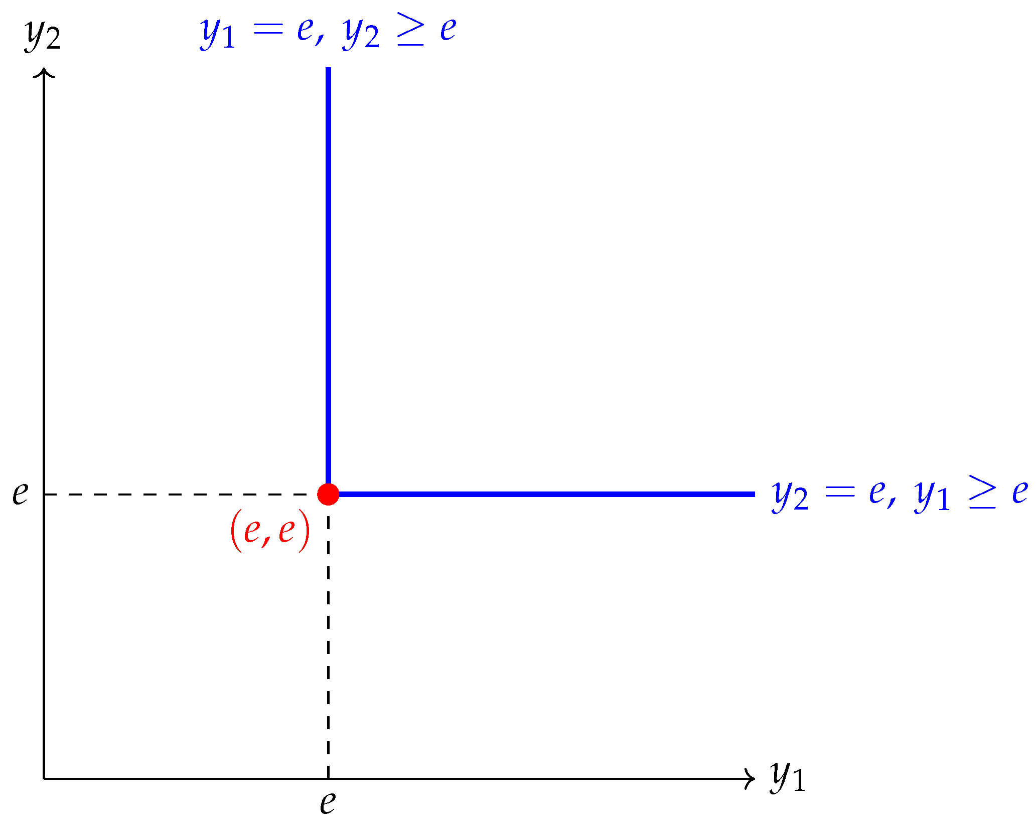
where ${\mathcal{F}}_{\mathfrak{s}}:{\mathbb{X}}^{\left(n\right)}\to \mathbb{R}$ ($i=1,2)$, $\mathcal{C}:{\mathbb{X}}^{\left(n\right)}\to \mathbb{R}$, $\mathcal{D}:{\mathbb{X}}^{\left(n\right)}\to \mathbb{R}$. The feasible set of (P1) is given by (see, Figure 1):

$$F_1:=\{y\in {\mathbb{X}}^{\left(n\right)}:y_1\ge e,y_2=e,\mathit{or},y_2\ge e,y_1=e\}.$$

Let $\tilde{\mathit{\kappa }}=(e,e)\in F_1$. Then, we have

$$\begin{array}{cc}\hfill {\partial }^c{\mathcal{F}}_1\left(p\right)& =co\left\{\left(\begin{array}{c}-p_1^2\\ 0\end{array}\right),\left(\begin{array}{c}{p}_1^2\\ 0\end{array}\right)\right\},\hfill \\ \hfill {\partial }^c{\mathcal{F}}_2\left(p\right)& =\left\{\mathcal{G}{\left(p\right)}^{-1}\left(\begin{array}{c}0\\ {\displaystyle \frac{1}{p_2}}\end{array}\right)\right\}=\left\{\left(\begin{array}{c}0\\ p_2\end{array}\right)\right\},\hfill \\ \hfill {\partial }^c\mathcal{C}\left(p\right)& =\left\{\mathcal{G}{\left(p\right)}^{-1}\left(\begin{array}{c}{\displaystyle \frac{1}{p_1}}\\ 0\end{array}\right)\right\}=\left\{\left(\begin{array}{c}{p}_1\\ 0\end{array}\right)\right\},\hfill \\ \hfill {\partial }^c\mathcal{D}\left(p\right)& =\left\{\mathcal{G}{\left(p\right)}^{-1}\left(\begin{array}{c}0\\ 1\end{array}\right)\right\}=\left\{\left(\begin{array}{c}0\\ p_2^2\end{array}\right)\right\}.\hfill \end{array}$$

From the above expressions, it follows that

$$\begin{array}{cc}\hfill {\mathcal{C}}_{NMMPEC}^{Lin}(\mathcal{L},\tilde{\mathit{\kappa }})& =\{w=(w_1,w_2)\in {\mathbb{R}}^2,w_1=0,w_2=0\},\hfill \\ \hfill {\mathcal{C}}^{Tan}({\mathcal{L}}^1,\tilde{\mathit{\kappa }})& =\{v=(v_1,v_2)\in {\mathbb{R}}^2,v_1\ge 0,v_2=0\},\hfill \\ \hfill {\mathcal{C}}^{Tan}({\mathcal{L}}^2,\tilde{\mathit{\kappa }})& =\{v=(v_1,v_2)\in {\mathbb{R}}^2,v_1=0,v_2\ge 0\}.\hfill \end{array}$$

Consequently, we yield that

$$\bigcap _{\mathfrak{s}=1}^{2}clco{\mathcal{C}}^{Tan}\left({\mathcal{L}}^i,\tilde{\mathit{\kappa }}\right)=\left\{(0,0)\right\}.$$

(18)

Thus, NMMPEC-GGCQ holds at $\tilde{\mathit{\kappa }}=(e,e)\in F_1$. We choose ${\mu }_1={\displaystyle \frac{1}{2}}$, ${\mu }_2={\displaystyle \frac{1}{2}}$, ${\sigma }^{\mathcal{C}}={\displaystyle \frac{e}{2}}$, ${\sigma }^{\mathcal{D}}={\displaystyle \frac{1}{2e}}$. Then, we obtain

$${\mu }_1{\mathsf{\zeta }}_1^{\mathcal{F}}+{\mu }_1{\mathsf{\zeta }}_2^{\mathcal{F}}-{\sigma }^{\mathcal{C}}{\mathsf{\zeta }}^{\mathcal{C}}-{\sigma }^{\mathcal{D}}{\mathsf{\zeta }}^{\mathcal{D}}=(0,0),$$

where ${\mathsf{\zeta }}_1^{\mathcal{F}}={(e^2,0)}^T\in {\partial }^c{\mathcal{F}}_1\left(\tilde{\mathit{\kappa }}\right)$, ${\mathsf{\zeta }}_2^{\mathcal{F}}={(0,e)}^T\in {\partial }^c{\mathcal{F}}_2\left(\tilde{\mathit{\kappa }}\right)$, ${\mathsf{\zeta }}^{\mathcal{C}}={(e,0)}^T\in {\partial }^c\mathcal{C}\left(\tilde{\mathit{\kappa }}\right)$, ${\mathsf{\zeta }}^{\mathcal{D}}={(0,e^2)}^T\in {\partial }^c\mathcal{D}\left(\tilde{\mathit{\kappa }}\right)$. Therefore, every condition in Theorem 2 is verified.

Example 2.

Let ${\mathcal{H}}_2\subset {\mathbb{R}}^2$ denote the Poincaré half-plane, given below:

$${\mathcal{H}}_2:=\{y=(y_1,y_2)\in {\mathbb{R}}^2,y_2>0\}.$$

Then ${\mathcal{H}}_2$ becomes a Riemannian manifold when endowed with the metric defined below (see, [36]):

$${\langle s_1,s_2\rangle }_q=\langle \mathcal{G}\left(q\right)s_1,s_2\rangle ,\forall s_1,s_2\in T_q{\mathcal{H}}_2={\mathbb{R}}^2.$$

and

$$\mathcal{G}\left(q\right)=\left(\begin{array}{cc}{\displaystyle \frac{1}{q_2^2}}& 0\\ 0& {\displaystyle \frac{1}{q_2^2}}\end{array}\right).$$

${\mathcal{H}}_2$ is also a Hadamard manifold (see, [27]). For any $x\in {\mathcal{H}}_2$ and $v\in T_x{\mathcal{H}}_2$, ${exp}_x:T_x{\mathcal{H}}_2\to {\mathcal{H}}_2$ is determined by (see, [27]):

If $v_1=0$,

$${exp}_x\left(v\right)=\left(x_1,x_2{e}^{{\displaystyle \frac{v_2}{x_2}}}\right).$$

If $v_1\ne 0$, ${exp}_x\left(v\right)$ is given by

$$\begin{array}{c}\hfill \left(x_1+{\displaystyle \frac{v_2}{v_1}}+\sqrt{1+{\left({\displaystyle \frac{v_2}{v_1}}\right)}^2}tanh\left(p_{v_1,v_2}\left(1\right)\right),x_2\sqrt{1+{\left({\displaystyle \frac{v_2}{v_1}}\right)}^2}{\displaystyle \frac{1}{cosh\left(q_{\left.v_1,v_2\left(1\right)\right)}\right)}}\right),\end{array}$$

where

$$\begin{array}{c}{p}_{v_1,v_2}\left(t\right)=\left\{\begin{array}{cc}t\sqrt{v_1^2+v_2^2}-arcsinh{\displaystyle \frac{v_2}{v_1}},\hfill & \mathit{if}{v}_1>0,\hfill \\ -t\sqrt{v_1^2+v_2^2}-arcsinh{\displaystyle \frac{v_2}{v_1}},\hfill & \mathit{if}{v}_1<0,\hfill \end{array}\right.\\ q_{v_1,v_2}\left(t\right)=\left\{\begin{array}{cc}t{\displaystyle \frac{\sqrt{v_1^2+v_2^2}}{x_2}}-arcsinh{\displaystyle \frac{v_2}{v_1}},\hfill & \mathit{if}{v}_1>0,\hfill \\ -t{\displaystyle \frac{\sqrt{v_1^2+v_2^2}}{x_2}}-arcsinh{\displaystyle \frac{v_2}{v_1}},\hfill & \mathit{if}{v}_1<0.\hfill \end{array}\right.\end{array}$$

Further ${exp}_x^{-1}:{\mathcal{H}}_2\to T_x{\mathcal{H}}_2$ is given by

$${exp}_x^{-1}\left(y\right)=\left\{\begin{array}{cc}\left(0,x_{2}ln{\displaystyle \frac{y_2}{x_2}}\right),\hfill & \mathit{if}{x}_1=y_1,\hfill \\ {\displaystyle \frac{x_2}{r}}\left(arctanh{\displaystyle \frac{b-x_1}{r}}-arctanh{\displaystyle \frac{b-y_1}{r}}\right)\left(x_2,b-x_1\right),\hfill & \mathit{if}{x}_1\ne y_1.\hfill \end{array}\right.$$

Consider the following NMMPEC on ${\mathcal{H}}_2$:

$$\begin{array}{cc}\hfill \left(P2\right)\mathit{Minimize}\mathcal{F}\left(y\right)& :=\left(\right|y_1|,y_2+|y_2-\frac{3}{4}\left|\right),\hfill \\ \hfill \mathit{subject}\mathit{to}\mathcal{C}\left(y\right)& :=y_2-\frac{1}{2}\ge 0,\hfill \\ \hfill \mathcal{D}\left(y\right)& :=1-y_2\ge 0,\hfill \\ \hfill \mathcal{D}{\left(y\right)}^T\mathcal{C}\left(y\right)& :=(1-y_2)(y_2-\frac{1}{2})=0,\hfill \end{array}$$

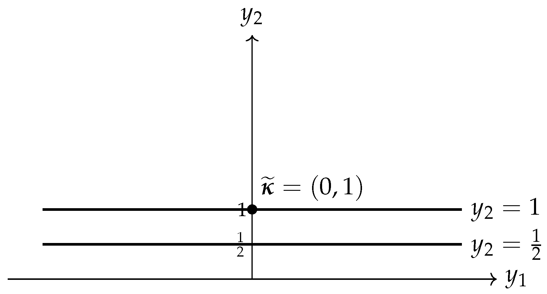
where ${\mathcal{F}}_i:{\mathcal{H}}_2\to \mathbb{R}$ ($\mathfrak{s}=1,2$), $\mathcal{C}:{\mathcal{H}}_2\to \mathbb{R}$, and $\mathcal{D}:{\mathcal{H}}_2\to \mathbb{R}$. $F_2$ refers the feasible set of ($P2$), see, Figure 2. That is

$$F_2:=\{y\in {\mathcal{H}}_2:y_2=\frac{1}{2},y_1\in \mathbb{R}\}\cup \{y\in {\mathcal{H}}_2:y_2=1,y_1\in \mathbb{R}\}.$$

Now, we choose the feasible element $\tilde{\mathit{\kappa }}=(0,1)\in F_2$. The following relations for the tangent and linearizing cones can be easily obtained:

$$\begin{array}{cc}\hfill {\mathcal{C}}_{NMMPEC}^{Lin}(\mathcal{L},\tilde{\mathit{\kappa }})& =\{w=(w_1,w_2)\in {\mathbb{R}}^2:w_2=0\},\hfill \\ \hfill {\mathcal{C}}^{Tan}({\mathcal{L}}^1,\tilde{\mathit{\kappa }})& =\{v=(v_1,v_2)\in {\mathbb{R}}^2:v_2\ge 0,v_1\in \mathbb{R}\},\hfill \\ \hfill {\mathcal{C}}^{Tan}({\mathcal{L}}^2,\tilde{\mathit{\kappa }})& =\{v=(v_1,v_2)\in {\mathbb{R}}^2:v_2\le 0,v_1\in \mathbb{R}\}.\hfill \end{array}$$

Consequently, we yield that

$$\bigcap _{\mathfrak{s}=1}^{2}clco{\mathcal{C}}^{Tan}\left({\mathcal{L}}^i,\tilde{\mathit{\kappa }}\right)=\left\{(0,0)\right\}.$$

(19)

Hence, we conclude that NMMPEC-GGCQ holds at $\tilde{\mathit{\kappa }}=(0,1)\in F_2$.

By choosing multipliers ${\mu }_1={\displaystyle \frac{1}{2}}$, ${\mu }_2={\displaystyle \frac{1}{2}}$, ${\sigma }^{\mathcal{C}}={\displaystyle \frac{3}{2}}$, ${\sigma }^{\mathcal{D}}=0$, we obtain

$${\mu }_1{\mathsf{\zeta }}_1^{\mathcal{F}}+{\mu }_2{\mathsf{\zeta }}_2^{\mathcal{F}}-{\sigma }^{\mathcal{C}}{\mathsf{\zeta }}^{\mathcal{C}}-{\sigma }^{\mathcal{D}}{\mathsf{\zeta }}^{\mathcal{D}}=(0,0),$$

for suitable selections ${\mathsf{\zeta }}_1^{\mathcal{F}}\in {\partial }^c{\mathcal{F}}_1\left(\tilde{\mathit{\kappa }}\right)$, ${\mathsf{\zeta }}_2^{\mathcal{F}}\in {\partial }^c{\mathcal{F}}_2\left(\tilde{\mathit{\kappa }}\right)$, ${\mathsf{\zeta }}^{\mathcal{C}}\in {\partial }^c\mathcal{C}\left(\tilde{\mathit{\kappa }}\right)$, ${\mathsf{\zeta }}^{\mathcal{D}}\in {\partial }^c\mathcal{D}\left(\tilde{\mathit{\kappa }}\right)$. Hence, every requirement of Theorem 2 is satisfied.

In this section, an NMMPEC has been considered on Hadamard manifolds. Further, we have deduced KKT-type necessary conditions for Pareto efficiency for NMMPEC by employing the GGCQ.

4. Constraint Qualifications for NMMPEC on Hadamard Manifolds

We now adapt various classical constraint qualifications and investigate their NMMPEC-specific counterparts on manifolds.

Definition 11.

The NMMPEC-adapt Abadie constraint qualification (NMMPEC-ACQ) holds at $\tilde{\mathit{\kappa }}\in \mathcal{S}$ if:

$${\mathcal{C}}_{NMMPEC}^{Lin}\left(\mathcal{L},\tilde{\mathit{\kappa }}\right)\subseteq {\mathcal{C}}^{Tan}\left(\mathcal{L},\tilde{\mathit{\kappa }}\right).$$

(20)

Definition 12.

The NMMPEC-adapt generalized Abadie CQ (NMMPEC-GACQ) holds at $\tilde{\mathit{\kappa }}\in \mathcal{S}$ if:

$${\mathcal{C}}_{NMMPEC}^{Lin}\left(\mathcal{L},\tilde{\mathit{\kappa }}\right)\subseteq \bigcap _{i\in \mathcal{I}}{\mathcal{C}}^{Tan}\left({\mathcal{L}}^i,\tilde{\mathit{\kappa }}\right).$$

(21)

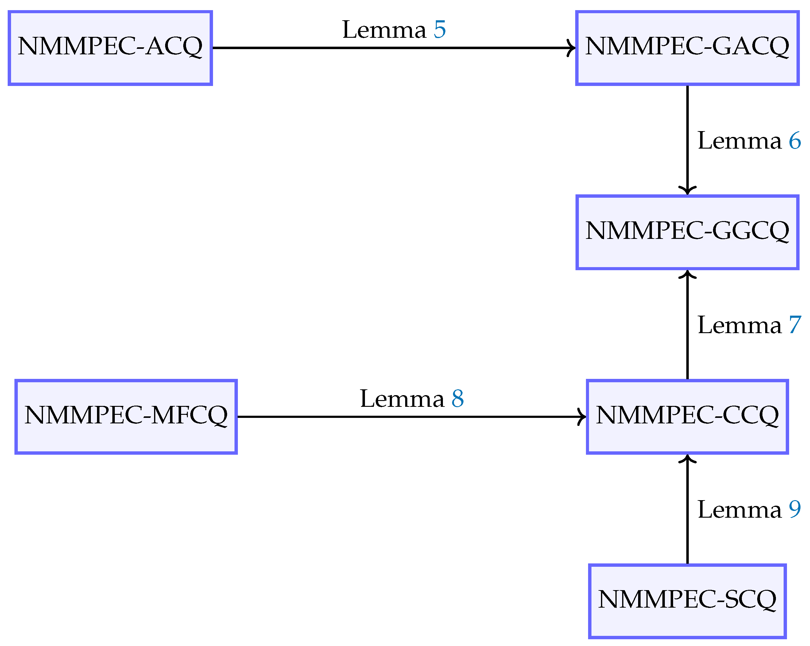
The lemmas stated below are straightforward consequences of the definitions of NMMPEC-ACQ and NMMPEC-GACQ.

Lemma 5.

If NMMPEC-ACQ is satisfied at $\tilde{\mathit{\kappa }}\in \mathcal{S}$, then NMMPEC-GACQ is also satisfied at $\tilde{\mathit{\kappa }}$.

Lemma 6.

If NMMPEC-GACQ holds at $\tilde{\mathit{\kappa }}\in \mathcal{S}$, then NMMPEC-GGCQ holds at $\tilde{\mathit{\kappa }}$.

The following definitions are extended from Maeda [22] for NMMPEC on Hadamard manifolds.

Definition 13.

The NMMPEC-adapt Cottle-type CQ (NMMPEC-CCQ) holds at $\tilde{\mathit{\kappa }}\in \mathcal{S}$, if for every $r\in \mathcal{I}$ the subsequent system:

$$\begin{array}{cc}\hfill {\mathcal{F}}_{\mathfrak{p}}^{\circ }(\tilde{\mathit{\kappa }},\widehat{o})<0,& \forall \mathfrak{p}\in \mathcal{I}\mathrm{and}\mathfrak{p}\ne r,\hfill \\ \hfill {\mathcal{W}}_{\mathfrak{p}}^{\circ }(\tilde{\mathit{\kappa }},\widehat{o})<0,& \forall \mathfrak{p}\in {\mathcal{A}}^{\mathcal{W}}\left(\tilde{\mathit{\kappa }}\right),\hfill \\ \hfill {\mathcal{V}}_{\mathfrak{p}}^{\circ }(\tilde{\mathit{\kappa }},\widehat{o})=0,& \forall \mathfrak{p}\in {\mathcal{I}}^{\mathcal{V}},\hfill \\ \hfill {\mathcal{C}}_{\mathfrak{p}}^{\circ }(\tilde{\mathit{\kappa }},\widehat{o})=0,& \forall \mathfrak{p}\in {\mathcal{E}}_{0+},\hfill \\ \hfill {\mathcal{D}}_{\mathfrak{p}}^{\circ }(\tilde{\mathit{\kappa }},\widehat{o})=0,& \forall \mathfrak{p}\in {\mathcal{E}}_{+0},\hfill \\ \hfill {-\mathcal{C}}_{\mathfrak{p}}^{\circ }(\tilde{\mathit{\kappa }},\widehat{o})<0,& \forall \mathfrak{p}\in {\mathcal{E}}_{00},\hfill \\ \hfill {-\mathcal{D}}_{\mathfrak{p}}^{\circ }(\tilde{\mathit{\kappa }},\widehat{o})<0,& \forall \mathfrak{p}\in {\mathcal{E}}_{00},\hfill \end{array}$$

(22)

has a solution $\widehat{o}\in T_{\tilde{\mathit{\kappa }}}{\mathbb{X}}^{\left(n\right)}$.

Definition 14.

The NMMPEC-adapt Slater-type CQ (NMMPEC-SCQ) holds at $\tilde{\mathit{\kappa }}\in \mathcal{S}$ if ${\mathcal{F}}_{\mathfrak{p}}$$(\mathfrak{p}\in \mathcal{I}$), and ${\mathcal{W}}_{\mathfrak{p}}$$(\mathfrak{p}\in {\mathcal{I}}^{\mathcal{W}})$, are geodesic convex, ${\mathcal{C}}_{\mathfrak{p}}$$(\mathfrak{p}\in {\mathcal{E}}_{00})$, ${\mathcal{D}}_{\mathfrak{p}}$$(\mathfrak{p}\in {\mathcal{E}}_{00})$ are geodesic concave, ${\mathcal{C}}_{\mathfrak{p}}$$(\mathfrak{p}\in {\mathcal{E}}_{0+})$, ${\mathcal{D}}_{\mathfrak{p}}$$(\mathfrak{p}\in {\mathcal{E}}_{+0})$, ${\mathcal{V}}_{\mathfrak{p}}$$(\mathfrak{p}\in {\mathcal{I}}^{\mathcal{V}})$ are geodesic affine. Furthermore, for every $k\in \mathcal{I}$ the subsequent system:

$$\begin{array}{cccc}\hfill {\mathcal{F}}_{\mathfrak{p}}\left(z\right)& <{\mathcal{F}}_{\mathfrak{p}}\left(\tilde{\mathit{\kappa }}\right),\hfill & \hfill & \forall \mathfrak{p}\in \mathcal{I}and\mathfrak{p}\ne k,\hfill \\ \hfill {\mathcal{W}}_{\mathfrak{p}}\left(z\right)& <0,\hfill & \hfill & \forall \mathfrak{p}\in {\mathcal{A}}^{\mathcal{W}}\left(\tilde{\mathit{\kappa }}\right),\hfill \\ \hfill {\mathcal{V}}_{\mathfrak{p}}\left(z\right)& =0,\hfill & \hfill & \forall \mathfrak{p}\in {\mathcal{I}}^{\mathcal{V}},\hfill \\ \hfill {\mathcal{C}}_{\mathfrak{p}}\left(z\right)& =0,\hfill & \hfill & \forall \mathfrak{p}\in {\mathcal{E}}_{0+},\hfill \\ \hfill {\mathcal{D}}_{\mathfrak{p}}\left(z\right)& =0,\hfill & \hfill & \forall \mathfrak{p}\in {\mathcal{E}}_{+0},\hfill \\ \hfill {\mathcal{C}}_{\mathfrak{p}}\left(z\right)& >0,\hfill & \hfill & \forall \mathfrak{p}\in {\mathcal{E}}_{00},\hfill \\ \hfill {\mathcal{D}}_{\mathfrak{p}}\left(z\right)& >0,\hfill & \hfill & \forall \mathfrak{p}\in {\mathcal{E}}_{00}.\hfill \end{array}$$

(23)

has a solution $z\in {\mathbb{X}}^{\left(n\right)}$.

Definition 15.

The NMMPEC-adapt Mangasarian-Fromovitz CQ (NMMPEC-MFCQ) holds at $\tilde{\mathit{\kappa }}\in \mathcal{S}$ if ${\mathsf{\zeta }}_{\mathfrak{p}}^{\mathcal{F}}$$({\mathsf{\zeta }}_{\mathfrak{p}}^{\mathcal{F}}\in {\partial }^c{\mathcal{F}}_{\mathfrak{p}}\left(\tilde{\mathit{\kappa }}\right),\mathfrak{p}\in \mathcal{I})$, ${\mathsf{\zeta }}_{\mathfrak{p}}^{\mathcal{V}}$$({\mathsf{\zeta }}_{\mathfrak{p}}^{\mathcal{V}}\in {\partial }^c{\mathcal{V}}_{\mathfrak{p}}\left(\tilde{\mathit{\kappa }}\right),\mathfrak{p}\in {\mathcal{I}}^{\mathcal{V}})$, ${\mathsf{\zeta }}_{\mathfrak{p}}^{\mathcal{C}}$$({\mathsf{\zeta }}_{\mathfrak{p}}^{\mathcal{C}}\in {\partial }^c{\mathcal{C}}_{\mathfrak{p}}\left(\tilde{\mathit{\kappa }}\right),\mathfrak{p}\in {\mathcal{E}}_{0+}\cup {\mathcal{E}}_{00})$, ${\mathsf{\zeta }}_{\mathfrak{p}}^{\mathcal{D}}$$({\mathsf{\zeta }}_{\mathfrak{p}}^{\mathcal{D}}\in {\partial }^c{\mathcal{D}}_{\mathfrak{p}}\left(\tilde{\mathit{\kappa }}\right),\mathfrak{p}\in {\mathcal{E}}_{+0}\cup {\mathcal{E}}_{00})$ are linearly independent, and moreover

$$\begin{array}{cc}\hfill {\mathcal{F}}_{\mathfrak{p}}^{\circ }(\tilde{\mathit{\kappa }},v)=0,& \forall \mathfrak{p}\in \mathcal{I},\hfill \\ \hfill {\mathcal{W}}_{\mathfrak{p}}^{\circ }(\tilde{\mathit{\kappa }},v)<0,& \forall \mathfrak{p}\in {\mathcal{A}}^{\mathcal{W}}\left(\tilde{\mathit{\kappa }}\right),\hfill \\ \hfill {\mathcal{V}}_{\mathfrak{p}}^{\circ }(\tilde{\mathit{\kappa }},v)=0,& \forall \mathfrak{p}\in {\mathcal{I}}^{\mathcal{V}},\hfill \\ \hfill {\mathcal{C}}_{\mathfrak{p}}^{\circ }(\tilde{\mathit{\kappa }},v)=0,& \forall \mathfrak{p}\in {\mathcal{E}}_{0+},\hfill \\ \hfill {\mathcal{D}}_{\mathfrak{p}}^{\circ }(\tilde{\mathit{\kappa }},v)=0,& \forall \mathfrak{p}\in {\mathcal{E}}_{+0},\hfill \\ \hfill {-\mathcal{C}}_{\mathfrak{p}}^{\circ }(\tilde{\mathit{\kappa }},v)<0,& \forall \mathfrak{p}\in {\mathcal{E}}_{00},\hfill \\ \hfill {-\mathcal{D}}_{\mathfrak{p}}^{\circ }(\tilde{\mathit{\kappa }},v)<0,& \forall \mathfrak{p}\in {\mathcal{E}}_{00},\hfill \end{array}$$

(24)

has a solution $v\in T_{\tilde{\mathit{\kappa }}}{\mathbb{X}}^{\left(n\right)}$.

The lemmas presented below establish several nontrivial relationships among the constraint qualifications specifically developed for $\left(\mathrm{NMMPEC}\right)$.

Lemma 7.

If NMMPEC-CCQ holds at $\tilde{\mathit{\kappa }}\in \mathcal{S}$, then NMMPEC-GGCQ also holds at $\tilde{\mathit{\kappa }}$.

Proof. 

It is given that $\tilde{\mathit{\kappa }}\in \mathcal{S}$. Moreover, CCQ is satisfied at $\tilde{\mathit{\kappa }}\in \mathcal{S}$. Hence, some $\widehat{o}\in T_{\tilde{\mathit{\kappa }}}{\mathbb{X}}^{\left(n\right)}$ exists, such that (22) hold true. On the other hand, there exists some $\widehat{o}\in T_{\tilde{\mathit{\kappa }}}{\mathbb{X}}^{\left(n\right)}$ such that

$$\begin{array}{cccccc}\hfill & \langle {\mathsf{\zeta }}_{\mathfrak{p}}^{\mathcal{F}},\widehat{o}\rangle <0,\hfill & \hfill & \forall {\mathsf{\zeta }}_{\mathfrak{p}}^{\mathcal{F}}\in {\partial }^c{\mathcal{F}}_{\mathfrak{p}}\left(\tilde{\mathit{\kappa }}\right),\hfill & \hfill & \forall \mathfrak{p}\in \mathcal{I}\setminus \left\{1\right\},\hfill \\ \hfill & \langle {\mathsf{\zeta }}_{\mathfrak{p}}^{\mathcal{W}},\widehat{o}\rangle <0,\hfill & \hfill & \forall {\mathsf{\zeta }}_{\mathfrak{p}}^{\mathcal{W}}\in {\partial }^c{\mathcal{W}}_{\mathfrak{p}}\left(\tilde{\mathit{\kappa }}\right),\hfill & \hfill & \forall \mathfrak{p}\in {\mathcal{A}}^{\mathcal{W}},\hfill \\ \hfill & \langle {\mathsf{\zeta }}_{\mathfrak{p}}^{\mathcal{V}},\widehat{o}\rangle =0,\hfill & \hfill & \forall {\mathsf{\zeta }}_{\mathfrak{p}}^{\mathcal{V}}\in {\partial }^c{\mathcal{V}}_{\mathfrak{p}}\left(\tilde{\mathit{\kappa }}\right),\hfill & \hfill & \forall \mathfrak{p}\in {\mathcal{I}}^{\mathcal{V}},\hfill \\ \hfill & \langle {\mathsf{\zeta }}_{\mathfrak{p}}^{\mathcal{C}},\widehat{o}\rangle =0,\hfill & \hfill & \forall {\mathsf{\zeta }}_{\mathfrak{p}}^{\mathcal{C}}\in {\partial }^c{\mathcal{C}}_{\mathfrak{p}}\left(\tilde{\mathit{\kappa }}\right),\hfill & \hfill & \forall \mathfrak{p}\in {\mathcal{E}}_{0+},\hfill \\ \hfill & \langle {\mathsf{\zeta }}_{\mathfrak{p}}^{\mathcal{D}},\widehat{o}\rangle =0,\hfill & \hfill & \forall {\mathsf{\zeta }}_{\mathfrak{p}}^{\mathcal{D}}\in {\partial }^c{\mathcal{D}}_{\mathfrak{p}}\left(\tilde{\mathit{\kappa }}\right),\hfill & \hfill & \forall \mathfrak{p}\in {\mathcal{E}}_{+0},\hfill \\ \hfill & \langle {\mathsf{\zeta }}_{\mathfrak{p}}^{\mathcal{C}},\widehat{o}\rangle >0,\hfill & \hfill & \forall {\mathsf{\zeta }}_{\mathfrak{p}}^{\mathcal{C}}\in {\partial }^c{\mathcal{C}}_{\mathfrak{p}}\left(\tilde{\mathit{\kappa }}\right),\hfill & \hfill & \forall \mathfrak{p}\in {\mathcal{E}}_{00},\hfill \\ \hfill & \langle {\mathsf{\zeta }}_{\mathfrak{p}}^{\mathcal{D}},\widehat{o}\rangle >0,\hfill & \hfill & \forall {\mathsf{\zeta }}_{\mathfrak{p}}^{\mathcal{D}}\in {\partial }^c{\mathcal{D}}_{\mathfrak{p}}\left(\tilde{\mathit{\kappa }}\right),\hfill & \hfill & \forall \mathfrak{p}\in {\mathcal{E}}_{00}.\hfill \end{array}$$

(25)

Let $v\in {\mathcal{C}}_{NMMPEC}^{Lin}\left(\mathcal{L},\tilde{\mathit{\kappa }}\right)$. Then, in view of Definition 9, it follows that

$$\begin{array}{cccccc}\hfill & \langle {\mathsf{\zeta }}_{\mathfrak{p}}^{\mathcal{F}},v\rangle \le 0,\hfill & \hfill & \forall {\mathsf{\zeta }}_{\mathfrak{p}}^{\mathcal{F}}\in {\partial }^c{\mathcal{F}}_{\mathfrak{p}}\left(\tilde{\mathit{\kappa }}\right),\hfill & \hfill & \forall \mathfrak{p}\in \mathcal{I},\hfill \\ \hfill & \langle {\mathsf{\zeta }}_{\mathfrak{p}}^{\mathcal{W}},v\rangle \le 0,\hfill & \hfill & \forall {\mathsf{\zeta }}_{\mathfrak{p}}^{\mathcal{W}}\in {\partial }^c{\mathcal{W}}_{\mathfrak{p}}\left(\tilde{\mathit{\kappa }}\right),\hfill & \hfill & \forall \mathfrak{p}\in {\mathcal{A}}^{\mathcal{W}},\hfill \\ \hfill & \langle {\mathsf{\zeta }}_{\mathfrak{p}}^{\mathcal{V}},v\rangle =0,\hfill & \hfill & \forall {\mathsf{\zeta }}_{\mathfrak{p}}^{\mathcal{V}}\in {\partial }^c{\mathcal{V}}_{\mathfrak{p}}\left(\tilde{\mathit{\kappa }}\right),\hfill & \hfill & \forall \mathfrak{p}\in {\mathcal{I}}^{\mathcal{V}},\hfill \\ \hfill & \langle {\mathsf{\zeta }}_{\mathfrak{p}}^{\mathcal{C}},v\rangle =0,\hfill & \hfill & \forall {\mathsf{\zeta }}_{\mathfrak{p}}^{\mathcal{C}}\in {\partial }^c{\mathcal{C}}_{\mathfrak{p}}\left(\tilde{\mathit{\kappa }}\right),\hfill & \hfill & \forall \mathfrak{p}\in {\mathcal{E}}_{0+},\hfill \\ \hfill & \langle {\mathsf{\zeta }}_{\mathfrak{p}}^{\mathcal{D}},v\rangle =0,\hfill & \hfill & \forall {\mathsf{\zeta }}_{\mathfrak{p}}^{\mathcal{D}}\in {\partial }^c{\mathcal{D}}_{\mathfrak{p}}\left(\tilde{\mathit{\kappa }}\right),\hfill & \hfill & \forall \mathfrak{p}\in {\mathcal{E}}_{+0},\hfill \\ \hfill & \langle {\mathsf{\zeta }}_{\mathfrak{p}}^{\mathcal{C}},v\rangle \ge 0,\hfill & \hfill & \forall {\mathsf{\zeta }}_{\mathfrak{p}}^{\mathcal{C}}\in {\partial }^c{\mathcal{C}}_{\mathfrak{p}}\left(\tilde{\mathit{\kappa }}\right),\hfill & \hfill & \forall \mathfrak{p}\in {\mathcal{E}}_{00},\hfill \\ \hfill & \langle {\mathsf{\zeta }}_{\mathfrak{p}}^{\mathcal{D}},v\rangle \ge 0,\hfill & \hfill & \forall {\mathsf{\zeta }}_{\mathfrak{p}}^{\mathcal{D}}\in {\partial }^c{\mathcal{D}}_{\mathfrak{p}}\left(\tilde{\mathit{\kappa }}\right),\hfill & \hfill & \forall \mathfrak{p}\in {\mathcal{E}}_{00}.\hfill \end{array}$$

(26)

We assert that $v\in {\mathcal{C}}^{Tan}\left({\mathcal{L}}^1,\tilde{\mathit{\kappa }}\right)$. Consider a sequence ${\left\{b_n\right\}}_{n=1}^{\infty }\downarrow 0$. Define ${\left\{v_n\right\}}_{n=1}^{\infty }$ as

$$v_n:=v+b_n\widehat{o},\forall n\in \mathbb{N}.$$

(27)

Evidently, $v_n\to v$ as $n\to \infty$. In light of (25), (26) and (27), we have

$$\begin{array}{cccc}\hfill & 〈{\mathsf{\zeta }}_{\mathfrak{p}}^{\mathcal{F}},v_n〉<0,\hfill & \hfill & \forall {\mathsf{\zeta }}_{\mathfrak{p}}^{\mathcal{F}}\in {\partial }^c{\mathcal{F}}_{\mathfrak{p}}\left(\tilde{\mathit{\kappa }}\right),\forall \mathfrak{p}\in \mathcal{I}\setminus \left\{1\right\},\hfill \\ \hfill & 〈{\mathsf{\zeta }}_{\mathfrak{p}}^{\mathcal{W}},v_n〉<0,\hfill & \hfill & \forall {\mathsf{\zeta }}_{\mathfrak{p}}^{\mathcal{W}}\in {\partial }^c{\mathcal{W}}_{\mathfrak{p}}\left(\tilde{\mathit{\kappa }}\right),\forall \mathfrak{p}\in \mathcal{A}\left(\tilde{\mathit{\kappa }}\right),\hfill \\ \hfill & 〈{\mathsf{\zeta }}_{\mathfrak{p}}^{\mathcal{V}},v_n〉=0,\hfill & \hfill & \forall {\mathsf{\zeta }}_{\mathfrak{p}}^{\mathcal{V}}\in {\partial }^c{\mathcal{V}}_{\mathfrak{p}}\left(\tilde{\mathit{\kappa }}\right),\forall \mathfrak{p}\in {\mathcal{I}}^{\mathcal{V}},\hfill \\ \hfill & 〈{\mathsf{\zeta }}_{\mathfrak{p}}^{\mathcal{C}},v_n〉=0,\hfill & \hfill & \forall {\mathsf{\zeta }}_{\mathfrak{p}}^{\mathcal{C}}\in {\partial }^c{\mathcal{C}}_{\mathfrak{p}}\left(\tilde{\mathit{\kappa }}\right),\forall \mathfrak{p}\in {\mathcal{E}}_{0+},\hfill \\ \hfill & 〈{\mathsf{\zeta }}_{\mathfrak{p}}^{\mathcal{D}},v_n〉=0,\hfill & \hfill & \forall {\mathsf{\zeta }}_{\mathfrak{p}}^{\mathcal{D}}\in {\partial }^c{\mathcal{D}}_{\mathfrak{p}}\left(\tilde{\mathit{\kappa }}\right),\forall \mathfrak{p}\in {\mathcal{E}}_{+0},\hfill \\ \hfill & 〈{\mathsf{\zeta }}_{\mathfrak{p}}^{\mathcal{C}},v_n〉\ge 0,\hfill & \hfill & \forall {\mathsf{\zeta }}_{\mathfrak{p}}^{\mathcal{C}}\in {\partial }^c{\mathcal{C}}_{\mathfrak{p}}\left(\tilde{\mathit{\kappa }}\right),\forall \mathfrak{p}\in {\mathcal{E}}_{00},\hfill \\ \hfill & 〈{\mathsf{\zeta }}_{\mathfrak{p}}^{\mathcal{D}},v_n〉\ge 0,\hfill & \hfill & \forall {\mathsf{\zeta }}_{\mathfrak{p}}^{\mathcal{D}}\in {\partial }^c{\mathcal{D}}_{\mathfrak{p}}\left(\tilde{\mathit{\kappa }}\right),\forall \mathfrak{p}\in {\mathcal{E}}_{00}.\hfill \end{array}$$

For each element in ${\left\{v_n\right\}}_{n=1}^{\infty }$, let us consider another sequence ${\left\{{\lambda }_{n_k}\right\}}_{k=1}^{\infty }\downarrow 0$. Hence, we may define ${\left\{z_{n_k}\right\}}_{k=1}^{\infty }$ as

$$z_{n_k}:={exp}_{\tilde{\mathit{\kappa }}}\left({\lambda }_{n_k}{v}_n\right),\forall k\in \mathbb{N}.$$

Evidently, $\left\{z_{n_k}\right\}\to \tilde{\mathit{\kappa }}$ as $k\to \infty$. In view of Theorem 1, for every $n_k\in \mathbb{N}$, some ${\delta }_{n_k}\in (0,1)$, $a_{n_k}=\gamma \left({\delta }_{n_k}\right)$, and ${\vartheta }_{n_k}\in {\partial }^c{\mathcal{F}}_{\mathfrak{p}}\left(a_{n_k}\right)$ exist, satisfying

$${\mathcal{F}}_{\mathfrak{p}}\left(z_{n_k}\right)-{\mathcal{F}}_{\mathfrak{p}}\left(\tilde{\mathit{\kappa }}\right)=〈{\vartheta }_{n_k},{\gamma }^{\prime }\left({\delta }_{n_k}\right)〉,\forall \mathfrak{p}\in \mathcal{I}\setminus \left\{1\right\},$$

(28)

where

$$\gamma \left({\delta }_{n_k}\right):={exp}_{\tilde{\mathit{\kappa }}}\left({\delta }_{n_k}{exp}_{\tilde{\mathit{\kappa }}}^{-1}\left(z_{n_k}\right)\right).$$

It is obvious that as ${\delta }_{n_k}\to 0$, $a_{n_k}\to \tilde{\mathit{\kappa }}$. From Lemma 1, there exists some subsequence ${\left\{{\vartheta }_{n_k}^r\right\}}_{r=1}^{\infty }$ of ${\vartheta }_n$, such that ${\vartheta }_{n_k}^r\to \widehat{\vartheta }$ and $\widehat{\vartheta }\in {\partial }^c{\mathcal{F}}_{\mathfrak{p}}\left(\tilde{\mathit{\kappa }}\right)$$(\mathfrak{p}\in \mathcal{I}\setminus \{1\left\}\right)$. In light of (28), for every $r\in \mathbb{N}$, we get

$${\mathcal{F}}_{\mathfrak{p}}\left(z_{n_k}^r\right)-{\mathcal{F}}_{\mathfrak{p}}\left(\tilde{\mathit{\kappa }}\right)=〈{\vartheta }_{n_k}^r,{\gamma }^{\prime }\left({\delta }_{n_k}^r\right)〉,\forall \mathfrak{p}\in \mathcal{I}\setminus \left\{1\right\}.$$

Since $〈{\vartheta }_{n_k}^r,{\gamma }^{\prime }\left({\delta }_{n_k}^r\right)〉\to \langle \widehat{\vartheta },v_n\rangle <0$, for large enough k, we obtain

$$\begin{array}{c}\hfill {\mathcal{F}}_{\mathfrak{p}}\left(z_{n_k}\right)<{\mathcal{F}}_{\mathfrak{p}}\left(\tilde{\mathit{\kappa }}\right),\forall \mathfrak{p}\in \mathcal{I}\setminus \left\{1\right\}.\end{array}$$

(29)

Analogously, for large enough k, for every $\mathfrak{p}\in {\mathcal{A}}^{\mathcal{W}}\left(\tilde{\mathit{\kappa }}\right)$, we obtain

$$\begin{array}{c}\hfill {\mathcal{W}}_{\mathfrak{p}}\left(z_{n_k}\right)=0.\end{array}$$

(30)

For every $j\notin {\mathcal{A}}^{\mathcal{W}}\left(\tilde{\mathit{\kappa }}\right)$, it follows from the continuity property of ${\mathcal{W}}_{\mathfrak{p}}$ that

$${\mathcal{W}}_{\mathfrak{p}}\left(z_{n_k}\right)<0,\mathrm{for}\mathrm{large}\mathrm{enough}k.$$

(31)

Proceeding analogously, we can obtain

$$\begin{array}{cccc}\hfill {\mathcal{V}}_{\mathfrak{p}}\left(z_{n_k}\right)& =0,\forall \mathfrak{p}\in {\mathcal{I}}^{\mathcal{V}},\hfill & \hfill & \mathrm{for}\mathrm{large}\mathrm{enough}k,\hfill \\ \hfill {\mathcal{C}}_{\mathfrak{p}}\left(z_{n_k}\right)& =0,\forall \mathfrak{p}\in {\mathcal{E}}_{0+},\hfill & \hfill & \mathrm{for}\mathrm{large}\mathrm{enough}k,\hfill \\ \hfill {\mathcal{D}}_{\mathfrak{p}}\left(z_{n_k}\right)& =0,\forall \mathfrak{p}\in {\mathcal{E}}_{+0},\hfill & \hfill & \mathrm{for}\mathrm{large}\mathrm{enough}k,\hfill \\ \hfill {\mathcal{C}}_{\mathfrak{p}}\left(z_{n_k}\right)& \ge 0,\forall \mathfrak{p}\in {\mathcal{E}}_{00},\hfill & \hfill & \mathrm{for}\mathrm{large}\mathrm{enough}k,\hfill \\ \hfill {\mathcal{D}}_{\mathfrak{p}}\left(z_{n_k}\right)& \ge 0,\forall \mathfrak{p}\in {\mathcal{E}}_{00},\hfill & \hfill & \mathrm{for}\mathrm{large}\mathrm{enough}k,\hfill \end{array}$$

(32)

Then it follows from (29), (30), (31) and (32) that

$$z_{n_k}=\left({exp}_{\tilde{\mathit{\kappa }}}\left({\lambda }_{n_k}{v}_n\right)\right)\in {\mathcal{L}}^1,\mathrm{for}\mathrm{large}\mathrm{enough}k.$$

Without restricting generality, it is relevant to assume that $z_{n_k}\in {\mathcal{L}}^1$ for all k. This indicates that

$$v\in {\mathcal{C}}^{Tan}\left({\mathcal{L}}^1,\tilde{\mathit{\kappa }}\right).$$

Similarly, for any choice of $k\in \mathcal{I}\setminus \left\{1\right\}$, $v\in {\mathcal{C}}^{Tan}\left({\mathcal{L}}^k,\tilde{\mathit{\kappa }}\right)$ holds. Hence, we obtain

$$v\in \bigcap _{k\in \mathcal{I}}{\mathcal{C}}^{Tan}\left({\mathcal{L}}^k,\tilde{\mathit{\kappa }}\right)\subseteq \bigcap _{k\in \mathcal{I}}clco{\mathcal{C}}^{Tan}\left({\mathcal{L}}^k,\tilde{\mathit{\kappa }}\right).$$

Therefore, the proof is complete. □

Lemma 8.

If NMMPEC-MFCQ holds at $\tilde{\mathit{\kappa }}\in \mathcal{S}$, then NMMPEC-CCQ holds at $\tilde{\mathit{\kappa }}$.

Proof. 

It is given that NMMPEC-MFCQ holds at $\tilde{\mathit{\kappa }}\in \mathcal{S}$. This implies that ${\mathsf{\zeta }}_{\mathfrak{p}}^{\mathcal{F}}$$({\mathsf{\zeta }}_{\mathfrak{p}}^{\mathcal{F}}\in {\partial }^c{\mathcal{F}}_{\mathfrak{p}}\left(\tilde{\mathit{\kappa }}\right),\mathfrak{p}\in \mathcal{I})$, ${\mathsf{\zeta }}_{\mathfrak{p}}^{\mathcal{V}}$$({\mathsf{\zeta }}_{\mathfrak{p}}^{\mathcal{V}}\in {\partial }^c{\mathcal{V}}_{\mathfrak{p}}\left(\tilde{\mathit{\kappa }}\right),\mathfrak{p}\in {\mathcal{I}}^{\mathcal{V}})$, ${\mathsf{\zeta }}_{\mathfrak{p}}^{\mathcal{C}}$$({\mathsf{\zeta }}_{\mathfrak{p}}^{\mathcal{C}}\in {\partial }^c{\mathcal{C}}_{\mathfrak{p}}\left(\tilde{\mathit{\kappa }}\right),\mathfrak{p}\in {\mathcal{E}}_{0+}\cup {\mathcal{E}}_{00})$, ${\mathsf{\zeta }}_{\mathfrak{p}}^{\mathcal{D}}$$({\mathsf{\zeta }}_{\mathfrak{p}}^{\mathcal{D}}\in {\partial }^c{\mathcal{D}}_{\mathfrak{p}}\left(\tilde{\mathit{\kappa }}\right),\mathfrak{p}\in {\mathcal{E}}_{+0}\cup {\mathcal{E}}_{00})$ are linearly independent.

Again, some $\tilde{u}\in T_{\tilde{\mathit{\kappa }}}{\mathbb{X}}^{\left(n\right)}$ exist, satisfying (24). Hence, we have

$$\begin{array}{cccc}\hfill & 〈{\mathsf{\zeta }}_{\mathfrak{p}}^{\mathcal{F}},\tilde{u}〉=0,\forall {\mathsf{\zeta }}_{\mathfrak{p}}^{\mathcal{F}}\in {\partial }^c{\mathcal{F}}_{\mathfrak{p}}\left(\tilde{\mathit{\kappa }}\right),\hfill & \hfill & \forall \mathfrak{p}\in \mathcal{I},\hfill \\ \hfill & 〈{\mathsf{\zeta }}_{\mathfrak{p}}^{\mathcal{W}},\tilde{u}〉<0,\forall {\mathsf{\zeta }}_{\mathfrak{p}}^{\mathcal{W}}\in {\partial }^c{\mathcal{W}}_{\mathfrak{p}}\left(\tilde{\mathit{\kappa }}\right),\hfill & \hfill & \forall \mathfrak{p}\in {\mathcal{A}}^{\mathcal{W}}\left(\tilde{\mathit{\kappa }}\right),\hfill \\ \hfill & 〈{\mathsf{\zeta }}_{\mathfrak{p}}^{\mathcal{V}},\tilde{u}〉=0,\forall {\mathsf{\zeta }}_{\mathfrak{p}}^{\mathcal{V}}\in {\partial }^c{\mathcal{V}}_{\mathfrak{p}}\left(\tilde{\mathit{\kappa }}\right),\hfill & \hfill & \forall \mathfrak{p}\in {\mathcal{I}}^{\mathcal{V}},\hfill \\ \hfill & 〈{\mathsf{\zeta }}_{\mathfrak{p}}^{\mathcal{C}},\tilde{u}〉=0,\forall {\mathsf{\zeta }}_{\mathfrak{p}}^{\mathcal{C}}\in {\partial }_c{\mathcal{C}}_{\mathfrak{p}}\left(\tilde{\mathit{\kappa }}\right),\hfill & \hfill & \forall \mathfrak{p}\in {\mathcal{E}}_{0+},\hfill \\ \hfill & 〈{\mathsf{\zeta }}_{\mathfrak{p}}^{\mathcal{D}},\tilde{u}〉=0,\forall {\mathsf{\zeta }}_{\mathfrak{p}}^{\mathcal{D}}\in {\partial }_c{\mathcal{D}}_{\mathfrak{p}}\left(\tilde{\mathit{\kappa }}\right),\hfill & \hfill & \forall \mathfrak{p}\in {\mathcal{E}}_{+0},\hfill \\ \hfill & 〈{\mathsf{\zeta }}_{\mathfrak{p}}^{\mathcal{C}},\tilde{u}〉>0,\forall {\mathsf{\zeta }}_{\mathfrak{p}}^{\mathcal{C}}\in {\partial }_c{\mathcal{C}}_{\mathfrak{p}}\left(\tilde{\mathit{\kappa }}\right),\hfill & \hfill & \forall \mathfrak{p}\in {\mathcal{E}}_{00},\hfill \\ \hfill & 〈{\mathsf{\zeta }}_{\mathfrak{p}}^{\mathcal{D}},\tilde{u}〉>0,\forall {\mathsf{\zeta }}_{\mathfrak{p}}^{\mathcal{D}}\in {\partial }^c{\mathcal{D}}_{\mathfrak{p}}\left(\tilde{\mathit{\kappa }}\right),\hfill & \hfill & \forall \mathfrak{p}\in {\mathcal{E}}_{00}.\hfill \end{array}$$

(33)

Arguing by contradiction, let NMMPEC-CCQ fail to hold at $\tilde{\mathit{\kappa }}\in \mathcal{S}$. Then there exists some $k\in \mathcal{I}$ for which

$$\begin{array}{cccc}\hfill 〈{\mathsf{\zeta }}_{\mathfrak{p}}^{\mathcal{F}},v〉<0,& \forall {\mathsf{\zeta }}_{\mathfrak{p}}^{\mathcal{F}}\in {\partial }^c{\mathcal{F}}_{\mathfrak{p}}\left(\tilde{\mathit{\kappa }}\right),\hfill & \hfill & \forall \mathfrak{p}\in \mathcal{I}\mathrm{and}\mathfrak{p}\ne k,\hfill \\ \hfill 〈{\mathsf{\zeta }}_{\mathfrak{p}}^{\mathcal{W}},v〉<0,& \forall {\mathsf{\zeta }}_{\mathfrak{p}}^{\mathcal{W}}\in {\partial }^c{\mathcal{W}}_{\mathfrak{p}}\left(\tilde{\mathit{\kappa }}\right),\hfill & \hfill & \forall \mathfrak{p}\in {\mathcal{A}}^{\mathcal{W}}\left(\tilde{\mathit{\kappa }}\right),\hfill \\ \hfill 〈{\mathsf{\zeta }}_{\mathfrak{p}}^{\mathcal{V}},v〉=0,& \forall {\mathsf{\zeta }}_{\mathfrak{p}}^{\mathcal{V}}\in {\partial }^c{\mathcal{V}}_{\mathfrak{p}}\left(\tilde{\mathit{\kappa }}\right),\hfill & \hfill & \forall \mathfrak{p}\in {\mathcal{I}}^{\mathcal{V}},\hfill \\ \hfill 〈{\mathsf{\zeta }}_{\mathfrak{p}}^{\mathcal{C}},v〉=0,& \forall {\mathsf{\zeta }}_{\mathfrak{p}}^{\mathcal{C}}\in {\partial }_c{\mathcal{C}}_{\mathfrak{p}}\left(\tilde{\mathit{\kappa }}\right),\hfill & \hfill & \forall \mathfrak{p}\in {\mathcal{E}}_{0+},\hfill \\ \hfill 〈{\mathsf{\zeta }}_{\mathfrak{p}}^{\mathcal{D}},v〉=0,& \forall {\mathsf{\zeta }}_{\mathfrak{p}}^{\mathcal{D}}\in {\partial }_c{\mathcal{D}}_{\mathfrak{p}}\left(\tilde{\mathit{\kappa }}\right),\hfill & \hfill & \forall \mathfrak{p}\in {\mathcal{E}}_{+0},\hfill \\ \hfill 〈{\mathsf{\zeta }}_{\mathfrak{p}}^{\mathcal{C}},v〉<0,& \forall {\mathsf{\zeta }}_{\mathfrak{p}}^{\mathcal{C}}\in {\partial }_c(-{\mathcal{C}}_{\mathfrak{p}})\left(\tilde{\mathit{\kappa }}\right),\hfill & \hfill & \forall \mathfrak{p}\in {\mathcal{E}}_{00},\hfill \\ \hfill 〈{\mathsf{\zeta }}_{\mathfrak{p}}^{\mathcal{D}},v〉<0,& \forall {\mathsf{\zeta }}_{\mathfrak{p}}^{\mathcal{D}}\in {\partial }^c(-{\mathcal{D}}_{\mathfrak{p}})\left(\tilde{\mathit{\kappa }}\right),\hfill & \hfill & \forall \mathfrak{p}\in {\mathcal{E}}_{00},\hfill \end{array}$$

(34)

has no solution $v\in T_{\tilde{\mathit{\kappa }}}{\mathbb{X}}^{\left(n\right)}$.

From Lemma 3, we obtain ${\mu }_{\mathfrak{p}}\ge 0\left(\forall \mathfrak{p}\in \mathcal{I},\mathfrak{p}\ne k\right)$, ${\sigma }_{\mathfrak{p}}^{\mathcal{W}}\ge 0\left(\forall \mathfrak{p}\in {\mathcal{A}}^{\mathcal{W}}\right)$, ${\sigma }_{\mathfrak{p}}^{\mathcal{C}}\ge 0$$\left(\forall \mathfrak{p}\in {\mathcal{E}}_{00}\right)$, ${\sigma }_{\mathfrak{p}}^{\mathcal{D}}\ge$$0\left(\forall \mathfrak{p}\in {\mathcal{E}}_{00}\right)$, not each zero, and ${\sigma }_{\mathfrak{p}}^{\mathcal{V}}$$\left(\forall \mathfrak{p}\in {\mathcal{I}}^{\mathcal{V}}\right)$, ${\tilde{\sigma }}_{\mathfrak{p}}^{\mathcal{C}}$$\left(\forall \mathfrak{p}\in {\mathcal{E}}_{0+}\right)$, ${\tilde{\sigma }}_{\mathfrak{p}}^{\mathcal{D}}$$\left(\forall \mathfrak{p}\in {\mathcal{E}}_{+0}\right)$ for which

$$\begin{array}{cc}\hfill \sum _{\begin{array}{c}\mathfrak{p}\in \mathcal{I}\\ \mathfrak{p}\ne k\end{array}}{\mu }_{\mathfrak{p}}{\mathsf{\zeta }}_{\mathfrak{p}}^{\mathcal{F}}+\sum _{\mathfrak{p}\in {\mathcal{A}}^{\mathcal{W}}}{\sigma }_{\mathfrak{p}}^{\mathcal{W}}{\mathsf{\zeta }}_{\mathfrak{p}}^{\mathcal{W}}+& \sum _{\mathfrak{p}\in {\mathcal{I}}^{\mathcal{V}}}{\sigma }_{\mathfrak{p}}^{\mathcal{V}}{\mathsf{\zeta }}_{\mathfrak{p}}^{\mathcal{V}}+\sum _{\mathfrak{p}\in {\mathcal{E}}_{0+}}{\tilde{\sigma }}_{\mathfrak{p}}^{\mathcal{C}}{\mathsf{\zeta }}_{\mathfrak{p}}^{\mathcal{C}}+\hfill \\ & \sum _{\mathfrak{p}\in {\mathcal{E}}_{+0}}{\tilde{\sigma }}_{\mathfrak{p}}^{\mathcal{D}}{\mathsf{\zeta }}_{\mathfrak{p}}^{\mathcal{D}}-\sum _{\mathfrak{p}\in {\mathcal{E}}_{00}}{\sigma }_{\mathfrak{p}}^{\mathcal{C}}{\mathsf{\zeta }}_{\mathfrak{p}}^{\mathcal{C}}-\sum _{\mathfrak{p}\in {\mathcal{E}}_{00}}{\sigma }_{\mathfrak{p}}^{\mathcal{D}}{\mathsf{\zeta }}_{\mathfrak{p}}^{\mathcal{D}}=0,\hfill \end{array}$$

(35)

where ${\mathsf{\zeta }}_{\mathfrak{p}}^{\mathcal{F}}\in {\partial }^c{\mathcal{F}}_{\mathfrak{p}}\left(\tilde{\mathit{\kappa }}\right)$$(\mathfrak{p}\in \mathcal{I}\setminus \{k\left\}\right)$, ${\mathsf{\zeta }}_{\mathfrak{p}}^{\mathcal{W}}\in {\partial }^c{\mathcal{W}}_{\mathfrak{p}}\left(\tilde{\mathit{\kappa }}\right)$$(\mathfrak{p}\in {\mathcal{A}}^{\mathcal{W}})$, ${\mathsf{\zeta }}_{\mathfrak{p}}^{\mathcal{V}}\in {\partial }^c{\mathcal{V}}_{\mathfrak{p}}\left(\tilde{\mathit{\kappa }}\right)$$(\mathfrak{p}\in {\mathcal{I}}^{\mathcal{V}})$, ${\mathsf{\zeta }}_{\mathfrak{p}}^{\mathcal{C}}\in {\partial }^c{\mathcal{C}}_{\mathfrak{p}}\left(\tilde{\mathit{\kappa }}\right)$$(\mathfrak{p}\in {\mathcal{E}}_{00}\cup {\mathcal{E}}_{0+})$, ${\mathsf{\zeta }}_{\mathfrak{p}}^{\mathcal{D}}\in {\partial }^c{\mathcal{D}}_{\mathfrak{p}}\left(\tilde{\mathit{\kappa }}\right)$$(\mathfrak{p}\in {\mathcal{E}}_{+0}\cup {\mathcal{E}}_{00})$. From (33) and (35) it follows that

$$\begin{array}{c}\hfill 〈\sum _{\mathfrak{p}\in {\mathcal{A}}^{\mathcal{W}}}{\sigma }_{\mathfrak{p}}^{\mathcal{W}}{\mathsf{\zeta }}_{\mathfrak{p}}^{\mathcal{W}},\tilde{u}〉-〈\sum _{\mathfrak{p}\in {\mathcal{E}}_{00}}{\sigma }_{\mathfrak{p}}^{\mathcal{C}}{\mathsf{\zeta }}_{\mathfrak{p}}^{\mathcal{C}},\tilde{u}〉-〈\sum _{\mathfrak{p}\in {\mathcal{E}}_{00}}{\sigma }_{\mathfrak{p}}^{\mathcal{D}}{\mathsf{\zeta }}_{\mathfrak{p}}^{\mathcal{D}},\tilde{u}〉=0.\end{array}$$

(36)

Combining (33) and (36), we yield that ${\sigma }_{\mathfrak{p}}^{\mathcal{W}}=0$, $\forall \mathfrak{p}\in {\mathcal{A}}^{\mathcal{W}}$, ${\sigma }_{\mathfrak{p}}^{\mathcal{C}}=0$, $\forall \mathfrak{p}\in {\mathcal{E}}_{00}$, ${\sigma }_{\mathfrak{p}}^{\mathcal{D}}=0$, $\forall \mathfrak{p}\in {\mathcal{E}}_{00}$. Then, it follows from (35) that

$$\sum _{\begin{array}{c}\mathfrak{p}\in \mathcal{I}\\ \mathfrak{p}\ne k\end{array}}{\mu }_{\mathfrak{p}}{\mathsf{\zeta }}_{\mathfrak{p}}^{\mathcal{F}}\left(\tilde{\mathit{\kappa }}\right)+\sum _{\mathfrak{p}\in {\mathcal{I}}^{\mathcal{V}}}{\sigma }_{\mathfrak{p}}^{\mathcal{V}}{\mathsf{\zeta }}_{\mathfrak{p}}^{\mathcal{V}}\left(\tilde{\mathit{\kappa }}\right)+\sum _{\mathfrak{p}\in {\mathcal{E}}_{0+}}{\tilde{\sigma }}_{\mathfrak{p}}^{\mathcal{C}}{\mathsf{\zeta }}_{\mathfrak{p}}^{\mathcal{C}}\left(\tilde{\mathit{\kappa }}\right)+\sum _{\mathfrak{p}\in {\mathcal{E}}_{+0}}{\tilde{\sigma }}_{\mathfrak{p}}^{\mathcal{D}}{\mathsf{\zeta }}_{\mathfrak{p}}^{\mathcal{D}}\left(\tilde{\mathit{\kappa }}\right)=0.$$

From the linearly independence of ${\mathsf{\zeta }}_{\mathfrak{p}}^{\mathcal{F}}$$({\mathsf{\zeta }}_{\mathfrak{p}}^{\mathcal{F}}\in {\partial }^c{\mathcal{F}}_{\mathfrak{p}}\left(\tilde{\mathit{\kappa }}\right),\mathfrak{p}\in \mathcal{I})$, ${\mathsf{\zeta }}_{\mathfrak{p}}^{\mathcal{V}}$$({\mathsf{\zeta }}_{\mathfrak{p}}^{\mathcal{V}}\in {\partial }^c{\mathcal{V}}_{\mathfrak{p}}\left(\tilde{\mathit{\kappa }}\right),\mathfrak{p}\in {\mathcal{I}}^{\mathcal{V}})$, ${\mathsf{\zeta }}_{\mathfrak{p}}^{\mathcal{C}}$$({\mathsf{\zeta }}_{\mathfrak{p}}^{\mathcal{C}}\in {\partial }^c{\mathcal{C}}_{\mathfrak{p}}\left(\tilde{\mathit{\kappa }}\right),\mathfrak{p}\in {\mathcal{E}}_{0+}\cup {\mathcal{E}}_{00})$, ${\mathsf{\zeta }}_{\mathfrak{p}}^{\mathcal{D}}$$({\mathsf{\zeta }}_{\mathfrak{p}}^{\mathcal{D}}\in {\partial }^c{\mathcal{D}}_{\mathfrak{p}}\left(\tilde{\mathit{\kappa }}\right),\mathfrak{p}\in {\mathcal{E}}_{+0}\cup {\mathcal{E}}_{00})$, one has

$$\begin{array}{cccc}\hfill & {\mu }_{\mathfrak{p}}=0,\hfill & \hfill & \forall \mathfrak{p}\in \mathcal{I},\mathfrak{p}\ne k,\hfill \\ \hfill & {\sigma }_{\mathfrak{p}}^{\mathcal{V}}=0,\hfill & \hfill & \forall \mathfrak{p}\in {\mathcal{I}}^{\mathcal{V}},\hfill \\ \hfill & {\tilde{\sigma }}_{\mathfrak{p}}^{\mathcal{C}}=0,\hfill & \hfill & \forall \mathfrak{p}\in {\mathcal{E}}_{0+},\hfill \\ \hfill & {\tilde{\sigma }}_{\mathfrak{p}}^{\mathcal{D}}=0,\hfill & \hfill & \forall \mathfrak{p}\in {\mathcal{E}}_{+0},\hfill \end{array}$$

resulting in violation of our hypothesis. Therefore, the proof is complete. □

Lemma 9.

If NMMPEC-SCQ holds at $\tilde{\mathit{\kappa }}\in \mathcal{S}$, then NMMPEC-CCQ holds at $\tilde{\mathit{\kappa }}$.

Proof. 

It is given that NMMPEC-SCQ holds at $\tilde{\mathit{\kappa }}\in \mathcal{S}$. Hence ${\mathcal{F}}_{\mathfrak{p}}$$(\mathfrak{p}\in \mathcal{I}$), and ${\mathcal{W}}_{\mathfrak{p}}$$(\mathfrak{p}\in {\mathcal{I}}^{\mathcal{W}})$ are geodesic convex, ${\mathcal{C}}_{\mathfrak{p}}$$(\mathfrak{p}\in {\mathcal{E}}_{00})$, ${\mathcal{D}}_{\mathfrak{p}}$$(\mathfrak{p}\in {\mathcal{E}}_{00})$ are geodesic concave, ${\mathcal{C}}_{\mathfrak{p}}$$(\mathfrak{p}\in {\mathcal{E}}_{0+})$, ${\mathcal{D}}_{\mathfrak{p}}$$(\mathfrak{p}\in {\mathcal{E}}_{+0})$, ${\mathcal{V}}_{\mathfrak{p}}$$(\mathfrak{p}\in {\mathcal{I}}^{\mathcal{V}})$ are geodesic affine. Again, for each $k\in \mathcal{I}$, we have some $z_k\in {\mathbb{X}}^{\left(n\right)}$, such that

$$\begin{array}{cccc}\hfill {\mathcal{F}}_{\mathfrak{p}}\left(z\right)& <{\mathcal{F}}_{\mathfrak{p}}\left(\tilde{\mathit{\kappa }}\right),\hfill & \hfill & \forall \mathfrak{p}\in \mathcal{I}\mathrm{and}\mathfrak{p}\ne k,\hfill \\ \hfill {\mathcal{W}}_{\mathfrak{p}}\left(z\right)& <0,\hfill & \hfill & \forall \mathfrak{p}\in {\mathcal{A}}^{\mathcal{W}}\left(\tilde{\mathit{\kappa }}\right),\hfill \\ \hfill {\mathcal{V}}_{\mathfrak{p}}\left(z\right)& =0,\hfill & \hfill & \forall \mathfrak{p}\in {\mathcal{I}}^{\mathcal{V}},\hfill \\ \hfill {\mathcal{C}}_{\mathfrak{p}}\left(z\right)& =0,\hfill & \hfill & \forall \mathfrak{p}\in {\mathcal{E}}_{0+},\hfill \\ \hfill {\mathcal{D}}_{\mathfrak{p}}\left(z\right)& =0,\hfill & \hfill & \forall \mathfrak{p}\in {\mathcal{E}}_{+0},\hfill \\ \hfill {\mathcal{C}}_{\mathfrak{p}}\left(z\right)& >0,\hfill & \hfill & \forall \mathfrak{p}\in {\mathcal{E}}_{00},\hfill \\ \hfill {\mathcal{D}}_{\mathfrak{p}}\left(z\right)& >0,\hfill & \hfill & \forall \mathfrak{p}\in {\mathcal{E}}_{00}.\hfill \end{array}$$

For each ${\mathsf{\zeta }}_{\mathfrak{p}}^{\mathcal{F}}\in {\partial }_c{\mathcal{F}}_{\mathfrak{p}}\left(\tilde{\mathit{\kappa }}\right)$ ($\mathfrak{p}\in \mathcal{I},\mathfrak{p}\ne k$), ${\mathsf{\zeta }}_{\mathfrak{p}}^{\mathcal{W}}\in {\partial }_c{\mathcal{W}}_{\mathfrak{p}}\left(\tilde{\mathit{\kappa }}\right)$ ($\mathfrak{p}\in \mathcal{A}(\tilde{\mathit{\kappa }}$)), ${\mathsf{\zeta }}_{\mathfrak{p}}^{\mathcal{V}}\in {\partial }_c{\mathcal{V}}_{\mathfrak{p}}\left(\tilde{\mathit{\kappa }}\right)$ ($\mathfrak{p}\in {\mathcal{I}}^{\mathcal{V}}$), ${\mathsf{\zeta }}_{\mathfrak{p}}^{\mathcal{C}}\in {\partial }_c{\mathcal{C}}_{\mathfrak{p}}\left(\tilde{\mathit{\kappa }}\right)$ ($\mathfrak{p}\in {\mathcal{E}}_{00}\cup {\mathcal{E}}_{0+}$), ${\mathsf{\zeta }}_{\mathfrak{p}}^{\mathcal{D}}\in {\partial }_c{\mathcal{D}}_{\mathfrak{p}}\left(\tilde{\mathit{\kappa }}\right)$ ($\mathfrak{p}\in {\mathcal{E}}_{00}\cup {\mathcal{E}}_{+0}$) it follows that

$$\begin{array}{cccc}\hfill & 〈{\mathsf{\zeta }}_{\mathfrak{p}}^{\mathcal{F}},{exp}_{\tilde{\mathit{\kappa }}}^{-1}\left(z_k\right)〉\le {\mathcal{F}}_{\mathfrak{p}}\left(z_k\right)-{\mathcal{F}}_{\mathfrak{p}}\left(\tilde{\mathit{\kappa }}\right)<0,\hfill & \hfill & \forall \mathfrak{p}\in \mathcal{I},\mathfrak{p}\ne k,\hfill \\ \hfill & 〈{\mathsf{\zeta }}_{\mathfrak{p}}^{\mathcal{W}},{exp}_{\tilde{\mathit{\kappa }}}^{-1}\left(z_k\right)〉\le {\mathcal{W}}_{\mathfrak{p}}\left(z_k\right)-{\mathcal{W}}_{\mathfrak{p}}\left(\tilde{\mathit{\kappa }}\right)<0,\hfill & \hfill & \forall \mathfrak{p}\in {\mathcal{A}}^{\mathcal{W}}\left(\tilde{\mathit{\kappa }}\right),\hfill \\ \hfill & 〈{\mathsf{\zeta }}_{\mathfrak{p}}^{\mathcal{V}},{exp}_{\tilde{\mathit{\kappa }}}^{-1}\left(z_k\right)〉={\mathcal{V}}_{\mathfrak{p}}\left(z_k\right)-{\mathcal{V}}_{\mathfrak{p}}\left(\tilde{\mathit{\kappa }}\right)=0,\hfill & \hfill & \forall \mathfrak{p}\in {\mathcal{I}}^{\mathcal{V}},\hfill \\ \hfill & 〈{\mathsf{\zeta }}_{\mathfrak{p}}^{\mathcal{C}},{exp}_{\tilde{\mathit{\kappa }}}^{-1}\left(z_k\right)〉={\mathcal{C}}_{\mathfrak{p}}\left(z_k\right)-{\mathcal{C}}_{\mathfrak{p}}\left(\tilde{\mathit{\kappa }}\right)=0,\hfill & \hfill & \forall \mathfrak{p}\in {\mathcal{E}}_{0+},\hfill \\ \hfill & 〈{\mathsf{\zeta }}_{\mathfrak{p}}^{\mathcal{D}},{exp}_{\tilde{\mathit{\kappa }}}^{-1}\left(z_k\right)〉={\mathcal{D}}_{\mathfrak{p}}\left(z_k\right)-{\mathcal{D}}_{\mathfrak{p}}\left(\tilde{\mathit{\kappa }}\right)=0,\hfill & \hfill & \forall \mathfrak{p}\in {\mathcal{E}}_{+0},\hfill \\ \hfill & 〈{\mathsf{\zeta }}_{\mathfrak{p}}^{\mathcal{C}},{exp}_{\tilde{\mathit{\kappa }}}^{-1}\left(z_k\right)〉\ge {\mathcal{C}}_{\mathfrak{p}}\left(z_k\right)-{\mathcal{C}}_{\mathfrak{p}}\left(\tilde{\mathit{\kappa }}\right)>0,\hfill & \hfill & \forall \mathfrak{p}\in {\mathcal{E}}_{00},\hfill \\ \hfill & 〈{\mathsf{\zeta }}_{\mathfrak{p}}^{\mathcal{D}},{exp}_{\tilde{\mathit{\kappa }}}^{-1}\left(z_k\right)〉\le {\mathcal{D}}_{\mathfrak{p}}\left(z_k\right)-{\mathcal{D}}_{\mathfrak{p}}\left(\tilde{\mathit{\kappa }}\right)>0,\hfill & \hfill & \forall \mathfrak{p}\in {\mathcal{E}}_{00}.\hfill \end{array}$$

We now define $v_k:={exp}_{\tilde{\mathit{\kappa }}}^{-1}\left(z_k\right)$. Hence $\forall k\in \mathcal{I}$, we arrive at

$$\begin{array}{cccc}\hfill 〈{\mathsf{\zeta }}_{\mathfrak{p}}^{\mathcal{F}},v_k〉<0,& \forall {\mathsf{\zeta }}_{\mathfrak{p}}^{\mathcal{F}}\in {\partial }_c{\mathcal{F}}_{\mathfrak{p}}\left(\tilde{\mathit{\kappa }}\right),\hfill & \hfill & \forall \mathfrak{p}\in \mathcal{I}\mathrm{and}\mathfrak{p}\ne k,\hfill \\ \hfill 〈{\mathsf{\zeta }}_{\mathfrak{p}}^{\mathcal{W}},v_k〉<0,& \forall {\mathsf{\zeta }}_{\mathfrak{p}}^{\mathcal{W}}\in {\partial }_c{\mathcal{W}}_{\mathfrak{p}}\left(\tilde{\mathit{\kappa }}\right),\hfill & \hfill & \forall \mathfrak{p}\in {\mathcal{A}}^{\mathcal{W}}\left(\tilde{\mathit{\kappa }}\right),\hfill \\ \hfill 〈{\mathsf{\zeta }}_{\mathfrak{p}}^{\mathcal{V}},v_k〉=0,& \forall {\mathsf{\zeta }}_{\mathfrak{p}}^{\mathcal{V}}\in {\partial }_c{\mathcal{V}}_{\mathfrak{p}}\left(\tilde{\mathit{\kappa }}\right),\hfill & \hfill & \forall \mathfrak{p}\in {\mathcal{I}}^{\mathcal{V}},\hfill \\ \hfill 〈{\mathsf{\zeta }}_{\mathfrak{p}}^{\mathcal{C}},v_k〉=0,& \forall {\mathsf{\zeta }}_{\mathfrak{p}}^{\mathcal{C}}\in {\partial }_c{\mathcal{C}}_{\mathfrak{p}}\left(\tilde{\mathit{\kappa }}\right),\hfill & \hfill & \forall \mathfrak{p}\in {\mathcal{E}}_{0+},\hfill \\ \hfill 〈{\mathsf{\zeta }}_{\mathfrak{p}}^{\mathcal{D}},v_k〉=0,& \forall {\mathsf{\zeta }}_{\mathfrak{p}}^{\mathcal{D}}\in {\partial }_c{\mathcal{D}}_{\mathfrak{p}}\left(\tilde{\mathit{\kappa }}\right),\hfill & \hfill & \forall \mathfrak{p}\in {\mathcal{E}}_{0+},\hfill \\ \hfill 〈{\mathsf{\zeta }}_{\mathfrak{p}}^{\mathcal{C}},v_k〉>0,& \forall {\mathsf{\zeta }}_{\mathfrak{p}}^{\mathcal{C}}\in {\partial }_c{\mathcal{C}}_{\mathfrak{p}}\left(\tilde{\mathit{\kappa }}\right),\hfill & \hfill & \forall \mathfrak{p}\in {\mathcal{E}}_{00},\hfill \\ \hfill 〈{\mathsf{\zeta }}_{\mathfrak{p}}^{\mathcal{D}},v_k〉>0,& \forall {\mathsf{\zeta }}_{\mathfrak{p}}^{\mathcal{D}}\in {\partial }_c{\mathcal{D}}_{\mathfrak{p}}\left(\tilde{\mathit{\kappa }}\right),\hfill & \hfill & \forall \mathfrak{p}\in {\mathcal{E}}_{00}.\hfill \end{array}$$

Thus NMMPEC-CCQ holds at $\tilde{\mathit{\kappa }}\in \mathcal{S}$, and the proof is complete. □

The main findings of this section are combined in the theorem stated below.

Theorem 3.

Consider $\tilde{\mathit{\kappa }}\in \mathcal{S}$ that is a Pareto efficient for NMMPEC, and suppose that ${\mathcal{E}}_{00}=\mathcal{F}$. If any one of the CQ listed in Definitions 11–15 is fulfilled at $\tilde{\mathit{\kappa }}$, then the condition NMMPEC-GGCQ is satisfied at this point. Furthermore, there exist multipliers ${\mu }_{\mathfrak{p}}$ for $\mathfrak{p}\in \mathcal{I}$, ${\sigma }_{\mathfrak{p}}^{\mathcal{W}}$ for $\mathfrak{p}\in {\mathcal{I}}^{\mathcal{W}}$, ${\sigma }_{\mathfrak{p}}^{\mathcal{V}}$ for $\mathfrak{p}\in {\mathcal{I}}^{\mathcal{V}}$, ${\sigma }_{\mathfrak{p}}^{\mathcal{C}}$ and ${\sigma }_{\mathfrak{p}}^{\mathcal{D}}$ for $\mathfrak{p}\in \mathcal{T}$, such that the relations (8) and (9) are satisfied.

Remark 7.

Theorem 3 generalizes Theorem 4.1 of Maeda [22] from MOP to NMMPEC and extends it from Euclidean space to Hadamard manifolds.

The findings obtained in this section can be outlined and conveniently visualized from

Table 1. Summary of NMMPEC–tailored constraint qualifications and their implications.

CQ	Definition at $\tilde{\mathit{\kappa }}\in \mathit{S}$	Implications
NMMPEC–ACQ	${\mathcal{C}}_{NMMPEC}^{Lin}\left(\mathcal{L},\tilde{\mathit{\kappa }}\right)\subseteq {\mathcal{C}}^{Tan}\left(\mathcal{L},\tilde{\mathit{\kappa }}\right)$	NMMPEC-ACQ ⇒ NMMPEC-GACQ.
NMMPEC–GACQ	${\mathcal{C}}_{NMMPEC}^{Lin}\left(\mathcal{L},\tilde{\mathit{\kappa }}\right)\subseteq {\cap }_{i\in \mathcal{I}}{\mathcal{C}}^{Tan}\left({\mathcal{L}}^i,\tilde{\mathit{\kappa }}\right)$	NMMPEC-GACQ ⇒ NMMPEC-GGCQ.
NMMPEC–GGCQ	${\mathcal{C}}_{NMMPEC}^{Lin}\left(\mathcal{L},\tilde{\mathit{\kappa }}\right)\subseteq {\cap }_{\mathfrak{p}\in \mathcal{I}}clco{\mathcal{C}}^{Tan}\left({\mathcal{L}}^j,\tilde{\mathit{\kappa }}\right).$	Sufficient for KKT conditions of NMMPEC (Theorem 2).
NMMPEC–MFCQ	${\mathsf{\zeta }}_{\mathfrak{p}}^{\mathcal{F}}$$({\mathsf{\zeta }}_{\mathfrak{p}}^{\mathcal{F}}\in {\partial }^c{\mathcal{F}}_{\mathfrak{p}}\left(\tilde{\mathit{\kappa }}\right),\mathfrak{p}\in \mathcal{I})$, ${\mathsf{\zeta }}_{\mathfrak{p}}^{\mathcal{V}}$$({\mathsf{\zeta }}_{\mathfrak{p}}^{\mathcal{V}}\in {\partial }^c{\mathcal{V}}_{\mathfrak{p}}\left(\tilde{\mathit{\kappa }}\right),\mathfrak{p}\in {\mathcal{I}}^{\mathcal{V}})$, ${\mathsf{\zeta }}_{\mathfrak{p}}^{\mathcal{C}}$$({\mathsf{\zeta }}_{\mathfrak{p}}^{\mathcal{C}}\in {\partial }^c{\mathcal{C}}_{\mathfrak{p}}\left(\tilde{\mathit{\kappa }}\right),\mathfrak{p}\in {\mathcal{E}}_{0+}\cup {\mathcal{E}}_{00})$, ${\mathsf{\zeta }}_{\mathfrak{p}}^{\mathcal{D}}$$({\mathsf{\zeta }}_{\mathfrak{p}}^{\mathcal{D}}\in {\partial }^c{\mathcal{D}}_{\mathfrak{p}}\left(\tilde{\mathit{\kappa }}\right),\mathfrak{p}\in {\mathcal{E}}_{+0}\cup {\mathcal{E}}_{00})$ are linearly independent and system (24) has a solution $v\in T_{\tilde{\mathit{\kappa }}}{\mathbb{X}}^{\left(n\right)}$	NMMPEC-MFCQ ⇒ NMMPEC-CCQ.
NMMPEC–CCQ	$\forall k\in \mathcal{I}$ the system (22) admits a solution $\widehat{o}\in T_{\tilde{\mathit{\kappa }}}{\mathbb{X}}^{\left(n\right)}$	NMMPEC-CCQ ⇒ NMMPEC-GGCQ.
NMMPEC–SCQ	Each of the functions ${\mathcal{F}}_{\mathfrak{p}}$ $(\mathfrak{p}\in \mathcal{I}$), and ${\mathcal{W}}_{\mathfrak{p}}$ $(\mathfrak{p}\in {\mathcal{I}}^{\mathcal{W}})$, are geodesic convex, ${\mathcal{C}}_{\mathfrak{p}}$ $(\mathfrak{p}\in {\mathcal{E}}_{00})$, ${\mathcal{D}}_{\mathfrak{p}}$ $(\mathfrak{p}\in {\mathcal{E}}_{00})$ are geodesic concave, ${\mathcal{C}}_{\mathfrak{p}}$ $(\mathfrak{p}\in {\mathcal{E}}_{0+})$, ${\mathcal{D}}_{\mathfrak{p}}$ $(\mathfrak{p}\in {\mathcal{E}}_{+0})$, ${\mathcal{V}}_{\mathfrak{p}}$ $(\mathfrak{p}\in {\mathcal{I}}^{\mathcal{V}})$ are geodesic affine. Furthermore, for every $k\in \mathcal{I}$ the system (23) has a solution $z\in {\mathbb{X}}^{\left(n\right)}$	NMMPEC-SCQ ⇒ NMMPEC-CCQ ⇒ NMMPEC-GGCQ.

and Figure 3.

Example 3.

Let ${\mathcal{M}}^2$ stand for the collection of all symmetric $2\times 2$ real matrices. Suppose that $Tr\left(\mathcal{B}\right)$ refers to the trace of any square matrix $\mathcal{B}$. Consider ${\mathcal{P}}_{+}^2\subset {\mathcal{M}}^2$, which consists of $2\times 2$ matrices that are symmetric and positive definite. Let $\mathcal{A}\in {\mathcal{P}}_{+}^2$. When equipped with the metric given below, ${\mathcal{P}}_{+}^2$ becomes a Hadamard manifold (see, [24,44,45,46]):

$${\langle {\mathcal{B}}_1,{\mathcal{B}}_2\rangle }_{\mathcal{A}}:=Tr\left({\mathcal{B}}_2{\mathcal{A}}^{-1}{\mathcal{B}}_1{\mathcal{A}}^{-1}\right),$$

for any arbitrary ${\mathcal{B}}_1$, ${\mathcal{B}}_2\in T_{\mathcal{A}}{\mathcal{P}}_{+}^2={\mathcal{M}}^2$. Let $\mathcal{X},\mathcal{D}\in {\mathcal{P}}_{+}^2$ and $\mathcal{B}\in T_{\mathcal{X}}{\mathcal{P}}_{+}^2$.

Then, ${exp}_{\mathcal{X}}\left(\mathcal{B}\right):T_{\mathcal{X}}{\mathcal{P}}_{+}^2\to {\mathcal{P}}_{+}^2$ is defined below:

$${exp}_{\mathcal{X}}\left(\mathcal{B}\right):={\mathcal{X}}^{{\displaystyle \frac{1}{2}}}Exp\left({\mathcal{X}}^{-{\displaystyle \frac{1}{2}}}\mathcal{B}{\mathcal{X}}^{-{\displaystyle \frac{1}{2}}}\right){\mathcal{X}}^{{\displaystyle \frac{1}{2}}},$$

where Exp refers the matrix exponential (see, [44]). The inverse of ${exp}_{\mathcal{X}}\left(\mathcal{B}\right):T_{\mathcal{X}}{\mathcal{P}}_{+}^2\to {\mathcal{P}}_{+}^2$ is a function from ${\mathcal{P}}_{+}^2$ to $T_{\mathcal{X}}{\mathcal{P}}_{+}^2$, defined below:

$${exp}_{\mathcal{X}}^{-1}\left(\mathcal{D}\right)={\mathcal{X}}^{{\displaystyle \frac{1}{2}}}Log\left({\mathcal{X}}^{-{\displaystyle \frac{1}{2}}}\mathcal{D}{\mathcal{X}}^{-{\displaystyle \frac{1}{2}}}\right){\mathcal{X}}^{{\displaystyle \frac{1}{2}}},$$

where Log refers the usual logarithm on $P_{+}^2$ (see, [44]). The Riemannian gradient of $F:{\mathcal{P}}_{+}^2\to \mathbb{R}$ is determined by

$$grad\left(F\left(\mathcal{X}\right)\right)=\mathcal{X}{F}^{\prime }\left(\mathcal{X}\right)\mathcal{X},\mathcal{X}\in {\mathcal{P}}_2^{+},$$

where $F^{\prime }\left(\mathcal{X}\right)$ refers the Euclidean gradient of F at $\mathcal{X}$ (see, [24]).

Examine the subsequent NMSIPMC

$$\begin{array}{cc}\hfill \left(\mathrm{P}\right)\mathrm{Min}\mathcal{F}\left(\mathcal{X}\right)=({\mathcal{F}}_1\left(\mathcal{X}\right),& {\mathcal{F}}_2\left(\mathcal{X}\right)):=(-3\log c_1-3\log c_4,-5-log{c}_1-log{c}_4),\hfill \\ \hfill \mathit{subject}\mathit{to}& {\mathcal{C}}_1\left(\mathcal{X}\right):=1-\left|c_4\right|\ge 0,\hfill \\ \hfill & {\mathcal{D}}_1\left(\mathcal{X}\right):=1-\left|c_1\right|\ge 0,\hfill \\ \hfill & {\mathcal{C}}_1\left(\mathcal{X}\right){\mathcal{D}}_1\left(\mathcal{X}\right):=(1-|c_4\left|\right)(1-|c_1\left|\right)=0,\hfill \end{array}$$

where ${\mathcal{F}}_i:{\mathcal{P}}_2^{+}\to \mathbb{R}$$(\mathfrak{s}=1,2)$ and ${\mathcal{C}}_1,{\mathcal{D}}_1:{\mathcal{P}}_2^{+}\to \mathbb{R}$ are l.l. functions and $\mathcal{X}=\left[\begin{array}{cc}{c}_1& c_2\\ c_2& c_4\end{array}\right]\in {\mathcal{P}}_2^{+}$.

Let ${\mathcal{S}}_1$ be the feasible set of (P). Then,

$$\begin{array}{c}\hfill {\mathcal{S}}_1=\left\{\left[\begin{array}{cc}{c}_1& 0\\ 0& c_4\end{array}\right]:c_4=1,0<c_1\le 1,\mathit{or}{c}_1=1,0<c_4\le 1\right\}.\end{array}$$

Let

$${\mathcal{X}}^{*}=\left[\begin{array}{ccc}1& & 0\\ 0& & 1\end{array}\right]\in {\mathcal{S}}_1.$$

Notably, ${\mathcal{X}}^{*}$ is a Pareto efficient solution of (P), and one has

$$\begin{array}{cccc}\hfill {\partial }^c{\mathcal{F}}_1\left({\mathcal{X}}^{*}\right)& =\left\{\left[\begin{array}{ccc}-3& & 0\\ 0& & -3\end{array}\right]\right\},\hfill & \hfill & {\partial }^c{\mathcal{F}}_2\left({\mathcal{X}}^{*}\right)=\left\{\left[\begin{array}{ccc}-1& & 0\\ 0& & -1\end{array}\right]\right\},\hfill \\ \hfill {\partial }^c{\mathcal{C}}_1\left({\mathcal{X}}^{*}\right)& =\left\{\left[\begin{array}{ccc}0& & 0\\ 0& & 1\end{array}\right]\right\},\hfill & \hfill & {\partial }^c{\mathcal{D}}_1\left({\mathcal{X}}^{*}\right)=\left\{\left[\begin{array}{ccc}1& & 0\\ 0& & 0\end{array}\right]\right\}.\hfill \end{array}$$

Further, one obtains

$$\begin{array}{cc}\hfill {\mathcal{C}}^{Lin}(\mathcal{L},{\mathcal{X}}^{*})& =\left\{\left[\begin{array}{cc}0& c_2\\ c_2& 0\end{array}\right]:c_2\in \mathbb{R}\right\},\hfill \\ \hfill {\mathcal{C}}^{Tan}(\mathcal{L},{\mathcal{X}}^{*})& =\left\{\left[\begin{array}{cc}{c}_1& c_2\\ c_3& c_4\end{array}\right]:c_1,c_2,c_3,c_4=0\right\}.\hfill \end{array}$$

Hence, one can verify that NMMPEC-ACQ does not hold at ${\mathcal{X}}^{*}$. Considering ${\sigma }_1^{\mathcal{F}}={\displaystyle \frac{1}{2}}$, ${\sigma }_2^{\mathcal{F}}={\displaystyle \frac{1}{2}}$, ${\sigma }_1^{\mathcal{C}}=2$, ${\sigma }_1^{\mathcal{D}}=2$, one has

$$\begin{array}{cc}\hfill {\sigma }_1^{\mathcal{F}}\left[\begin{array}{ccc}-3& & 0\\ 0& & -3\end{array}\right]+{\sigma }_2^{\mathcal{F}}\left[\begin{array}{ccc}-1& & 0\\ 0& & -1\end{array}\right]+& {\sigma }_1^{\mathcal{C}}\left[\begin{array}{ccc}0& & 0\\ 0& & 1\end{array}\right]+{\sigma }_1^{\mathcal{D}}\left[\begin{array}{ccc}1& & 0\\ 0& & 0\end{array}\right]=\left[\begin{array}{ccc}0& & 0\\ 0& & 0\end{array}\right].\hfill \end{array}$$

As a matter of fact, we observe that even though NMMPEC-ACQ is not satisfied at ${\mathcal{X}}^{*}$, the conclusions of Theorem 3 may still hold. Hence, this numerical example demonstrates that NMMPEC-ACQ constitutes a sufficient, but not a necessary, condition for the validity of the KKT conditions at a Pareto efficient solution of NMMPEC.

This section develops a collection of CQ specifically designed for NMMPEC on Hadamard manifolds. Various nontrivial relationships among these qualifications are analyzed. In particular, it is shown that each of these conditions guarantees the validity of NMMPEC-GGCQ for NMMPEC.

5. Future Research Directions and Conclusions

In this work, we have examined nonsmooth multiobjective mathematical programming problems with equilibrium constraints within the Hadamard manifold framework. GGCQ tailored to NMMPEC have been formulated in the Hadamard manifold setting, and necessary conditions for Pareto efficiency have been derived. Furthermore, several constraint qualifications specifically adapted to NMMPEC, including NMMPEC-ACQ, NMMPEC-GACQ, NMMPEC-CCQ, NMMPEC-SCQ, and NMMPEC-MFCQ, have been introduced and on Hadamard manifolds. The relationships among these qualifications have been systematically investigated, and it has been shown that each of them provides sufficient conditions for the validity of NMMPEC-GGCQ. Finally, illustrative examples on Hadamard manifolds have been presented to highlight the applicability and relevance of the theoretical results.

The theoretical developments presented in this paper broaden earlier results obtained by Maeda [22] by extending them to the Hadamard manifold set-up and to the class of NMMPEC. Additionally, the constraint qualification concepts originally investigated by Flegel and Kanzow in [29,31] are generalized here to a non-Euclidean geometric setting and adapted to a substantially wider family of optimization problems. Furthermore, the optimality conditions derived in this work encompass and extend those established by Treanţă et al. [6], thereby covering a more general class of nonsmooth multiobjective problems with equilibrium constraints.

5.1. Applications and Implications

Optimization on Hadamard manifolds underpins many contemporary geometric algorithms, including Riemannian gradient, subgradient, and proximal methods that exploit nonpositive curvature for stability and convergence (see, [24,25] and the references therein). Such methods are increasingly important in applications involving manifold-valued data and imaging, where nonsmooth optimization problems naturally arise (see, [46,47]). The KKT-type conditions and constraint qualifications developed for NMMPEC in the present manuscript may be extended to develop numerical algorithms to solve NMMPEC on Hadamard manifolds. We intend to pursue this problem in our future research endeavours.

5.2. Limitations and Future Work

Throughout the theoretical results presented in this manuscript, local Lipschitz continuity is imposed on all objective and constraint functions. Consequently, the results derived in this paper are not applicable to problems in which this regularity assumption is violated. This may be regarded as a limitation of the present work. Moreover, duality models for NMMPEC on Hadamard manifolds have not been investigated in this paper. Furthermore, investigating numerical algorithms to solve real-world NMMPEC on Hadamard manifolds would be an exciting direction of future study.

The findings of this study open up multiple avenues for further investigation. In particular, exploring constraint qualifications for nonsmooth MOP with switching constraints on Hadamard manifolds via convexificators is a promising direction for future research. In addition, in light of the results established by Patriksson and Wynter [48], the results derived in this paper may be extended to stochastic optimization problems with equilibrium constraints on Hadamard manifolds. Further, another promising future research direction is the study of second-order optimality criteria and duality results for NMMPEC on Hadamard manifolds. These will be our future courses of study.

References

1. Harker, P.T.; Pang, J.S. Existence of optimal solutions to mathematical programs with equilibrium constraints. Oper. Res. Lett. 1988, 7, 61–64. [Google Scholar] [CrossRef] [Scilit]
2. Ahmadian, S.; Tang, X.; Malki, H.A.; Han, Z. Modelling cyber attacks on electricity market using mathematical programming with equilibrium constraints. IEEE Access 2019, 7, 27376–27388. [Google Scholar] [CrossRef] [Scilit]
3. Britz, W.; Ferris, M.; Kuhn, A. Modeling water allocating institutions based on multiple optimization problems with equilibrium constraints. Environ. Model. Softw. 2013, 46, 196–207. [Google Scholar] [CrossRef] [Scilit]
4. Ralph, D. Mathematical programs with complementarity constraints in traffic and telecommunications networks. Philos. Trans. R. Soc. A 2008, 366, 1973–1987. [Google Scholar] [CrossRef] [Scilit]
5. Singh, K.V.K.; Mishra, S.K. On multiobjective mathematical programming problems with equilibrium constraints. Appl. Math. Inf. Sci. Lett. 2019, 7, 17–25. [Google Scholar] [CrossRef] [Scilit]
6. Treanţă, S.; Upadhyay, B.B.; Ghosh, A.; Nonlaopon, K. Optimality conditions for multiobjective mathematical programming problems with equilibrium constraints on Hadamard manifolds. Mathematics 2022, 10, 3516. [Google Scholar] [CrossRef] [Scilit]
7. Upadhyay, B.B.; Ghosh, A. Optimality conditions and duality for multiobjective semi-infinite optimization problems with switching constraints on Hadamard manifolds. Positivity 2024, 28, 1–26. [Google Scholar] [CrossRef] [Scilit]
8. Upadhyay, B.B.; Ghosh, A.; Kanzi, N. Constraint qualifications and optimality conditions for nonsmooth multiobjective mathematical programming problems with vanishing constraints on Hadamard manifolds via convexificators. J. Math. Anal. Appl. 2025, 542, 128873. [Google Scholar] [CrossRef] [Scilit]
9. Fletcher, P.T.; Moeller, J.; Phillips, J.M.; Venkatasubramanian, S. Horoball hulls and extents in positive definite space. In Algorithms and Data Structures; Springer: Berlin/Heidelberg, Germany, 2011; pp. 386–398. [Google Scholar]
10. Belkin, M.; Niyogi, P. Semi-supervised learning on Riemannian manifolds. Mach. Learn. 2004, 56, 209–239. [Google Scholar] [CrossRef] [Scilit]
11. Boumal, N.; Mishra, B.; Absil, P.-A.; Sepulchre, R. Manopt: A MATLAB toolbox for optimization on manifolds. J. Mach. Learn. Res. 2014, 15, 1455–1459. [Google Scholar]
12. Colao, V.; López, G.; Marino, G.; Martín-Márquez, V. Equilibrium problems in Hadamard manifolds. J. Math. Anal. Appl. 2012, 388, 61–77. [Google Scholar] [CrossRef] [Scilit]
13. Papa Quiroz, E.A.; Quispe, E.M.; Oliveira, P.R. Steepest descent method with a generalized Armijo search for quasiconvex functions on Riemannian manifolds. J. Math. Anal. Appl. 2009, 341, 467–477. [Google Scholar] [CrossRef] [Scilit]
14. Papa Quiroz, E.A.; Oliveira, P.R. Proximal point methods for quasiconvex and convex functions with Bregman distances on Hadamard manifolds. J. Convex Anal. 2009, 16, 49–69. [Google Scholar]
15. Hosseini, S.; Huang, W.; Yousefpour, R. Line search algorithms for locally Lipschitz functions on Riemannian manifolds. SIAM J. Optim. 2018, 28, 596–619. [Google Scholar] [CrossRef] [Scilit]
16. Hosseini, S.; Pouryayevali, M.R. Generalized gradients and characterization of epi-Lipschitz sets in Riemannian manifolds. Nonlinear Anal. 2011, 74, 3884–3895. [Google Scholar] [CrossRef] [Scilit]
17. Upadhyay, B.B.; Ghosh, A. On constraint qualifications for mathematical programming problems with vanishing constraints on Hadamard manifolds. J. Optim. Theory Appl. 2023, 200, 794–819. [Google Scholar] [CrossRef] [Scilit]
18. Upadhyay, B.B.; Ghosh, A.; Mishra, P.; Treanţă, S. Optimality conditions and duality for multiobjective semi-infinite programming problems on Hadamard manifolds using generalized geodesic convexity. RAIRO Oper. Res. 2022, 56, 2037–2065. [Google Scholar] [CrossRef] [Scilit]
19. Chen, S.-I. Existence results for vector variational inequality problems on Hadamard manifolds. Optim. Lett. 2020, 14, 2395–2411. [Google Scholar] [CrossRef] [Scilit]
20. Ferreira, O.P. Proximal subgradient and a characterization of Lipschitz function on Riemannian manifolds. J. Math. Anal. Appl. 2006, 313, 587–597. [Google Scholar] [CrossRef] [Scilit]
21. Stein, O. On constraint qualifications in nonsmooth optimization. J. Optim. Theory Appl. 2004, 121, 647–671. [Google Scholar] [CrossRef] [Scilit]
22. Maeda, T. Constraint qualifications in multiobjective optimization problems: Differentiable case. J. Optim. Theory Appl. 1994, 80, 483–500. [Google Scholar] [CrossRef] [Scilit]
23. Mishra, S.K.; Upadhyay, B.B. Pseudolinear Functions and Optimization; Chapman and Hall/CRC: London, UK, 2019. [Google Scholar]
24. Ferreira, O.P.; Louzeiro, M.S.; Prudente, L. Gradient method for optimization on Riemannian manifolds with lower bounded curvature. SIAM J. Optim. 2019, 29, 2517–2541. [Google Scholar] [CrossRef] [Scilit]
25. Grohs, P.; Hosseini, S. ϵ-subgradient algorithms for locally Lipschitz functions on Riemannian manifolds. Adv. Comput. Math. 2016, 42, 333–360. [Google Scholar] [CrossRef] [Scilit]
26. Ledyaev, Y.; Zhu, Q.J. Nonsmooth analysis on smooth manifolds. Trans. Am. Math. Soc. 2007, 359, 3687–3732. [Google Scholar] [CrossRef] [Scilit]
27. Udrişte, C. Convex Functions and Optimization Methods on Riemannian Manifolds; Springer: Berlin, Germany, 2013. [Google Scholar]
28. Chen, Y.; Florian, M. The nonlinear bilevel programming problem: Formulations, regularity and optimality conditions. Optimization 1995, 32, 193–209. [Google Scholar] [CrossRef] [Scilit]
29. Flegel, M.L.; Kanzow, C. Abadie-type constraint qualification for mathematical programs with equilibrium constraints. J. Optim. Theory Appl. 2005, 124, 595–614. [Google Scholar] [CrossRef] [Scilit]
30. Ye, J.J. Necessary and sufficient optimality conditions for mathematical programs with equilibrium constraints. J. Math. Anal. Appl. 2005, 307, 350–369. [Google Scholar] [CrossRef] [Scilit]
31. Flegel, M.L.; Kanzow, C. On the Guignard constraint qualification for mathematical programs with equilibrium constraints. Optimization 2005, 54, 517–534. [Google Scholar] [CrossRef] [Scilit]
32. Ardali, A.A.; Movahedian, N.; Nobakhtian, S. Optimality conditions for nonsmooth mathematical programs with equilibrium constraints using convexificators. Optimization 2014, 65, 67–85. [Google Scholar] [CrossRef] [Scilit]
33. Hejazi, M.A. On constraint qualifications for multiobjective programming problems with equilibrium constraints. J. Math. Ext. 2018, 12, 25–39. [Google Scholar]
34. Zhang, P.; Zhang, J.; Lin, G.H.; Yang, X. Constraint qualifications and proper Pareto optimality conditions for multiobjective problems with equilibrium constraints. J. Optim. Theory Appl. 2018, 176, 763–782. [Google Scholar] [CrossRef] [Scilit]
35. Bergmann, R.; Herzog, R. Intrinsic formulation of KKT conditions and constraint qualifications on smooth manifolds. SIAM J. Optim. 2019, 29, 2423–2444. [Google Scholar] [CrossRef] [Scilit]
36. Tung, L.T.; Tam, D.H. Optimality conditions and duality for multiobjective semi-infinite programming on Hadamard manifolds. Bull. Iran. Math. Soc. 2022, 48, 2191–2219. [Google Scholar] [CrossRef] [Scilit]
37. Barani, A. Generalized monotonicity and convexity for locally Lipschitz functions on Hadamard manifolds. Differ. Geom. Dyn. Syst. 2013, 15, 26–37. [Google Scholar]
38. Li, X.B.; Zhou, L.W.; Huang, N.J. Gap functions and descent methods for equilibrium problems on Hadamard manifolds. J. Nonlinear Convex Anal. 2016, 17, 807–826. [Google Scholar]
39. Upadhyay, B.B.; Ghosh, A.; Treanţă, S. Efficiency conditions and duality for multiobjective semi-infinite programming problems on Hadamard manifolds. J. Glob. Optim. 2024, 89, 723–744. [Google Scholar] [CrossRef] [Scilit]
40. Rapcsák, T. Smooth Nonlinear Optimization in Rn; Springer: Berlin, Germany, 2013. [Google Scholar]
41. Upadhyay, B.B.; Ghosh, A.; Treanţă, S. Constraint qualifications and optimality criteria for nonsmooth multiobjective programming problems on Hadamard manifolds. J. Optim. Theory Appl. 2024, 200, 794–819. [Google Scholar] [CrossRef] [Scilit]
42. Upadhyay, B.B.; Ghosh, A.; Treanţă, S. Optimality conditions and duality for nonsmooth multiobjective semi-infinite programming problems on Hadamard manifolds. Bull. Iran. Math. Soc. 2023, 49, 1–36. [Google Scholar] [CrossRef] [Scilit]
43. Karkhaneei, M.M.; Mahdavi-Amiri, N. Nonconvex weak sharp minima on Riemannian manifolds. J. Optim. Theory Appl. 2019, 183, 85–104. [Google Scholar] [CrossRef] [Scilit]
44. Lim, Y.; Hiai, F.; Lawson, J. Nonhomogeneous Karcher equations with vector fields on positive definite matrices. Eur. J. Math. 2021, 7, 1291–1328. [Google Scholar] [CrossRef] [Scilit]
45. Papa Quiroz, E.A.; Oliveira, P.R. Full convergence of the proximal point method for quasiconvex functions on Hadamard manifolds. ESAIM Control Optim. Calc. Var. 2012, 18, 483–500. [Google Scholar] [CrossRef] [Scilit]
46. Pennec, X. Manifold-valued image processing with SPD matrices. In Riemannian Geometric Statistics in Medical Image Analysis; Elsevier: Amsterdam, The Netherlands, 2020; pp. 75–134. [Google Scholar]
47. Bacák, M.; Bergmann, R.; Steidl, G.; Weinmann, A. A second order nonsmooth variational model for restoring manifold-valued images. SIAM J. Sci. Comput. 2016, 38, A567–A597. [Google Scholar] [CrossRef] [Scilit]
48. Patriksson, M.; Wynter, L. Stochastic mathematical programs with equilibrium constraints. Oper. Res. Lett. 1999, 25, 159–167. [Google Scholar] [CrossRef] [Scilit]
Figure 1. Illustration of the feasible set F 1 .
Axioms 15 00040 g001
Figure 2. Illustration of the feasible set F 2 .
Axioms 15 00040 g002
Figure 3. Interrelations among the constraint qualifications for NMMPEC.
Axioms 15 00040 g003