Article

Analysis of the Dynamic Properties of a Discrete Epidemic Model Affected by Media Coverage

Department of Mathematics, Northeast Forestry University, Harbin 150040, China
*
Author to whom correspondence should be addressed.
Axioms 2025, 14(9), 681; https://doi.org/10.3390/axioms14090681
Submission received: 6 August 2025 / Revised: 27 August 2025 / Accepted: 29 August 2025 / Published: 4 September 2025
(This article belongs to the Special Issue Nonlinear Dynamical System and Its Applications)

Abstract

This study investigates the dynamic behaviors of the discrete epidemic model influenced by media coverage through integrated analytical and numerical approaches. The primary objective is to quantitatively assess the impact of media coverage on disease outbreak patterns using mathematical modeling. Firstly, the Euler method is used to discretize the model (2), and the periodic solution is strictly analyzed. Secondly, the coefficients and conditions of restricted flip and Neimark–Sacker bifurcation are studied by using the center manifold theorem and bifurcation theory. By calculating the largest Lyapunov exponent near the critical bifurcation point, the occurrence of chaos and limit cycles is proved. On this basis, the chaotic control of the system is carried out by using state feedback and hybrid control. Under certain conditions, the chaos and bifurcation of the system can be stabilized by control strategies. Numerical simulations further reveal bifurcation dynamics, chaotic behaviors, and control technologies. Our results show that media coverage is a key factor in regulating the intensity of disease transmission and chaos. The control technology can effectively prevent the large-scale outbreak of epidemic diseases. Importantly, enhanced media coverage can effectively promote public awareness and defensive behaviors, thereby contributing to the mitigation of disease transmission.

1. Introduction

Major infectious diseases continue to pose a serious threat to global economic stability and public health. Designing effective strategies to rapidly contain disease transmission remains a priority in epidemiological research. The 2002 SARS outbreak resulted in over 8000 cases and approximately 800 deaths, alongside economic losses exceeding 40 billion [1]. During the 2009 H1N1 influenza pandemic in Mexico, 80 percent of fatalities were attributed to pneumonia and acute respiratory distress syndrome, despite prompt antiviral interventions [2]. Additionally, the full-scale outbreak of COVID-19 in 2020 has caused significant damage to global human health and the economy [3,4,5]. The mathematical model provides a key perspective for the connection between theory and fact. Shoaib et al. [6] developed the ANN-LS-GASQP algorithm to obtain high-precision solutions for the SEIRC model. Meanwhile, Waqar et al. [7] utilized the ANN-WOA approach for the SEIDR model. Together, these studies provide an algorithmic foundation for analyzing and controlling discrete epidemic models. Both natural and social factors affect the spread of infectious diseases [8,9,10]. Various elements in the natural environment, including geography, meteorology, and ecology, significantly impact the occurrence and transmission of infectious diseases. On the other hand, social factors primarily involve media coverage [11,12,13,14,15,16], population density [17], and vaccination rates [18]. To quantify the effect of media awareness in disease transmission rate, Das et al. [19] updated the transmission coefficient β 1 both in susceptible and exposed class by β a ( I ) = β 1 β 2 I m + I and β b ( I ) = β 1 β 3 I m + I , respectively. By changing parameters β 2 and m, it was shown that media awareness can reduce the peak level of infected individuals. Liu et al. [20] used the general smooth function β ( x ) β 1 ( x ) f ( I ) as the effective contact rate under the influence of media coverage in a heterogeneous environment, where f ( I ) was the media coverage function with saturated psychological effect. Media coverage was shown to play a critical role in propagating diseases across spatially heterogeneous settings. In the contemporary multimedia era, media coverage profoundly influences public perceptions and behaviors, as well as the propagation of diseases.
Continuous models dominate the study of infectious diseases. However, discretization is usually essential to align the theoretical framework with real-world data collection intervals. Three key factors demonstrate the rationality of the discrete model. First, the progressive spread of the disease conforms to a discrete-time process. Second, epidemiology data are usually collected at fixed intervals, such as daily or weekly. Finally, population dynamics inherently involve discrete transitions. Liu et al. [21] adopt the forward Euler and backward Euler methods. The results demonstrate that discrete systems can exhibit more abundant and complex dynamic behavior, such as period-doubling bifurcations and chaos, which are not always present in continuous models. Discrete modeling research covers several key areas. One primary focus is calculating thresholds [22,23]. Another significant area involves analyzing the persistence and extinction of diseases [24,25]. Furthermore, substantial work is dedicated to studying bifurcation and chaotic behavior [26,27,28,29,30]. Zhang et al. [31] demonstrated that in the absence of diffusion, the system exhibits both Neimark–Sacker and flip bifurcations. The bifurcations are critical pathways to chaos in discrete systems [32,33,34,35]. In addition, the discrete bifurcation diagram provides flexibility in analysis and potentially reveals the non-linear dynamics concealed in the continuous frame.
However, bifurcation and chaos have always been considered as adverse phenomena in biology. Bifurcation is often a precursor to chaos, which can lead to unpredictable risks in infectious disease dynamics. It has great harm to human survival. Therefore, it is necessary to apply control making the system stable. Chaos control can be divided into feedback control [36,37,38] and non-feedback control. The paper focuses on analyzing state feedback control and hybrid control, which effectively slow or even eliminate chaos in the provided system. Our research is situated precisely within this context of controlling adverse dynamical phenomena. In this paper, we investigate the complex dynamics of discrete epidemic models. The equilibrium point and stability of discrete systems are discussed. At the same time, the influence of media reports on epidemic spreading is also explored. The conditions for various bifurcation types in the discrete system are obtained. On this basis, the feedback control method prevents chaos and bifurcation in the system. A large number of numerical results verify the analysis results. The findings provide insights to optimize targeted intervention strategies for disease prevention and control.
Within the Euler discrete framework, this paper establishes a novel quantitative relationship between media reporting parameters and bifurcation types. The structure of this article is as follows. Section 2 presents the model and its equilibrium. The stability conditions of the equilibrium point are quantitatively analyzed. Then, in Section 3, the bifurcation and chaos at the equilibrium point are discussed. In Section 4, we use two methods to control the model. In Section 5, we conduct numerical simulations to prove the accuracy and effectiveness of the theory. Finally, Section 6 summarizes this article.

2. Establishment of the System and the Points of Equilibrium

System (3) architecture builds upon an established baseline model, referred to here as systems (1) and (2). Our work extends system (2), a previously developed model. It is known to have been successful in the threshold calculation and numerical simulation of continuous models. On the basis of the epidemic model with the influence of media coverage, the continuous model can be expressed as follows:
d S d t = λ + b ( S + R ) ( μ + p ) S ( β 1 β 2 I η + I ) S I N + n b I , d I d t = ( β 1 β 2 I η + I ) S I N + m b I ( α + γ + μ ) I , d R d t = γ I + p S μ R ,
where S ( t ) , I ( t ) , and R ( t ) , respectively, represent susceptible, infected, and recovered systems. N ( t ) represents the total population at time t, that is, N ( t ) = S ( t ) + I ( t ) + R ( t ) . λ is the immigration rate of the population, b is the birth rate of the population, μ is the natural mortality rate, p is the probability of a susceptible person being vaccinated, β 1 is the effective contact rate between the susceptible and the infected, β 2 is the media influence factor on the disease as well as β 1 > β 2 , η is the rate of response to the disease under media coverage, α is the mortality rate due to the illness, γ is the rate of recovery, m is the proportion of children born to infected people who are also infected, n is the proportion of children born to infected people who are susceptible, and m + n = 1 .
Let N ( t ) = 1 , then S ( t ) , I ( t ) and R ( t ) represent the proportion of susceptible, infected and recovered populations in the total population, respectively, so the first two equations of the model can be written.
d S d t = λ + b ( 1 I ) ( μ + p ) S ( β 1 β 2 I η + I ) S I + n b I , d I d t = ( β 1 β 2 I η + I ) S I + m b I ( α + γ + μ ) I .
It is easy to know that the region D = S , I S > 0 , I > 0 , S + I < 1 is the positive invariant set of the system. In the epidemiological model, the use of discrete models has significant advantages. First, epidemiological data are usually collected at fixed intervals. Secondly, the dynamic process of population, from exposure to disease, from infection to rehabilitation, also involves discrete state transition in essence. In addition, when the amount of available data is small or the data points are sparse, the discrete model is usually easier to construct, interpret and fit than the continuous model. To account for discrete data collection intervals and population dynamics, a discrete-time epidemic model is adopted. The above model was discretized using Euler’s method to obtain the following discrete model:
S n + 1 = S n + h λ + b ( 1 I n ) ( μ + p ) S n β 1 β 2 I n η + I n S n I n + n b I n , I n + 1 = I n + h β 1 β 2 I n η + I n S n I n + m b I n ( α + γ + μ ) I n .
It is crucial to note that the model presented in system (3) is a standalone discrete-time system, directly derived to capture the state transitions over fixed time intervals of length h. It is obvious that system (3) has a boundary equilibrium point
E 0 = λ + b μ + p , 0 .
Suppose α + μ + γ > m b and B > 0 , or C > 0 , the system has a positive equilibrium
E 1 = S , I ,
where
S = ( α + μ + γ m b ) ( η + I ) β 1 ( η + I ) β 2 I , I = B B 2 4 A C 2 A , A = ( α + μ + γ ) ( β 2 β 1 ) , B = ( β 1 β 2 ) ( λ + b ) ( μ + p ) ( α + μ + γ m b ) ( α + μ + γ ) β 1 η , C = η ( ( λ + b ) β 1 ( α + μ + γ m b ) ( μ + p ) ) .
The Jacobi matrix of system (3) at any equilibrium point is given by
J = 1 + h ( μ + p ) β 1 β 2 I η + I I h β 1 S ( 2 η + I ) β 2 S I ( η + I ) 2 + n b b h β 1 β 2 I η + I I 1 + h β 1 S ( 2 η + I ) β 2 S I ( η + I ) 2 + m b ( α + μ + γ ) .
Elaydi [39] used the relationship between roots and coefficients to prove the stability of the equilibrium point and obtained the following lemma.
Lemma 1. 
Suppose F λ = λ 2 P λ + Q and F ( 1 ) > 0 , where P, Q are real numbers and λ 1 , λ 2 are two roots of F λ = 0 . The following conclusions are given:
(1). 
λ 1 < 1 and λ 2 < 1 if and only if F 1 > 0 , Q < 1 , then the fixed point E is called a sink when the fixed point E is asymptotically stable;
(2). 
λ 1 < 1 and λ 2 > 1 , or λ 1 > 1 and λ 2 < 1 if and only if F 1 < 0 , then the fixed point E is called the saddle point;
(3). 
λ 1 > 1 and λ 2 > 1 if and only if F ( 1 ) > 0 , Q > 1 , then the fixed point E is called the source, and at this time the fixed point E is unstable;
(4). 
λ 1 and λ 2 are a pair of conjugate complex roots if and only if 2 < P < 2 and Q = 1 .
Obviously, the conclusions can be reached from Lemma 1.
The Jacobi matrix for the equilibrium point E 0 is given by
J ( E 1 ) = 1 h ( μ + p ) h ( β 1 ( λ + b ) μ + p + n b b ) 0 1 + h ( β 1 ( λ + b ) μ + p + m b ( α + μ + γ ) ) ,
Theorem 1. 
The characteristic equation of system (3) at the boundary equilibrium point E 0 has two eigenvalues, λ 1 = 1 h ( μ + p ) , λ 2 = 1 + h β 1 ( λ + b ) / μ + p + m b ( α + μ + γ ) . Let L = α + μ + γ m b , and in the case of α + μ + γ m b β 1 ( λ + b ) / ( μ + p ) with the following conclusion
(1). 
If 0 < h < 2 μ + p , β 1 ( λ + b ) μ + p < L < 2 h + β 1 ( λ + b ) μ + p , then | λ 1 |   < 1 and | λ 2 |   < 1 , E 0 is a sink;
(2). 
If 0 < h < 2 μ + p , L < β 1 ( λ + b ) μ + p o r L > 2 h + β 1 ( λ + b ) μ + p , or 2 μ + p < h < 2 β 1 ( λ + b ) / ( μ + p ) L , L > β 1 ( λ + b ) μ + p , then λ 1 < 1 and λ 2 > 1 , or λ 1 > 1 and λ 2 < 1 , E 0 is a saddle point;
(3). 
If h > 2 μ + p , L < β 1 ( λ + b ) μ + p   o r   L > 2 h + β 1 ( λ + b ) μ + p , then λ 1 > 1 and λ 2 > 1 , E 0 is a source.
The Jacobi matrix for the equilibrium point E 1 is given by
J ( E 1 ) = J 11 J 12 J 21 J 22 ,
then the characteristic polynomial can be further expressed as
F ( λ ) = λ 2 ( J 11 + J 22 ) λ + J 11 J 22 J 12 J 21 , = λ 2 P λ + Q ,
where
J 11 = 1 + h ( μ + p ) β 1 β 2 I ( η + I ) I , J 12 = h β 1 S ( 2 η + I ) β 2 S I ( η + I ) 2 + n b b , J 21 = h β 1 β 2 I η + I I , J 22 = 1 + h β 1 S ( 2 η + I ) β 2 S I ( η + I ) 2 + m b ( α + μ + γ ) , P = J 11 + J 22 ,   Q = J 11 J 22 J 12 J 21 .
Theorem 2. 
For the equilibrium point E 1 , the following conclusion is true
(1). 
If 1 ( J 11 + J 22 ) + J 11 J 22 J 12 J 21 > 0 , 1 + ( J 11 + J 22 ) + J 11 J 22 J 12 J 21 > 0 , J 11 J 22 J 12 J 21 < 1 , then λ 1 < 1 and λ 2 < 1 , E 1 is a sink;
(2). 
If 1 ( J 11 + J 22 ) + J 11 J 22 J 12 J 21 > 0 , 1 + ( J 11 + J 22 ) + J 11 J 22 J 12 J 21 < 0 , then λ 1 < 1 and λ 2 > 1 , or λ 1 > 1 and λ 2 < 1 , E 1 is a saddle point;
(3). 
If 1 ( J 11 + J 22 ) + J 11 J 22 J 12 J 21 > 0 , 1 + ( J 11 + J 22 ) + J 11 J 22 J 12 J 21 > 0 , J 11 J 22 J 12 J 21 > 1 , then λ 1 > 1 and λ 2 > 1 , E 1 is a source;
(4). 
If 1 ( J 11 + J 22 ) + J 11 J 22 J 12 J 21 > 0 , 2 < J 11 + J 22 < 2 , J 11 J 22 J 12 J 21 = 1 , λ 1 and λ 2 are a pair of conjugate complex roots.
To illustrate the theoretical results, the following numerical simulations are carried out. Figure 1 illustrates conclusion (1) of Theorem 1. Figure 2 illustrates conclusion (1) of Theorem 2.

3. Bifurcation Analysis of Equilibrium Points

In this section, the central manifold theorem and bifurcation theory are utilized to analyze the flip bifurcation and Neimark–Sacker bifurcation concerning the equilibrium point E 1 .

3.1. Flip Bifurcation

In order to demonstrate that system (3) has a flip bifurcation at the equilibrium point E 1 , take the transformation S n + 1 ¯ = S n + 1 S , I n + 1 ¯ = I n + 1 I and h as bifurcating parameters, then system (3) can be read
S n + 1 ¯ = S n ¯ + h λ + b ( 1 I n ¯ I ) ( μ + p ) ( S n ¯ + S ) β 1 β 2 ( I n ¯ + I ) η + ( I n ¯ + I ) ( S n ¯ + S ) ( I n ¯ + I ) + b n ( I n ¯ + I ) , I n + 1 ¯ = I n ¯ + h β 1 β 2 ( I n ¯ + I ) η + ( I n ¯ + I ) ( S n ¯ + S ) ( I n ¯ + I ) + b m ( I n ¯ + I ) ( α + γ + μ ) ( I n ¯ + I ) .
Using Taylor expansion at the point, the following expression can be obtained
S n + 1 ¯ I n + 1 ¯ = J | E 1 S n ¯ I n ¯ + h ψ 1 ( S n ¯ , I n ¯ ) ψ 2 ( S n ¯ , I n ¯ ) ,
ψ 1 ( S n ¯ , I n ¯ ) = j 1 I n ¯ S n ¯ + j 2 I n ¯ 2 + j 3 I n ¯ 3 + j 4 I n ¯ 2 S n ¯ + j 5 I n ¯ 3 S n ¯ + O S n ¯ + I n ¯ 5 , ψ 2 ( S n ¯ , I n ¯ ) = k 1 I n ¯ S n ¯ + k 2 I n ¯ 2 + k 3 I n ¯ 3 + k 4 I n ¯ 2 S n ¯ + k 5 I n ¯ 3 S n ¯ + O S n ¯ + I n ¯ 5 ,
where
j 1 = β 1 + β 2 I ( 2 η + I ) ( η + I ) 2 ,   j 2 = η 2 β 2 S ( η + I ) 3 ,   j 3 = η 2 β 2 S ( η + I ) 4 , j 4 = η 2 β 2 ( η + I ) 3 ,   j 5 = η 2 β 2 ( η + I ) 4 , k 1 = β 1 β 2 I ( 2 η + I ) ( η + I ) 2 ,   k 2 = η 2 β 2 S ( η + I ) 3 ,   k 3 = η 2 β 2 S ( η + I ) 4 , k 4 = η 2 β 2 ( η + I ) 3 ,   k 5 = η 2 β 2 ( η + I ) 4 .
When
h = h = ( A 1 + D ) + ( A 1 D ) 2 + 4 B 1 C 1 A 1 D B 1 C 1 ,
where
A 1 = ( μ + p ) β 1 β 2 I η + I I , B 1 = ( 2 η + I ) β 2 S I ( η + I ) 2 β 1 S + n b b , C 1 = β 1 β 2 I ( η + I ) I , D = β 1 S ( 2 η + I ) β 2 S I ( η + I ) 2 + m b ( α + μ + γ ) ,
Equation (9) satisfies F ( 1 ) = 1 + ( J 11 + J 22 ) + J 11 J 22 J 12 J 21 = 0 . Thus, an eigenvalue of the linear part of system (8) is 1 . Suppose the other eigenvalue has a mode less than 1, we get | Q | < 1 . Give a small perturbation δ of the parameter h around h , i.e., h = h + δ , with | δ | 1 , then system (8) is perturbed into
S n + 1 ¯ I n + 1 ¯ = 1 + ( h + δ ) ( p + μ ) β 1 β 2 I η + I I ( h + δ ) b ( n 1 ) β 1 S + β 2 S I ( 2 η + I ) ( η + I ) 2 ( h + δ ) β 1 β 2 I η + I I 1 + ( h + δ ) β 1 S β 2 S I ( 2 η + I ) ( η + I ) 2 + m b ( α + γ + μ ) S n ¯ I n ¯ + ( h + δ ) ψ 1 ( S n ¯ , I n ¯ ) ψ 2 ( S n ¯ , I n ¯ ) .
The characteristic polynomial at this time can be given as follows:
F ( λ ) = λ 2 ( 2 + ( h + δ ) ( A 1 + D ) ) λ + 1 + ( h + δ ) ( A 1 + D ) + ( h + δ ) 2 ( A 1 D B 1 C 1 ) .
The corresponding eigenvalue is
λ 1 , 2 = 2 + ( h + δ ) ( A 1 + D ) ± ( 2 + ( h + δ ) ( A 1 + D ) ) 2 4 ( 1 + ( h + δ ) ( A 1 + D ) + ( h + δ ) 2 ( A 1 D B 1 C 1 ) ) 2 .
The transversal condition is
d λ 1 , 2 δ d δ δ = 0 = A 1 + D ± ( A 1 D ) 2 + 4 B 1 C 1 2 .
If ( d λ 1 , 2 / d δ ) | δ = 0 0 , flip bifurcation occurs at the equilibrium point E 1 .
Define
A 2 = 1 + h ( μ + p ) β 1 β 2 I η + I I h β 2 S I ( 2 η + I ) ( η + I ) 2 β 1 S + n b b h β 1 β 2 I η + I I 1 + h ( β 1 S β 2 S I ( 2 η + I ) ( η + I ) 2 + m b ( α + γ + μ ) ) .
Assuming that one eigenvalue of the matrix A 2 is 1 , i.e., λ 1 = 1 , the eigenvector is
ζ 1 = h ( β 1 S + β 2 S I ( 2 η + I ) / ( η + I ) 2 + n b b ) , 2 + h ( ( μ + p ) β 1 β 2 I / ( η + I ) I ) T .
Similarly, the other eigenvalue is λ 2 then the eigenvector is
ζ 2 = h ( β 1 S + β 2 S I ( 2 η + I ) / ( η + I ) 2 + n b b ) , λ 2 + 1 + h ( ( μ + p ) β 1 β 2 I / ( η + I ) I ) T .
Let T = ( ζ 1 , ζ 2 ) , i.e.,
T = T 1 T 1 1 + T 2 λ 2 + T 2 .
The corresponding inverse matrix is given by
T 1 = 1 T 1 ( 1 + λ 2 ) λ 2 + T 2 T 1 1 T 2 T 1 ,
where T 1 = h ( β 1 S + β 2 S I ( 2 η + I ) / ( η + I ) 2 + n b b ) , T 2 = 1 + h ( ( μ + p ) β 1 β 2 I / ( η + I ) I ) .
Using the transformation X n Y n = T 1   S n ¯ I n ¯ , system (11) can be transformed into
X n + 1 Y n + 1 = 1 0 0 λ 2 X n Y n 1 T 1 ( 1 + λ 2 ) g 1 ( S n ¯ , I n ¯ , δ ) g 2 ( S n ¯ , I n ¯ , δ ) ,
g 1 ( S n ¯ , I n ¯ , δ ) = m 1 S n ¯ δ + m 2 I n ¯ δ + m 3 I n ¯ 2 + m 4 I n ¯ S n ¯ + m 5 I n ¯ S n ¯ δ + m 6 I n ¯ 2 δ + m 7 I n ¯ 3 + m 8 I n ¯ 2 S n ¯ + m 9 I n ¯ 3 δ + m 10 I n ¯ 2 S n ¯ δ + m 11 I n ¯ 3 S n ¯ + m 12 I n ¯ 3 S n ¯ δ , g 2 ( S n ¯ , I n ¯ , δ ) = n 1 S n ¯ δ + n 2 I n ¯ δ + n 3 I n ¯ 2 + n 4 I n ¯ S n ¯ + n 5 I n ¯ S n ¯ δ + n 6 I n ¯ 2 δ + n 7 I n ¯ 3 + n 8 I n ¯ 2 S n ¯ + n 9 I n ¯ 3 δ + n 10 I n ¯ 2 S n ¯ δ + n 11 I n ¯ 3 S n ¯ + n 12 I n ¯ 3 S n ¯ δ ,
where
m 1 = ( λ 2 + T 2 ) p + μ + β 1 β 2 I η + I T 1 β 1 β 2 I η + I I , m 2 = ( λ 2 + T 2 ) b ( n 1 ) β 1 S + β 2 S I ( 2 η + I ) ( η + I ) 2 T 1 β 1 S β 2 S I ( 2 η + I ) ( η + I ) 2 + m b ( α + γ + μ ) , m 3 = h m 5 , m 4 = h m 9 , m 5 = ( λ 2 + T 2 ) j 3 T 1 k 3 , m 6 = ( λ 2 + T 2 ) j 1 T 1 k 1 , m 7 = h m 6 , m 8 = h m 10 , m 9 = ( λ 2 + T 2 ) j 2 T 1 k 2 , m 10 = ( λ 2 + T 2 ) j 4 T 1 k 4 , m 11 = h m 12 , m 12 = ( λ 2 + T 2 ) j 5 T 1 k 5 , n 1 = ( 1 T 2 ) p + μ + β 1 β 2 I η + I + T 1 β 1 β 2 I η + I I , n 2 = ( 1 T 2 ) b ( n 1 ) β 1 S + β 2 S I ( 2 η + I ) ( η + I ) 2 + T 1 β 1 S β 2 S I ( 2 η + I ) ( η + I ) 2 + m b ( α + γ + μ ) , n 3 = h n 5 , n 4 = h n 9 , n 5 = ( 1 T 2 ) j 3 + T 1 k 3 , n 6 = ( 1 T 2 ) j 1 + T 1 k 1 , n 7 = h n 6 , n 8 = h n 10 , n 9 = ( 1 T 2 ) j 2 + T 1 k 2 , n 10 = ( 1 T 2 ) j 4 + T 1 k 4 , n 11 = h n 12 , n 12 = ( 1 T 2 ) j 5 + T 1 k 5 .
Using the transformation S n + 1 ¯ I n + 1 ¯ = T  X n + 1 Y n + 1 , system (15) can be transformed into
X n + 1 Y n + 1 = X n λ 2 Y n + g 3 ( X n , Y n , δ ) g 4 ( X n , Y n , δ ) ,
g 3 ( X n , Y n , δ ) = p 1 X n δ + p 2 Y n δ + p 3 X n 2 + p 4 X n Y n + p 5 Y n 2 + p 6 X n 2 δ + p 7 X n Y n δ + p 8 Y n 2 δ + p 9 X n 3 + p 10 X n 2 Y n + p 11 X n Y n 2 + p 12 Y n 3 + p 13 X n 3 δ + p 14 X n 2 Y n δ + p 15 X n Y n 2 δ + p 16 Y n 3 δ + p 17 X n 4 + p 18 X n 3 Y n + p 19 X n 2 Y n 2 + p 20 X n Y n 3 + p 21 Y n 4 + p 22 X n 4 δ + p 23 X n 3 Y n δ + p 24 X n 2 Y n 2 δ + p 25 X n Y n 3 δ + p 26 Y n 4 δ , g 4 ( X n , Y n , δ ) = q 1 X n δ + q 2 Y n δ + q 3 X n 2 + q 4 X n Y n + q 5 Y n 2 + q 6 X n 2 δ + q 7 X n Y n δ + q 8 Y n 2 δ + q 9 X n 3 + q 10 X n 2 Y n + q 11 X n Y n 2 + q 12 Y n 3 + q 13 X n 3 δ + q 14 X n 2 Y n δ + q 15 X n Y n 2 δ + q 16 Y n 3 δ + q 17 X n 4 + q 18 X n 3 Y n + q 19 X n 2 Y n 2 + q 20 X n Y n 3 + q 21 Y n 4 + q 22 X n 4 δ + q 23 X n 3 Y n δ + q 24 X n 2 Y n 2 δ + q 25 X n Y n 3 δ + q 26 Y n 4 δ ,
where
p 1 = m 1 T 1 + m 2 ( 1 + T 2 ) , p 2 = m 1 T 1 + m 2 ( λ 2 + T 2 ) , P 3 = m 3 ( 1 + T 2 ) 2 + m 4 T 1 ( 1 + T 2 ) , p 4 = ( 1 λ 2 + 2 T 2 ) ( m 3 + T 1 m 4 ) , p 5 = m 3 ( λ 2 + T 2 ) 2 + m 4 T 1 ( λ 2 + T 2 ) , P 6 = m 5 ( 1 + T 2 ) 2 + m 9 T 1 ( 1 + T 2 ) , p 7 = ( 1 λ 2 + 2 T 2 ) ( m 5 + T 1 m 9 ) , p 8 = m 5 ( λ 2 + T 2 ) 2 + m 9 T 1 ( λ 2 + T 2 ) , p 9 = m 7 ( 1 + T 2 ) 3 + m 8 T 1 ( 1 + T 2 ) 2 , p 10 = 3 m 7 ( 1 + T 2 ) 2 ( λ 2 + T 2 ) + m 8 T 1 ( 1 + T 2 ) 2 + m 8 ( 1 λ 2 + 2 T 2 ) T 1 , p 11 = 3 m 7 ( 1 + T 2 ) ( λ 2 + T 2 ) 2 + m 8 T 1 ( λ 2 + T 2 ) 2 + m 8 ( 1 λ 2 + 2 T 2 ) T 1 , p 12 = m 7 ( λ 2 + T 2 ) 3 + m 8 T 1 ( λ 2 + T 2 ) 2 , p 13 = m 6 ( 1 + T 2 ) 3 + m 10 T 1 ( 1 + T 2 ) 2 , p 14 = 3 m 6 ( 1 + T 2 ) 2 ( λ 2 + T 2 ) + m 10 T 1 ( 1 + T 2 ) 2 + m 10 ( 1 λ 2 + 2 T 2 ) T 1 , p 15 = 3 m 6 ( 1 + T 2 ) ( λ 2 + T 2 ) 2 + m 10 T 1 ( λ 2 + T 2 ) 2 + m 10 ( 1 λ 2 + 2 T 2 ) T 1 , p 16 = m 6 ( λ 2 + T 2 ) 3 + m 10 T 1 ( λ 2 + T 2 ) 2 , p 17 = m 11 T 1 ( 1 + T 2 ) 3 , p 18 = 3 m 11 ( 1 + T 2 ) 2 ( λ 2 + T 2 ) T 1 + m 11 T 1 ( 1 + T 2 ) 3 , p 19 = 3 m 11 T 1 ( 1 + T 2 ) 2 ( λ 2 + T 2 ) + 3 m 11 T 1 ( 1 + T 2 ) ( λ 2 + T 2 ) 2 , p 20 = m 11 T 1 ( λ 2 + T 2 ) 3 + 3 m 11 T 1 ( 1 + T 2 ) ( λ 2 + T 2 ) 2 , p 21 = m 11 2 T 1 ( λ 2 + T 2 ) 3 , p 22 = m 12 T 1 ( 1 + T 2 ) 3 , p 23 = 3 m 12 ( 1 + T 2 ) 2 ( λ 2 + T 2 ) T 1 + m 12 T 1 ( 1 + T 2 ) 3 , p 24 = 3 m 12 T 1 ( 1 + T 2 ) 2 ( λ 2 + T 2 ) + 3 m 12 T 1 ( 1 + T 2 ) ( λ 2 + T 2 ) 2 , p 25 = m 12 T 1 ( λ 2 + T 2 ) 3 + 3 m 12 T 1 ( 1 + T 2 ) ( λ 2 + T 2 ) 2 , p 26 = m 12 T 1 ( λ 2 + T 2 ) 3 ,
q 1 = n 1 T 1 + n 2 ( 1 + T 2 ) , q 2 = n 1 T 1 + n 2 ( λ 2 + T 2 ) , q 3 = n 3 ( 1 + T 2 ) 2 + n 4 T 1 ( 1 + T 2 ) , q 4 = ( 1 λ 2 + 2 T 2 ) ( n 8 + T 1 n 4 ) , q 5 = n 3 ( λ 2 + T 2 ) 2 + n 4 T 1 ( λ 2 + T 2 ) , q 6 = n 5 ( 1 + T 2 ) 2 + n 9 T 1 ( 1 + T 2 ) , q 7 = ( 1 λ 2 + 2 T 2 ) ( n 5 + T 1 n 9 ) , q 8 = n 5 ( λ 2 + T 2 ) 2 + n 9 T 1 ( λ 2 + T 2 ) , q 9 = n 7 ( 1 + T 2 ) 3 + n 8 T 1 ( 1 + T 2 ) 2 , q 10 = 3 n 7 ( 1 + T 2 ) 2 ( λ 2 + T 2 ) + n 8 T 1 ( 1 + T 2 ) 2 + n 8 ( 1 λ 2 + 2 T 2 ) T 1 , q 11 = 3 n 7 ( 1 + T 2 ) ( λ 2 + T 2 ) 2 + n 8 T 1 ( λ 2 + T 2 ) 2 + n 8 ( 1 λ 2 + 2 T 2 ) T 1 , q 12 = n 7 ( λ 2 + T 2 ) 3 + n 8 T 1 ( λ 2 + T 2 ) 2 , q 13 = n 6 ( 1 + T 2 ) 3 + n 10 T 1 ( 1 + T 2 ) 2 , q 14 = 3 n 6 ( 1 + T 2 ) 2 ( λ 2 + T 2 ) + n 10 T 1 ( 1 + T 2 ) 2 + n 10 ( 1 λ 2 + 2 T 2 ) T 1 , q 15 = 3 n 6 ( 1 + T 2 ) ( λ 2 + T 2 ) 2 + n 10 T 1 ( λ 2 + T 2 ) 2 + n 10 ( 1 λ 2 + 2 T 2 ) T 1 , q 16 = n 6 ( λ 2 + T 2 ) 3 + n 10 T 1 ( λ 2 + T 2 ) 2 , q 17 = n 11 T 1 ( 1 + T 2 ) 3 , q 18 = 3 n 11 ( 1 + T 2 ) 2 ( λ 2 + T 2 ) T 1 + n 11 T 1 ( 1 + T 2 ) 3 , q 19 = 3 n 11 T 1 ( 1 + T 2 ) 2 ( λ 2 + T 2 ) + 3 n 11 T 1 ( 1 + T 2 ) ( λ 2 + T 2 ) 2 , q 20 = n 11 T 1 ( λ 2 + T 2 ) 3 + 3 n 11 T 1 ( 1 + T 2 ) ( λ 2 + T 2 ) 2 , q 21 = n 11 2 T 1 ( λ 2 + T 2 ) 3 , q 22 = n 12 T 1 ( 1 + T 2 ) 3 , q 23 = 3 n 12 ( 1 + T 2 ) 2 ( λ 2 + T 2 ) T 1 + n 12 T 1 ( 1 + T 2 ) 3 , q 24 = 3 n 12 T 1 ( 1 + T 2 ) 2 ( λ 2 + T 2 ) + 3 n 12 T 1 ( 1 + T 2 ) ( λ 2 + T 2 ) 2 , q 25 = n 12 T 1 ( λ 2 + T 2 ) 3 + 3 n 12 T 1 ( 1 + T 2 ) ( λ 2 + T 2 ) 2 , q 26 = n 12 T 1 ( λ 2 + T 2 ) 3 .
Theorem 3. 
Let h = ( A 1 + D ) + ( A 1 D ) 2 + 4 B 1 C 1 / ( A 1 D B 1 C 1 ) , satisfy | Q | < 1 ; a flip bifurcation occurs at E 1 when the parameter h varies in a small domain of h and neither θ 1 , θ 2 is zero, where θ 1 = r 1 , θ 2 = r 5 / 6 + r 2 2 / 4 are given by Equation (21).
Proof. 
In a sufficiently small neighborhood with δ = 0 , a central manifold exists and is positioned at the origin (0,0):
W c ( 0 , 0 ) = ( X n , Y n ) : Y n = g ( Y n , δ ) = g 20 X n 2 + g 11 X n δ + O X n + δ 6 .
Bringing (17) into (16) gives
g 20 = q 3 1 λ 2 , g 11 = q 1 1 + λ 2 .
On the central manifold, system (16) is taken as
X n + 1 = f ( X n , δ ) = X n + g 3 X n , g ( X n , δ ) , δ = X n + r 1 X n δ + r 2 X n 2 + r 3 X n 2 δ + r 4 X n δ 2 + r 5 X n 3 + r 6 X n 3 δ + r 7 X n 2 δ 2 + r 8 X n 3 δ 2 ,
where
r 1 = p 1 , r 2 = p 3 , r 3 = p 2 g 20 + p 6 + p 4 g 11 , r 4 = p 2 g 11 , r 5 = p 4 g 20 + p 9 , r 6 = p 7 g 20 + p 13 + 2 p 23 g 20 g 11 + p 10 g 11 , r 7 = g 11 ( p 7 + p 8 + p 5 g 11 ) , r 8 = 2 p 8 g 20 g 11 + p 14 g 11 + p 11 g 11 2 .
If system (7) undergoes a flip bifurcation, then it must satisfy the following conditions:
θ 1 = 2 f X n δ + 1 2 f δ 2 f X n 2 | ( 0 , 0 ) = r 1 0 , θ 2 = 1 6 3 f X n 3 + 1 2 2 f X n 2 2 | ( 0 , 0 ) = 1 6 r 5 + 1 4 r 2 2 0 .
The parameters θ 1 0 , θ 2 0 , flip bifurcation occurs at the equilibrium point E 1 , and the proof is complete. □

3.2. Neimark–Sacker Bifurcation

When choosing h as the bifurcating parameter, then
h = h = ( A 1 + D ) / ( B 1 C 1 D A 1 ) ,
it satisfies Q = 1 . By Theorem 2 of (4), λ 1 and λ 2 are a pair of conjugate complex roots with | λ 1 |   =   | λ 2 |   =   1 . At this time, we may show that there is a phenomenon of Neimark–Sacker bifurcation to occur. Give a small perturbation δ of the parameter h around h , i.e., h = h + δ , with | δ | 1 , then the characteristic Equation (6) is as follows:
F ( λ ) = λ 2 P ( δ ) λ + Q ( δ ) ,
where
P ( δ ) = 1 + ( h + δ ) ( ( μ + p ) β 1 β 2 I η + I I ) + 1 + ( h + δ ) ( β 1 S ( 2 η + I ) β 2 S I ( η + I ) 2 + m b ( α + γ + μ ) ) , Q ( δ ) = ( 1 + ( h + δ ) ( ( μ + p ) β 1 β 2 I η + I I ) ( 1 + ( h + δ ) ( β 1 S ( 2 η + I ) β 2 S I ( η + I ) 2 + m b ( α + γ + μ ) ) ) ( h + δ ) ( β 1 S + ( 2 η + I ) β 2 S I ( η + I ) 2 + n b b ) ( h + δ ) β 1 β 2 I η + I I .
The corresponding eigenvalues can be given as follows:
λ 1 , 2 ( δ ) = P ( δ ) ± i 4 Q ( δ ) P 2 ( δ ) 2 .
Furthermore,
λ 1 , 2 ( 0 ) = J 11 + J 22 ± i 4 ( J 11 J 22 J 12 J 21 ) ( J 11 + J 22 ) 2 2 , d λ 1 , 2 δ d δ δ = 0 0 .
At this point, if P ( 0 ) 1 , 0 , for all i = 1 , 2 , 3 , 4 , then λ 1 , 2 i ( 0 ) 1 . Therefore, the Neimark–Sacker bifurcation occurs at the point E 1 ( S , I ) . The eigenvectors corresponding to the eigenvalues can be expressed as
ε 1 , 2 = 2 J 21 J 11 J 22 ± i 0 4 ( J 11 J 22 J 12 J 21 ) ( J 11 + J 22 ) 2 .
Theorem 4. 
If h = h , | P ( δ ) | δ = 0 < 2 , P ( δ ) | δ = 0 1 , 0 , and L = R e ( ( 1 2 λ 1 ) λ 2 2 φ 20 φ 11 / ( 1 λ 1 ) ) 1 2 | φ 11 | 2 | φ 02 | 2 + R e ( λ 2 φ 21 ) 0 in Equation (31), a Neimark–Sacker bifurcation occurs at a positive equilibrium point E 1 .
Proof. 
Let u = ( 1 / 2 ) ( J 11 + J 22 ) , v = ( 1 / 2 ) 4 ( J 11 J 22 J 12 J 21 ) ( J 11 + J 22 ) 2 , and let invertible matrix be
T = 2 J 21 0 J 11 J 22 2 v
The corresponding inverse matrix is given by
T 1 = 1 2 J 21 0 J 22 J 11 4 v J 21 1 2 v .
Using the transformation X n Y n = T 1   S n ¯ I n ¯ , system (8) can be transformed into
X n + 1 Y n + 1 = u v v u X n Y n + f ( X n , Y n ) g ( X n , Y n ) ,
f ( X n , Y n ) = s 1 X n 2 + s 2 X n Y n + s 3 Y n 2 + s 4 X n 3 + s 5 X n 2 Y n + s 6 X n Y n 2 + s 7 Y n 3 , g ( X n , Y n ) = t 1 X n 2 + t 2 X n Y n + t 3 Y n 2 + t 4 X n 3 + t 5 X n 2 Y n + t 6 X n Y n 2 + t 7 Y n 3 ,
where
s 1 = j 1 ( J 11 J 22 ) 2 2 J 21 + j 3 ( J 11 J 22 ) ,   s 2 = 2 v j 1 ( J 11 J 22 ) J 21 + 2 v j 3 ,   s 3 = 2 j 1 v J 21 , s 4 = j 2 ( J 11 J 22 ) 3 2 J 21 + j 4 ( J 11 J 22 ) 2 ,   s 5 = 3 v ( J 11 J 22 ) 2 2 J 21 + 4 v j 4 ( J 11 J 22 ) , s 6 = 6 j 2 v 2 ( J 11 J 22 ) J 21 + 4 v 2 j 4 ,   s 7 = 4 j 2 v 3 J 21 , t 1 = ( J 22 J 11 ) j 1 4 v J 21 + k 1 2 v ( J 11 J 22 ) 2 + 2 ( J 22 J 11 ) j 3 4 v J 21 + k 3 2 v J 21 ( J 11 J 22 ) , t 2 = 4 v ( J 22 J 11 ) j 1 4 v J 21 + k 1 2 v ( J 11 J 22 ) + 4 v J 21 ( J 22 J 11 ) j 3 4 v J 21 + k 3 2 v ,   t 3 = 4 v 2 , t 4 = ( J 22 J 11 ) j 2 4 v J 21 + k 2 2 v ( J 11 J 22 ) 3 + 2 ( J 22 J 11 ) j 4 4 v J 21 + k 4 2 v J 21 ( J 11 J 22 ) 2 , t 5 = 6 v ( J 22 J 11 ) j 2 4 v J 21 + k 2 2 v ( J 11 J 22 ) 2 + 8 v ( J 22 J 11 ) j 4 4 v J 21 + k 4 2 v ( J 11 J 22 ) , t 6 = 12 v 2 ( J 22 J 11 ) j 2 4 v J 21 + k 2 2 v ( J 11 J 22 ) + 8 v 2 J 21 ( J 22 J 11 ) j 4 4 v J 21 + k 4 2 v , t 7 = 8 v 3 .
In order to determine the Neimark–Sacker bifurcation at the equilibrium point E 1 of system (29), it is necessary to calculate the discriminant L
L = R e ( 1 2 λ 1 ) λ 2 2 1 λ 1 φ 20 φ 11 1 2 | φ 11 | 2 | φ 02 | 2 + R e ( λ 2 φ 21 ) , φ 20 = 1 8 f X X f Y Y + 2 g X Y + i ( g X X g Y Y 2 f X Y ) , φ 11 = 1 4 f X X + f Y Y + i ( g X X + g Y Y ) , φ 02 = 1 8 f X X f Y Y 2 g X Y + i ( g X X g Y Y + 2 f X Y ) , φ 21 = 1 16 f X X X + f X Y Y + g X X Y + g Y Y Y + i ( g X X X + g X Y Y f X X Y f Y Y Y ) ,
where
φ 20 = 1 4 ( ( 2 k 1 j 3 ) ( J 11 J 22 ) j 1 ( J 11 J 22 ) 2 2 J 21 + 2 k 3 J 21 2 j 1 v J 21 + i ( J 22 J 11 ) 3 j 1 4 v J 21 + ( J 11 J 22 ) 2 ( k 1 j 3 ) 2 v + ( J 11 J 22 ) J 21 k 3 v 2 v j 1 J 21 2 v ( 2 v + j 3 ) ) , φ 11 = 1 2 ( j 1 ( J 11 J 22 ) 2 2 J 21 + j 3 ( J 11 J 22 ) + 2 j 1 v J 21 + i ( J 22 J 11 ) 3 j 1 4 v J 21 + ( J 11 J 22 ) 2 ( k 1 j 3 ) 2 v + ( J 11 J 22 ) J 21 k 3 v + 4 v 3 , φ 02 = 1 4 ( ( 2 k 1 + j 3 ) ( J 11 J 22 ) j 1 ( J 11 J 22 ) 2 2 J 21 2 k 3 J 21 2 j 1 v J 21 + i ( J 22 J 11 ) 3 j 1 4 v J 21 + ( J 11 J 22 ) 2 ( k 1 j 3 ) 2 v + ( J 11 J 22 ) J 21 k 3 v + 2 v j 1 J 21 2 v ( 2 v j 3 ) ) , φ 21 = 1 2 ( j 2 ( J 22 J 11 ) 3 J 21 + ( J 11 J 22 ) 2 ( j 4 2 j 4 J 21 + 3 k 2 ) + ( J 11 J 22 ) 6 j 2 v 2 J 21 + 4 k + 4 v 2 ( j 4 + 2 v ) + i ( J 22 J 11 ) 4 j 2 4 v J 21 + ( J 11 J 22 ) 3 k 2 2 j 4 2 v + ( J 11 J 22 ) 2 k 4 J 21 v 3 v 2 J 21 4 v j 4 ( J 11 J 22 ) 4 j 2 v 3 J 21 .
When L 0 , system (7) undergoes Neimark–Sacker bifurcation at the equilibrium point E 1 , and the proof is complete. □

4. Chaos Control

Chaos control represents a method for the stabilization of unstable periodic orbits (UPOs). It achieves this by introducing small perturbations to the system. These methods aim to transform the irregular dynamics unique to chaotic systems into canonical and predictable patterns. In a discrete-time model, multiple control strategies have been developed [40]. This section is focused on state feedback control technique and hybrid control technique.

4.1. State Feedback Control

This method adopts an efficient control strategy to stabilize the chaotic state by converting the system into a piecewise linear system. The method includes designing a controller to reduce the maximum threshold of the system parameters while addressing an optimization problem within specified constraint conditions. This method is utilized to stabilize chaotic orbits at an unstable equilibrium point of system (3). The specific controlled systems are as follows:
S n + 1 = S n + h λ + b ( 1 I n ) ( μ + p ) S n β 1 β 2 I n η + I n S n I n + n b I n U n , I n + 1 = I n + h β 1 β 2 I n η + I n S n I n + m b I n ( α + γ + μ ) I n .
Here, U n = ω 1 ( S n S ) + ω 2 ( I n I ) is feedback control force at equilibrium point E 1 and ω 1 , ω 2 are feedback gains. The Jacobian matrix at E 1 is
J n ( E 1 ) = J 11 ω 1 J 12 ω 2 J 21 J 22 .
The corresponding characteristic equation is
λ 2 ( J 11 ω 1 + J 22 ) λ + ( J 11 ω 1 ) J 22 ( J 12 ω 2 ) J 21 = 0 ,
For eigenvalues λ 1 and λ 2 associated with the characteristic Equation (34), the trace (sum) and determinant (product) of the dynamical system’s Jacobian matrix satisfy the following relationships:
λ 1 + λ 2 = J 11 ω 1 + J 22 ,
λ 1 λ 2 = ( J 11 ω 1 ) J 22 ( J 12 ω 2 ) J 21 .
Theorem 5. 
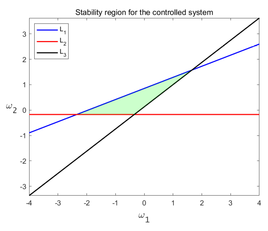
The triangular region surrounded by L 1 ,   L 2 ,   L 3 lines in Equations (37)–(39) accommodates stable eigenvalues.
Proof. 
The marginal stability lines can be obtained from the following conditions:
λ 1 = ± 1 ,   λ 1 λ 2 = 1 .
For the conditions λ 1 λ 2 = 1 , Equation (36) gives
L 1 : J 22 ( J 11 ω 1 ) J 21 ( J 12 ω 2 ) = 1 .
Equation (37) expresses the first condition for marginal stability. For λ 1 = 1 , the Equation (35) yields
L 2 : ω 1 ( 1 J 22 ) + ω 2 J 21 = J 11 + J 22 1 J 11 J 22 + J 21 J 12 .
Similarly for λ 1 = 1 , the following is obtained
L 3 : ω 1 ( 1 + J 22 ) ω 2 J 21 = J 11 + J 22 + 1 + J 11 J 22 J 21 J 12 .
The lines L 1 ,   L 2 ,   L 3 give the conditions for the eigenvalues to have absolute value less than 1. The triangular region surrounded by these line segments gives stable eigenvalues. □

4.2. Hybrid Control Method

The hybrid control method is a strategy for chaos control that combines state feedback and parameter perturbation to stabilize UPO embedded within the chaotic attractor of the system [41]. The collaborative method can ensure that the parameters in the controlled framework can remain stable when the parameters change greatly. By deploying a hybrid control technique, the specific controlled systems are as follows:
S n + 1 = ω S n + ω h λ + b ( 1 I n ) ( μ + p ) S n β 1 β 2 I n η + I n S n I n + n b I n + ( 1 ω ) S n , I n + 1 = ω I n + ω h β 1 β 2 I n η + I n S n I n + m b I n ( α + γ + μ ) I n + ( 1 ω ) I n .
Within this dynamic framework, the parameter ω ( 0 , 1 ) controls chaotic transitions. When an appropriate value of the control parameter ω is chosen, chaos can be delayed or completely eradicated. The Jacobian matrix of system (40) corresponding to E 1 is
J E 1 = 1 + ω h ( μ + p ) β 1 β 2 I η + I I ω h β 1 S ( 2 η + I ) β 2 S I ( η + I ) 2 + n b b ω h β 1 β 2 I η + I I 1 + ω h β 1 S ( 2 η + I ) β 2 S I ( η + I ) 2 + m b ( α + μ + γ ) .
Let
J E 1 = J 11 ω J 12 ω J 21 ω J 22 ω .
Theorem 6. 
The discretized non-linear system (40) is said to be locally asymptotically stable if
1 ( J 11 ω + J 22 ω ) + J 11 ω J 22 ω J 12 ω J 21 ω > 0 ,
1 + ( J 11 ω + J 22 ω ) + J 11 ω J 22 ω J 12 ω J 21 ω > 0 ,
J 11 ω J 22 ω J 12 ω J 21 ω < 0 .
Proof. 
The characteristic equation of (42) gives
F ( λ ) = λ 2 ( J 11 ω + J 22 ω ) + J 11 ω J 22 ω J 12 ω J 21 ω = 0 .
System (40) achieves stability if the zeros of Equation (46) lie in a unit disc. In other words, F ( 1 ) > 0 ,   F ( 1 ) > 0 and F ( 0 ) < 0 . Here,
F ( 1 ) = 1 ( J 11 ω + J 22 ω ) + J 11 ω J 22 ω J 12 ω J 21 ω , F ( 1 ) = 1 + ( J 11 ω + J 22 ω ) + J 11 ω J 22 ω J 12 ω J 21 ω , F ( 0 ) = J 11 ω J 22 ω J 12 ω J 21 ω .
Therefore, system (40) is asymptotically stable under the conditions (43)–(45). □

5. Numerical Simulation

The previous analytical results provide a foundational understanding of the system’s behavior near its equilibrium. To transcend these local insights and explore the global dynamics—including bifurcation sequences, chaotic patterns, and the long-term fate of the disease under various initial conditions—we implement numerical simulations. Specifically, we will examine how variations in the media coverage factor β 2 , the rate of response to the disease under media coverage η , the mortality rate due to the illness α , the rate of recovery γ , the proportion of children born to infected people who are also infected m, the proportion of children born to infected people who are susceptible n.
The equilibrium point E 0 is stable under the conditions of Theorem 1 of (1) in Figure 1. The equilibrium point E 1 is stable under the conditions of Theorem 2 of (1) in Figure 2. From a biological perspective, a stable curve emerges at the disease-free equilibrium E 0 , where media coverage disrupts the disease transmission chain, ultimately achieving disease elimination. Similarly, a stable curve manifests at the endemic equilibrium E 1 . Media influence suppresses the infection rate to minimally acceptable levels, preventing periodic outbreaks and chaotic fluctuations. Conversely, instability in the constant curve at E 1 with increasing h prevents stabilization of susceptible and infected populations, triggering epidemic outbreaks.
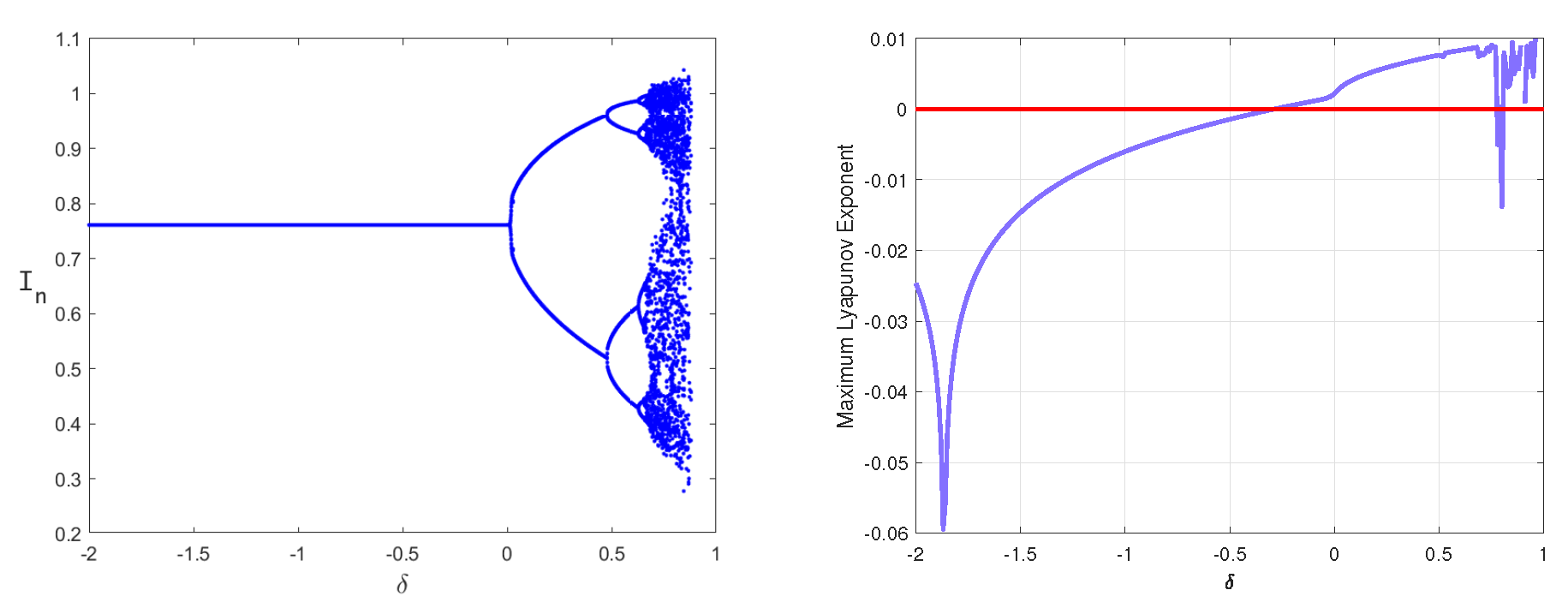
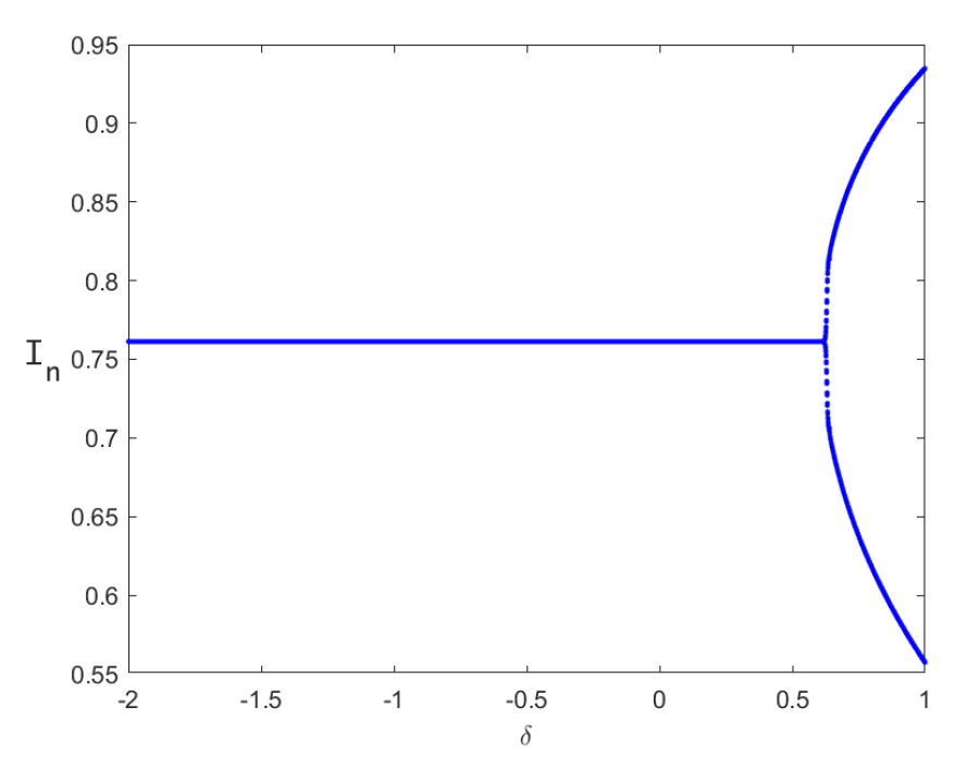
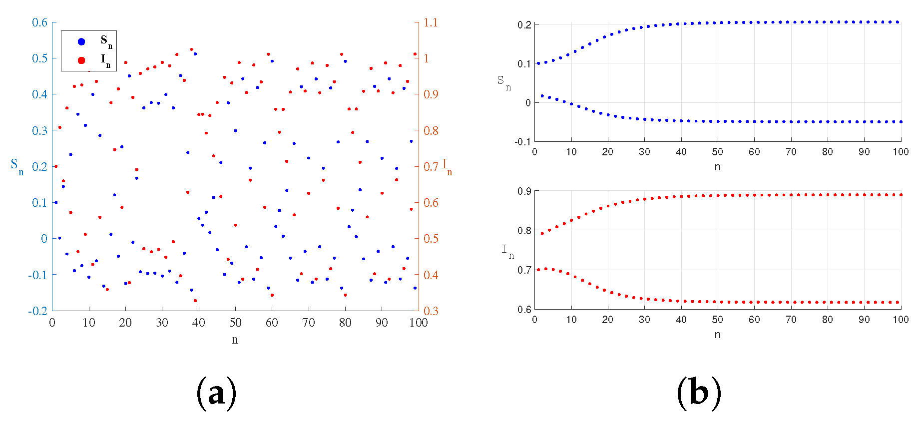
Figure 3 illustrates the periodic solution induced by flip bifurcation at a critical parameter value. Figure 4 presents the bifurcation diagram with the corresponding maximum Lyapunov exponent (MLE), characterizing the system’s transition to chaos. Positive MLE values confirm chaotic dynamics. As perturbation δ varies within ( 0 , 1 ) , the susceptible population I n transitions from period-2 to period-4 oscillations and ultimately to chaotic regimes. Under different media influence factors, the system flip bifurcation occurs. The bifurcation diagram shows that the system dynamics undergo sudden and discontinuous changes, resulting in a sharp outbreak of the epidemic. This inherent unpredictability constitutes a core feature of chaotic dynamics, where disease transmission exhibits sensitivity to minor parameter variations, necessitating precise control to prevent recurrent outbreaks. This creates a core public health challenge: forecasting epidemics becomes highly unreliable in a media-saturated environment. Consequently, control efforts must be agile and adaptive to prevent sharp, unexpected disease resurgences.
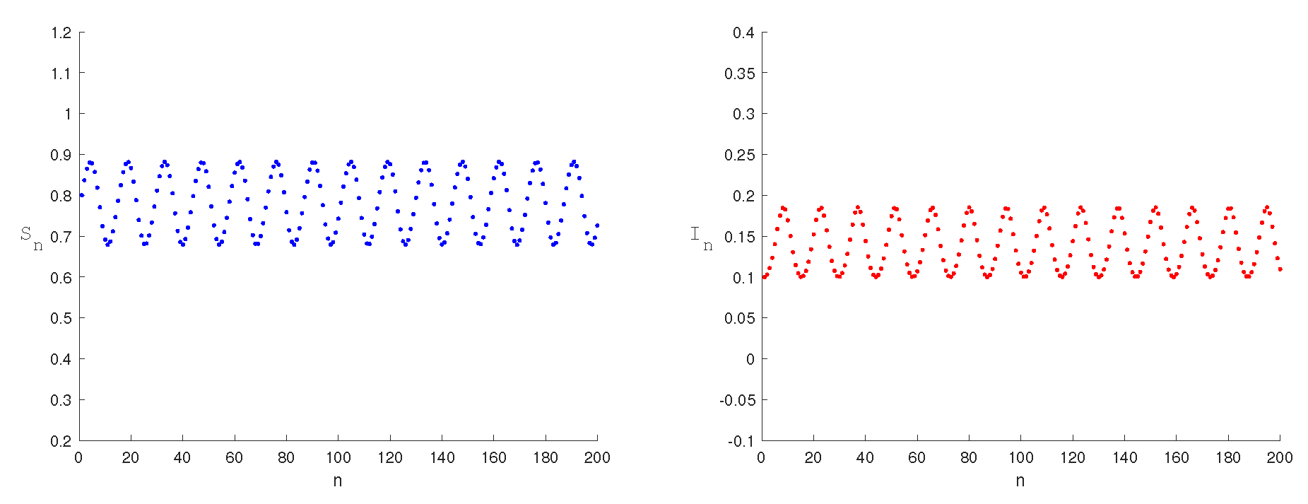
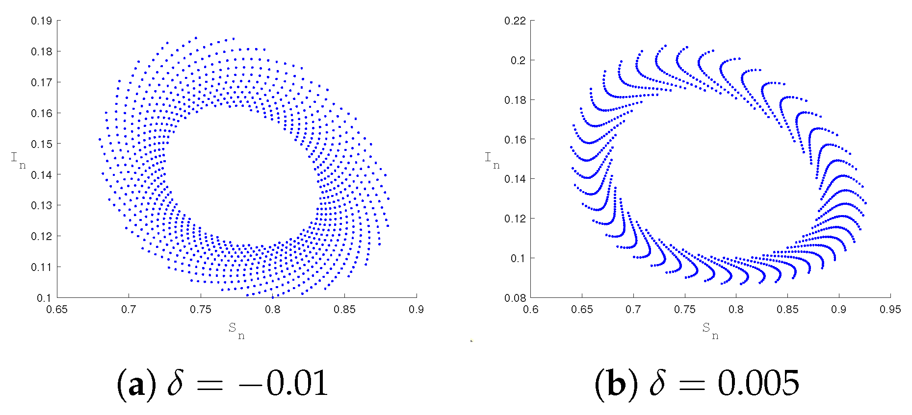
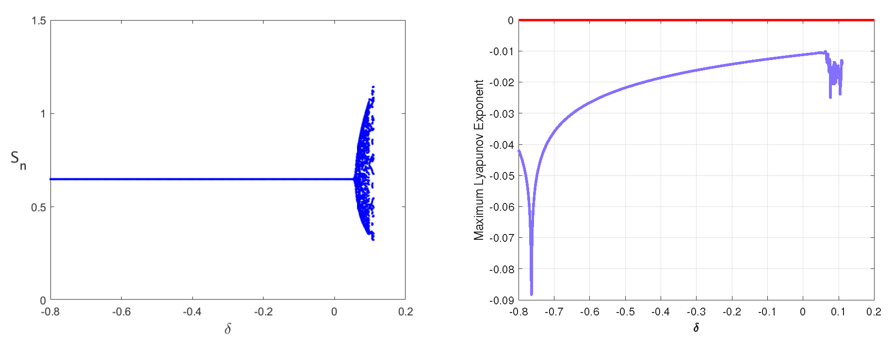
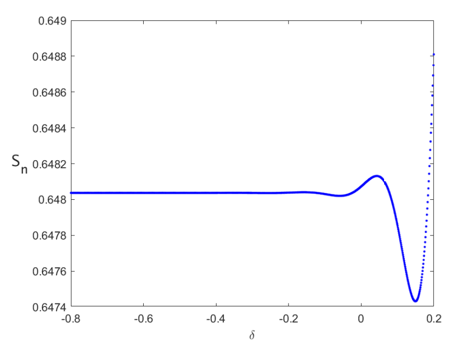
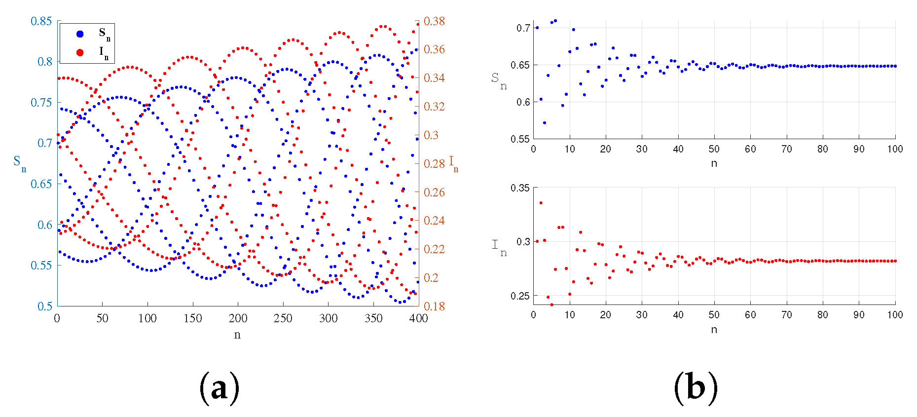
Figure 5 illustrates the periodic solution arising from Neimark–Sacker bifurcation, where the equilibrium transitions from a stable endemic state to quasi-periodic oscillations. This periodic behavior reflects recurrent epidemic fluctuations driven by variations in control efforts. Figure 6 displays phase portraits under different perturbations, revealing trajectory evolution; meanwhile, Figure 7 presents the Neimark–Sacker bifurcation diagram alongside its corresponding maximum Lyapunov exponent. Figure 5 is the wave diagram, and Figure 6 is the corresponding closed curve diagram. The bifurcation occurs at critical δ values ( 0.06 δ 0.12 ), manifesting as a closed ring or dense point cloud in the number of susceptible population S n . Increasing δ from 0.01 to 0.005 transitions disease dynamics from recoverable stability to sustained complex oscillations. Heightened media coverage induces behavioral changes, such as increased voluntary social distancing. These changes are strong enough to disrupt steady transmission yet insufficient to eliminate the disease, ultimately leading to recurrent epidemic waves. Under different media influence factors, the system flip bifurcation occurs. The bifurcation diagram shows that the disease epidemic has a persistent oscillation or seasonal epidemic. It indicates that the influence of media reports drives the repeated transmission cycle of the disease. These findings establish theoretical foundations for public health policy design.
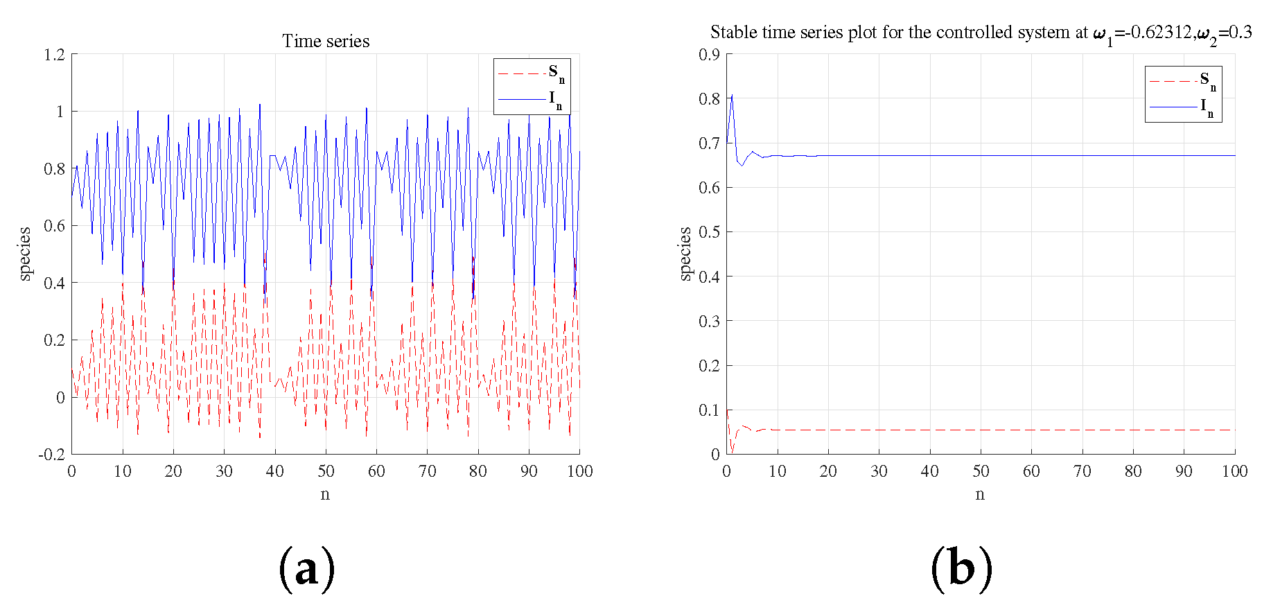
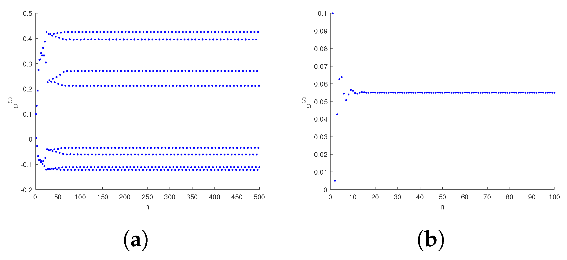
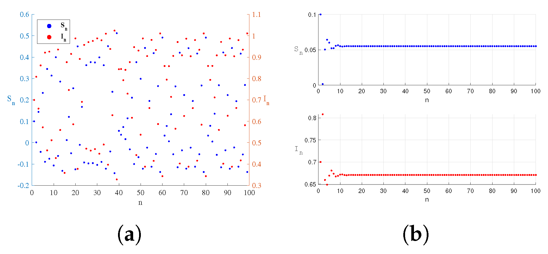
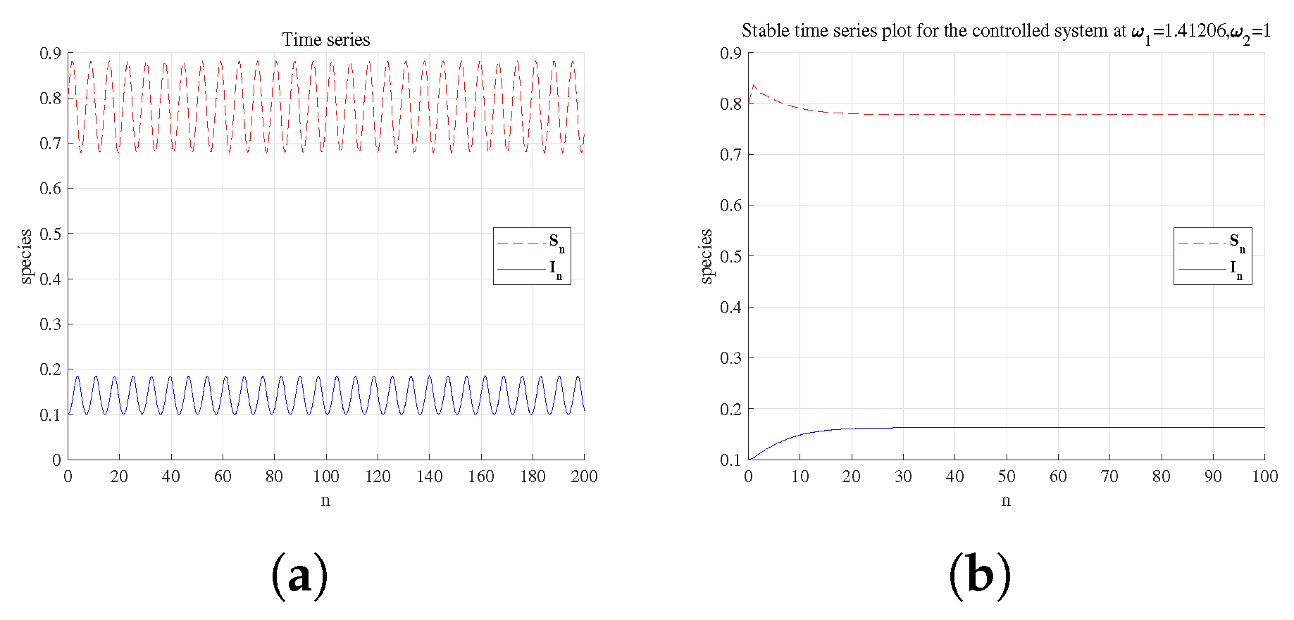
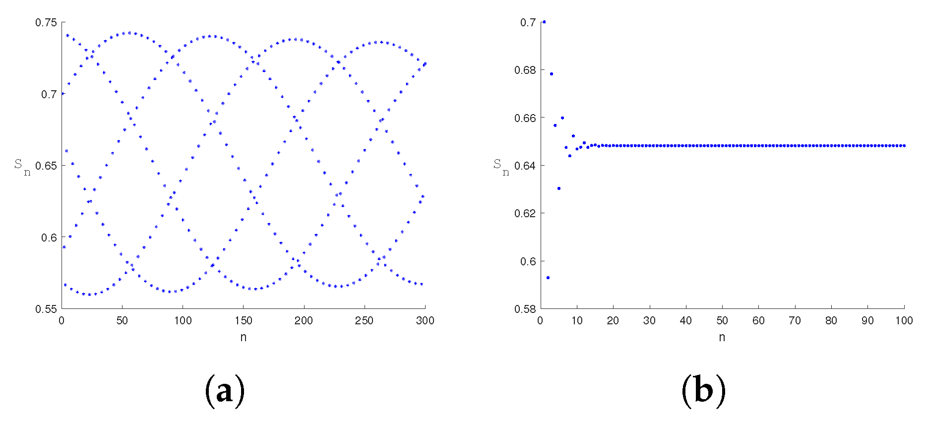
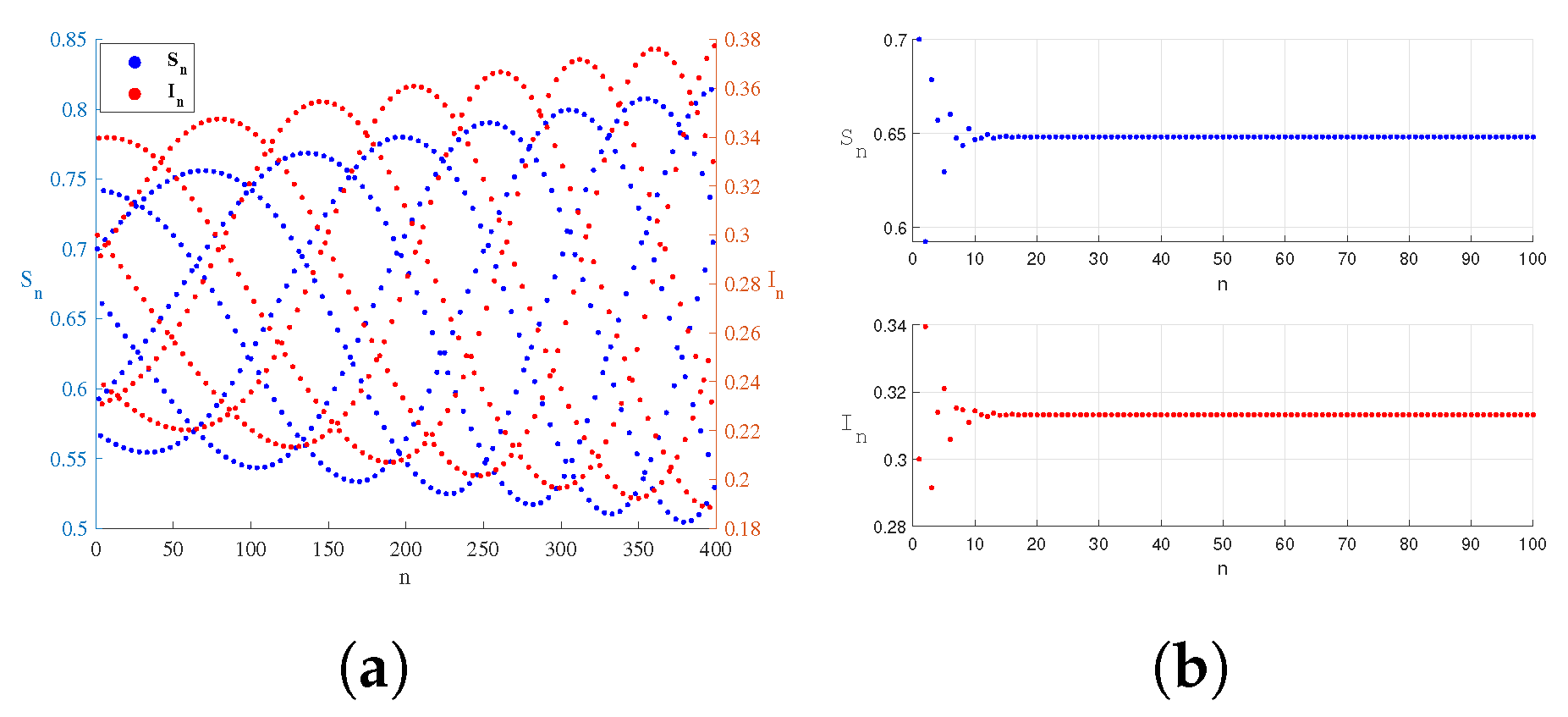
Figure 8, Figure 9, Figure 10, Figure 11, Figure 12, Figure 13, Figure 14 and Figure 15 show that system (32) controls flip and Neimark–Sacker bifurcations under different parameter conditions. For flip bifurcation, the state feedback control method considers the following set of parameters: β 1 = 0.9 ,   β 2 = 0.09 ,   h = 3.44338 , λ = 0.03 ,   μ = 0.008 ,   α = 0.002 ,   γ = 0.04 ,   p = 0.009 ,   b = 0.009 ,   m = 0.6 ,   n = 0.4 , η = 0.003 . For Neimark–Sacker bifurcation, the state feedback control method considers the following set of parameters: β 1 = 0.9 ,   β 2 = 0.1 ,   h = 3.15947 ,   λ = 0.1 ,   μ = 0.2 , α = 0.3 ,   γ = 0.1 , p = 0.002 ,   b = 0.2 ,   m = 0.4 ,   n = 0.6 ,   η = 0.007 . Figure 8 and Figure 12 depict that the controlled system (32) is stable in the green triangle region under certain parameters and reveals the critical condition of bifurcation. The green stable region represents the parameter space where the control strategy is effective and can maintain the disease in a stable and controllable state. The time-series in Figure 9, Figure 10, Figure 11 and Figure 13, Figure 14, Figure 15 show that the application of specific feedback gains ( ω 1 , ω 2 ) can effectively regulate the system from a destabilized state (e.g., cyclic oscillation or chaos) to a stable equilibrium. The time series in Figure 9, Figure 10, Figure 11 and Figure 13, Figure 14, Figure 15 confirm that specific feedback gains ( ω 1 , ω 2 ) effectively transition the system from destabilized states (e.g., limit cycles or chaos) to stable equilibriums. Specifically, bifurcation diagrams in Figure 9, Figure 10, Figure 11 show period-8 oscillations and chaotic attractors converging to stability, while Figure 13, Figure 14, Figure 15 exhibit limit cycles converging to stable regimes. Strategic adjustment of media coverage intensity and feedback gains suppresses epidemic outbreaks and recurrences, providing theoretical foundations for dynamic prevention strategies.
For the hybrid control method, Figure 16, Figure 17, Figure 18, Figure 19 further demonstrate that the variation in the control parameter ω in system (40) induces the dynamic evolution of the system state variables S n and I n , verifying the robustness of the control strategy. For flip bifurcation, the hybrid control method considers the following set of parameters: β 1 = 0.9 ,   β 2 = 0.09 , h = 3.44338 ,   λ = 0.03 ,   μ = 0.008 ,   α = 0.002 ,   γ = 0.04 ,   p = 0.009 ,   b = 0.009 ,   m = 0.6 , n = 0.4 ,   η = 0.003 . For Neimark–Sacker bifurcation, the hybrid control method considers the following set of parameters: β 1 = 0.9 ,   β 2 = 0.1 ,   h = 3.15947 ,   λ = 0.1 , μ = 0.2 ,   α = 0.3 ,   γ = 0.1 ,   p = 0.002 ,   b = 0.2 ,   m = 0.4 ,   n = 0.6 ,   η = 0.007 . In the bifurcation diagrams of these values shown in Figure 17 and Figure 19, the system chaos and limit cycle phenomenon converge to the stable window. Adjusting this parameter is equivalent to strengthening public health measures such as media reporting, which suppresses bifurcation phenomena and transitions the infectious disease system from an unstable (outbreak) state to a stable (controlled) state. This transition provides a theoretical basis for formulating dynamic adaptive prevention strategies. Implementation involves intensifying media coverage through major platforms by disseminating infection sources, transmission routes, case counts, and patient trajectories (as demonstrated during COVID-19). These interventions effectively combat epidemics.
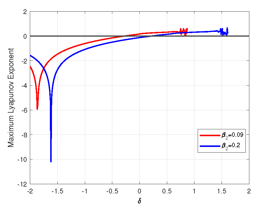
Figure 20 represents the maximum Lyapunov exponent when system 3 changes only the value of the media coverage impact factor take and flip bifurcation occurs at equilibrium E 1 . The set of parameters taken is as follows: β 1 = 0.9 , h = 3.44338 ,   λ = 0.03 ,   μ = 0.008 , α = 0.002 ,   γ = 0.04 ,   p = 0.009 ,   b = 0.009 ,   m = 0.6 ,   n = 0.4 ,   η = 0.003 . Numerical simulations indicate that a lower media impact factor ( β 2 = 0.09 ) leads to an earlier onset of chaotic dynamics compared to a higher value ( β 2 = 0.2 ). These results demonstrate that sustained, high-impact media coverage acts as a stabilizing force, delaying or preventing the transition to chaotic disease spread. Conversely, inadequate media attention leads to prematurely chaotic dynamics, characterized by sudden and unpredictable epidemic resurgences that are difficult to manage. This underscores the critical role of strategic risk communication as a non-pharmaceutical intervention to mitigate outbreak unpredictability. These results underscore the potential of strategically managing media coverage as an effective intervention for mitigating and controlling infectious disease outbreaks.

6. Conclusions

In this paper, we have explored a discrete epidemic model affected by media coverage. We have developed a discrete epidemic model and analyzed the local stability and instability conditions associated with two equilibrium points within system (3). We have characterized the flip bifurcation at the positive equilibrium point, identifying critical thresholds λ = 1 through coefficient analysis. Furthermore, we have investigated the Neimark–Sacker bifurcation, which arises when the eigenvalues form a pair of conjugate complex roots | λ 1 |   =   | λ 2 |   =   1 .
We have derived and controlled chaotic dynamics through state feedback control and hybrid control methods to stabilize bifurcation-induced instability. The chaotic behavior of the system has been studied theoretically. We have proved that chaos and limit cycle phenomena can be controlled by state feedback control and hybrid control methods. By adjusting the parameters, the bifurcation diagram obviously changes from chaotic attractors and limit cycles to stable solutions. The above numerical simulation has verified the occurrence of bifurcation and chaos in the system.
Our findings have shown that media coverage can regulate the intensity of the outbreak and expand the chaotic mechanism, which can effectively prevent the large-scale outbreak of infectious diseases through control. From a biological point of view, the stability analysis of the equilibrium point has demonstrated that under the influence of media reports, the local equilibrium infection rate is suppressed to the lowest acceptable level to avoid periodic outbreaks or chaotic fluctuations. By controlling the chaos and limit cycles caused by flip bifurcation and Neimark–Sacker bifurcation, we have confirmed that disease transmission dynamics can be effectively suppressed. This suppression is achieved by strengthening media coverage and disseminating key information including source of infection, route of transmission, number of cases, and patient trajectory through major media platforms. These interventions have proven effective in epidemic containment.
Although prior works have integrated media effects into epidemic models, they are predominantly confined to continuous-time dynamics. However, the field has neglected a comprehensive interdisciplinary investigation that bridges media coverage with discrete modeling and bifurcation theory. This article addresses this gap by constructing a more realistic discrete model of media influence and establishing a corresponding bifurcation analysis framework tailored to this model. The Euler discrete method proposed in this paper shows higher computational efficiency. When the same solution accuracy is achieved, the calculation time and strength are greatly reduced. At the same time, it also has rich dynamic properties, which reduces the threshold of practical application. Therefore, it provides an efficient, stable, and practical tool for solving discrete and bifurcation problems. These results have demonstrated that the dynamic behavior of the discrete model is more complex. Consequently, discrete epidemic modeling has emerged as a significant direction for future research.

Author Contributions

Writing—original draft, Y.L.; Conceptualization, Y.L. and W.W.; Visualization, Y.L. and W.W.; Writing—review and editing, Y.L. and W.W. All authors have read and agreed to the published version of the manuscript.

Funding

This research was funded the Fundamental Research Funds for the Central Universities (Grant No. 2572022DJ04).

Institutional Review Board Statement

Not applicable.

Informed Consent Statement

Not applicable.

Data Availability Statement

The original contributions presented in the study are included in the article; further inquiries can be directed to the corresponding author.

Conflicts of Interest

The authors declare no conflicts of interest.

References

  1. Gumel, A.B.; Ruan, S.; Day, T.; Watmough, J.; Brauer, F.; Van den, P.; Gabrielson, D.; Bowman, C.; Alexander, M.E.; Ardal, S.; et al. Modelling strategies for controlling SARS outbreaks. Proc. R. Soc. Lond. B 2004, 271, 2223–2232. [Google Scholar] [CrossRef] [PubMed]
  2. Premkumar, M.; Devurgowda, D.; Dudha, S.; Maiwall, R.; Bihari, C.; Grover, S.; Gupta, E.; Kumar, S.; Sarin, S.K. A/H1N1/09 Influenza is Associated With High Mortality in Liver Cirrhosis. Clin. Exp. Hepatol. 2019, 9, 162–170. [Google Scholar] [CrossRef]
  3. Yıldırım, M.; Solmaz, F. COVID-19 burnout, COVID-19 stress and resilience: Initial psychometric properties of COVID-19 Burnout Scale. Death Stud 2020, 46, 524–532. [Google Scholar] [CrossRef] [PubMed]
  4. Deng, J.; Tang, S.; Shu, H. Joint impacts of media, vaccination and treatment on an epidemic Filippov model with application to COVID-19. J. Theor. Biol. 2021, 523, 110698. [Google Scholar] [CrossRef]
  5. Miller, E. Rapid evaluation of the safety of COVID-19 vaccines: How well have we done? Clin. Microbiol. Infect. 2022, 28, 477–478. [Google Scholar] [CrossRef]
  6. Shoaib, M.; Kainat, S.; Alabduljabbar, A.A.; Nisar, K.S.; Zahoor Raja, M.A. Integrated intelligent neuro-evolutionary computing approach to study SEIRC model representing campylobacteriosis transmission dynamics. Appl. Math. Sci. Eng. 2024, 33, 2441257. [Google Scholar] [CrossRef]
  7. Waqar, M.; Khan, Z.A.; Khawaja, S.T.; Chaudhary, N.I.; Khan, S.; Cheema, K.M.; Khan, M.F.; Ahmed, S.S.; Raja, M.A.Z. Explainable clinical diagnosis through unexploited yet optimized fine-tuned ConvNeXt models for accurate monkeypox disease classification. SLAS Technol. 2025, 33, 100336. [Google Scholar] [CrossRef] [PubMed]
  8. Phua, K.L.; Lee, L. Meeting the Challenge of Epidemic Infectious Disease Outbreaks: An Agenda for Research. J. Public Health Pol. 2005, 26, 122–132. [Google Scholar] [CrossRef]
  9. Mustafa, N.; Rahman, J.U.; Omame, A. Modelling of Marburg virus transmission dynamics: A deep learning-driven approach with the effect of quarantine and health awareness interventions. Model. Earth Syst. Environ. 2024, 10, 7337–7357. [Google Scholar] [CrossRef]
  10. Mannan, A.; Shoket, N.; Ul Rahman, J.; Uwitije, R. Dynamic analysis of ebola virus disease with non-linear incidence rate using morlet wavelet neural networks and hybrid optimization techniques. Model. Earth Syst. Environ. 2025, 11, 79. [Google Scholar] [CrossRef]
  11. Misra, A.K.; Sharma, A.; Shukla, J.B. Modeling and analysis of effects of awareness programs by media on the spread of infectious diseases. Math. Comput. Model. 2011, 53, 1221–1228. [Google Scholar] [CrossRef]
  12. Tchuenche, J.M.; Dube, N.; Bhunu, C.P.; Smith, R.J.; Bauch, C.T. The impact of media coverage on the transmission dynamics of human influenza. BMC Public Health 2011, 11, S5. [Google Scholar] [CrossRef]
  13. Sahu, G.P.; Dhar, J. Dynamics of an SEQIHRS epidemic model with media coverage, quarantine and isolation in a community with pre-existing immunity. J. Math. Anal. Appl. 2015, 421, 1651–1672. [Google Scholar] [CrossRef]
  14. Yan, Q.; Tang, S.; Gabriele, S.; Wu, J. Media coverage and hospital notifications: Correlation analysis and optimal media impact duration to manage a pandemic. J. Theor. Biol. 2016, 390, 1–13. [Google Scholar] [CrossRef]
  15. Zhou, W.; Xiao, Y.; Heffernan, J.M. Optimal media reporting intensity on mitigating spread of an emerging infectious disease. PLo1S ONE 2019, 14, e0213898. [Google Scholar] [CrossRef]
  16. Bitrus, K.; Abdullah, F.A.; Adewole, M.O. Uncovering the influence of public awareness on dengue population dynamics: A mathematical model approach. Bol. Soc. Mat. Mex. 2025, 31, 86. [Google Scholar] [CrossRef]
  17. Sun, Z.; Zhang, H.; Yang, Y.; Wan, H.; Wang, Y. Impacts of geographic factors and population density on the COVID-19 spreading under the lockdown policies of China. Sci. Total Environ. 2020, 746, 141347. [Google Scholar] [CrossRef]
  18. Kahn, R.; Holmdahl, I.; Reddy, S.; Jernigan, J.; Mina, M.J.; Slayto, R.B. Mathematical Modeling to Inform Vaccination Strategies and Testing Approaches for Coronavirus Disease 2019 (COVID-19) in Nursing Homes. Clin. Microbiol. Infect. 2022, 74, 597–603. [Google Scholar] [CrossRef] [PubMed]
  19. Das, D.K.; Khajanchi, S.; Kar, T.K. The impact of the media awareness and optimal strategy on the prevalence of tuberculosis. Appl. Math. Comput. 2020, 366, 124732. [Google Scholar] [CrossRef]
  20. Liu, P.; Luo, Y.; Teng, Z. Role of media coverage in a SVEIR-I epidemic model with nonlinear incidence and spatial heterogeneous environment. Math. Biosci. Eng. 2023, 20, 15641–15671. [Google Scholar] [CrossRef] [PubMed]
  21. Liu, J.; Peng, B.; Zhang, T. Effect of discretization on dynamical behavior of SEIR and SIR models with nonlinear incidence. Appl. Math. Lett. 2015, 39, 60–66. [Google Scholar] [CrossRef]
  22. Qin, W.; Zhang, J.; Dong, Z. Media impact research: A discrete SIR epidemic model with threshold switching and nonlinear infection forces. Math. Biosci. Eng. 2023, 20, 17783–17802. [Google Scholar] [CrossRef]
  23. Zhu, L.; Wang, X.; Zhang, H.; Shen, S.; Li, Y.; Zhou, Y. Dynamics analysis and optimal control strategy for a SIRS epidemic model with two discrete time delays. Phys. Scr. 2020, 95, 035213. [Google Scholar] [CrossRef]
  24. Zhang, T.; Liu, J.; Teng, Z. Threshold conditions for a discrete nonautonomous SIRS model. Math. Methods Appl. Sci. 2015, 38, 1781–1794. [Google Scholar] [CrossRef]
  25. van den Driessche, P.; Yakubu, A.A. Disease Extinction Versus Persistence in Discrete-Time Epidemic Models. Bull. Math. Biol. 2019, 81, 4412–4446. [Google Scholar] [CrossRef] [PubMed]
  26. Cao, H.; Zhou, Y.; Ma, Z. Bifurcation analysis of a discrete SIS model with bilinear incidence depending on new infection. Math. Biosci. Eng. 2013, 10, 1399–1417. [Google Scholar] [CrossRef] [PubMed]
  27. Peng, M. Bifurcation and chaotic behavior in the Euler method for a Uçar prototype delay model. Chaos Solitons Fractals 2004, 22, 483–493. [Google Scholar] [CrossRef]
  28. Anguelov, R.; Dukuza, K.; Lubuma, J.M.S. Backward bifurcation analysis for two continuous and discrete epidemiological models. Math. Methods Appl. Sci. 2018, 41, 8784–8798. [Google Scholar] [CrossRef]
  29. Yu, X.; Liu, M.; Zheng, Z.; Hu, D. Complex dynamics of a discrete-time SIR model with nonlinear incidence and recovery rates. Int. J. Biomath. 2023, 16, 2250131. [Google Scholar] [CrossRef]
  30. Arenas, A.; Garijo, A.; Gómez, S.; Villadelprat, J. Bifurcation analysis of the Microscopic Markov Chain Approach to contact-based epidemic spreading in networks. Chaos Solitons Fractals 2023, 166, 112921. [Google Scholar] [CrossRef]
  31. Zhang, X.; Zhang, C.; Zhang, Y. Pattern dynamics analysis of a time-space discrete FitzHugh-Nagumo (FHN) model based on coupled map lattices. Comput. Math. Appl. 2024, 157, 92–123. [Google Scholar] [CrossRef]
  32. Wu, G.C.; Baleanu, D. Discrete chaos in fractional delayed logistic maps. Nonlinear Dyn. 2015, 80, 1697–1703. [Google Scholar] [CrossRef]
  33. Li, Y.; Rafaqat, M.; Zia, T.J.; Ahmed, I.; Jung, C.Y. Flip and Neimark-Sacker Bifurcations of a Discrete Time Predator-Prey Model. IEEE Access 2019, 7, 123430–123435. [Google Scholar] [CrossRef]
  34. Chen, X.; Yuan, S.; Jing, Z.; Fu, X. Bifurcation and Chaos of a Discrete-Time Mathematical Model for Tissue Inflammation. J. Dyn. Diff. Equat. 2016, 28, 281–299. [Google Scholar] [CrossRef]
  35. Singh, A.; Deolia, P. Bifurcation and Chaos in a Discrete Predator–Prey Model with Holling Type-III functional Response and harvesting Effect. J. Biol. Syst. 2021, 29, 451–478. [Google Scholar] [CrossRef]
  36. Chakraborty, K. Ecological complexity and feedback control in a prey–predator system with Holling type III functional response. COMPLEXITY 2016, 21, 346–360. [Google Scholar] [CrossRef]
  37. Auerbach, D.; Grebogi, C.; Ott, E.; Yorke, J.A. Controlling chaos in high dimensional systems. Phys. Rev. Lett. 1992, 69, 3479–3482. [Google Scholar] [CrossRef]
  38. Luo, X.S.; Chen, G.; Wang, B.H.; Fang, J.Q. Hybrid control of period-doubling bifurcation and chaos in discrete nonlinear dynamical systems. Chaos Solitons Fractals 2003, 18, 775–783. [Google Scholar] [CrossRef]
  39. Elaydi, S.N. Discrete Chaos; Chapman & Hall/CRC: Boca Raton, FL, USA, 2007. [Google Scholar]
  40. Din, Q. Complexity and chaos control in a discrete-time prey-predator model. Commun. Nonlinear Sci. Numer. Simul. 2017, 49, 113–134. [Google Scholar] [CrossRef]
  41. Yuan, L.G.; Yang, Q.G. Bifurcation, invariant curve and hybrid control in a discrete-time predator–prey system. Appl. Math. Model. 2015, 39, 2345–2362. [Google Scholar] [CrossRef]
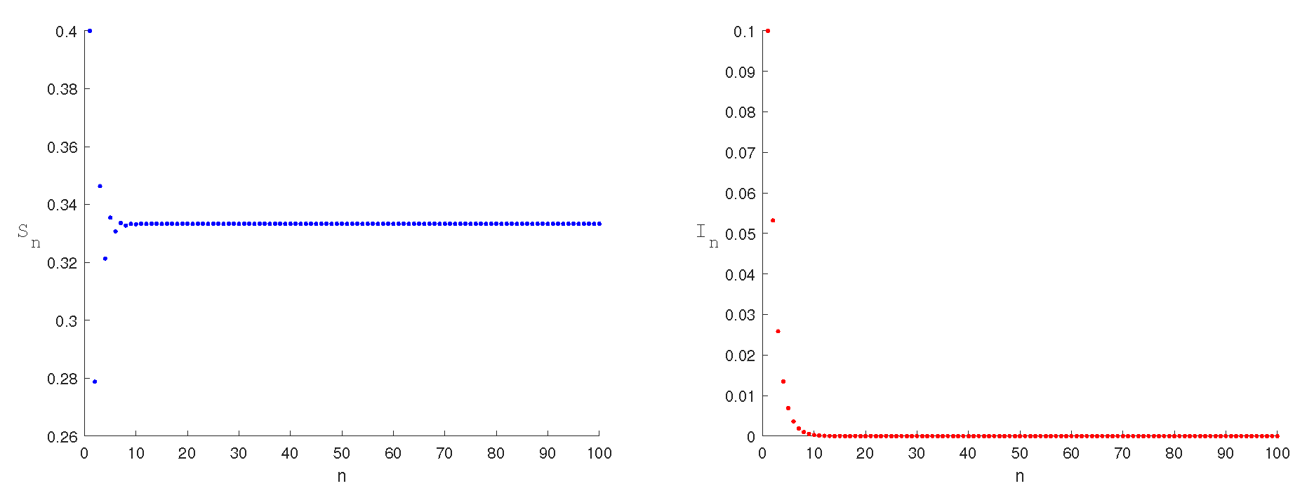
Figure 1. The equilibrium point E 0 is stable when the parameter β 1 = 0.4 ,   β 2 = 0.1 ,   h = 1.2 ,   λ = 0.3 , μ = 0.4 ,   α = 0.1 ,   γ = 0.1 ,   p = 0.8 ,   b = 0.1 ,   m = 0.7 ,   n = 0.3 ,   η = 0.1 , and the initial value is (0.4,0.1).
Axioms 14 00681 g001
Figure 2. The equilibrium point E 1 is stable when the parameter β 1 = 0.8 ,   β 2 = 0.1 ,   h = 1.1 , λ = 0.06 ,   μ = 0.8 ,   α = 0.1 ,   γ = 0.1 ,   p = 0.3 ,   b = 0.9 ,   m = 0.6 ,   n = 0.4 ,   η = 0.1 , and the initial value is (0.63235,0.26441).
Axioms 14 00681 g002
Figure 3. Flip bifurcation periodic solution at E 1 . Take the value of the parameter β 1 = 0.9 , β 2 = 0.01 ,   h = 1.44929 ,   λ = 0.06 ,   μ = 0.004 ,   α = 0.03 ,   γ = 0.01 ,   p = 0.8 ,   b = 0.005 ,   m = 0.9 , n = 0.1 ,   η = 0.1 , and the initial value is (0.01152,0.37189).
Axioms 14 00681 g003
Figure 4. Bifurcation of system (3) in ( δ , I n ) plane Maximal Lyapunov exponent for β 1 = 0.9 , β 2 = 0.09 ,   h = 3.44338 ,   λ = 0.03 ,   μ = 0.008 ,   α = 0.002 ,   γ = 0.04 ,   p = 0.009 ,   b = 0.009 ,   m = 0.6 , n = 0.4 ,   η = 0.003 at E 1 .
Axioms 14 00681 g004
Figure 5. Neimark–Sacker bifurcation periodic solution at E 1 . Take the values of the parameters as β 1 = 0.9 ,   β 2 = 0.001 ,   h = 1.46724 ,   λ = 0.002 ,   μ = 0.004 ,   α = 0.006 ,   γ = 0.7 ,   p = 0.001 ,   b = 0.1 , m = 0.1 ,   n = 0.9 ,   η = 0.1 , and the initial value is (0.46681,0.51831).
Axioms 14 00681 g005
Figure 6. Phase diagram of the equilibrium point E 1 = ( 0.46681 , 0.51831 ) under different perturbations (a) δ = 0.01 , (b) δ = 0.005 , when the parameters take the values β 1 = 0.9 ,   β 2 = 0.001 , h = 1.46724 ,   λ = 0.002 ,   μ = 0.004 ,   α = 0.006 ,   γ = 0.7 ,   p = 0.001 ,   b = 0.1 ,   m = 0.1 ,   n = 0.9 ,   η = 0.1 .
Axioms 14 00681 g006
Figure 7. Bifurcation of system (3) in ( δ , S n ) plane and Maximal Lyapunov exponent for β 1 = 0.9 , β 2 = 0.1 , h = 3.15947 ,   λ = 0.1 ,   μ = 0.2 ,   α = 0.3 ,   γ = 0.1 ,   p = 0.002 ,   b = 0.2 ,   m = 0.4 ,   n = 0.6 , η = 0.007 at E 1 .
Axioms 14 00681 g007
Figure 8. Stability region for the controlled system (32) when flip bifurcation occurs.
Axioms 14 00681 g008
Figure 9. A time- series is drawn for flip bifurcation. Taking feedback gains ω 1 = 0.623116 ,   ω 2 = 0.3 , the system changes from unstable (a) to stable (b).
Axioms 14 00681 g009
Figure 10. Taking the values of parameters δ = 0.65 ,   ω 1 = 0.623116 ,   ω 2 = 0.3 , the S n changes with time during flip bifurcation. The system changes from unstable (a) to stable (b).
Axioms 14 00681 g010
Figure 11. Taking the values of parameters δ = 0.8 ,   ω 1 = 0.623116 ,   ω 2 = 0.3 , the S n ,   I n changes with time during flip bifurcation. The system changes from unstable (a) to stable (b).
Axioms 14 00681 g011
Figure 12. Stability region for the U+2212 controlled system (32) when Neimark–Sacker bifurcation occurs.
Axioms 14 00681 g012
Figure 13. A time-series is drawn for Neimark–Sacker bifurcation. Taking feedback gains ω 1 = 1.41206 ,   ω 2 = 1 , the system changes from unstable (a) to stable (b).
Axioms 14 00681 g013
Figure 14. Taking the values of parameters δ = 0.06 ,   ω 1 = 1.41206 ,   ω 2 = 1 , the S n changes with time during Neimark–Sacker bifurcation. The system changes from unstable (a) to stable (b).
Axioms 14 00681 g014
Figure 15. Taking the values of parameters δ = 0.07 ,   ω 1 = 1.41206 ,   ω 2 = 1 , the S n ,   I n changes with time during Neimark–Sacker bifurcation. The system changes from unstable (a) to stable (b).
Axioms 14 00681 g015
Figure 16. Flip bifurcation diagram with respect to δ for system (40) with ω = 0.85 .
Axioms 14 00681 g016
Figure 17. Taking the values of parameters δ = 0.8 ,   ω = 0.85 , the S n ,   I n changes with time during flip bifurcation. The system changes from unstable (a) to stable (b).
Axioms 14 00681 g017
Figure 18. Neimark–Sacker bifurcation diagram with respect to δ for system (40) with ω = 0.9 .
Axioms 14 00681 g018
Figure 19. Taking the values of parameters δ = 0.07 ,   ω = 0.9 , the S n ,   I n changes with time during Neimark–Sacker bifurcation. The system changes from unstable (a) to stable (b).
Axioms 14 00681 g019
Figure 20. Maximal Lyapunov exponent at E 1 .
Axioms 14 00681 g020
Disclaimer/Publisher’s Note: The statements, opinions and data contained in all publications are solely those of the individual author(s) and contributor(s) and not of MDPI and/or the editor(s). MDPI and/or the editor(s) disclaim responsibility for any injury to people or property resulting from any ideas, methods, instructions or products referred to in the content.