Analysis of Bifurcation and Stability in an Epidemic Model of HPV Infection and Cervical Cancer with Two Time Delays

Abstract

Cervical cancer (CC), which continues to be a major public health concern that causes cancer deaths among women worldwide, is mostly caused by persistent human papillomavirus (HPV) infection. This study suggests a dual-delay model of HPV-C infection dynamics that takes into account both cancerous delay and the immune response delay. We identify disease-free and diseased equilibria, investigate their local asymptotic stability, and show that the system is non-negative and bounded. We prove the global asymptotic stability of the equilibria by building Lyapunov functions and using the basic reproduction number $R_0$, and look into the existence of Hopf bifurcations. Additionally, we use forward sensitivity analysis to determine important control parameters. Lastly, the theoretical results were confirmed by numerical simulations. The study demonstrates that time delays play a crucial role in viral transmission and carcinogenesis. The process from HPV infection to the formation of cervical cancer is more correctly simulated by this model, which offers a theoretical mathematical basis for researching the pathophysiology of cervical cancer and developing clinical prevention and control measures.

1. Introduction

The human papillomavirus, or HPV, is one of the most prevalent sexually transmitted diseases (STDs) in the world. There are more than 200 subtypes of HPV, and the World Health Organization (WHO) has defined at least 14 of them as high-risk. These include HPV-16 and HPV-18, and they are strongly linked to the pathophysiology of several malignant tumors, such as anal and cervical cancer (CC) [1]. The WHO has released statistics showing that CC is the fourth most common cancer in women globally, with around 660,000 new cases and around 350,000 deaths in 2022 [2]. Research indicates that HPV infection is closely associated with the development of CC, with persistent infection by high-risk HPV (HR-HPV) serving as a critical factor in the induction of precancerous lesions and CC. Therefore, comprehending the transmission dynamics of HPV infection and its pathological mechanisms in the progression of CC remains an essential issue to be addressed within the realm of public health [3,4].

For this reason, many researchers have studied HPV in great detail and developed a number of mathematical models to explain how it spreads and to find efficient ways to avoid it [5,6,7,8], including some fractional-order models of co-infection with other illnesses [9,10]. By providing more sophisticated instruments for examining the intricate relationships present in multi-disease co-infection situations linked to HPV, we advance our knowledge of co-infection phenomena.

However, three primary phases are usually identified in the lengthy and complicated process of HPV infection leading to CC: persistent HPV infection, cervical intraepithelial neoplasia (CIN), and finally, invasive CC [11]. The dynamics of HPV transmission present two clear biological features. First, there is a delay between the post-infection of the virus and viral clearance; and second, cervical carcinogenesis is a multi-stage process that usually takes 10–30 years to progress from persistent HPV infection to CIN and ultimately to invasive carcinoma [12]. We refer to it as the carcinogenic latency period. Due to these time-scale heterogeneities, it may be challenging to accurately depict the dynamic relationship using conventional ordinary differential equation (ODE) models. Thus, the incorporation of time delays into mathematical models has become crucial to improving the models’ biological plausibility.

Multiple studies have actually created and examined delay models for HPV infectious disease, taking into account different kinds of delays such as immune response, recovery, and incubation period delays. Time delays in the dynamics of HPV and CC cells were included in a model created by Akimenko et al. [13], highlighting the necessity of prompt actions to stop the evolution of the disease. Some researchers have thought about how treatment delays affect HPV transmission dynamics. For example, according to Goel et al. [14], treatment delays had a major effect on oropharyngeal cancer survival rates; the longer the time between diagnosis and surgery, the worse the result, especially in HPV negative cases. In contrast, Vasudev et al. [15] found that treatment delays had no discernible effect on survival in patients with HPV OPSCC, implying that time may have an impact on treatment outcomes depending on HPV status.

Even though the effects of time delays on system dynamics have been studied before, real-world complex systems frequently feature processes where several time delays interact at once. Thus, it will be more realistic to show the dynamic features of processes like illness progression if the synergistic impacts of various time delays on system behavior are taken into account. To the best of our knowledge, no research has examined the effects of cancerous delay and the immune response delay in the development of CC from HPV infection.

Based on this, we examined the effects of the cancerous delay and the immune response delay on an HPV and CC (HPV-C) system for the first time. Meanwhile, we also examine the stability of the system, the occurrence of Hopf bifurcation, etc. The article has the following structure: Section 2 gives a delay differential equation (DDE) system of HPV transmission and CC. The Section 3 examines the non-negativity, boundedness, and existence of solutions. The Section 4 examines the stability of the equilibrium point of the system and examines whether a Hopf bifurcation exists. In the Section 5, the focus shifts to analyzing the nature of the Hopf bifurcation, specifically analyzing its directionality and stability. Section 6 verifies the results through numerical simulation. In the last section, we summarize the entire paper.

2. Model Formulation

Rajan et al. [16] used a compartmental epidemiological paradigm to systematically investigate the multistage pathogenesis from HPV infection to cervical carcinogenesis. The female population $N\left(t\right)$ is divided into four different epidemiological divisions:

$$N\left(t\right)=S\left(t\right)+I\left(t\right)+C\left(t\right)+R\left(t\right),$$

(1)

where $S\left(t\right)$ represents the susceptible population, which consists of uninfected people; $I\left(t\right)$ stands for asymptomatic HPV carriers; $C\left(t\right)$ represents CC cases that have been clinically confirmed; and $R\left(t\right)$ represents the recovered population, which has acquired immunity. They considered the following deterministic system, which explicitly characterizes the dynamical transitions between these compartments:

$$\left\{\begin{array}{c}{\displaystyle \frac{dS}{dt}}=\mathsf{\Pi }-\beta SI+\alpha R-\mu S,\hfill \\ {\displaystyle \frac{dI}{dt}}=\beta SI-(\delta +\gamma +\mu )I,\hfill \\ {\displaystyle \frac{dC}{dt}}=\delta I-(\rho +\mu )C,\hfill \\ {\displaystyle \frac{dR}{dt}}=\gamma I-(\alpha +\mu )R.\hfill \end{array}\right.$$

(2)

The mechanistic relationships of System (2) are visualized in Figure 1, and the biological meaning of this system parameter is summarized in

Table 1. The biological meaning of the parameters of System (2).

Parameters	Biological Meaning
$\mathsf{\Pi }$	Recruitment rate of susceptible women
$\gamma$	HPV recovery rate due to natural immunity
$\beta$	HPV transmission rate contact with individuals
$\delta$	Rate of HPV progression to CC
$\alpha$	Rate of loss of immunity
$\rho$	The mortality rate for individuals with CC
$\mu$	Rate of natural mortality

.

The original System (2) did not account for the impact of time-delay effects. To more accurately investigate the interaction mechanisms between the transmission dynamics of HPV and the progression of CC, we formulate the following system:

$$\begin{array}{cc}& \left\{\begin{array}{c}{\displaystyle \frac{dS}{dt}}=\mathsf{\Pi }-\beta SI-\mu S+\alpha R,\hfill \\ {\displaystyle \frac{dI}{dt}}=\beta SI-\delta I(t-{\tau }_1)-\gamma I(t-{\tau }_2)-\mu I,\hfill \\ {\displaystyle \frac{dC}{dt}}=\delta I(t-{\tau }_1)-(\rho +\mu )C,\hfill \\ {\displaystyle \frac{dR}{dt}}=\gamma I(t-{\tau }_2)-(\alpha +\mu )R,\hfill \end{array}\right.\hfill \end{array}$$

(3)

where ${\tau }_1$ represents the time delay between the initial HPV infection and the final development of invasive cancer, and ${\tau }_2$ represents the time required from pathogen invasion to the immune system, effectively eliminating the pathogen and initiating the recovery process. The parameters in System (3) have biological meaning in the same way as the parameters in System (2), and the system includes the following crucial assumptions:

($A_1$): 

HPV spreads in a population that is homogeneously mixed, the effective contact rate $\beta$ determines transmission, the population is fully exposed, and the bilinear incidence rate $\beta SI$ characterizes the rate of new infections.

($A_2$): 

In order to maintain a constant total population, new susceptible people are introduced at a constant rate $\mathsf{\Pi }$, and each individual has the same natural mortality rate $\mu$.

($A_3$): 

Two critical time lags from infection to progression to malignancy (${\tau }_1$) and from HPV infection to recovery (${\tau }_2$) were modeled.

($A_4$): 

Because HPV is polytypic, it is considered that recovered individuals only have transient immunity rather than permanent immunity, and they may relapse at a rate $\alpha$.

($A_5$): 

The highly contagious asymptomatic infection phase (I) and the complication phase (C) are distinguished clearly.

($A_6$): 

The system focuses on transmission dynamics and does not consider additional mortality due to HPV-related diseases at this time.

3. Basic Properties and Analysis

3.1. Positivity and Boundedness of Solutions

Considering the practical implications of the model, the initial conditions of System (3) need to satisfy the following conditions:

$$S\left(s\right)={\xi }_1\left(s\right),I\left(s\right)={\xi }_2\left(s\right),C\left(s\right)={\xi }_3\left(s\right),R\left(s\right)={\xi }_4\left(s\right),s\in [-\tau ,0],$$

(4)

where ${\xi }_j\left(s\right)\ge 0$, $j=1,2,3,4$, $({\xi }_1,{\xi }_2,{\xi }_3,{\xi }_4)\in C([-\tau ,0],{\mathbb{R}}_{+}^4)$, and $C([-\tau ,0],{\mathbb{R}}_{+}^4)$ is the Banach space of continuous functions from $[-\tau ,0]$ to ${\mathbb{R}}_{+}^4$, $\tau =\max \{{\tau }_1,{\tau }_2\}$.

We know that every solution of System (3) with the above conditions (4) is defined on ${\mathbb{R}}_{+}^4$ and is non-negative for $\forall t\ge 0$. We can demonstrate it by using the methods provided by Rajan [16] and Halet et al. [17]. To this end, we give the following theorem.

Theorem 1.

For System (3), let $\left(S\right(t),I(t),C(t),R(t\left)\right)$ be the solution that satisfies the initial condition (4). Then it is non-negative and bounded for every $t>0$.

Proof. 

Consider the equation for $C\left(t\right)$

$${\displaystyle \frac{dC}{dt}}=\delta I(t-{\tau }_1)-(\rho +\mu )C\left(t\right).$$

Using the integral factorization method yields

$$C\left(t\right)=e^{-(\rho +\mu )t}\left[C\left(0\right)+\delta {\int }_0^t{e}^{(\rho +\mu )s}I(s-{\tau }_1)ds\right].$$

(5)

Similarly, we obtain

$$R\left(t\right)=e^{-(\alpha +\mu )t}\left[R\left(0\right)+\gamma {\int }_0^t{e}^{(\alpha +\mu )s}I(s-{\tau }_2)ds\right].$$

(6)

Acorrding to (4) and $\tau =\max \{{\tau }_1,{\tau }_2\}$, we obtain $s-{\tau }_1\in [-\tau ,0]$, $s-{\tau }_2\in [-\tau ,0]$, Hence, $I(s-{\tau }_1)\ge 0$, $I(s-{\tau }_2)\ge 0$. We conclude

$$C\left(t\right)\ge 0,R\left(t\right)\ge 0,\mathrm{for}\mathrm{all}t\ge 0.$$

For $S\left(t\right)$,

$${\displaystyle \frac{dS}{dt}}=\mathsf{\Pi }-\beta S\left(t\right)I\left(t\right)-\mu S\left(t\right)+\alpha R\left(t\right).$$

Suppose that there is a first time $t_1>0$, such that $S\left(t_1\right)=0$, and that for any $t\in [0,t_1)$, there is $S\left(t\right)>0$.

At $t=t_1$, we have

$${\displaystyle \frac{dS\left(t_1\right)}{dt}}=\mathsf{\Pi }-\beta S\left(t_1\right)I\left(t_1\right)-\mu S\left(t_1\right)+\alpha R\left(t_1\right)=\mathsf{\Pi }+\alpha R\left(t_1\right).$$

Since $\mathsf{\Pi }>0$ and $R\left(t_1\right)\ge 0$, we have $S^{\prime }\left(t_1\right)>0$. This contradicts the requirement that, at the first hitting time of zero, the derivative must be non-positive for the solution to continue decreasing. Therefore,

$$S\left(t\right)\ge 0,\mathrm{for}\mathrm{all}t\ge 0.$$

About $I\left(t\right)$,

$${\displaystyle \frac{dI}{dt}}=\beta S\left(t\right)I\left(t\right)-\delta I(t-{\tau }_1)-\gamma I(t-{\tau }_2)-\mu I\left(t\right).$$

By a simple calculation, we obtain

$$I\left(t\right)=e^{-\mu t}\left[I\left(0\right)+{\int }_0^t{e}^{\mu s}[\beta S\left(s\right)I\left(s\right)-\delta I(s-{\tau }_1)-\gamma I(s-{\tau }_2)]ds\right].$$

(7)

Define $M={\max }_{u\in [-\tau ,0]}\left|{\xi }_2\left(u\right)\right|$, if the initial value satisfies $I\left(0\right)>{\displaystyle \frac{(\delta +\gamma )M}{\mu }}$, with $I\left(t\right)>0$ for all $t>0$.

Let ${\tau }_{*}=\min \{{\tau }_1,{\tau }_2\}$ and define the intervals

$$I_k=[k{\tau }_{*},(k+1){\tau }_{*}],k=0,1,2,\dots$$

We prove by induction that $I\left(t\right)>0$ on each interval $I_k$.

Firstly, when $k=0$, prove $I\left(t\right)>0$ for $t\in I_0=[0,{\tau }_{*}]$.

Assume that there is a first time $t_{*}\in (0,{\tau }_{*}]$ such that $I\left(t_{*}\right)=0$, $I\left(t\right)>0$ for all $t\in [0,t_{*})$

For any $s\in [0,t_{*}]\subseteq [0,{\tau }_{*}]$, we have

$$I(s-{\tau }_1)\ge 0,I(s-{\tau }_2)\ge 0.$$

Substituting into the integral form (7),

$$I\left(t_{*}\right)=e^{-\mu t_{*}}I\left(0\right)+{\int }_0^{t_{*}}{e}^{-\mu (t_{*}-s)}\left[\beta S\left(s\right)I\left(s\right)-\delta I(s-{\tau }_1)-\gamma I(s-{\tau }_2)\right]ds.$$

In fact, $\beta S\left(s\right)I\left(s\right)\ge 0$, $-\delta I(s-{\tau }_1)\le 0$ and $-\gamma I(s-{\tau }_2)\le 0$. Thus,

$$\beta S\left(s\right)I\left(s\right)-\delta I(s-{\tau }_1)-\gamma I(s-{\tau }_2)\ge -\delta I(s-{\tau }_1)-\gamma I(s-{\tau }_2);$$

consequently,

$$I\left(t_{*}\right)\ge e^{-\mu t_{*}}I\left(0\right)-{\int }_0^{t_{*}}{e}^{-\mu (t_{*}-s)}\left[\delta I(s-{\tau }_1)+\gamma I(s-{\tau }_2)\right]ds.$$

(8)

From $M={\max }_{u\in [-\tau ,0]}\left|{\xi }_2\left(u\right)\right|$, we obtain

$$I(s-{\tau }_1)\le M,I(s-{\tau }_2)\le M,$$

and

$${\int }_0^{t_{*}}{e}^{-\mu (t_{*}-s)}\left[\delta I(s-{\tau }_1)+\gamma I(s-{\tau }_2)\right]ds\le (\delta +\gamma )M{\int }_0^{t_{*}}{e}^{-\mu (t_{*}-s)}ds.$$

Calculating the integral, we obtain

$${\int }_0^{t_{*}}{e}^{-\mu (t_{*}-s)}ds={\displaystyle \frac{1}{\mu }}(1-e^{-\mu t_{*}})\le {\displaystyle \frac{1}{\mu }}.$$

Substituting into (8),

$$I\left(t_{*}\right)\ge e^{-\mu t_{*}}I\left(0\right)-{\displaystyle \frac{(\delta +\gamma )M}{\mu }}.$$

(9)

Since $I\left(0\right)>{\displaystyle \frac{(\delta +\gamma )M}{\mu }}$, there is a sufficiently small $t_{*}$ such that

$$e^{-\mu t_{*}}I\left(0\right)>{\displaystyle \frac{(\delta +\gamma )M}{\mu }},$$

which implies $I\left(t_{*}\right)>0$. This contradicts the assumption that $I\left(t_{*}\right)=0$. Therefore, $I\left(t\right)>0$ on $[0,{\tau }_{*}]$.

Assume $I\left(t\right)>0$ on $I_0,I_1,\dots ,I_{k-1}$. We prove $I\left(t\right)>0$ on $I_k$.

For any $t\in I_k$ and $s\in [k{\tau }_{*},t]$, we have

$$\begin{array}{cc}\hfill s-{\tau }_1& \in [(k-1){\tau }_{*},t-{\tau }_1]\subseteq I_{k-1}\cup I_k,\hfill \\ \hfill s-{\tau }_2& \in [(k-1){\tau }_{*},t-{\tau }_2]\subseteq I_{k-1}\cup I_k.\hfill \end{array}$$

By the induction hypothesis, $I(s-{\tau }_1)>0$ and $I(s-{\tau }_2)>0$.

Consider that there is a first time $t_{*}\in I_k$ such that $I\left(t_{*}\right)=0$. From the integral form (7),

$$I\left(t_{*}\right)=e^{-\mu t_{*}}I\left(0\right)+{\int }_0^{t_{*}}{e}^{-\mu (t_{*}-s)}\left[\beta S\left(s\right)I\left(s\right)-\delta I(s-{\tau }_1)-\gamma I(s-{\tau }_2)\right]ds.$$

The first term $e^{-\mu t_{*}}I\left(0\right)>0$. In the integral, we can obtain that $[0,k{\tau }_{*}]$ the integrand is bounded by the induction hypothesis. On the $[k{\tau }_{*},t_{*}]$, we have $I\left(s\right)>0$ (by the contradiction assumption), so $\beta S\left(s\right)I\left(s\right)\ge 0$.

Consequently, $I\left(t_{*}\right)>0$, resulting in a contradiction. $I\left(t\right)>0$ on $I_k$ for all k, according to mathematical induction. Therefore,

$$I\left(t\right)>0,\mathrm{for}\mathrm{all}t\ge 0.$$

Combining (3) with (1) yields

$${\displaystyle \frac{dN}{dt}}=\mathsf{\Pi }-\mu (S+I+C+R)-\rho C=\mathsf{\Pi }-\mu N-\rho C.$$

Since $\rho C\ge 0$, we have the inequality

$${\displaystyle \frac{dN}{dt}}\le \mathsf{\Pi }-\mu N.$$

Solving it, there is

$$N\left(t\right)\le N\left(0\right)e^{-\mu t}+{\displaystyle \frac{\mathsf{\Pi }}{\mu }}\left(1-e^{-\mu t}\right),$$

where the sum of all initial conditions associated with the variables in System (3) is $N\left(0\right)$. So we obtain

$$\underset{t\to \infty }{\lim }supN\left(t\right)\le {\displaystyle \frac{\mathsf{\Pi }}{\mu }}.$$

Clearly, the set

$$\mathsf{\Omega }=\{(S,I,C,R)\in {\mathbb{R}}_{+}^4:S+I+C+R\le {\displaystyle \frac{\mathsf{\Pi }}{\mu }},S\left(t\right)\ge 0,I\left(t\right)\ge 0,C\left(t\right)\ge 0,R\left(t\right)\ge 0\},$$

is a bounded feasible region as well as positively invariant under System (3). □

3.2. Basic Reproduction Number and Existence of Equilibria

The basic reproduction number of System (3) largely determines whether the equilibrium point in System (3) exists and remains stable.

First, there is always a disease-free equilibrium $E_0=(S_0,0,0,0)=({\displaystyle \frac{\mathsf{\Pi }}{\mu }},0,0,0)$ in System (3).

Then, we use the next-generation matrix to determine the basic reproduction number, or $R_0$. At the disease-free equilibrium $E_0$ of System (3), the matrix of new infections $\mathcal{F}$ and the transfer matrix $\mathcal{V}$ are computed as

$$\begin{array}{c}\mathcal{F}=\left(\begin{array}{cc}\beta S_0& 0\\ 0& 0\end{array}\right),\mathcal{V}=\left(\begin{array}{cc}(\delta +\gamma +\mu )& 0\\ -\delta & (\rho +\mu )\end{array}\right).\hfill \end{array}$$

The matrix of the next generation is

$$\begin{array}{c}\mathcal{F}{\mathcal{V}}^{-1}=\left(\begin{array}{cc}{\displaystyle \frac{\beta \mathsf{\Pi }}{\mu (\delta +\gamma +\mu )}}& 0\\ 0& 0\end{array}\right).\hfill \end{array}$$

Therefore, the basic reproduction number of System (3) is

$$R_0={\displaystyle \frac{\beta \mathsf{\Pi }}{\mu (\delta +\gamma +\mu )}}.$$

Using System (3) with the right-hand sides set to zero, we obtain the following equations.

$$\begin{array}{cc}& \left\{\begin{array}{c}\mathsf{\Pi }-\beta SI-\mu S+\alpha R=0,\hfill \\ \beta SI-\delta I(t-{\tau }_1)-\gamma I(t-{\tau }_2)-\mu I=0,\hfill \\ \delta I(t-{\tau }_1)-(\rho +\mu )C=0,\hfill \\ \gamma I(t-{\tau }_2)-(\alpha +\mu )R=0.\hfill \end{array}\right.\hfill \end{array}$$

(10)

According to (10), we solve for

$$S^{*}={\displaystyle \frac{\delta +\gamma +\mu }{\beta }},I^{*}={\displaystyle \frac{[\beta \mathsf{\Pi }-\mu \left(\delta +\gamma +\mu \right)](\alpha +\mu )}{\beta \left[\right(\alpha +\mu \left)\right(\delta +\gamma +\mu )-\alpha \gamma ]}},C^{*}={\displaystyle \frac{\delta I^{*}}{\rho +\mu }},R^{*}={\displaystyle \frac{\gamma I^{*}}{\alpha +\mu }}.$$

From $R_0={\displaystyle \frac{\beta \mathsf{\Pi }}{\mu (\delta +\gamma +\mu )}}$, we obtain

$$\begin{array}{c}{S}^{*}={\displaystyle \frac{(\delta +\gamma +\mu )}{\beta }},I^{*}={\displaystyle \frac{\left[(R_0-1)\mu (\delta +\gamma +\mu )\right](\alpha +\mu )}{\beta \left[\right(\alpha +\mu \left)\right(\delta +\gamma +\mu )-\alpha \gamma ]}},\hfill \\ C^{*}={\displaystyle \frac{(R_0-1)\mu \delta (\delta +\gamma +\mu )(\alpha +\mu )}{\beta (\rho +\mu )\left[\right(\alpha +\mu \left)\right(\delta +\gamma +\mu )-\alpha \gamma ]}},\hfill \\ R^{*}={\displaystyle \frac{(R_0-1)\mu \gamma (\delta +\gamma +\mu )(\alpha +\mu )}{\beta (\alpha +\mu )\left[\right(\alpha +\mu \left)\right(\delta +\gamma +\mu )-\alpha \gamma ]}}.\hfill \end{array}$$

(11)

When $R_0>1$, we have $S^{*}>0,I^{*}>0,C^{*}>0,R^{*}>0$, so System (3) has a unique positive endemic equilibrium $E_1=(S^{*},I^{*},C^{*},R^{*})$. This $S^{*},I^{*},C^{*},R^{*}$ is the same as $S^{*},I^{*},C^{*},R^{*}$ in (11).

4. Stability Analysis and Hopf Bifurcation

Stability analysis is commonly used to illustrate the long-term behavior of the system in infectious disease modeling. If the endemic equilibrium is stable, the disease will continue to exist in the population; if the disease-free equilibrium is stable, the disease can eventually be eradicated; and the instability of the disease-free equilibrium implies an epidemic outbreak. In the meantime, bifurcation analysis demonstrates the critical threshold effect, which is crucial for the development of public health interventions since intervening prior to the bifurcation point can often provide effective disease control. In this section, we analyze the stability of equilibrium points of System (3) and the existence of Hopf bifurcations.

4.1. Stability of the Disease-Free Equilibrium

Theorem 2.

For System (3) with ${\tau }_1={\tau }_2=0$, the disease-free equilibrium $E_0$ is locally asymptotically stable when $R_0<1$ and unstable when $R_0>1$.

Proof. 

When ${\tau }_1={\tau }_2=0$, the Jacobi matrix of System (3) with respect to the disease-free equilibrium point $E_0=({\displaystyle \frac{\mathsf{\Pi }}{\mu }},0,0,0)$ can be obtained by linearizing it as follows:

$$J\left(E_0\right)=\left(\begin{array}{cccc}-\mu & -{\displaystyle \frac{\beta \mathsf{\Pi }}{\mu }}& 0& \alpha \\ 0& {\displaystyle \frac{\beta \mathsf{\Pi }}{\mu }}-\delta -\gamma -\mu & 0& 0\\ 0& \delta & -(\rho +\mu )& 0\\ 0& \gamma & 0& -(\alpha +\mu )\end{array}\right).$$

The characteristic equation of the matrix $J\left(E_0\right)$ is

$$(\lambda +\mu )(\lambda +\rho +\mu )(\lambda +\alpha +\mu )(\lambda -{\displaystyle \frac{\beta \mathsf{\Pi }}{\mu }}+\delta +\gamma +\mu )=0.$$

We calculate that

$$\begin{array}{c}\hfill \left\{\begin{array}{c} {\lambda }_1=-\mu ,\hfill \\ {\lambda }_2=-(\rho +\mu ),\hfill \\ {\lambda }_3=-(\alpha +\mu ),\hfill \\ {\lambda }_4={\displaystyle \frac{\beta \mathsf{\Pi }}{\mu }}-(\delta +\gamma +\mu )=(R_0-1)(\delta +\gamma +\mu ).\hfill \end{array}\right.\end{array}$$

When $R_0<1$, we obtain ${\lambda }_4<0$, in this instance, every root of $J\left(E_0\right)$ is negative. Thus, the disease-free equilibrium is locally asymptotically stable. Conversely, if $R_0>1$, we have ${\lambda }_4>0$, and $E_0$ is then unstable. □

Theorem 3.

When ${\tau }_1={\tau }_2=0$, the disease-free equilibrium $E_0$ of System (3) is globally asymptotically stable if $R_0<1$.

Proof. 

Establish a Lyapunov function $V\left(t\right)$:

$$V\left(t\right)=I\left(t\right)+{\displaystyle \frac{\beta \mathsf{\Pi }-\mu (\delta +\gamma )-{\mu }^2}{\mu (\delta +\gamma )+{\mu }^2}}V\left(t\right),{\displaystyle \frac{\beta \mathsf{\Pi }-\mu (\delta +\gamma )-{\mu }^2}{\mu (\delta +\gamma )+{\mu }^2}}>0.$$

Evaluating the derivative of V with respect to time reveals that

$${\displaystyle \frac{dV}{dt}}={\displaystyle \frac{dI}{dt}}+{\displaystyle \frac{\beta \mathsf{\Pi }-\mu (\delta +\gamma )-{\mu }^2}{\mu (\delta +\gamma )+{\mu }^2}}{\displaystyle \frac{dV}{dt}}.$$

From System (3) with ${\tau }_1={\tau }_2=0$, we obtain

$${\displaystyle \frac{dV}{dt}}={\displaystyle \frac{\beta \mathsf{\Pi }}{\mu }}I-(\delta +\gamma +\mu )I+{\displaystyle \frac{\beta \mathsf{\Pi }-\mu (\delta +\gamma )-{\mu }^2}{\mu (\delta +\gamma )+{\mu }^2}}[\delta I-(\rho +\mu )C].$$

Using $R_0={\displaystyle \frac{\beta \mathsf{\Pi }}{\mu (\delta +\gamma +\mu )}}$, we can obtain

$$\begin{array}{cc}\hfill {\displaystyle \frac{dV}{dt}}& =\left[{\displaystyle \frac{\beta \mathsf{\Pi }}{\mu }}-(\delta +\gamma +\mu )+{\displaystyle \frac{\beta \mathsf{\Pi }-\mu (\delta +\gamma )-{\mu }^2}{\mu (\delta +\gamma )+{\mu }^2}}\delta \right]I-{\displaystyle \frac{\beta \mathsf{\Pi }-\mu (\delta +\gamma )-{\mu }^2}{\mu (\delta +\gamma )+{\mu }^2}}(\rho +\mu )C,\hfill \\ & \le \left[R_0(\delta +\gamma +\mu )-(\delta +\gamma +\mu )+{\displaystyle \frac{R_0\mu (\delta +\gamma +\mu )-\mu (\delta +\gamma )-{\mu }^2}{\mu (\delta +\gamma )+{\mu }^2}}\delta \right]I,\hfill \\ & =\left[(R_0-1)(\delta +\gamma +\mu )+\delta (R_0-1)\right]I,\hfill \\ & =(2\delta +\gamma +\mu )(R_0-1)I.\hfill \end{array}$$

Hence, if $R_0<1$, ${\displaystyle \frac{dV}{dt}}<0$ holds. Moreover, ${\displaystyle \frac{dV}{dt}}=0$ if and only if $I=0$. The singleton $\left\{E_0\right\}$ is the greatest compact invariant set of $\{(S,I,C,R)|{\displaystyle \frac{dV}{dt}}=0\}$. According to LaSalle’s invariance principle, $E_0$ of System (3) is globally asymptotically stable. □

4.2. Stability of Endemic Equilibrium

Linearizing System (3) at the endemic equilibrium $E_1=(S^{*},I^{*},C^{*},R^{*})$, we can obtain

$$\begin{array}{c}\hfill \left\{\begin{array}{c}{\displaystyle \frac{dS}{dt}}=-\beta S^{*}I-\beta S{I}^{*}-\mu S+\alpha R,\hfill \\ {\displaystyle \frac{dI}{dt}}=\beta S^{*}I+\beta S{I}^{*}-\delta I(t-{\tau }_1)-\gamma I(t-{\tau }_2)-\mu I,\hfill \\ {\displaystyle \frac{dC}{dt}}=\delta I(t-{\tau }_1)-(\rho +\mu )C,\hfill \\ {\displaystyle \frac{dR}{dt}}=\gamma I(t-{\tau }_2)-(\alpha +\mu )R.\hfill \end{array}\right.\end{array}$$

The corresponding characteristic equation is as follows:

$$\left|\begin{array}{cccc}\lambda +\beta I^{*}+\mu & A& 0& -\alpha \\ -\beta I^{*}& \lambda -A+\delta e^{-\lambda {\tau }_1}+\gamma e^{-\lambda {\tau }_2}+\mu & 0& 0\\ 0& -\delta e^{-\lambda {\tau }_1}& \lambda +B& 0\\ 0& -\gamma e^{-\lambda {\tau }_2}& 0& \lambda +M\end{array}\right|=0,$$

where $A=\delta +\gamma +\mu$, $B=\rho +\mu$, $M=\alpha +\mu$.

Equivalently, we derive

$${\lambda }^4+a_1{\lambda }^3+a_2{\lambda }^2+a_3\lambda +a_4+(b_1{\lambda }^3+b_2{\lambda }^2+b_3\lambda +b_4)e^{-\lambda {\tau }_1}+(c_1{\lambda }^3+c_2{\lambda }^2+c_3\lambda +c_4)e^{-\lambda {\tau }_2}=0,$$

(12)

where

$$\begin{array}{c}{a}_1=2\mu +B+M-A+\beta I^{*},\hfill \\ a_2=(\mu -A)(\mu +B+M)+\mu (B+M)+BM+(\mu +M+B)\beta I^{*},\hfill \\ a_3=\mu (M+B)(\mu -A)+MB(2\mu -A)+\left[B(\mu +M)+\mu M\right]\beta I^{*},\hfill \\ a_4=\mu BM\beta I^{*}+\mu (\mu -A)BM,\hfill \\ b_1=\delta ,\hfill \\ b_2=\delta (B+M+\mu )+\delta \beta I^{*},\hfill \\ b_3=\mu \delta (B+M)+BM\delta +\delta (B+M)\beta I^{*},\hfill \\ b_4=\delta BM\beta I^{*}+\mu \delta BM,\hfill \\ c_1=\gamma ,\hfill \\ c_2=\gamma (B+M+\mu )+\gamma \beta I^{*},\hfill \\ c_3=\gamma (B+\mu )\beta I^{*}+\mu (B+M)\gamma +\gamma BM,\hfill \\ c_4=\mu \gamma B\beta I^{*}+\mu \gamma BM.\hfill \end{array}$$

Theorem 4.

When ${\tau }_1={\tau }_2=0$, the endemic equilibrium $E_1$ is locally asymptotically stable if $R_0>1$ and unstable if $R_0<1$ in System (3).

Proof. 

If ${\tau }_1={\tau }_2=0$, Equation (12) equals

$${\lambda }^4+A_1{\lambda }^3+A_2{\lambda }^2+A_3\lambda +A_4=0,$$

(13)

with

$$\begin{array}{c}{A}_1=\mu +B+M+\beta I^{*},\hfill \\ A_2=\mu (B+M)+BM+(A+B+M)\beta I^{*},\hfill \\ A_3=[(A+M)B+(\mu +\delta )M+\mu \gamma ]\beta I^{*}+BM\mu ,\hfill \\ A_4=\left[(\mu +\delta )M+\mu \gamma \right]B\beta I^{*}.\hfill \end{array}$$

If $R_0>1$, then $A_i>0$, $i=1,2,3,4$, and $A_1{A}_2{A}_3>A_1^2{A}_4+A_3^2$. From the Routh–Hurwitz criterion, the characteristic roots of the characteristic Equation (13) all have negative real parts. Thus, $E_1$ is locally asymptotically stable when $R_0>1$. □

Theorem 5.

When ${\tau }_1={\tau }_2=0$, the endemic equilibrium $E_1$ is globally asymptotically stable if $R_0>1$.

Proof. 

We create the following Lyapunov function:

$$\begin{array}{cc}\hfill V\left(t\right)& =\left(S-S^{*}\ln {\displaystyle \frac{S}{S^{*}}}\right)+\left(I-I^{*}\ln {\displaystyle \frac{I}{I^{*}}}\right)+{\displaystyle \frac{\alpha +\mu }{\delta }}\left(C-C^{*}\ln {\displaystyle \frac{C}{C^{*}}}\right)+{\displaystyle \frac{\alpha +\mu }{\gamma }}\left(R-R^{*}\ln {\displaystyle \frac{R}{R^{*}}}\right).\hfill \end{array}$$

Differentiating V with respect to time, we obtain

$${\displaystyle \frac{dV}{dt}}=\left(1-{\displaystyle \frac{S^{*}}{S}}\right){\displaystyle \frac{dS}{dt}}+\left(1-{\displaystyle \frac{I^{*}}{I}}\right){\displaystyle \frac{dI}{dt}}+{\displaystyle \frac{\alpha +\mu }{\delta }}\left(1-{\displaystyle \frac{C^{*}}{C}}\right){\displaystyle \frac{dC}{dt}}+{\displaystyle \frac{\alpha +\mu }{\gamma }}\left(1-{\displaystyle \frac{R^{*}}{R}}\right){\displaystyle \frac{dR}{dt}}.$$

(14)

When ${\tau }_1={\tau }_2=0$, System (3) is substituted into (14), yielding

$$\begin{array}{cc}\hfill {\displaystyle \frac{dV}{dt}}& =\left(1-{\displaystyle \frac{S^{*}}{S}}\right)(\mathsf{\Pi }-\beta SI-\mu S+\alpha R)+\left(1-{\displaystyle \frac{I^{*}}{I}}\right)(\beta SI-(\delta +\gamma +\mu )I)\hfill \\ & +{\displaystyle \frac{\alpha +\mu }{\delta }}\left(1-{\displaystyle \frac{C^{*}}{C}}\right)(\delta I-(\rho +\mu )C)+{\displaystyle \frac{\alpha +\mu }{\gamma }}\left(1-{\displaystyle \frac{R^{*}}{R}}\right)(\gamma I-(\alpha +\mu )R),\hfill \\ & =\left(1-{\displaystyle \frac{S^{*}}{S}}\right)[\beta S^{*}{I}^{*}-\beta SI+\mu (S^{*}-S)+\alpha (R^{*}-R)]+\left(1-{\displaystyle \frac{I^{*}}{I}}\right)\beta I(S-S^{*})\hfill \\ & +(\alpha +\mu )\left(1-{\displaystyle \frac{C^{*}}{C}}\right)(I-I^{*}{\displaystyle \frac{C}{C^{*}}})+(\alpha +\mu )\left(1-{\displaystyle \frac{R^{*}}{R}}\right)(I-I^{*}{\displaystyle \frac{R}{R^{*}}}),\hfill \\ & =\beta S^{*}{I}^{*}(2-{\displaystyle \frac{S^{*}}{S}}-{\displaystyle \frac{S}{S^{*}}})-\mu {\displaystyle \frac{{(S-S^{*})}^2}{S}}+(\alpha +\mu )I^{*}\left(2-{\displaystyle \frac{C^{*}}{C}}-{\displaystyle \frac{C}{C^{*}}}\right)+(\alpha +\mu )I^{*}\left(2-{\displaystyle \frac{R^{*}}{R}}-{\displaystyle \frac{R}{R^{*}}}\right),\hfill \\ & =-\beta S^{*}{I}^{*}{\displaystyle \frac{S^{*}}{S}}{\left(1-{\displaystyle \frac{S}{S^{*}}}\right)}^2-\mu {\displaystyle \frac{{(S-S^{*})}^2}{S}}-(\alpha +\mu )I^{*}{\displaystyle \frac{C^{*}}{C}}{\left(1-{\displaystyle \frac{C}{C^{*}}}\right)}^2-(\alpha +\mu )I^{*}{\displaystyle \frac{R^{*}}{R}}{\left(1-{\displaystyle \frac{R}{R^{*}}}\right)}^2.\hfill \end{array}$$

When $R_0>1$, we can obtain $I^{*}>0$, so ${\displaystyle \frac{dV}{dt}}\le 0$. Furthermore, ${\displaystyle \frac{dV}{dt}}=0$ if and only if $S=S^{*}$, $I=I^{*}$, $C=C^{*}$ and $R=R^{*}$. The biggest invariant subset of $(S,I,C,R)|{\displaystyle \frac{dV}{dt}}=0$ is therefore $\left\{E_1\right\}$. By the LaSalle invariance principle, if $R_0>1$, then $E_1$ is globally asymptotically stable. □

4.3. Existence of Hopf Bifurcation

We focus on examining the existence of Hopf bifurcation in this subsection.

Case 1. ${\tau }_1>0,{\tau }_2=0$. The form of Equation (12) is as follows:

$${\lambda }^4+A_{11}{\lambda }^3+A_{12}{\lambda }^2+A_{13}\lambda +A_{14}+(B_{11}{\lambda }^3+B_{12}{\lambda }^2+B_{13}\lambda +B_{14})e^{-\lambda {\tau }_1}=0,$$

(15)

where

$$\begin{array}{c}{A}_{11}=a_1+c_1=(\mu +M+B-\delta )+\beta I^{*},\hfill \\ A_{12}=a_2+c_2=(\mu +M+B+\gamma )\beta I^{*}+(\mu +\gamma -A)(B+M+\mu )+\mu (B+M)+BM,\hfill \\ A_{13}=a_3+c_3=[B(\mu +M+\gamma )+\mu (M+\gamma )]\beta I^{*}+(\mu +\gamma -A)[\mu (B+M)+BM]+\mu BM,\hfill \\ A_{14}=a_4+c_4=\mu (M+\gamma )B\beta I^{*}+\mu BM(\mu +\gamma -A),\hfill \\ B_{11}=b_1=\delta ,\hfill \\ B_{12}=b_2=\delta \beta I^{*}+\delta (B+M+\mu ),\hfill \\ B_{13}=b_3=\delta (B+M)\beta I^{*}+\mu \delta (B+M)+BM\delta ,\hfill \\ B_{14}=b_4=\delta BM\beta I^{*}+\mu \delta BM.\hfill \end{array}$$

Let $\lambda =i{\omega }_1$ $({\omega }_1>0)$ be a solution of Equation (15). Putting it into (15) yields its real and imaginary components as

$$\begin{array}{c}(B_{11}{\omega }_1^3-B_{13}{\omega }_1)\sin \left({\omega }_1{\tau }_1\right)+(B_{12}{\omega }_1^2-B_{14})\cos \left({\omega }_1{\tau }_1\right)={\omega }_1^4-A_{12}{\omega }_1^2+A_{14},\hfill \\ (B_{12}{\omega }_1^3-B_{14})\sin \left({\omega }_1{\tau }_1\right)-(B_{11}{\omega }_1^3-B_{13}{\omega }_1)\cos \left({\omega }_1{\tau }_1\right)=A_{11}{\omega }_1^3-A_{13}{\omega }_1.\hfill \end{array}$$

(16)

That is,

$$\begin{array}{c}\sin \left({\omega }_1{\tau }_1\right)={\displaystyle \frac{({\omega }_1^4-A_{12}{\omega }_1^2+A_{14})(B_{11}{\omega }_1^3-B_{13}{\omega }_1)+(B_{12}{\omega }_1^2-B_{14})(A_{11}{\omega }_1^3-A_{13}{\omega }_1)}{{(B_{11}{\omega }_1^3-B_{13}{\omega }_1)}^2+{(B_{12}{\omega }_1^2-B_{14})}^2}},\hfill \\ \cos \left({\omega }_1{\tau }_1\right)={\displaystyle \frac{({\omega }_1^4-A_{12}{\omega }_1^2+A_{14})(B_{12}{\omega }_1^2-B_{14})-(B_{11}{\omega }_1^3-B_{13}{\omega }_1)(A_{11}{\omega }_1^3-A_{13}{\omega }_1)}{{(B_{11}{\omega }_1^3-B_{13}{\omega }_1)}^2+{(B_{12}{\omega }_1^2-B_{14})}^2}}.\hfill \end{array}$$

(17)

Since ${\sin }^2\left({\omega }_1{\tau }_1\right)+{\cos }^2\left({\omega }_1{\tau }_1\right)=1$, (17) gives

$${\omega }_1^8+p_1{\omega }_1^6+p_2{\omega }_1^4+p_3{\omega }_1^2+p_4=0,$$

(18)

where

$$\begin{array}{c}{p}_1=A_{11}^2-2A_{12}-B_{11}^2,\hfill \\ p_2=A_{12}^2+2A_{14}-2A_{11}{A}_{13}+2B_{11}{B}_{13}-B_{12}^2,\hfill \\ p_3=A_{13}^2-2A_{12}{A}_{14}-B_{13}^2+2B_{12}{B}_{14},\hfill \\ p_4=A_{14}^2-B_{14}^2.\hfill \end{array}$$

Furthermore, letting $x_1={\omega }_1^2$, Equation (18) is simplified to be

$$x_1^4+p_1{x}_1^3+p_2{x}_1^2+p_3{x}_1+p_4=0.$$

(19)

We assume that Equation (19) has at least one positive real root $x_{10}$ such that ${\omega }_{10}=\sqrt{x_{10}}$. Equation (17), for ${\omega }_{10}$, gives us

$${\tau }_{10}={\displaystyle \frac{1}{{\omega }_{10}}}[\arccos {\displaystyle \frac{({\omega }_{10}^4-A_{12}{\omega }_{10}^2+A_{14})(B_{12}{\omega }_{10}^2-B_{14})-(A_{11}{\omega }_{10}^3-A_{13}{\omega }_{10})(B_{11}{\omega }_{10}^3-B_{13}{\omega }_{10})}{{(B_{11}{\omega }_{10}^3-B_{13}{\omega }_{10})}^2+{(B_{12}{\omega }_{10}^2-B_{14})}^2}}].$$

Let $\lambda \left(\tau \right)=\alpha \left(\tau \right)+i\omega \left(\tau \right)$ be the root of Equation (15) in $\tau ={\tau }_{10}$ satisfying $\alpha \left({\tau }_{10}\right)=0$ and $\omega \left({\tau }_{10}\right)={\omega }_{10}$. The two sides of Equation (15) can be differentiated with respect to ${\tau }_1$ to obtain

$${\left({\displaystyle \frac{d\lambda }{d{\tau }_1}}\right)}^{-1}={\displaystyle \frac{(4{\lambda }^3+3A_{11}{\lambda }^2+2A_{12}\lambda +A_{13})+(3B_{11}{\lambda }^2+2B_{12}\lambda +B_{13})e^{-\lambda {\tau }_1}}{\lambda (B_{11}{\lambda }^3+B_{12}{\lambda }^2+B_{13}\lambda +B_{14})e^{-\lambda {\tau }_1}}}-{\displaystyle \frac{{\tau }_1}{\lambda }}.$$

Then

$$\mathrm{Re}{\left[{\displaystyle \frac{d\lambda }{d{\tau }_1}}\right]}_{{\tau }_1={\tau }_{10}}^{-1}={\displaystyle \frac{K_{1R}{N}_{1R}+K_{1I}{N}_{1I}}{N_{1R}^2+N_{1I}^2}},$$

with

$$\begin{array}{cc}\hfill K_{1R}& =A_{13}-3A_{11}{\omega }_{10}^2-3B_{11}{\omega }_{10}^2\cos \left({\omega }_{10}{\tau }_{10}\right)+B_{13}\cos \left({\omega }_{10}{\tau }_{10}\right)+2B_{12}{\omega }_{10}\sin \left({\omega }_{10}{\tau }_{10}\right),\hfill \\ \hfill K_{1I}& =-4{\omega }_{10}^2+2A_{12}{\omega }_{10}+3B_{11}{\omega }_{10}^2\sin \left({\omega }_{10}{\tau }_{10}\right)+2B_{12}{\omega }_{10}\cos \left({\omega }_{10}{\tau }_{10}\right)-B_{13}\sin \left({\omega }_{10}{\tau }_{10}\right),\hfill \\ \hfill N_{1R}& =(B_{11}{\omega }_{10}^4-B_{13}{\omega }_{10}^2)\cos \left({\omega }_{10}{\tau }_{10}\right)+(B_{14}{\omega }_{10}-B_{12}{\omega }_{10}^3)\sin \left({\omega }_{10}{\tau }_{10}\right),\hfill \\ \hfill N_{1I}& =(B_{14}{\omega }_{10}-B_{12}{\omega }_{10}^3)\cos \left({\omega }_{10}{\tau }_{10}\right)+(B_{13}{\omega }_{10}^2-B_{11}{\omega }_{10}^4)\sin \left({\omega }_{10}{\tau }_{10}\right).\hfill \end{array}$$

Assume

Hypothesis 1

($H_1$). $K_{1R}{N}_{1R}+K_{1I}{N}_{1I}\ne 0$.

If $\left(H_1\right)$ holds, $\mathrm{Re}{[{\displaystyle \frac{d\lambda }{d{\tau }_1}}]}_{{\tau }_1={\tau }_{10}}^{-1}\ne 0$, which indicates that the transversality condition satisfied. From [18], we can conclude the following.

Theorem 6.

If $\left(H_1\right)$ holds, the equilibrium $E_1$ of System (3) stays locally asymptotically stable at $\tau \in \left[0,{\tau }_{10}\right)$ and unstable at $\tau \in \left({\tau }_{10},+\infty \right)$, and System (3) has a Hopf bifurcation close to $E_1$ when ${\tau }_1={\tau }_{10}$.

Case 2. ${\tau }_1=0$, ${\tau }_2>0$. Here, Equation (12) may be simplified to

$${\lambda }^4+A_{21}{\lambda }^3+A_{22}{\lambda }^2+A_{23}\lambda +A_{24}+(B_{21}{\lambda }^3+B_{22}{\lambda }^2+B_{23}\lambda +B_{24})e^{-\lambda {\tau }_2}=0,$$

(20)

where

$$\begin{array}{c}{A}_{21}=a_1+b_1,A_{22}=a_2+b_2,A_{23}=a_3+b_3,\hfill \\ A_{24}=a_4+b_4,B_{21}=c_1,B_{22}=c_2,B_{23}=c_3,B_{24}=c_4.\hfill \end{array}$$

Similarly, if $\lambda =i{\omega }_2$$({\omega }_2>0)$, we obtain

$$\begin{array}{c}(B_{21}{\omega }_2^3-B_{23}{\omega }_2)\sin \left({\omega }_2{\tau }_2\right)+(B_{22}{\omega }_2^2-B_{24})\cos \left({\omega }_2{\tau }_2\right)={\omega }_2^4-A_{22}{\omega }_2^2+A_{24},\hfill \\ (B_{22}{\omega }_2^3-B_{24})\sin \left({\omega }_2{\tau }_2\right)-(B_{21}{\omega }_2^3-B_{23}{\omega }_2)\cos \left({\omega }_2{\tau }_2\right)=A_{21}{\omega }_2^3-A_{23}{\omega }_2,\hfill \end{array}$$

(21)

which yields

$${\omega }_2^8+m_1{\omega }_2^6+m_2{\omega }_2^4+m_3{\omega }_2^2+m_4=0,$$

(22)

with

$$\begin{array}{c}{m}_1=A_{21}^2-2A_{22}-B_{21}^2,\hfill \\ m_2=A_{22}^2+2A_{24}-2A_{21}{A}_{23}+2B_{21}{B}_{23}-B_{22}^2,\hfill \\ m_3=A_{23}^2-2A_{22}{A}_{24}-B_{23}^2+2B_{22}{B}_{24},\hfill \\ m_4=A_{24}^2-B_{24}^2.\hfill \end{array}$$

Taking $x_2={\omega }_2^2$, Equation (22) is comparable to

$$x_2^4+m_1{x}_2^3+m_2{x}_2^2+m_3{x}_2+m_4=0.$$

(23)

We ensure that Equation (23) has at least one positive root $x_{20}$ such that ${\omega }_{20}=\sqrt{x_{20}}$. Equation (21), for ${\omega }_{20}$, gives us

$${\tau }_{20}={\displaystyle \frac{1}{{\omega }_{20}}}[\arccos {\displaystyle \frac{E_{20}}{E_{21}}}],$$

where

$$\begin{array}{c}{E}_{20}={\omega }_{20}^4-A_{22}{\omega }_{20}^2+A_{24})(B_{22}{\omega }_{20}^2-B_{24})-(A_{21}{\omega }_{20}^3-A_{23}{\omega }_{20})(B_{21}{\omega }_{20}^3-B_{23}{\omega }_{20}),\hfill \\ E_{21}={(B_{21}{\omega }_{20}^3-B_{23}{\omega }_{20})}^2+{(B_{22}{\omega }_{20}^2-B_{24})}^2.\hfill \end{array}$$

Let $\lambda \left(\tau \right)=\alpha \left(\tau \right)+i\omega \left(\tau \right)$ be the root of Equation (20) in $\tau ={\tau }_{20}$, fulfilling $\alpha \left({\tau }_{20}\right)=0$ and $\omega \left({\tau }_{20}\right)={\omega }_{20}$. From (20), we can deduce

$${({\displaystyle \frac{d\lambda }{d{\tau }_2}})}^{-1}={\displaystyle \frac{(4{\lambda }^3+3A_{21}{\lambda }^2+2A_{22}\lambda +A_{23})+(3B_{21}{\lambda }^2+2B_{22}\lambda +B_{23})e^{-\lambda {\tau }_2}}{\lambda (B_{21}{\lambda }^3+B_{22}{\lambda }^2+B_{23}\lambda +B_{24})e^{-\lambda {\tau }_2}}}-{\displaystyle \frac{{\tau }_2}{\lambda }}.$$

Then,

$$\mathrm{Re}{\left[{\displaystyle \frac{d\lambda }{d{\tau }_2}}\right]}_{{\tau }_2={\tau }_{20}}^{-1}={\displaystyle \frac{K_{2R}{N}_{2R}+K_{2I}{N}_{2I}}{N_{2R}^2+N_{2I}^2}},$$

where

$$\begin{array}{cc}\hfill K_{2R}& =A_{23}-3A_{21}{\omega }_{20}^2-3B_{21}{\omega }_{20}^2\cos \left({\omega }_{20}{\tau }_{20}\right)+B_{23}\cos \left({\omega }_{20}{\tau }_{20}\right)+2B_{22}{\omega }_{20}\sin \left({\omega }_{20}{\tau }_{20}\right),\hfill \\ \hfill K_{2I}& =-4{\omega }_{20}^2+2A_{22}{\omega }_{20}+3B_{21}{\omega }_{20}^2\sin \left({\omega }_{20}{\tau }_{20}\right)+2B_{22}{\omega }_{20}\cos \left({\omega }_{20}{\tau }_{20}\right)-B_{23}\sin \left({\omega }_{20}{\tau }_{20}\right),\hfill \\ \hfill N_{2R}& =(B_{21}{\omega }_{20}^4-B_{23}{\omega }_{20}^2)\cos \left({\omega }_{20}{\tau }_{20}\right)+(B_{24}{\omega }_{20}-B_{22}{\omega }_{20}^3)\sin \left({\omega }_{20}{\tau }_{20}\right),\hfill \\ \hfill N_{2I}& =(B_{24}{\omega }_{20}-B_{22}{\omega }_{20}^3)\cos \left({\omega }_{20}{\tau }_{20}\right)+(B_{23}{\omega }_{20}^2-B_{21}{\omega }_{20}^4)\sin \left({\omega }_{20}{\tau }_{20}\right).\hfill \end{array}$$

Assume that

Hypothesis 2

($H_2$). $K_{2R}{N}_{2R}+K_{2I}{N}_{2I}\ne 0$.

It follows that, if hypothesis $\left(H_2\right)$ is satisfied,

$$\mathrm{Re}{\left[{\displaystyle \frac{d\lambda }{d{\tau }_2}}\right]}_{{\tau }_2={\tau }_{20}}^{-1}\ne 0.$$

Theorem 7.

If hypothesis $\left(H_2\right)$ is true, then $E_1$ of System (3) is locally asymptotically stable whenever ${\tau }_2\in [0,{\tau }_{20})$ with ${\tau }_1=0$, and System (3) exhibits a Hopf bifurcation near $E_1$ when ${\tau }_2={\tau }_{20}$.

Case 3. ${\tau }_1={\tau }_2=\tau >0$. Equation (12) becomes

$${\lambda }^4+A_{31}{\lambda }^3+A_{32}{\lambda }^2+A_{33}\lambda +A_{34}+(B_{31}{\lambda }^3+B_{32}{\lambda }^2+B_{33}\lambda +B_{34})e^{-\lambda \tau }=0,$$

(24)

with

$$\begin{array}{c}{A}_{31}=a_1,A_{32}=a_2,A_{33}=a_3,A_{34}=a_4,\hfill \\ B_{31}=b_1+c_1,B_{32}=b_2+c_2,B_{33}=b_3+c_3,B_{34}=b_4+c_4.\hfill \end{array}$$

Take $\lambda =i{\omega }_3$$({\omega }_3>0)$ and put it into Equation (24):

$$\begin{array}{cc}\hfill {\omega }_3^4-A_{32}{\omega }_3^2+A_{34}& =(B_{31}{\omega }_3^3-B_{33}{\omega }_3)\sin \left({\omega }_3\tau \right)+(B_{32}{\omega }_3^2-B_{34})\cos \left({\omega }_3\tau \right),\hfill \\ \hfill A_{31}{\omega }_3^3-A_{33}{\omega }_3& =(B_{32}{\omega }_3^3-B_{34})\sin \left({\omega }_3\tau \right)-(B_{31}{\omega }_3^3-B_{33}{\omega }_3)\cos \left({\omega }_3\tau \right).\hfill \end{array}$$

(25)

We derive that

$$\begin{array}{c}\sin \left({\omega }_3\tau \right)={\displaystyle \frac{({\omega }_3^4-A_{32}{\omega }_3^2+A_{34})(B_{31}{\omega }_3^3-B_{33}{\omega }_3)+(B_{32}{\omega }_3^2-B_{34})(A_{31}{\omega }_3^3-A_{33}{\omega }_3)}{{(B_{31}{\omega }_3^3-B_{33}{\omega }_3)}^2+{(B_{32}{\omega }_3^2-B_{34})}^2}},\hfill \\ \cos \left({\omega }_3\tau \right)={\displaystyle \frac{({\omega }_3^4-A_{32}{\omega }_3^2+A_{34})(B_{32}{\omega }_3^2-B_{34})-(B_{31}{\omega }_3^3-B_{33}{\omega }_3)(A_{31}{\omega }_3^3-A_{33}{\omega }_3)}{{(B_{31}{\omega }_3^3-B_{33}{\omega }_3)}^2+{(B_{32}{\omega }_3^2-B_{34})}^2}}.\hfill \end{array}$$

(26)

By squaring and merging the two equations in (25), we obtain

$${\omega }_3^8+n_1{\omega }_3^6+n_2{\omega }_3^4+n_3{\omega }_3^2+n_4=0,$$

(27)

where

$$\begin{array}{c}{n}_1=A_{31}^2-2A_{32}-B_{31}^2,\hfill \\ n_2=A_{32}^2+2A_{34}-2A_{31}{A}_{33}+2B_{31}{B}_{33}-B_{32}^2,\hfill \\ n_3=A_{33}^2-2A_{32}{A}_{34}-B_{33}^2+2B_{32}{B}_{34},\hfill \\ n_4=A_{34}^2-B_{34}^2.\hfill \end{array}$$

Set $x_3={\omega }_3^2$, then (27) is equivalent to

$$x_3^4+n_1{x}_3^3+n_2{x}_3^2+n_3{x}_3+n_4=0.$$

(28)

Therefore, the fact that (28) has a positive root $x_{30}$ suggests that (27) will also have a positive root ${\omega }_{30}=\sqrt{x_{30}}$. From (26), we compute

$${\tau }^{*}={\displaystyle \frac{1}{{\omega }_{30}}}[\arccos {\displaystyle \frac{E_{30}}{E_{31}}}],$$

where

$$\begin{array}{c}{E}_{30}=({\omega }_{30}^4-A_{32}{\omega }_{30}^2+A_{34})(B_{32}{\omega }_{30}^2-B_{34})-(A_{31}{\omega }_{30}^3-A_{33}{\omega }_{30})(B_{31}{\omega }_{30}^3-B_{33}{\omega }_{30}),\hfill \\ E_{31}={(B_{31}{\omega }_{30}^3-B_{33}{\omega }_{30})}^2+{(B_{32}{\omega }_{30}^2-B_{34})}^2.\hfill \end{array}$$

We have

$${({\displaystyle \frac{d\lambda }{d\tau }})}^{-1}={\displaystyle \frac{(4{\lambda }^3+3A_{31}{\lambda }^2+2A_{32}\lambda +A_{33})+(3B_{31}{\lambda }^2+2B_{32}\lambda +B_{33})e^{-\lambda \tau }}{\lambda (B_{31}{\lambda }^3+B_{32}{\lambda }^2+B_{33}\lambda +B_{34})e^{-\lambda \tau }}}-{\displaystyle \frac{\tau }{\lambda }}.$$

Additionally,

$$\mathrm{Re}{\left[{\displaystyle \frac{d\lambda }{d\tau }}\right]}_{\tau ={\tau }^{*}}^{-1}={\displaystyle \frac{K_{3R}{N}_{3R}+K_{3I}{N}_{3I}}{N_{3R}^2+N_{3I}^2}}.$$

Suppose that

Hypothesis 3

($H_1$). $K_{3R}{N}_{3R}+K_{3I}{N}_{3I}\ne 0$.

From $\left(H_3\right)$, we obtain

$$\mathrm{Re}{\left[{\displaystyle \frac{d\lambda }{d\tau }}\right]}_{\tau ={\tau }^{*}}^{-1}\ne 0.$$

Theorem 8.

If $\left(H_3\right)$ holds, $E_1$ of System (3) is locally asymptotically stable whenever $\tau \in [0,{\tau }^{*})$ with ${\tau }_1={\tau }_2=\tau$ and System (3) occurs a Hopf bifurcation at $E_1$ when $\tau ={\tau }^{*}$.

5. Stability and Direction of Hopf Bifurcation

In this part, the stability of the bifurcating periodic solutions of System (3) with ${\tau }_1={\tau }_2=\tau$ and the direction of the Hopf bifurcation are investigated. The normal form theory and the center manifold theorem [18] will be used to analyze the features of Hopf bifurcation at the critical value $\tau ={\tau }_K^j$. We demonstrate that $\tau ={\tau }_K^j(j=0,1,2,\dots ,K=1,2,3)$ by $\widehat{\tau }$ for any one of the crucial values. Denote $u_1=S-S^{*},u_2=I-I^{*},u_3=C-C^{*},u_4=R-R^{*}.$ A functional differential equation is created by reconstructing System (3) as

$${\displaystyle \frac{du\left(t\right)}{dt}}=L_u{u}_t+F(\mu ,u_t),$$

(29)

with $u\left(t\right)={(u_1,u_2,u_3,u_4)}^T\in C=C([-1,0],{\mathbb{R}}^4)$ and $L_{\mu }:C\to R^4,F:R\times C\to {\mathbb{R}}^4$ provided, respectively, by

$$L_{\mu }\left(\varphi \right)=(\widehat{\tau }+\mu )\left[L_1\varphi \left(0\right)+L_2\varphi (-1)\right],$$

(30)

and

$$F(\mu ,\varphi )=(\widehat{\tau }+\mu ){(F_1,F_2,F_3,F_4)}^{\top }=(\widehat{\tau }+\mu )\left(\begin{array}{c}-\beta {\varphi }_1\left(0\right){\varphi }_2\left(0\right)\\ \beta {\varphi }_1\left(0\right){\varphi }_2\left(0\right)\\ 0\\ 0\end{array}\right),$$

with

$$L_1=\left(\begin{array}{cccc}-\beta I^{*}-\mu & -\beta S^{*}& 0& \alpha \\ \beta I^{*}& \beta S^{*}-\mu & 0& 0\\ 0& 0& -(\rho +\mu )& 0\\ 0& 0& 0& -(\alpha +\mu )\end{array}\right),L_2=\left(\begin{array}{cccc}0& 0& 0& 0\\ 0& -(\delta +\gamma )& 0& 0\\ 0& \delta & 0& 0\\ 0& \gamma & 0& 0\end{array}\right).$$

The 4 × 4 matrix function $\eta (\theta ,\mu ):[-1,0]\to {\mathbb{R}}^4$ has elements of bounded variations, according to the Riesz representation theorem. Therefore,

$$L_{\mu }\left(\varphi \right)={\int }_{-1}^{0}d\eta (\theta ,\mu )\varphi \left(\theta \right),\varphi \in C([-1,0],{\mathbb{R}}^4).$$

In fact, we can choose

$$\eta (\theta ,\mu )=(\widehat{\tau }+\mu )\left(\begin{array}{cccc}-\beta I^{*}-\mu & -\beta S^{*}& 0& \alpha \\ \beta I^{*}& \beta S^{*}-\mu & 0& 0\\ 0& 0& -(\rho +\mu )& 0\\ 0& 0& 0& -(\alpha +\mu )\end{array}\right)\delta \left(\theta \right)-(\widehat{\tau }+\mu )\left(\begin{array}{cccc}0& 0& 0& 0\\ 0& -(\delta +\gamma )& 0& 0\\ 0& \delta & 0& 0\\ 0& \gamma & 0& 0\end{array}\right)\delta (\theta +1),$$

with the Dirac delta function $\delta \left(\theta \right)$. For $\varphi \in C([-1,0],{\mathbb{R}}^4)$, we specify that

$$A\left(\mu \right)\varphi =\left\{\begin{array}{cc}{\displaystyle \frac{d\varphi \left(\theta \right)}{d\theta },}\hfill & \theta \in [-1,0),\hfill \\ {\int }_{-1}^{0}d\eta (\theta ,\mu )\varphi \left(\theta \right),\hfill & \theta =0,\hfill \end{array}\right.$$

and

$$R\left(\mu \right)\varphi =\left\{\begin{array}{cc}0,\hfill & \theta \in [-1,0),\hfill \\ F(\mu ,\varphi ),\hfill & \theta =0.\hfill \end{array}\right.$$

System (29) corresponds to the operator equation that follows:

$${\displaystyle \frac{d{u}_t\theta }{dt}}=A_u{u}_t+R\left(\mu \right)u_t,$$

with $u_t\left(\theta \right)=u(t+\theta )$ for $\theta \in [-1,0].$ The definition of the adjoint operator $A^{*}$ of $A\left(0\right)$ is

$$A^{*}\phi \left(s\right)=\left\{\begin{array}{cc}{\displaystyle \frac{d\varphi \left(s\right)}{ds}},\hfill & s\in (0,1],\hfill \\ {\int }_{-1}^{0}d{\eta }^T(s,0)\varphi (-s),\hfill & s=0,\hfill \end{array}\right.$$

where $\phi \in C([0,1],{\left({\mathbb{R}}^4\right)}^{*})$ and $\varphi \in C([-1,0],{\mathbb{R}}^4)$. We establish a bilinear form

$$\langle \phi \left(s\right),\varphi \left(\theta \right)\rangle =\overline{\phi }\left(0\right)\varphi \left(0\right)-{\int }_{\theta =-1}^0{\int }_{\xi =0}^{\theta }\overline{\phi }(\xi -\theta )d\eta \left(\theta \right)\varphi \left(\xi \right)d\xi ,$$

(31)

where $\eta \left(\theta \right)=\eta (\theta ,0).$

The eigenvector $A\left(0\right)$ that corresponds to the eigenvalue $i{\omega }_0\widehat{\tau }$ is denoted by $q\left(\theta \right)={(1,q_2,q_3,q_4)}^{\top }{e}^{i{\omega }_0\widehat{\tau }}$. Consequently,

$$\left(\begin{array}{cccc}-\beta I^{*}-\mu -i{\omega }_0& -\beta S^{*}& 0& \alpha \\ \beta I^{*}& \beta S^{*}-\mu -i{\omega }_0-(\delta +\gamma )e^{-i{\omega }_0\widehat{\tau }}& 0& 0\\ 0& \delta e^{-i{\omega }_0\widehat{\tau }}& -(\rho +\mu )-i{\omega }_0& 0\\ 0& \gamma e^{-i{\omega }_0\widehat{\tau }}& 0& -(\alpha +\mu )-i{\omega }_0\end{array}\right)q\left(0\right)=\left(\begin{array}{c}0\\ 0\\ 0\\ 0\end{array}\right).$$

We can solve it to obtain $q\left(0\right)={(1,q_2,q_3,q_4)}^{\top }$, with

$$\begin{array}{cc}\hfill q_2& =-{\displaystyle \frac{\beta I^{*}}{\beta S^{*}-\mu -i{\omega }_0-(\delta +r)e^{-i{\omega }_0\widehat{\tau }}}},\hfill \\ \hfill q_3& ={\displaystyle \frac{q_2\delta e^{-i{\omega }_0\widehat{\tau }}}{(\rho +\mu )+i{\omega }_0}},\hfill \\ \hfill q_4& ={\displaystyle \frac{q_2\gamma e^{-i{\omega }_0\widehat{\tau }}}{(\alpha +\mu )+i{\omega }_0}}.\hfill \end{array}$$

Likewise, the eigenvector to the eigenvalue $-i{\omega }_0\widehat{\tau }$ of $A^{*}$ is $q^{*}\left(s\right)=D(1,q_2^{*},q_3^{*},q_4^{*})e^{i{\omega }_0\widehat{\tau }\theta }$, where

$$\begin{array}{cc}\hfill q_2^{*}& =1+{\displaystyle \frac{\mu +i{\omega }_0}{\beta I^{*}}},\hfill \\ \hfill q_3^{*}& =0,\hfill \\ \hfill q_4^{*}& ={\displaystyle \frac{\alpha }{(\alpha +\mu )+i{\omega }_0}}.\hfill \end{array}$$

By using (31), the value of D can be determined, which is needed to ensure that $\langle q^{*}\left(s\right),q\left(\theta \right)\rangle =1$.

$$\begin{array}{cc}\hfill \langle q^{*}\left(s\right),q\left(\theta \right)\rangle & ={\overline{q}}^{*}\left(0\right)·q\left(0\right)-{\int }_{-1}^0{\int }_{\xi =0}^{\theta }\overline{q}(\xi -\theta )\mathrm{d}\eta \left(\theta \right)\mathrm{q}\left(\xi \right)\mathrm{d}\xi \hfill \\ & =\overline{D}\left(1,{\overline{q}}_2^{*},{\overline{q}}_3^{*},{\overline{q}}_4^{*}\right){\left(1,q_2,q_3,q_4\right)}^{\top }-{\int }_{-1}^0{\int }_{\xi =0}^{\theta }\overline{D}\left(1,{\overline{q}}_2^{*},{\overline{q}}_3^{*},{\overline{q}}_4^{*}\right)e^{-i{\omega }_0\widehat{\tau }\left(\xi -\theta \right)}\mathrm{d}\eta \left(\theta \right){\left(1,q_2,q_3,q_4\right)}^{\top }{\mathrm{e}}^{i{\omega }_0\widehat{\tau }\xi }\mathrm{d}\xi \hfill \\ & =\overline{D}\left\{\left(1+q_2{\overline{q}}_2^{*}+q_3{\overline{q}}_3^{*}+q_4{\overline{q}}_4^{*}\right)-{\int }_{-1}^0(1,{\overline{q}}_2^{*},{\overline{q}}_3^{*},{\overline{q}}_4^{*})\theta e^{i{\omega }_0\widehat{\tau }\theta }\mathrm{d}\eta \left(\theta \right){\left(1,q_2,q_3,q_4\right)}^{\top }\right\}\hfill \\ & =\overline{D}\left\{1+q_2{\overline{q}}_2^{*}+q_3{\overline{q}}_3^{*}+q_4{\overline{q}}_4^{*}+\widehat{\tau }{q}_2{e}^{-i{\omega }_0\widehat{\tau }}\left[-\overline{q_2^{*}}(\delta +\gamma )+\overline{q_3^{*}}\delta +\overline{q_4^{*}}\gamma \right]\right\}.\hfill \end{array}$$

Consequently, we can decide that

$$D={\left\{1+q_2{\overline{q}}_2^{*}+q_3{\overline{q}}_3^{*}+q_4{\overline{q}}_4^{*}+\widehat{\tau }{q}_2{e}^{-i{\omega }_0\widehat{\tau }}\left[-\overline{q_2^{*}}(\delta +\gamma )+\overline{q_3^{*}}\delta +\overline{q_4^{*}}\gamma \right]\right\}}^{-1},$$

such that $\langle q^{*}\left(s\right),q\left(\theta \right)\rangle =1$ and $\langle q^{*}\left(s\right),\overline{q}\left(\theta \right)\rangle =0.$

Through the implementation of the algorithm provided in Hassard et al. [18] and comparable computations detailed in Meng et al. [19], we may compute the coefficients utilized to ascertain the stability of the Hopf branching direction and the branching cycle solution, represented as

$$\begin{array}{cc}\hfill g_{20}& =2\widehat{\tau }\overline{D}(-\beta q_2+{\overline{q}}_2^{*}\beta q_2),\hfill \\ \hfill g_{11}& =\widehat{\tau }\overline{D}[-\beta (q_2+\overline{q_2})+{\overline{q}}_2^{*}\beta (q_2+\overline{q_2})],\hfill \\ \hfill g_{02}& =2\widehat{\tau }\overline{D}(-\beta \overline{q_2}+{\overline{q}}_2^{*}\beta \overline{q_2}),\hfill \\ \hfill g_{21}& =2\widehat{\tau }\overline{D}\{({\overline{q}}_2^{*}-1)\beta [W_{11}^{\left(2\right)}\left(0\right)+q_2{W}_{11}^{\left(1\right)}\left(0\right)+{\displaystyle \frac{1}{2}}{W}_{20}^{\left(2\right)}\left(0\right)+{\displaystyle \frac{1}{2}}\overline{q_2}{W}_{20}^{\left(1\right)}\left(0\right)],\hfill \end{array}$$

with

$$\begin{array}{cc}\hfill W_{20}\left(\theta \right)& ={\displaystyle \frac{i{g}_{20}}{{\omega }_0\widehat{\tau }}}q\left(0\right)e^{i\theta {\omega }_0\widehat{\tau }}+{\displaystyle \frac{i\overline{g_{02}}}{3{\omega }_0\widehat{\tau }}}\overline{q}\left(0\right)e^{-i\theta {\omega }_0\widehat{\tau }}+E_1{e}^{2i\theta {\omega }_0\widehat{\tau }},\hfill \\ \hfill W_{11}\left(\theta \right)& =-{\displaystyle \frac{i{g}_{11}}{{\omega }_0\widehat{\tau }}}q\left(0\right)e^{i\theta {\omega }_0\widehat{\tau }}+{\displaystyle \frac{i\overline{g_{11}}}{{\omega }_0\widehat{\tau }}}\overline{q}\left(0\right)e^{-i\theta {\omega }_0\widehat{\tau }}+E_2,\hfill \end{array}$$

where $E_1$ and $E_2$ can be computed by the following equations, respectively:

$$\left(\begin{array}{cccc}2i{\omega }_0+\beta I^{*}+\mu & \beta S^{*}& 0& -\alpha \\ -\beta I^{*}& 2i{\omega }_0-\beta S^{*}+\mu +(\delta +\gamma )e^{-2i{\omega }_0\widehat{\tau }}& 0& 0\\ 0& -\delta e^{-2i{\omega }_0\widehat{\tau }}& 2i{\omega }_0+(\rho +\mu )& 0\\ 0& -\gamma e^{-2i{\omega }_0\widehat{\tau }}& 0& 2i{\omega }_0+(\alpha +\mu )\end{array}\right)E_1=2\left(\begin{array}{c}-\beta q_2\\ \beta q_2\\ 0\\ 0\end{array}\right),$$

and

$$\left(\begin{array}{cccc}\beta I^{*}+\mu & \beta S^{*}& 0& -\alpha \\ -\beta I^{*}& -\beta S^{*}+\mu +(\delta +\gamma )& 0& 0\\ 0& -\delta & \rho +\mu & 0\\ 0& -\gamma & 0& \alpha +\mu \end{array}\right)E_2=\left(\begin{array}{c}-\beta (q_2+{\overline{q}}_2)\\ \beta (q_2+{\overline{q}}_2)\\ 0\\ 0\end{array}\right).$$

Thus,

$$\begin{array}{c}{c}_1\left(0\right)={\displaystyle \frac{i}{2{\omega }_0\widehat{\tau }}}(g_{20}{g}_{11}-2|g_{11}{|}^2-{\displaystyle \frac{|g_{02}{|}^2}{3}})+{\displaystyle \frac{g_{21}}{2}},\hfill \\ {\mu }_1=-{\displaystyle \frac{Re\left\{c_1\left(0\right)\right\}}{Re\left\{{\lambda }^{\prime }\left(\widehat{\tau }\right)\right\}}},\hfill \\ {\mu }_2=2Re\left\{c_1\left(0\right)\right\},\hfill \\ \widehat{T}=-{\displaystyle \frac{Im\left\{c_1\left(0\right)\right\}+{\mu }_{2}Im\left\{{\lambda }^{\prime }\left(\widehat{\tau }\right)\right\}}{{\omega }_0}}.\hfill \end{array}$$

(32)

Theorem 9.

In (32), the following findings hold.

(i) 

If ${\mu }_1$ is negative, the bifurcation in the positive steady state is subcritical, and if it is positive, it is supercritical. When the value of τ exceeds $\widehat{\tau }$, bifurcating periodic solutions will appear.

(ii) 

When ${\mu }_2$ is negative, the periodic solutions generated by the bifurcation are stable. If they are positive, they will become unstable.

(iii) 

A positive value of $\widehat{T}$ corresponds to an increase in the period, while a negative value of $\widehat{T}$ indicates a decrease in the period.

6. Numerical Simulations

To enhance the applicability of the system for intricate real-world situations, we have selected India as the research region. The large female population, high CC incidence, and somewhat undeveloped healthcare system make it a typical context for verifying the actual effectiveness of the DDE system. According to [16,20], the average life expectancy for women in India is predicted to be around 70.53 years. This means that we can compute the natural mortality rate as follows: $\mu ={\displaystyle \frac{1}{70.53}}=0.0141784$. Moreover, there are roughly $N=635.912563$ (in millions) of women in India [20], so the parameter $\mathsf{\Pi }$ can be calculated as follows: $\mathsf{\Pi }=N\mu =9.016228$.

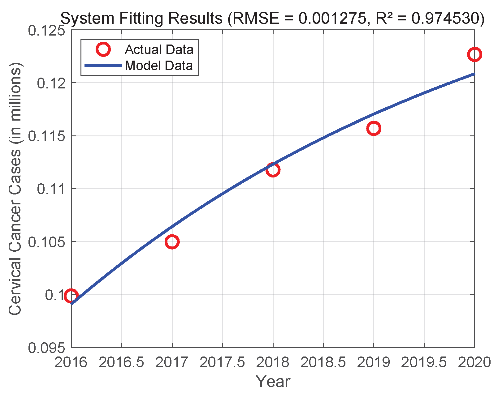
In order to verify the effectiveness and usefulness of system (3), we used actual data from India from 2016 to 2020 for numerical simulations and parameter calibration [20]. Initial parameters were set based on [16], with values: $\alpha =0.2$, $\beta =0.0012$, $\delta =0.05714$, $\rho =0.108696$, and $\gamma =0.5$. Utilizing MATLAB R2023a and its built-in dde23 solver, the DDE system was numerically resolved. The system parameters were calibrated by performing constrained nonlinear optimization using sequential quadratic programming within optimized parameter values. Figure 2 displays the final fitting results. The root mean square error (RMSE) of the fit is close to zero, indicating that System (3) and the actual data have excellent agreement. This suggests that System (3) has a high degree of practicality and predictive power, which may be used to predict the epidemiological dynamics of the disease in the Indian female population.

Therefore, we will use the calibrated parameter values $\mu =0.0138696$, $\mathsf{\Pi }=9.102635$, $\alpha =0.199998$, $\beta =0.001100$, $\delta =0.05700$, $\rho =0.118855$, and $\gamma =0.473409$ throughout the ensuing simulation process.

6.1. Sensitivity Analysis

The sensitivity of the basic reproduction number, $R_0$, to the system parameters is examined in this subsection using forward sensitivity analysis. We determine whether model parameters have a significant impact on $R_0$ by quantifying the relative influence of parameters on the value of $R_0$ by the calculation of sensitivity indices. After that, these parameters can be utilized to enhance intervention tactics.

Let $R_0$ be a differentiable function that depends on the parameter k, and let ${\mathsf{\Psi }}_k^{R_0}$ denote the Forward Normalized Sensitivity Index, which is defined by

$${\mathsf{\Psi }}_k^{R_0}={\displaystyle \frac{\partial R_0}{\partial k}}\times {\displaystyle \frac{k}{R_0}}.$$

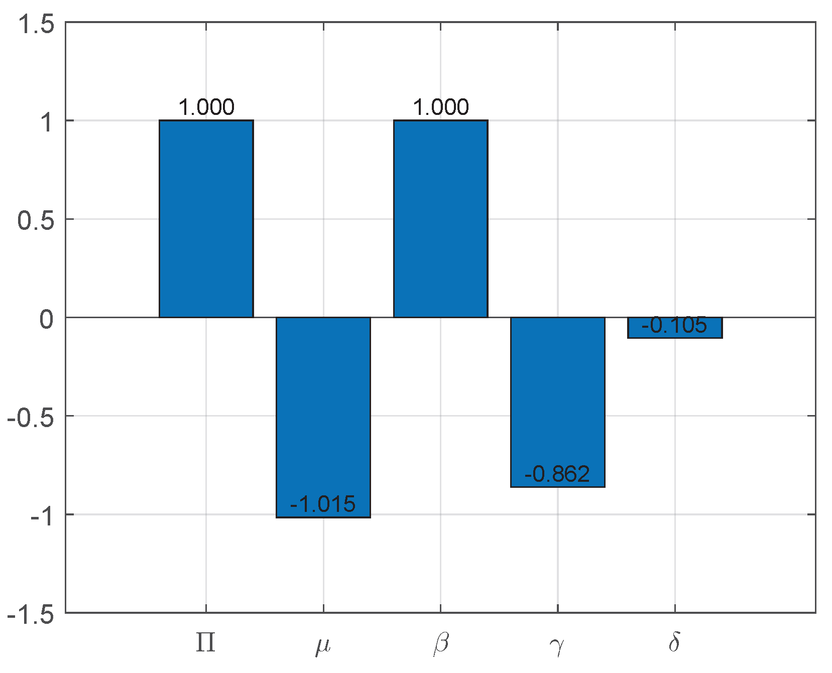
From the expression for ${\mathsf{\Psi }}_k^{R_0}$, we can obtain the sensitivity index of $R_0$, as shown in Figure 3:

Figure 3 shows the sensitivity indices for each parameter in detail. As can be observed, every parameter has a significant impact, with the exception of $\delta$. This indicates that a 10% drop in $\beta$ or $\mathsf{\Pi }$ causes a 10% drop in $R_0$ equivalently. Similarly, a 10% rise in $\gamma$ and $\delta$ causes the fundamental reproduction number $R_0$ to decrease by about 8.6% and 1%, respectively.

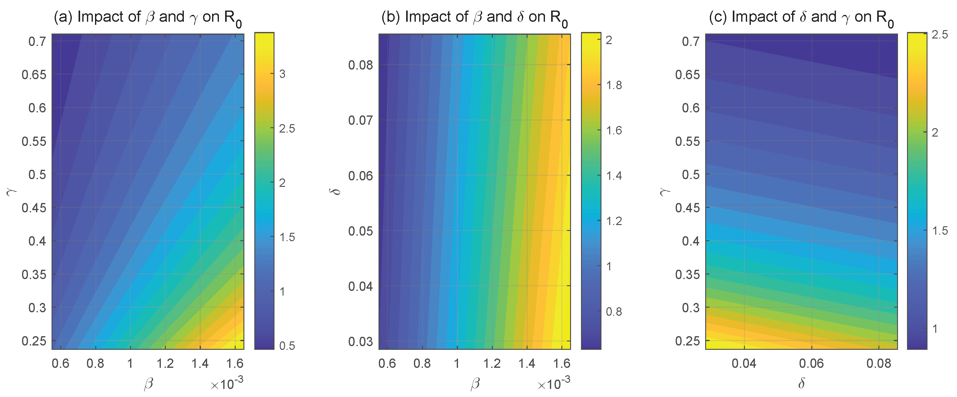
The sensitivity of $R_0$ to important system parameters is seen in Figure 4. The link between $R_0$ and HPV transmission rate $\beta$ and recovery rate $\gamma$ is seen in Figure 4a. It is evident that raising $\beta$ or lowering $\gamma$ causes $R_0$ to rise, while decreasing $\beta$ or raising $\gamma$ causes $R_0$ to fall. The effect of transmission rate $\beta$ and HPV with CC progression rate $\delta$ on $R_0$ is depicted in Figure 4b. Raising $\beta$ and lowering $\delta$ raise $R_0$, with $\beta$ having a notably stronger effect than $\delta$ to $R_0$. The fluctuation in $R_0$ with regard to progression rate $\delta$ and recovery rate $\gamma$ is seen in Figure 4c. $R_0$ decreases when $\delta$ and $\gamma$ are simultaneously raised, and it increases when they are simultaneously decreased. These results highlight the close relationship between $R_0$ and the two key system parameters, $\beta$ and $\gamma$. In order to lower the HPV transmission rate, $\beta$, it is advised to encourage safe sexual practices including using condoms and maintaining monogamy. Furthermore, the recovery rate, $\gamma$, can be effectively increased by enhanced individual immunity.

6.2. Numerical Simulations of the DDE System

In this subsection, the stability and Hopf bifurcation behavior are demonstrated using numerical simulation, based on the theoretical analysis of System (3). The stability of the system at the equilibrium point $E_1$ and the existence of the Hopf bifurcation are shown under various delay conditions by varying the time delay values ${\tau }_1$ and ${\tau }_2$. By the calibrated parameter values, we compute $R_0=1.326400>1$, the unique endemic equilibrium point of System (3) is $E_1=(494.79872727,22.05333046,9.47103880,48.81639443)$.

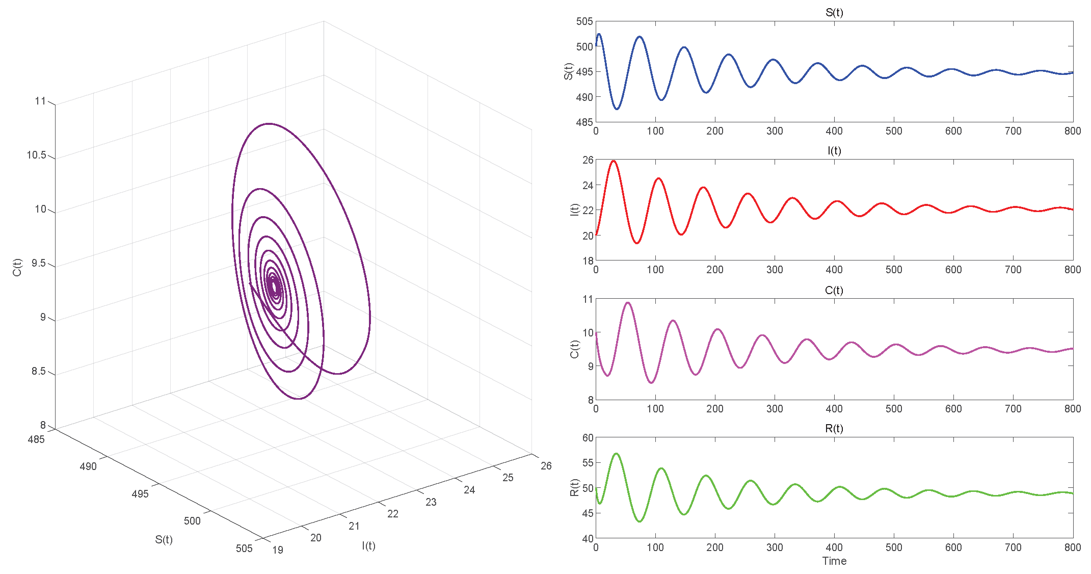
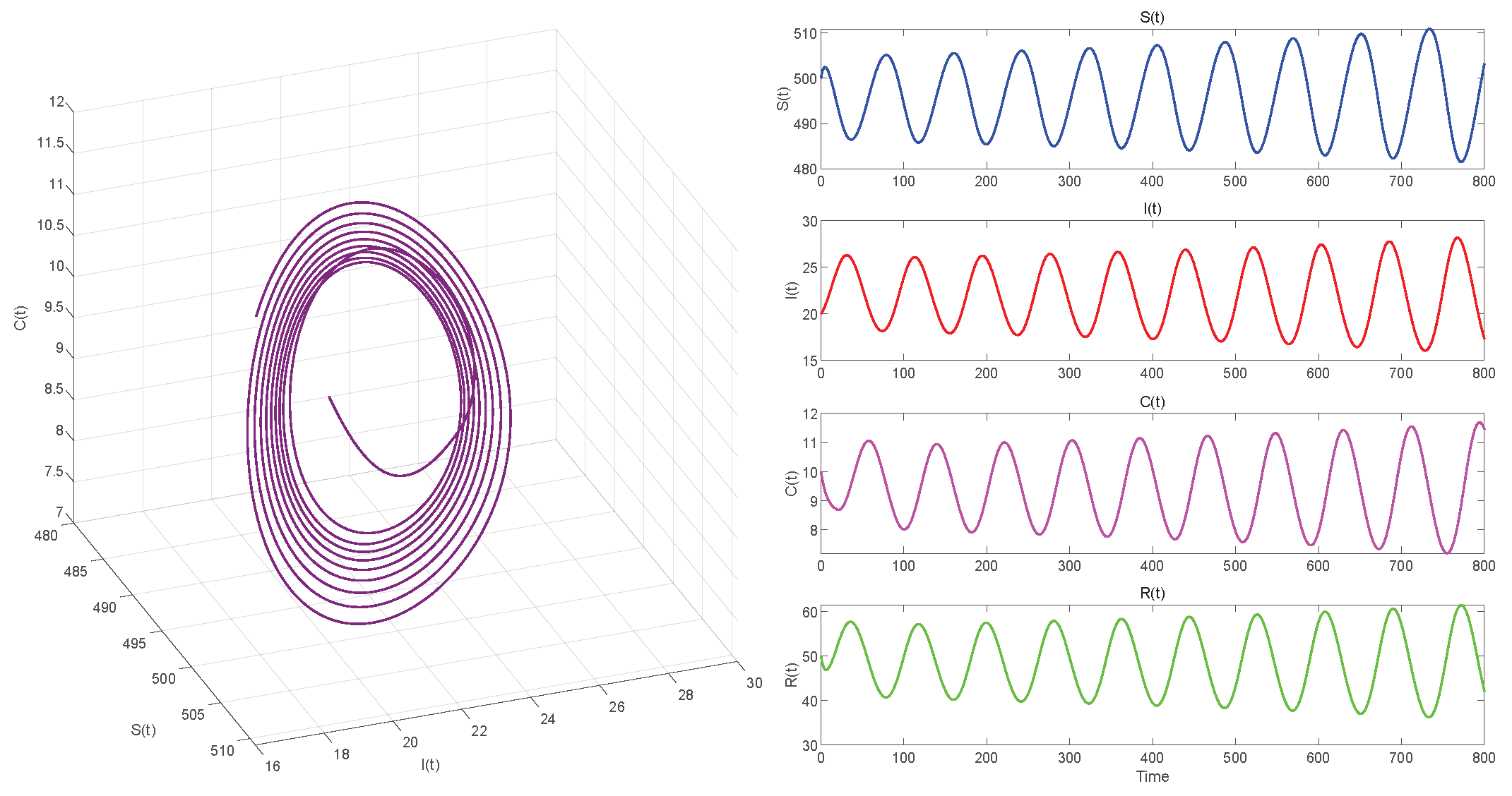
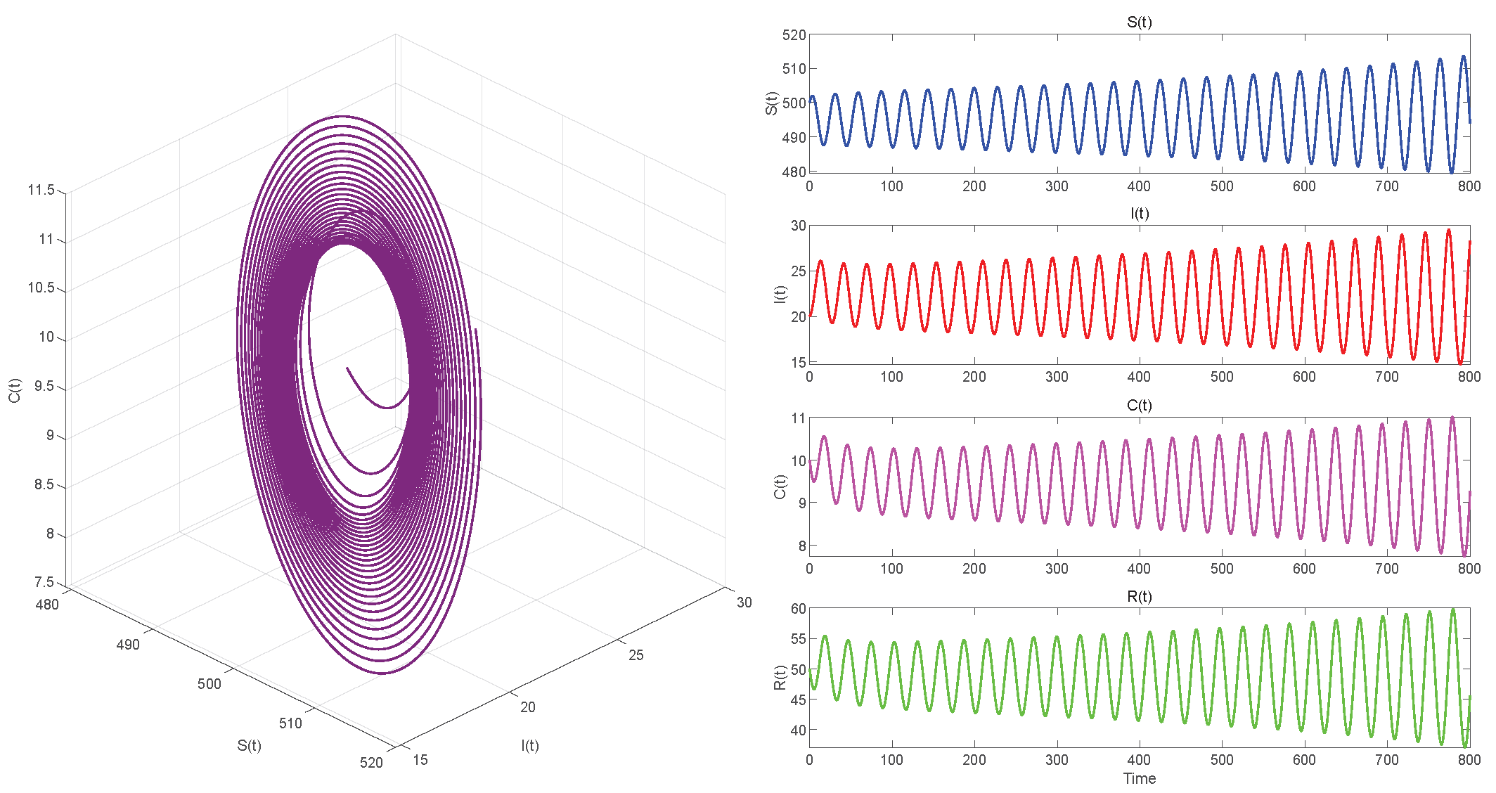
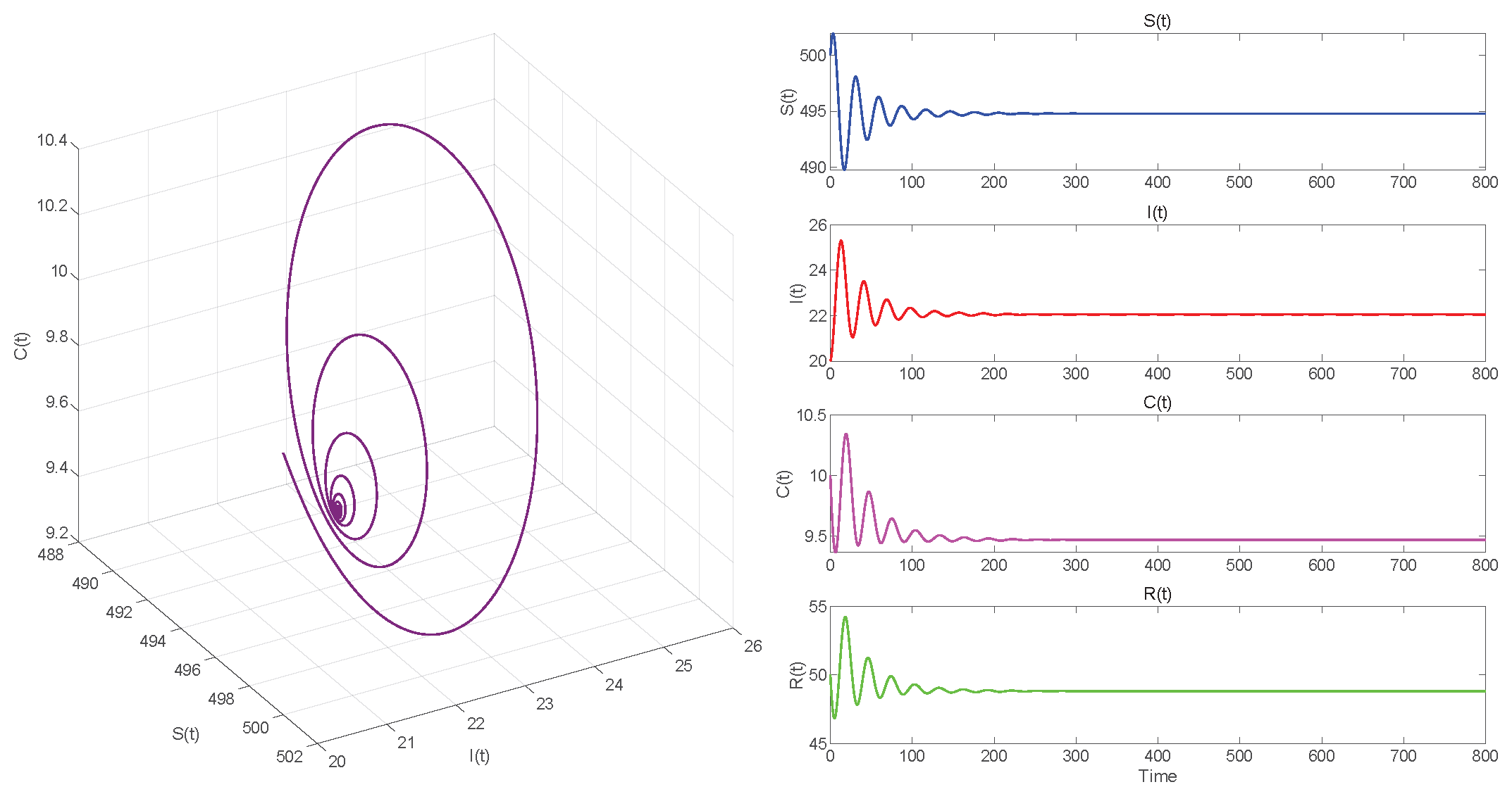
In Case 1, when ${\tau }_2=0$, we choose initial values $(500,20,10,50)$ close to the equilibrium point $E_1$. Using MATLAB R2023a with the dde23 solver to compute ${\omega }_{10}=0.06133514,{\tau }_{10}=19.0845$. If ${\tau }_1=17.2465<{\tau }_{10}$, the equilibrium point $E_1$ of the system is locally asymptotically stable, as seen in Figure 5. In Figure 6, we observe that the system has become unstable if ${\tau }_1=19.724>{\tau }_{10}$.

In Case 2, given ${\tau }_1=0$, we have ${\omega }_{20}=0.22960836,{\tau }_{20}=1.7656$. When ${\tau }_2=1.7273<{\tau }_{20}$, according to Figure 7, equilibrium point $E_1$ of System (3) is locally asymptotically stable. In Figure 8, one can see that the system has become unstable when ${\tau }_2=1.78>{\tau }_{20}$.

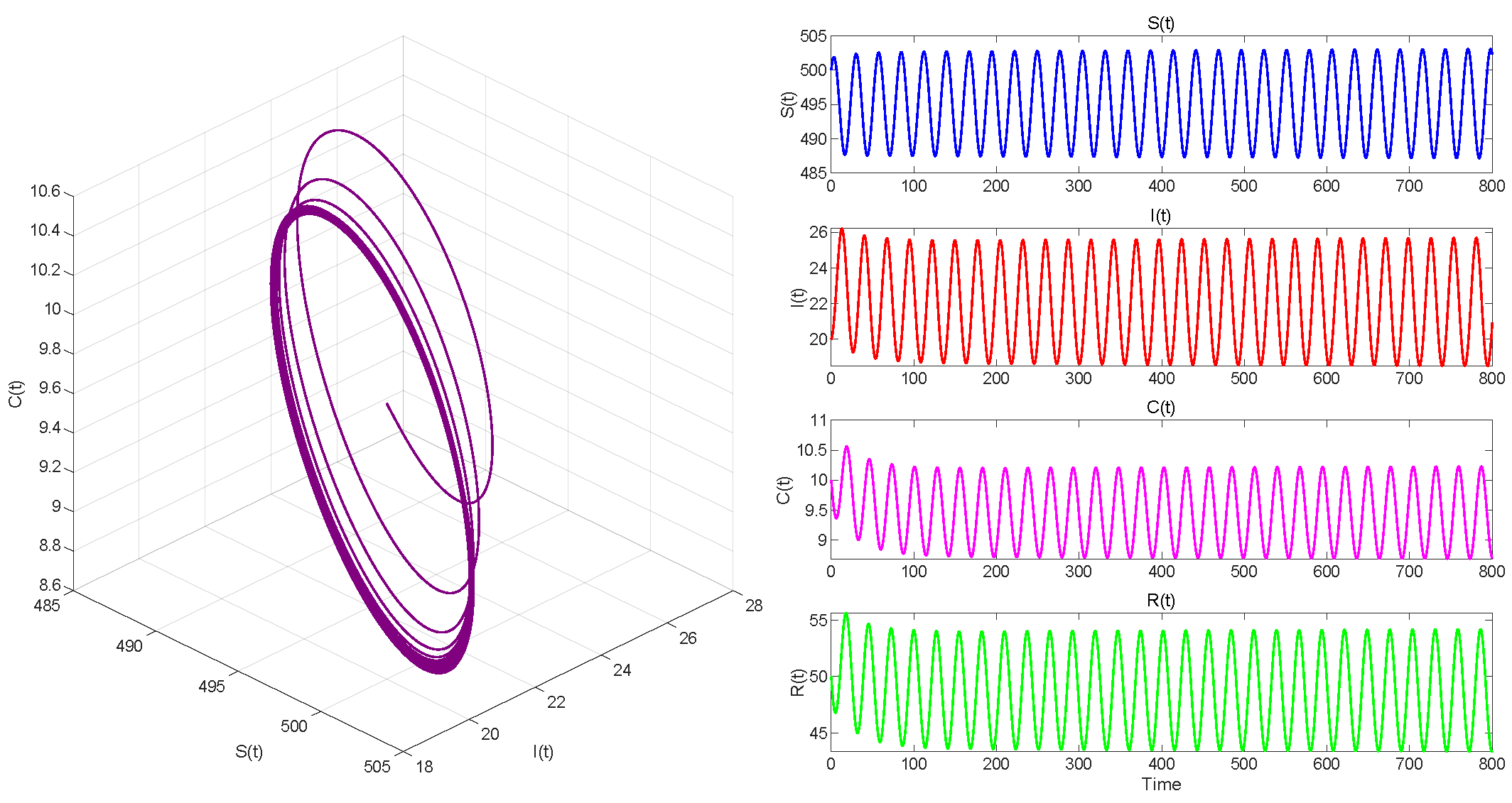
In Case 3, we take $(500,20,10,50)$. Then ${\omega }_{30}=0.23345663,{\tau }^{*}=1.5965$. When ${\tau }_1={\tau }_2=\tau =1.4712<{\tau }^{*}$, equilibrium point $E_1$ of System (3) is locally asymptotically stable in Figure 9. The Hopf bifurcation that occurs in System (3) when ${\tau }_1={\tau }_2=\tau =1.6017>{\tau }^{*}=1.5965$ is shown in Figure 10.

Figure 5, Figure 7 and Figure 9, respectively, illustrate the cases where ${\tau }_2=0$ with ${\tau }_1=17.2465<{\tau }_{10}$, ${\tau }_1=0$ with ${\tau }_2=1.7273<{\tau }_{20}$, and ${\tau }_1={\tau }_2=\tau =1.4712<{\tau }^{*}$. The phase space trajectory shows an inward spiral behavior towards the endemic equilibrium point $E_1$, as seen in the left panel. This contraction phenomenon suggests that minor perturbations would progressively decrease over time, stabilizing the system dynamics. The right panel shows the time evolution of each variable, which initially shows notable oscillations before stabilizing over time.

Figure 6, Figure 8 and Figure 10 demonstrate the cases where ${\tau }_2=0$ with ${\tau }_1=19.724>{\tau }_{10}$, ${\tau }_1=0$ with ${\tau }_2=1.78>{\tau }_{20}$, and ${\tau }_1={\tau }_2=\tau =1.6017>{\tau }^{*}$, respectively. The first two figures illustrate the Hopf bifurcation generated by the system under the action of time delay, showing instability as time progresses. The divergent state of the images can be clearly observed through the phase diagrams. The last figure depicts the critical transition. This continuous oscillation indicates a qualitative change from stability to sustained periodic behavior, revealing the appearance of a periodic solution through a Hopf bifurcation.

According to numerical simulation data, ${\tau }_1$ and ${\tau }_2$ are important bifurcation parameters that offer a mechanistic explanation of the instability caused by temporal delays in epidemic models.

6.3. Comparison with the ODE System and Discussion

To emphasize the crucial impact of the time-delay term on system dynamics, we conduct numerical simulations comparing the ordinary differential equation (OED) system (2) developed by Rajan et al. [16] (it can be obtained by setting the delays ${\tau }_1={\tau }_2=0$ in System (3)) to the DDE system (3) investigated in this study. We simultaneously account for the delay parameters ${\tau }_1$ and $\tau 2$ and use identical parameter values, employing ode45 and dde23 to solve systems (2) and (3), respectively.

By comparing Figure 11 and Figure 12, we can see that the ODE system quickly converges to a stable equilibrium point when a minor time delay ($\tau =1.4712<{\tau }^{*}$) is added. On the other hand, the convergence process of the DDE system shows a pronounced delayed response, even if it eventually stabilizes at the same equilibrium point. This illustrates how the transient behavior of the system can be greatly affected by even a small time delay, a feature that the ODE system is unable to account for. The system experiences a qualitative shift in behavior as the delays ${\tau }_1$ and ${\tau }_2$ rise above the critical threshold ($\tau =1.6017>{\tau }^{*}$). The time series shows that the DDE system no longer approaches equilibrium but instead displays steady and long-lasting periodic oscillations, as seen in Figure 12. However, ODE systems will still tend toward stability. The closed limit cycle in the phase diagram of Figure 11 definitively confirms the occurrence of a Hopf bifurcation. This suggests that the disease will exhibit periodic outbreaks rather than a sustained, stable presence. Indeed, continually increasing the time delay can lead to system divergence, implying a continuous increase in the number of infections that may result in an uncontrolled disease state. The preceding comparative analysis clearly demonstrates that neglecting the time delay will lead to an inaccurate assessment of the stability of the system and a complete inability to predict the risk of oscillatory instability as parameters change. Consequently, by developing a DDE system and analyzing its bifurcation behavior, we can successfully uncover these previously hidden, key dynamic characteristics, providing a more precise theoretical foundation for the analysis and control of the system.

7. Conclusions

In order to examine the dynamic interactions between HPV infection and CC, this research proposes a system of delay differential equations (DDEs) that incorporates dual delays. The study mainly looks at equilibrium point stability and existence, concentrating on two important delay parameters: the immune response delay (${\tau }_2$) and the cancerous delay (${\tau }_1$):

(i) 

The cancerous delay is the amount of time that passes between the start of a persistent infection with high-risk HPV strains and the final development of invasive cancer, which usually lasts 10–20 years or longer.

(ii) 

The immune response delay is the time required from pathogen invasion to the immune system effectively eliminating the pathogen and initiating the recovery process. In clinical terms, this refers to the window of time between infection and the virus or lesions being effectively removed by cellular immunity, usually between six months and two years.

Our theoretical analysis indicates that reducing ${\tau }_2$ and lengthening ${\tau }_1$ favor infection clearance. In contrast, prolonging ${\tau }_2$ and shortening ${\tau }_1$ greatly increase the probability of developing cancer. The combined action of ${\tau }_1$ and ${\tau }_2$ is noteworthy because it causes ${\tau }_1$ to destabilize the system earlier than in scenarios with a single delay (${\tau }_1$).

Our theoretical analysis was confirmed by the numerical simulations, which showed that the simulated values for ${\tau }_1$ and ${\tau }_2$ both fell within the boundaries of the theoretical analysis. Furthermore, by comparison, the DDE system and the ODE system showed that the DDE system had a greater variety of dynamic behaviors. These findings suggest that taking into account dual delays offers a more realistic framework for researching the complex dynamics of HPV infection.

Additionally, we examined the dynamic characteristics of Hopf bifurcations in the DDE system close to the equilibrium point, which showed that these delays may have an impact on the formation of periodic solutions. According to sensitivity analysis, the disease can be effectively managed by decreasing the transmission rate ($\beta$) and improving the recovery rate ($\gamma$), which suggests that condom use, monogamy, and improved immunity can help lower the incidence.

Although this study provides new understandings of the intricate relationships between HPV infection and the development of cancer, there are still issues that need to be addressed in subsequent studies. For example, male and female patients exhibit markedly different clinical presentations and pathological processes of the disease, according to [21]. Thus, taking into account the impact of gender, more research is needed on HPV infectious disease and CC systems with immune response delay and cancerous delay. In our upcoming work, these problems deserve more thought and resolution.

References

1. World Health Organization. Human Papillomavirus and Cancer. 2024. Available online: https://www.who.int/zh/news-room/fact-sheets/detail/human-papilloma-virus-and-cancer (accessed on 11 April 2025).
2. World Health Organization. Cervical Cancer. 2024. Available online: https://www.who.int/zh/news-room/fact-sheets/detail/cervical-cancer (accessed on 11 April 2025).
3. Tewari, K.S. Cervical cancer. N. Engl. J. Med. 2025, 392, 56–71. [Google Scholar] [CrossRef] [PubMed]
4. Snijders, P.J.; Steenbergen, R.D.; Heideman, D.A.; Meijer, C.J. HPV-mediated cervical carcinogenesis: Concepts and clinical implications. J. Pathol. 2005, 208, 152–164. [Google Scholar] [CrossRef] [PubMed]
5. Zhang, K.; Ji, Y.; Pan, Q.; Wei, Y.; Ye, Y.; Liu, H. Sensitivity analysis and optimal treatment control for a mathematical model of Human Papillomavirus infection. AIMS Math. 2020, 5, 2646–2670. [Google Scholar] [CrossRef]
6. Lee, S.L.; Tameru, A.M. A mathematical model of Human Papillomavirus (HPV) in the United States and its impact on cervical cancer. J. Cancer 2012, 3, 262–268. [Google Scholar] [CrossRef] [PubMed]
7. Obeng-Denteh, W.; Afrifa, R.T.; Barnes, B.; Addo, K.M. Modeling the epidemiology of Human Papilloma Virus infection and Vaccination and its impact on Cervical Cancer in Ghana. J. Sci. Res. Rep. 2014, 3, 2501–2518. [Google Scholar] [CrossRef]
8. Berhe, H.W.; Alarydah, M. Computational modeling of human papillomavirus with impulsive vaccination. Nonlinear Dyn. 2021, 103, 925–946. [Google Scholar] [CrossRef] [PubMed]
9. Nwajeri, U.K.; Panle, A.B.; Omame, A.; Obi, M.C.; Onyenegecha, C.P. On the fractional order model for HPV and Syphilis using non–singular kernel. Results Phys. 2022, 37, 105463. [Google Scholar] [CrossRef]
10. Abdeljawad, T.; Khan, N.; Abdalla, B.; Al-Jasern, A.; Alqudah, M.; Shah, K. A mathematical analysis of human papilloma virus (HPV) disease with new perspectives of fractional calculus. Alex. Eng. J. 2025, 125, 575–599. [Google Scholar] [CrossRef]
11. Gravitt, P.E. The known unknowns of HPV natural history. J. Clin. Investig. 2011, 121, 4593–4599. [Google Scholar] [CrossRef] [PubMed]
12. Crow, J.M. HPV: The global burden. Nature 2012, 488, S2–S3. [Google Scholar] [CrossRef] [PubMed]
13. Akimenko, V.V.; Adi-Kusumo, F. Age-structured delayed SIPCV epidemic model of HPV and cervical cancer cells dynamics I. Numerical method. Biomath 2021, 10, 2110027. [Google Scholar] [CrossRef]
14. Goel, A.N.; Frangos, M.; Raghavan, G.; Sangar, S.; Lazaro, S.; Wang, M.B.; Long, J.L.; St. John, M.A. Survival impact of treatment delays in surgically managed oropharyngeal cancer and the role of human papillomavirus status. Head Neck 2019, 41, 1756–1769. [Google Scholar] [CrossRef] [PubMed]
15. Vasudev, M.; Martin, E.; Frank, M.I.; Meller, L.L.T.; Haidar, Y.M. Treatment delay and HPV status on OPSCC with upfront surgery: Analysis of National Cancer Database. Otolaryngol.–Head Neck Surg. 2024, 171, 124–137. [Google Scholar] [CrossRef] [PubMed]
16. Rajan, P.K.; Kuppusamy, M.; Egbelowo, O.F. A mathematical model for human papillomavirus and its impact on cervical cancer in India. J. Appl. Math. Comput. 2023, 69, 753–770. [Google Scholar] [CrossRef]
17. Ismail, H.; Shangerganesh, L.; Msmali, A.H.; Bourazza, S.; Meetei, M.Z. Hopf Bifurcation and Optimal Control in an Ebola Epidemic Model with Immunity Loss and Multiple Delays. Axioms 2025, 14, 313. [Google Scholar] [CrossRef]
18. Hassard, B.D.; Kazarinoff, N.D.; Wan, Y.H. Theory and Applications of Hopf Bifurcation; Cambridge University Press: Cambridge, UK, 1981; Available online: https://www.google.com.tw/books/edition/Theory_and_Applications_of_Hopf_Bifurcat/3wU4AAAAIAAJ?hl=zh-CN&gbpv=0 (accessed on 15 May 2018).
19. Meng, X.-Y.; Huo, H.-F.; Xiang, H. Hopf bifurcation in a three-species system with delays. J. Appl. Math. Comput. 2010, 35, 635–661. [Google Scholar] [CrossRef]
20. Global Cancer Observatory: Cancer Today, International Agency for Research on Cancer. 2020. Available online: https://gco.iarc.fr/today/home (accessed on 1 May 2025).
21. Al-Arydah, M. Two-sex logistic model for human papillomavirus and optimal vaccine. Int. J. Biomath. 2021, 14, 2150011. [Google Scholar] [CrossRef]
Figure 1. Compartmental system structure of HPV-C dynamics.
Axioms 14 00680 g001
Figure 2. Fitting of System (3) to real data of cervical cancer individuals in India from 2016 to 2020.
Axioms 14 00680 g002
Figure 3. Sensitivity indices of R 0 to parameters of System (3).
Axioms 14 00680 g003
Figure 4. System parameter effects on R 0 .
Axioms 14 00680 g004
Figure 5. τ 2 = 0 , τ 1 = 17.2465 < τ 10 = 19.0845 . Equilibrium E 1 of System (3) is locally asymptotically stable.
Axioms 14 00680 g005
Figure 6. τ 2 = 0 , τ 1 = 19.724 > τ 10 = 19.0845 . Equilibrium E 1 of System (3) is unstable.
Axioms 14 00680 g006
Figure 7. τ 1 = 0 , τ 2 = 1.7273 < τ 20 = 1.7656 . Endemic equilibrium E 1 of System (3) is locally asymptotically stable.
Axioms 14 00680 g007
Figure 8. τ 1 = 0 , τ 2 = 1.78 > τ 20 = 1.7656 . Equilibrium E 1 of System (3) is unstable.
Axioms 14 00680 g008
Figure 9. τ 1 = τ 2 = τ = 1.4712 < τ * . Equilibrium E 1 of System (3) is locally asymptotically stable.
Axioms 14 00680 g009
Figure 10. τ 1 = τ 2 = τ = 1.6017 > τ * = 1.5965 . Hopf bifurcation occurs.
Axioms 14 00680 g010
Figure 11. Comparison of the time evolution of the infective population ( S ( t ) , I ( t ) , C ( t ) , R ( t ) ). Left panel: τ 1 = τ 2 = τ = 1.4712 < τ * = 1.5965 . Both systems stabilize at an endemic equilibrium point E 1 , though the DDE response shows slight overshoot. Middle panel: τ 1 = τ 2 = τ = 1.6017 > τ * . The ODE system stabilizes, while the DDE system exhibits sustained oscillations. Right panel: τ τ * . The ODE system stabilizes, whereas the DDE solution grows unbounded, indicating system instability.
Axioms 14 00680 g011
Figure 12. Comparison of Phase Portraits between ODE and DDE systems under Different Time Delays. Left panel: ODE and DDE systems for τ 1 = τ 2 = τ = 1.4712 < τ * = 1.5965 . Both systems converge to a stable equilibrium point. Middle panel: For τ 1 = τ 2 = τ = 1.6017 > τ * . The ODE system remains stable, while the DDE system undergoes a Hopf bifurcation, forming a stable limit cycle (periodic oscillation). Right panel: For τ τ * . The ODE system remains stable, whereas the DDE system becomes unstable and diverges.
Axioms 14 00680 g012