Bayesian Inference for Copula-Linked Bivariate Generalized Exponential Distributions: A Comparative Approach

Abstract

This paper addresses the limitations of existing bivariate generalized exponential (GE) distributions for modeling lifetime data, which often exhibit rigid dependence structures or non-GE marginals. To overcome these limitations, we introduce four new bivariate GE distributions based on the Farlie–Gumbel–Morgenstern, Gumbel–Barnett, Clayton, and Frank copulas, which allow for more flexible modeling of various dependence structures. We employ a Bayesian framework with Markov Chain Monte Carlo (MCMC) methods for parameter estimation. A simulation study is conducted to evaluate the performance of the proposed models, which are then applied to a real-world dataset of electrical treeing failures. The results from the data application demonstrate that the copula-based models, particularly the one derived from the Frank copula, provide a superior fit compared to existing bivariate GE models. This work provides a flexible and robust framework for modeling dependent lifetime data.

1. Introduction

The univariate generalized exponential (GE) is a versatile distribution introduced by [1] with several interesting properties that can be used quite effectively to analyze lifetime data. It is a good alternative to the usual lifetime distributions as Weibull and Gamma distributions. Although several studies have been conducted on the GE distribution, research on the bivariate GE distributions remains limited.

While the foundational work on bivariate copulas remains essential, the field has seen significant advances in recent years. Contemporary research has largely focused on developing highly flexible models for high-dimensional data, particularly using vine copulas or pair-copula constructions (e.g., [2]). Bayesian non-parametric copulas using infinite partitions of unity have been introduced to capture both central and tail dependence through stick-breaking priors [3]. Ref. [4] developed Dirichlet process mixtures of Archimedean copulas that allow arbitrary dimension and complex dependence patterns. Ref. [5] proposed approximate Bayesian conditional copulas to incorporate covariate effects into the copula function without fixed parametric forms. Furthermore, ref. [6] integrated vine copula constructions with Bayesian non-parametric priors to flexibly model high-dimensional conditional dependence structures. Furthermore, there is a growing body of literature on dynamic copula models that allow the dependence structure to evolve over time [7]. The current work contributes to a parallel stream of research that continues to develop novel bivariate distributions with specific, practical marginals, such as the generalized exponential, to provide flexible and interpretable models for lifetime and reliability data.

In recent years, some representations of bivariate GE distribution have been proposed. Refs. [8,9] have introduced a bivariate distribution using the GE and exponential distribution. However, the marginal distributions do not have known forms. Ref. [10] introduced a singular bivariate generalized exponential distribution (BVGE), whose marginals are GE distributions. The authors present several probabilistics properties, including the maximum likelihood estimation (MLE). Ref. [11] used the Bayesian approach to estimate the parameters of BVGE. Ref. [12] considered the Bayesian inference of the unknown parameters of this distribution obtained by using different prior distributions as uniform, gamma distributions and the objective Jeffreys prior. Ref. [13] also derived an absolute continuous BVGE distribution by using transformation from bivariate exchangeable distribution. The marginals of the proposed BVGE are also GE.

Ref. [14] introduced an absolutely continuous bivariate generalized exponential distribution by using the method of [15]. This new distribution was obtained from the bivariate generalized exponential distribution (BVGE) model by removing the singular part. In this case, the marginal distributions are not a generalized exponential.

Besides generalizations, copula functions have become a popular tool for modeling the dependence between multivariate data; see, for example, [16,17]. The copula approach allows the construction of unknown bivariate distributions based on known marginals. Ref. [18] wrote a compendium on copulas, where they presented an updated review on this important subject.

Copula functions have been effectively applied to model the dependence structure of the generalized exponential (GE) distribution, offering flexibility in capturing complex multivariate relationships. Refs. [19,20] further contributed to this field by proposing novel methodologies for incorporating copula functions into the modeling of dependent lifetimes with GE marginals, such as the Farlie–Gumbel–Morgensten and Clayton copulas. Their contributions include both classical and Bayesian inference procedures, demonstrating the flexibility and practical relevance of copula-based GE models in survival analysis and reliability studies. The integration of copulas with the GE distribution, as explored by these authors, provides a robust framework for analyzing multivariate non-normal data.

The existing bivariate GE distributions face limitations: rigid dependence structures, singular components, or non-GE marginals, restricting their utility for real-world lifetime data with complex dependencies. To address this, we present four different bivariate generalized exponential distributions obtained by using the Farlie–Gumbel–Morgenstern, Gumbel–Barnett, Clayton, and Frank copulas compounded with GE marginal distributions.

Although copulas are able to capture several different dependence structures of two or more random variables, an incorrect choice of copula may result in a poor fit to the data. To select a more appropriate copula, this paper considers three levels of dependence: weak, moderate, and strong, for each of the BVGE distributions generated. Also, we investigate the performance of the resulting BVGE distributions through a simulation study. We assess fidelity to data generated from bivariate Weibull distributions, a neutral benchmark that avoids favoring any GE-based model.

Given the complexity of the proposed bivariate generalized exponential distributions derived using the Farlie–Gumbel–Morgenstern, Gumbel–Barnett, Clayton, and Frank copulas, obtaining the parameter estimates through traditional analytical methods is not straightforward. The likelihood functions for these models can be complex, making direct maximization challenging. Therefore, a Bayesian approach under non-informative priors and using Markov Chain Monte Carlo (MCMC) methods provides a robust and flexible alternative for parameter estimation. This computational approach allows us to simulate samples from the posterior distributions of the model parameters, providing not only point estimates but also credible intervals that capture the uncertainty in the obtained estimates. To implement this Bayesian analysis, we utilized the OpenBUGS 3.2. [21] software, which is a powerful and widely used tool for performing MCMC simulations.

Finally, a real-life data (electrical treeing failures) set was used in order to illustrate the usefulness of the proposed distributions.

The paper is organized as follows. Section 2 introduces copula functions, focusing on the Farlie–Gumbel–Morgenstern, Gumbel–Barnett, Clayton, and Frank copulas. Section 3 presents the derivation of the bivariate generalized exponential distribution using copulas. In Section 4, three bivariate models are presented: the BGE, the BVGE, and the the generalized bivariate exponential distribution Block–Basu (BBBGE) distributions. Section 5 details the Bayesian analysis, including prior distributions for the model parameters. Section 6 evaluates the performance of the bivariate models through simulations to determine which best captures data characteristics. Section 7 applies the models to a real-world survival time dataset in electrical engineering. Finally, Section 8 summarizes the findings and conclusions of the study.

2. Copula Function

Copula functions link marginal distributions to form a joint distribution. For specified univariate marginal distribution functions $F(t_1,t_2,\dots ,t_m)$, the function $C(F_1\left(t_1\right)$, $F_2\left(t_2\right)$, …, $F_m\left(t_m\right))$ is defined using a copula function C, resulting in a multivariate distribution defined via the copula function. It is important to note that any multivariate distribution function $F(.)$ can be written in the form of a copula function [22]; that is, if $F(t_1,t_2,\dots ,t_m)$ is a joint multivariate distribution function with univariate marginal distribution functions $F_1\left(t_1\right),F_2\left(t_2\right),\dots ,F_m\left(t_m\right)$, there exists a copula function $C(u_1,u_2,\dots ,u_m)$ such that

$$F(t_1,t_2,\dots ,t_m)=C\left(F_1\left(t_1\right),F_2\left(t_2\right),\dots ,F_m\left(t_m\right)\right).$$

(1)

If $f(t_1,t_2,\dots ,f_m)$ and $f_1\left(t_1\right),f_2\left(t_2\right),\dots ,f_m\left(t_m\right)$ denote the joint density and marginal densities of $T_1,T_2,\dots ,T_m$, respectively, with distribution function $F(t_1,t_2,\dots ,t_m)$, then the joint density can be written in terms of the copula density and the marginal densities as

$$f(t_1,t_2,\dots ,t_m)=\left(\prod _{i=1}^n{f}_i\left(t_i\right)\right)c\left(F_1\left(t_1\right),F_2\left(t_2\right),\dots ,F_m\left(t_m\right)\right),$$

(2)

where $c(u_1,u_2,\dots ,u_m)={\displaystyle \frac{{\partial }^{m}C(u_1,u_2,\dots ,u_m)}{\partial u_1\partial u_2\dots \partial u_m}}$ is the copula density of C.

Specifically, the dependence between $T_1$ and $T_2$ is equivalent to specifying dependence between $U_1=F_1\left(t_1\right)$ and $U_2=F_2\left(t_2\right)$. Thus, the problem reduces to defining a bivariate distribution for two uniform variables; that is, a copula.

Different copula functions introduced in the literature could be used to obtain a bivariate distribution with GE marginals. The first model considered for the study of the dependence structure for two variables is based on the Farlie–Gumbel–Morgenstern (FGM) copula; see, for example, [23].

In this section, we review some copula-based bivariate models that shall be employed to obtain bivariate generalized exponential distributions.

2.1. Farlie–Gumbel–Morgenstern Copula

The first model considered for the study of dependence structure for two variables is based on the Farlie–Gumbel–Morgenstern (FGM) copula defined by

$$C_I(u_1,u_2)=u_1{u}_2\left(1+\theta (1-u_1)(1-u_2)\right),$$

(3)

where $u_1=F_1\left(t_1\right)$ and $u_2=F_2\left(t_2\right)$ and $-1<\theta <1$. Observe that $\theta$ measures the dependence between two marginals; that is, if $\theta =0$, we have independent random variables. This copula is appropriated to model weak dependence structures.

The association parameter $\theta$ can take different values depending on the copula, whereas measures of association, such as Pearson’s correlation coefficient that is usually bounded. The parameter $\theta$ is related to the well-known association coefficients Kendall’s Tau $\left(\tau \right)$ and Spearman’s Rho $\left(\rho \right)$ by the equations

$$\begin{array}{c}\hfill \tau =4\int \int C(u_1,u_2)dC(u_1,u_2)-1={\displaystyle \frac{2\theta }{9}},\\ \hfill \rho =12\int \int C(u_1,u_2)dC(u_1,u_2)-3={\displaystyle \frac{\theta }{3}}.\end{array}$$

(4)

The correlation coefficient clearly ranges from $-{\displaystyle \frac{1}{3}}$ to ${\displaystyle \frac{1}{3}}$.

Now, for the FGM copula $C_I$ given in the Equation (3), the corresponding copula density $c_I$ is

$$c_I(u_1,u_2)=1+\theta (1-2u_1)(1-2u_2).$$

(5)

Let $(T_1,T_2)$ denote the paired random variables with $(F_1\left(t_1\right),F_2\left(t_2\right))$, $(f_1\left(t_1\right),f_2\left(t_2\right))$ denoting the corresponding marginal cumulative and density functions, respectively, then the joint cumulative distribution function and density for the random variables $T_1$ and $T_2$ become

$$F_I(t_1,t_2)=C_I\left(F_1\left(t_1\right),F_2\left(t_2\right)\right)=F_1\left(t_1\right)F_2\left(t_2\right)[1+\theta (1-F_1\left(t_1\right))(1-F_2\left(t_2\right))]$$

(6)

and

$$f_I(t_1,t_2)=f_1\left(t_1\right)f_2\left(t_2\right)[1+\theta (1-2F_1\left(t_1\right))(1-2F_2\left(t_2\right))],$$

(7)

respectively. The bivariate survival function $S_I(t_1,t_2)$ of the FGM copula is given by

$$S_I(t_1,t_2)=S_1\left(t_1\right)+S_2\left(t_2\right)-1+\left(1+\theta F_1\left(t_1\right)F_2\left(t_2\right)\right),$$

(8)

where $S_1\left(t_1\right)$ and $S_2\left(t_2\right)$ are the marginal survival functions of $T_1$ and $T_2$, respectively.

2.2. Gumbel–Barnett Copula

The second copula function to be considered for the study of dependence structure for two variables is the Gumbel–Barnett copula [24], defined by

$$C_{II}(u_1,u_2)=u_1+u_2-1+(1-u_1)(1-u_2)exp\{-\varphi ln(1-u_1)ln(1-u_2)\},$$

(9)

where $\varphi$ is the dependence parameter restricted to the interval $(0,1)$.

Ref. [25] showed that the conditional copula of Gumbel–Barnett copula is also a Gumbel–Barnett copula. He also deduced its properties and its importance in applications.

The density of this copula is given by

$$\begin{array}{ccc}\hfill c_{II}(u_1,u_2)& =& \left\{-\varphi +[1-\varphi ln(1-u_1)][1-\varphi ln(1-u_2)\right\}\hfill \\ & \times & exp\{-\varphi ln(1-u_1)ln(1-u_2)\}.\hfill \end{array}$$

(10)

The corresponding Kendall’s Tau $\left(\tau \right)$ coefficient is given by

$$\tau =-e^{{\displaystyle \frac{2}{\varphi }}}{\int }_{{\displaystyle \frac{2}{\varphi }}}^{\infty }{\displaystyle \frac{e^{-x}}{x}}dx<0$$

(11)

and the Spearman’s Rho $\left(\rho \right)$ coefficient is given by

$$\rho =12{\int }_0^1{\displaystyle \frac{u}{2-\varphi lnu}}du-3.$$

(12)

Both integrals (11) and (12) can be obtained by numerical integration.

In this model, the joint cumulative distribution function for the random variables $X_1$ and $X_2$ is given by

$$\begin{array}{ccc}\hfill F_{II}(t_1,t_2)& =& F_1\left(t_1\right)+F_2\left(t_2\right)-1+[1-F_1\left(t_1\right)][1-F_2\left(t_2\right)]\hfill \\ & \times & exp\{-\varphi ln(1-F_1\left(t_1\right))ln(1-F_2\left(t_2\right))\}\hfill \end{array}$$

(13)

and the corresponding joint density function for $T_1$ and $T_2$ is given by

$$\begin{array}{ccc}\hfill f_{II}(t_1,t_2)& =& [-\varphi +(1-\varphi ln(1-F_1\left(t_1\right)))(1-\varphi ln(1-F_2\left(t_2\right)))]\hfill \\ & \times & exp\{-\varphi ln(1-F_1\left(t_1\right))ln(1-F_2\left(t_2\right))\}.\hfill \end{array}$$

(14)

The joint survival function for the lifetimes $T_1$ and $T_2$ can also be obtained as

$$S_{II}(t_1,t_2)=S_1\left(t_1\right)S_2\left(t_2\right)exp\{-\varphi ln{S}_1\left(t_1\right)ln{S}_2\left(t_2\right)\}.$$

(15)

2.3. Clayton Copula

A well-known copula is the Clayton copula introduced by [26]. The Clayton copula is an Archimedean asymmetric copula given by

$$C_{III}(u_1,u_2)={\left(u_1^{-\alpha }+u_2^{-\alpha }-1\right)}^{-{\displaystyle \frac{1}{\alpha }}},0<\alpha <\infty .$$

(16)

The density function $c_{III}(u_1,u_2)$ of copula (16) is given by

$$c_{III}(u_1,u_2)=(\alpha +1){\left(u_1{u}_2\right)}^{-\alpha +1}{\left(u_1^{-\alpha }+u_2^{-\alpha }-1\right)}^{-\left({\displaystyle \frac{1}{\alpha }}+2\right)}.$$

(17)

The Clayton copula has been used to study correlated risks because it exhibits strong left-tail dependence and relatively weak right-tail dependence.

Note that it does not allow negative dependence between the marginal distributions. Moreover, when $\alpha =0$, we have independence, while $\alpha ⟶\infty$ implies perfect positive dependence.

The relationship between the parameter $\alpha$ and the Kendall’s Tau $\left(\tau \right)$ measure is given by

$$\tau ={\displaystyle \frac{\alpha }{\alpha +2}}.$$

(18)

The Spearman’s Rho $\left(\rho \right)$ measure for this copula is very complicated.

The joint cumulative function of the Clayton copula (16) is given by

$$F_{III}(t_1,t_2)=C_{III}\left(F_1\left(t_1\right),F_2\left(t_2\right)\right)={\left(F_1{\left(t_1\right)}^{-\alpha }+F_2{\left(t_2\right)}^{-\alpha }-1\right)}^{-{\displaystyle \frac{1}{\alpha }}}$$

(19)

and the corresponding joint density function for $T_1$ and $T_2$ is given by

$$f_{III}(t_1,t_2)=(\alpha +1)f_1\left(t_1\right)f_2\left(t_2\right){\left(F_1\left(t_1\right),F_2\left(t_2\right)\right)}^{-(\alpha +1)}{\left(F_1{\left(t_1\right)}^{-\alpha }+F_2{\left(t_2\right)}^{-\alpha }-1\right)}^{-({\displaystyle \frac{1}{\alpha }}+2)}.$$

(20)

The joint survival function based on the Clayton copula can be expressed as

$$S_{III}(t_1,t_2)=S_1\left(t_1\right)+S_2\left(t_2\right)-1+{\left(F_1{\left(t_1\right)}^{-\alpha }+F_2{\left(t_2\right)}^{-\alpha }-1\right)}^{-{\displaystyle \frac{1}{\alpha }}}.$$

(21)

2.4. Frank Copula

Another alternative copula is the Frank copula [27] that takes the form

$$C_{IV}(u_1,u_2)=-{\displaystyle \frac{1}{\phi }}ln\left(1+{\displaystyle \frac{(e^{-\phi u_1}-1)(e^{-\phi u_2}-1)}{e^{-\phi }-1}}\right),$$

(22)

with dependence parameter $\phi \ne 0$.

The density function $c_{IV}(u_1,u_2)$ of the copula (22) is given by

$$c_{IV}(u_1,u_2)={\displaystyle \frac{\phi (1-e^{-\phi })\left(1+e^{-\phi (u_1+u_2)}\right)}{{\left[\left(e^{-\phi u_1}-1\right)(e^{-\phi u_2}-1)+e^{-\phi }-1\right]}^2}}.$$

(23)

Unlike the Clayton and Gumbel-Barnett copulas, which are restricted to positive dependence, the Frank copula accommodates both positive and negative dependence. However, it is most appropriate for data that exhibit weak tail dependence.

The relationship between the Frank copula parameter $\phi$ and the coefficients Kendall’s Tau $\left(\tau \right)$, and Spearman’s Rho $\left(\rho \right)$ are given by the equations

$$\tau =1-{\displaystyle \frac{4}{\phi }}\left[1-D_1\left(\phi \right)\right]\mathrm{and}\rho =1-{\displaystyle \frac{12}{\phi }}\left[D_1\left(\phi \right)-D_2\left(\phi \right)\right],$$

(24)

respectively, where $D_k\left(x\right)={\displaystyle \frac{k}{x^k}}{\int }_0^x{\displaystyle \frac{t^k}{e^t-1}}dt$ is a Debye function of the k-th kind.

The joint cumulative function of the Frank copula (22) is given by

$$F_{IV}(t_1,t_2)=-{\displaystyle \frac{1}{\phi }}ln\left[1+{\displaystyle \frac{(e^{-\phi F_1\left(t_1\right)}-1)(e^{-\phi F_2\left(t_2\right)}-1)}{e^{-\phi }-1}}\right]$$

(25)

and the corresponding joint density function for $T_1$ and $T_2$ is given by

$$f_{IV}(t_1,t_2)={\displaystyle \frac{\phi (-e^{\phi }-1)f_1\left(t_1\right)f_2\left(t_2\right)exp\{-\phi \left[F_1\left(t_1\right)F_2\left(t_2\right)\right]\}}{{[e^{-\phi }-1+(e^{-\phi F_1\left(t_1\right)}-1)(e^{-\phi F_2\left(t_2\right)}-1)]}^2}}.$$

(26)

The joint survival function can be expressed as

$$S_{IV}(t_1,t_2)=S_1\left(t_1\right)+S_2\left(t_2\right)-1-{\displaystyle \frac{1}{\phi }}ln\left[1+{\displaystyle \frac{(e^{-\phi F_1\left(t_1\right)}-1)(e^{-\phi F_2\left(t_2\right)}-1)}{e^{-\phi }-1}}\right].$$

(27)

2.5. Copula Selection Criteria

To ensure that the comparison covers a broad spectrum of dependence structures, we select four classical copula families with distinct tail-dependence properties and overall dependence ranges, commonly found in lifetime data. The selected copulas, FGM, Gumbel–Barnett, Clayton, and Frank, each offer different properties:

• FGM copula. It models weak to moderate symmetric dependence ($\theta \in [-1,1]$; no tail dependence), ideal for scenarios where extreme-value dependence is negligible [16].
• Gumbel–Barnett copula. It captures negative and upper-tail dependence, making it suitable for modeling the simultaneous occurrence of large values (late failures), ($\varphi \in (0,1]$), rare in survival data but critical for robustness checks.
• Clayton copula. It has a strong lower-tail dependence (i.e., when both variables have low values, they are highly correlated for $\alpha >0$), suitable for joint early failures (e.g., system shocks).
• Frank copula. It is a flexible symmetric dependence ($\phi \in {\mathbb{R}}_{\ne 0}$), accommodating both positive/negative associations without tail dependence [28]. Its flexibility in the body of the distribution makes it a natural contrast to FGM.

Table 1. Properties of selected copulas and their suitability for GE marginals.

Copula	Dependence Range	Tail Dependence	Suitability for GE Marginals
FGM	$\theta \in (-1,1)$	None	Weak/moderate symmetric dependence
Gumbel–Barnett	$\varphi \in (0,1]$	Upper-tail	Negative dependence
Clayton	$\alpha >0$	Lower-tail	Early failure scenarios
Frank	$\phi \in {\mathbb{R}}_{\ne 0}$	None	Flexible symmetric dependence

compares their properties, and the coming simulation (Section 6) validates their complementary roles in capturing GE-based dependence.

By including both symmetric, tail-independent families (FGM and Frank) and asymmetric, tail-dependent families (Clayton and Gumbel–Barnett), the current study systematically evaluates model performance under weak versus strong dependence and lower- versus upper-tail behavior.

Furthermore, by comparing these four families, we can empirically determine which dependence structure is the most suitable for the dataset under consideration, providing a comprehensive analysis that is not limited to a single type of association.

3. Bivariate Generalized Exponential Distribution Derived from Copulas

In this section, we construct the bivariate generalized exponential distribution based on the four copulas stated in Section 2. We derive the bivariate joint survival functions.

Let us assume the marginal generalized exponential distributions $T_1\sim GE({\alpha }_1,{\lambda }_1)$ and $T_2\sim GE({\alpha }_2,{\lambda }_2)$ with distributions functions given by

$$F_1\left(t_1\right)={\left(1-e^{-{\lambda }_1{t}_1}\right)}^{{\alpha }_1}\mathrm{and}{F}_2\left(t_2\right)={\left(1-e^{-{\lambda }_2{t}_2}\right)}^{{\alpha }_2}$$

(28)

and respective marginal densities

$$f_1\left(t_1\right)={\alpha }_1{\lambda }_1{\left(1-e^{-{\lambda }_1{t}_1}\right)}^{{\alpha }_1-1}{e}^{{\lambda }_1{t}_1}\mathrm{and}{f}_2\left(t_2\right)={\alpha }_2{\lambda }_2{\left(1-e^{-{\lambda }_2{t}_2}\right)}^{{\alpha }_2-1}{e}^{{\lambda }_2{t}_2}.$$

(29)

Choosing the Farlie–Gumbel–Morgenstern copula yields the joint density function obtained from Equation (7) as

$$\begin{array}{ccc}\hfill f_I(t_1,t_2)& =& {\alpha }_1{\alpha }_2{\lambda }_1{\lambda }_2{e}^{-({\lambda }_1{t}_1+{\lambda }_2{t}_2)}{\left(1-e^{-{\lambda }_1{t}_1}\right)}^{{\alpha }_1-1}{\left(1-e^{-{\lambda }_2{t}_2}\right)}^{{\alpha }_2-1}\hfill \\ & \times & \left[1+\theta (1-2{(1-e^{-{\lambda }_1{t}_1})}^{{\alpha }_1})(1-2{(1-e^{-{\lambda }_2{t}_2})}^{{\alpha }_2})\right]\hfill \end{array}$$

(30)

and the corresponding joint survival function is given by

$$S_I(t_1,t_2)=\left(1-{(1-e^{-{\lambda }_1{t}_1})}^{{\alpha }_1}\right)\left(1-{(1-e^{-{\lambda }_2{t}_2})}^{{\alpha }_2}\right)\left[1+\theta {(1-e^{-{\lambda }_1{t}_1})}^{{\alpha }_1}{(1-e^{-{\lambda }_2{t}_2})}^{{\alpha }_2}\right].$$

(31)

Now, if we assume the Gumbel–Barnett copula with the generalized exponential marginals Equations (28) and (29), then the corresponding bivariate density and survival distributions are given by

$$\begin{array}{ccc}\hfill f_{II}(t_1,t_2)& =& {\alpha }_1{\alpha }_2{\lambda }_1{\lambda }_2{e}^{-({\lambda }_1{t}_1+{\lambda }_2{t}_2)}{(1-e^{-{\lambda }_1{t}_1})}^{{\alpha }_1-1}{(1-e^{-{\lambda }_2{t}_2})}^{{\alpha }_2-1}\hfill \\ & \times & \left[-\varphi +\left(1-\varphi ln\left(1-{(1-e^{-{\lambda }_1{t}_1})}^{{\alpha }_1}\right)\right)\left(1-\varphi ln\left(1-{(1-e^{-{\lambda }_2{t}_2})}^{{\alpha }_2}\right)\right)\right]\hfill \end{array}$$

(32)

and

$$\begin{array}{ccc}\hfill S_{II}(t_1,t_2)& =& \left(1-{(1-e^{-{\lambda }_1{t}_1})}^{{\alpha }_1}\right)\left(1-{(1-e^{-{\lambda }_2{t}_2})}^{{\alpha }_2}\right)exp\left\{-\varphi ln\left(1-{(1-e^{-{\lambda }_1{t}_1})}^{{\alpha }_1}\right)\right.\hfill \\ & \times & \left.ln\left(1-{(1-e^{-{\lambda }_2{t}_2})}^{{\alpha }_2}\right)\right\},\hfill \end{array}$$

(33)

respectively.

The Clayton copula joint density (16) results in the bivariate generalized exponential distribution given by

$$\begin{array}{ccc}\hfill f_{III}(t_1,t_2)& =& (\alpha +1){\alpha }_1{\alpha }_2{\lambda }_1{\lambda }_2{e}^{-({\lambda }_1{t}_1+{\lambda }_2{t}_2)}{(1-e^{-{\lambda }_1{t}_1})}^{-(\alpha {\alpha }_1+1)}{\left(1-e^{-{\lambda }_2{t}_2}\right)}^{-(\alpha {\alpha }_2+1)}\hfill \\ & \times & {\left[{(1-e^{-{\lambda }_1{t}_1})}^{\alpha {\alpha }_1}{(1-e^{-{\lambda }_2{t}_2})}^{\alpha {\alpha }_2}-1\right]}^{-({\displaystyle \frac{1}{\alpha }}+2)}\hfill \end{array}$$

(34)

and its joint bivariate survival function has the form

$$\begin{array}{ccc}\hfill S_{III}(t_1,t_2)& =& 1-{\left(1-e^{-{\lambda }_1{t}_1}\right)}^{{\alpha }_1}-{\left(1-e^{-{\lambda }_2{t}_2}\right)}^{{\alpha }_2}\hfill \\ & +& {\left[{\left(1-e^{-{\lambda }_1{t}_1}\right)}^{-\alpha {\alpha }_1}{\left(1-e^{-{\lambda }_2{t}_2}\right)}^{-\alpha {\alpha }_2}-1\right]}^{-{\displaystyle \frac{1}{\alpha }}}.\hfill \end{array}$$

(35)

We conclude this section by deriving another bivariate generalized exponential distributions provided by the Frank copula given in Equation (22). The copula leads to the joint density given by

$$\begin{array}{ccc}\hfill f_{IV}(t_1,t_2)& =& {\displaystyle \frac{\phi (1-e^{-\phi }){\alpha }_1{\alpha }_2{\lambda }_1{\lambda }_2{e}^{-({\lambda }_1{t}_1+{\lambda }_2{t}_2)}{\left(1-e^{-{\lambda }_1{t}_1}\right)}^{{\alpha }_1-1}{\left(1-e^{-{\lambda }_2{t}_2}\right)}^{{\alpha }_2-1}}{{\left[e^{-\phi }-1+\left(exp\{-\phi {\left(1-e^{-{\lambda }_1{t}_1}\right)}^{{\alpha }_1}\}-1\right)\left(exp\{-\phi {\left(1-e^{-{\lambda }_2{t}_2}\right)}^{{\alpha }_2}\}-1\right)\right]}^2}}\hfill \\ & \times & exp\left\{-\phi \left({(1-e^{-{\lambda }_1{t}_1})}^{{\alpha }_1}+{(1-e^{-{\lambda }_2{t}_2})}^{{\alpha }_2}\right)\right\}\hfill \end{array}$$

(36)

and the Frank survival function is

$$\begin{array}{ccc}\hfill S_{IV}(t_1,t_2)& =& 1-{\left(1-e^{-{\lambda }_1{t}_1}\right)}^{{\alpha }_1}-{\left(1-e^{-{\lambda }_2{t}_2}\right)}^{{\alpha }_2}-{\displaystyle \frac{1}{\phi }}\hfill \\ & \times & ln\left[1+{\displaystyle \frac{\left(exp\{-\phi {\left(1-e^{-{\lambda }_1{t}_1}\right)}^{{\alpha }_1}\}-1\right)\left(exp\{-\phi {\left(1-e^{-{\lambda }_2{t}_2}\right)}^{{\alpha }_2}\}-1\right)}{e^{-\phi }-1}}\right].\hfill \end{array}$$

(37)

4. Bivariate Generalized Exponential Distribution

In order to compare the results obtained via distributions by copula functions introduced in Section 3, in this section, we recall three bivariate models proposed in the literature: the generalized bivariate exponential distribution (BGE) provided by [29]; generalized bivariate exponential (BVGE), by [10]; and the generalized bivariate exponential distribution Block–Basu (BBBGE), by [14].

4.1. The BVGE Distribution

The BVGE distribution is introduced by [10], for positive random variables $T_1$ and $T_2$, with the shape parameters ${\alpha }_1$, ${\alpha }_2$, ${\alpha }_3$ and the scale parameter $\lambda$. It has the joint cumulative distribution function

$$F(t_1,t_2)={\left(1-e^{-\lambda t_1}\right)}^{{\alpha }_1}{\left(1-e^{-\lambda t_2}\right)}^{{\alpha }_2}{\left(1-e^{-\lambda \upsilon }\right)}^{{\alpha }_3},$$

(38)

where $\upsilon =min\{t_1,t_2\}$, $\lambda >0$, ${\alpha }_i>0$, $i=1,2,3$. The cumulative distribution function can also be written as

$$F(t_1,t_2)=\left\{\begin{array}{c}{\left(1-e^{-\lambda t_1}\right)}^{{\alpha }_1+{\alpha }_3}{\left(1-e^{-\lambda t_2}\right)}^{{\alpha }_2},t_1<t_2\hfill \\ {\left(1-e^{-\lambda t_1}\right)}^{{\alpha }_1}{\left(1-e^{-\lambda t_2}\right)}^{{\alpha }_2+{\alpha }_3},t_1>t_2.\hfill \\ {\left(1-e^{-\lambda t}\right)}^{{\alpha }_1+{\alpha }_2+{\alpha }_3},t_1=t_2=t\hfill \end{array}\right.$$

(39)

Note that the BVGE distribution has both an absolute continuous part and a singular part. The presence of a singular component implies that $Pr\{T_1=T_2\}>0$.

The corresponding joint density function for $T_1$ and $T_2$ obtained from ${\displaystyle \frac{{\partial }^{2}F(t_1,t_2)}{\partial t_1\partial t_2}}$ is given by

$$f(t_1,t_2)=\left\{\begin{array}{c}{\lambda }^2{\alpha }_2({\alpha }_1+{\alpha }_3)e^{-\lambda (t_1+t_2)}{\left(1-e^{-\lambda t_1}\right)}^{{\alpha }_1+{\alpha }_3-1}{\left(1-e^{-\lambda t_2}\right)}^{{\alpha }_2-1},t_1<t_2\hfill \\ {\lambda }^2{\alpha }_1({\alpha }_2+{\alpha }_3)e^{-\lambda (t_1+t_2)}{\left(1-e^{-\lambda t_1}\right)}^{{\alpha }_1-1}{\left(1-e^{-\lambda t_2}\right)}^{{\alpha }_2+{\alpha }_3-1},t_1>t_2.\hfill \\ \lambda {\alpha }_3{e}^{-\lambda t}{\left(1-e^{-\lambda t}\right)}^{{\alpha }_1+{\alpha }_2+{\alpha }_3-1},t_1=t_2=t\hfill \end{array}\right.$$

(40)

The marginals distributions are univariate generalized exponential with

$$T_1\sim GE({\alpha }_1+{\alpha }_3,\lambda )\mathrm{and}{T}_2\sim GE({\alpha }_2+{\alpha }_3,\lambda )$$

(41)

and the conditional distribution of $T_1$ given $T_2=t_2$ is given by

$$F_{T_1}\left(t_1\right|T_2=t_2)=\left\{\begin{array}{c}{\displaystyle \frac{{\alpha }_2}{{\alpha }_2+{\alpha }_3}}{\left(1-e^{-\lambda t_2}\right)}^{-{\alpha }_3}{\left(1-e^{-\lambda t_1}\right)}^{{\alpha }_1+{\alpha }_3},t_1<t_2.\hfill \\ {\left(1-e^{-\lambda t_1}\right)}^{{\alpha }_1},t_1>t_2\hfill \end{array}\right.$$

(42)

Ref. [30] derived the joint moments and the moment generating function for the BVGE.

4.2. The BBBGE Distribution

Block and Basu obtained the bivariate exponential distribution (BBBE) from the Marshall–Olkin bivariate exponential (MOBE) distribution by removing the singular part and retaining only the absolutely continuous part in their article [31].

The BBBGE distribution ([14]) has been obtained from the BVGE model by removing the singular part and keeping only the continuous part, which makes Block and Basu’s bivariate generalized exponential distribution an absolutely continuous bivariate distribution and it is a more flexible model than the BBBE model because of the presence of the shape parameter. Hence, the joint probability density function of $BBBGE({\alpha }_1,{\alpha }_2,{\alpha }_3,\lambda )$ can be written as

$$f(t_1,t_2)=\left\{\begin{array}{c}c{\lambda }^2({\alpha }_1+{\alpha }_3)e^{-\lambda t_1}{(1-e^{-\lambda t_1})}^{{\alpha }_1+{\alpha }_3-1}{\alpha }_2{e}^{-\lambda t_2}{(1-e^{-\lambda t_2})}^{{\alpha }_2-1};0<t_1<t_2\hfill \\ c{\lambda }^2{\alpha }_1{e}^{-\lambda t_1}{(1-e^{-\lambda t_1})}^{{\alpha }_1}({\alpha }_2+{\alpha }_3)e^{-\lambda t_2}{(1-e^{-\lambda t_2})}^{{\alpha }_2+{\alpha }_3-1}0<t_2<t_1.\hfill \end{array}\right.$$

(43)

The bivariate distribution function of $T_1$ and $T_2$ is

$$F(t_1,t_2)=\left\{\begin{array}{c}c{(1-e^{-\lambda t_1})}^{{\alpha }_1+{\alpha }_3}{(1-e^{-\lambda t_2})}^{{\alpha }_2}-{\displaystyle \frac{{\alpha }_3}{{\alpha }_1+{\alpha }_2}}{(1-e^{-\lambda t_1})}^{{\alpha }_1+{\alpha }_2+{\alpha }_3};t_1<t_2\hfill \\ c{(1-e^{-\lambda t_1})}^{{\alpha }_1}{(1-e^{-\lambda t_2})}^{{\alpha }_2+{\alpha }_3}-{\displaystyle \frac{{\alpha }_3}{{\alpha }_1+{\alpha }_2}}{(1-e^{-\lambda t_2})}^{{\alpha }_1+{\alpha }_2+{\alpha }_3};t_1>t_2,\hfill \end{array}\right.$$

(44)

where

$$c={\displaystyle \frac{{\alpha }_1+{\alpha }_2+{\alpha }_3}{{\alpha }_1+{\alpha }_2}}.$$

4.3. The BGE Distribution

Ref. [29] proposed an absolutely continuous bivariate generalized exponential distribution, where $\{X_1,X_2,\dots \}$ and $\{Y_1,Y_2,\dots \}$ are two sequences mutually independent and identical exponential distributed random variables. They assumed that for $k\in 1,2,3,\dots$, $X_k\sim Exp\left({\lambda }_1\right)$ and $Y_k\sim Exp\left({\lambda }_2\right)$.

The BGE distribution is obtained using the distribution of minimum order statistics of the two independent samples of the ordinary exponential distribution defined above.

Let

$$T_1=min(X_1,X_2,\dots ,X_N)\mathrm{and}{T}_2=min(Y_1,Y_2,\dots ,Y_N).$$

The associate joint distribution function is given by

$$\begin{array}{ccc}\hfill F(t_1,t_2)& =& {(1-e^{-{\alpha }_1{t}_1})}^{\lambda }+{(1-e^{-{\alpha }_2{t}_2})}^{\lambda }-{\{1-e^{-({\alpha }_1{t}_1+{\alpha }_2{t}_2)}\}}^{\lambda },\hfill \\ & & t_1,t_2\ge 0,{\alpha }_1,{\alpha }_2>0,0<\lambda \le 1.\hfill \end{array}$$

(45)

From Equation (45), by taking $t_1\to \infty$ or $t_2\to \infty$, we have that

$$T_1\sim GE(\lambda ,{\alpha }_1)\mathrm{and}{T}_2\sim GE(\lambda ,{\alpha }_2).$$

(46)

Therefore, it follows that the marginals of joint distribution function (45) are GE distributions. A pair $(U,V)$ distributed with joint distribution function (45) is said to have BGE distribution with parameters $\lambda ,{\alpha }_1$ and ${\alpha }_2$, denoted by $BGE(\lambda ,{\alpha }_1,{\alpha }_2)$ if it has the joint density function

$$f(t_1,t_2)={\alpha }_1{\alpha }_2\lambda e^{-({\alpha }_1{t}_1+{\alpha }_2{t}_2)}\{1-\lambda e^{-({\alpha }_1{t}_1+{\alpha }_2{t}_2)}\}{\{1-e^{-({\alpha }_1{t}_1+{\alpha }_2{t}_2)}\}}^{\lambda -2}.$$

(47)

The joint survival function of $(T_1,T_2)$ is given by

$$S(t_1,t_2)=1-{\{1-e^{-({\alpha }_1{t}_1+{\alpha }_2{t}_2)}\}}^{\lambda }.$$

(48)

Ref. [29] derived a copula function associated with the bivariate generalized exponential (BGE) distribution, defined by Equation (46), to analyze its dependence structure. Employing Sklar’s Theorem [22], the copula function is given by

$$\begin{array}{ccc}\hfill C_{\lambda }(u,v)& =& u+v-{\{1-(1-u^{-1/\lambda })(1-v^{-1/\lambda })\}}^{\lambda },\hfill \end{array}$$

(49)

for all $u,v\in (0,1)$, ${\alpha }_1,{\alpha }_2>0$ and $0<\lambda \le 1$.

5. Bayesian Analysis

The copula functions and bivariate models derived for GE in Section 3 and Section 4 provide different frameworks for bivariate dependence, but their parameters require efficient estimation methods. In this section, we adopt a Bayesian approach, implemented via MCMC methods in OpenBUGS, to estimate these parameters.

For a Bayesian inference, an appropriate prior distribution must be selected for the model parameters, particularly in the absence of expert opinion to inform the prior. Different prior distributions can be used in this study according to all currently available information.

In this paper, we perform the Bayesian estimation of the parameters assuming the absence of information; that is, the choice of priors will not have an influence on posterior. Thus, since ${\alpha }_i$ shape and ${\lambda }_i$ scale parameters of univariate generalized exponential distribution assume values greater than zero, then we can pre-establish, as usual, a gamma prior distribution with shape and scale hyperparameters $a_i>0$ and $b_i>0$, $i=1,2$, respectively, and denoted by

$${\lambda }_i\sim Gamma(a_i,b_i)\mathrm{and}{\alpha }_i\sim Gamma(c_i,d_i),i=1,2.$$

(50)

When $a_i\to 0$, $b_i\to 0$, $c_i\to 0$ and $d_i\to 0$, the prior distribution becomes vague (non-informative). In practice, these hyperparameters are typically set to 0.1 or 0.01.

Many copula models have parameters (e.g., a dependence parameter in an Archimedean copula) that need to be estimated. For the FGM, Clayton, Frank, and Gumbel–Barnett Archimedean copulas, uniform priors for their dependence parameters can be used. Often, there is no strong prior knowledge about the dependence structure between variables. A uniform prior reflects this uncertainty by assigning equal probability to all plausible values of the dependence parameter within its admissible range. For example,

$$\begin{array}{c}\mathrm{FGM}\mathrm{copula}:\theta \sim U[-1,1]\\ \mathrm{Gumbel}-\mathrm{Barnett}\mathrm{copula}:\varphi \sim U(0,1]\\ \mathrm{Clayton}\mathrm{copula}:\alpha \sim U[0,100]\\ \mathrm{Frank}\mathrm{copula}:\phi \sim U[-100,100],\end{array}$$

(51)

with $U[s_1,s_2]$ denoting a uniform distribution in the interval $[s_1,s_2]$.

A uniform prior over these ranges ensures that no value is favored a priori; that is, it is considered “non-informative”. However, care must be taken to ensure the uniform prior is proper (i.e., defined over a bounded range). For instance, for the Clayton copula, $\alpha >0$, but an improper uniform prior $\pi \left(\alpha \right)\propto 1$ would lead to an improper posterior. Instead, a proper uniform prior over a reasonable range (e.g., [0, 100]) can be used. Similarly, for the Frank copula, $\phi \in (-\infty ,\infty )$, but a uniform prior over a sufficiently wide symmetric interval (e.g., $[-100,100]$) can approximate a weakly informative prior. Furthermore, these priors were chosen to cover plausible ranges while ensuring proper posteriors.

We further assume prior independence among the parameters. Thus, the joint posterior distribution for the vector of parameters $\nu$ is given by

$$p\left(\nu \right|\mathbf{t})\propto \pi (\nu \left)L\right(\nu \left|\mathbf{t}\right),$$

(52)

where $\pi \left(\nu \right)$ is the joint prior distribution for $\nu$, $L\left(\nu \right|\mathbf{t})$ is the likelihood function and $\mathbf{t}=({\mathbf{t}}_1,{\mathbf{t}}_2,\dots ,{\mathbf{t}}_n)$ and ${\mathbf{t}}_i=(t_{1i},t_{2i})$, $i=1,2,\dots ,n$ is a vector of observed lifetime data.

Because the joint posterior densities implied by the considered four BVGE-copula models admit no closed-form summaries, the Markov Chain Monte Carlo (MCMC) algorithm is a natural choice to obtain the posterior summaries of interest from their distributions. We implement all sampling algorithms in OpenBUGS [21] for performing Bayesian inference on complex statistical models via Markov Chain Monte Carlo (MCMC) methods. This choice is motivated by OpenBUGS ability to handle complex likelihoods and generate posterior distributions even for non-standard copula models.

6. Simulation

In the previous sections, we considered several copula functions to account for the dependence between two failure times $T_1$ and $T_2$ resulting from different forms of the BBBGE, BVGE, and BGE distributions. This section is intended to test the performance of those bivariate models to assess which one captures more closely the features of the data. Also, we confront the bivariate models with four different copulas presented previously.

In order to illustrate the performance of each distribution for comparison, we consider a simulation study with datasets drawn from the bivariate Weibull distributions for three dependence levels (weak, moderate, and strong). Since the datasets are generated from the Weibull distributions and not from the bivariate distributions from the GE model, the comparison will not favor any of them.

The simulation consists in 10,000 samples from the bivariate Weibull distributions with sample sizes $n=30$, 60, and 100 considering three levels of correlation.

Bayesian analysis is performed with Markov Chain Monte Carlo (MCMC) methods to obtain the summaries of the posteriors of interest. We use the software OpenBUGS for the MCMC simulation method to run simulations of the marginal posteriors distributions with the goal of estimating the parameters of the models and hence comparing different proposed model structures. For each model and dataset, we ran MCMC chains for 20,000 iterations, following a burn-in period of 5000 iterations to ensure the chains reached their stationary distribution and thinning interval of 10 to reduce autocorrelation. The convergence of the MCMC chains generated was assessed using the Gelman–Rubin diagnostic test. We calculated the potential scale reduction factor ($\widehat{R}$). For all parameters, we ensured that $\widehat{R}<1.1$, which provides strong evidence that the chains have converged to the target posterior distribution. To compare models, we use the deviances and deviance information criterion (DIC; [32]), defined as follows:

• The deviance is a measure of model fit, defined as

  $$Deviance=-2lnL\left(\mathrm{\Theta }\right|data)+C,$$

  (53)

  where C is a constant independent of $\mathrm{\Theta }$ and thus cancels in model comparisons and $L\left(\theta \right|data)$ is the likelihood with $\mathrm{\Theta }=({\alpha }_1,{\alpha }_2,{\lambda }_1,{\lambda }_2,\theta )$ as a vector of unknown parameters of the model.
• The DIC criterion defined by [32] combines fit and complexity computed as

  $$DIC=D\left(\widehat{\theta }\right)+2n_D$$

  (54)

  where $D\left(\widehat{\mathrm{\Theta }}\right)$ is the deviance evaluated at the posterior mean $\widehat{\mathrm{\Theta }}=E\left(\mathrm{\Theta }\right|data)$ and $n_D$ is the effective number of parameters of the model given by $n_D=\overline{D}-D\left(\widehat{\theta }\right)$, where $\overline{D}=E\left(D\left(\theta \right)\right|data)$ is the posterior deviance measuring the quality of the data fit for the model. A lower DIC value indicates a better-fitting model, balancing goodness-of-fit and model complexity. Note that these values could be negative.

The most plausible choice for modeling the data is that it produces the lowest value for the DIC. In this simulation study, for each sample, the Bayesian analysis was carried out to estimate the unknown parameters of the bivariate models from the copulas distributions, and the DIC values were obtained for each of these distributions where the minimum value will report the corresponding to the best fitted distribution.

Table 2. Mean of the posterior estimates, credible intervals of 95%, DICs, and deviances for the proposed copulas models by considering the weak level of correlation.

Models	Sample	Parameters	Estimates	Errors	CI 95%		DICs	Deviances
	Sizes				Lower	Upper
FGM	30	${\alpha }_1$	$1.0029$	$0.0785$	$0.8550$	$1.1592$	$776.59$	$771.71$
		${\alpha }_2$	$1.2033$	$0.0916$	$1.0303$	$1.3857$
		${\lambda }_1$	$2.0252$	$0.2153$	$1.6341$	$2.4693$
		${\lambda }_2$	$3.5641$	$0.3163$	$2.9838$	$4.2131$
		$\theta$	$0.4645$	$0.2565$	$-0.0740$	$0.8921$
	60	${\alpha }_1$	$1.0072$	$0.0791$	$0.8588$	$1.1654$	$776.01$	$771.08$
		${\alpha }_2$	$1.2045$	$0.0919$	$1.0303$	$1.3877$
		${\lambda }_1$	$2.0289$	$0.2143$	$1.6397$	$2.4724$
		${\lambda }_2$	$3.5566$	$0.3171$	$2.9745$	$4.2060$
		$\theta$	$0.4554$	$0.2553$	$-0.0819$	$0.8801$
	100	${\alpha }_1$	$1.0050$	$0.0787$	$0.8573$	$1.1622$	$776.51$	$771.63$
		${\alpha }_2$	$1.2051$	$0.0914$	$1.0330$	$1.3869$
		${\lambda }_1$	$2.0320$	$0.2153$	$1.6426$	$2.4778$
		${\lambda }_2$	$3.5564$	$0.3155$	$2.9783$	$4.1994$
		$\theta$	$0.4617$	$0.2557$	$-0.0771$	$0.8854$
Gumbel	30	${\alpha }_1$	$0.9973$	$0.0785$	$0.8498$	$1.1537$	$782.10$	$776.46$
Barnett		${\alpha }_2$	$1.2055$	$0.0923$	$1.0313$	$1.3889$
		${\lambda }_1$	$2.0337$	$0.2181$	$1.6393$	$2.4849$
		${\lambda }_2$	$3.6037$	$0.3206$	$3.0156$	$4.2600$
		$\theta$	$0.0577$	$0.0493$	$0.0021$	$0.1814$
	60	${\alpha }_1$	$1.0016$	$0.0790$	$0.8525$	$1.1589$	$781.66$	$775.98$
		${\alpha }_2$	$1.2060$	$0.0924$	$1.0318$	$1.3901$
		${\lambda }_1$	$2.0376$	$0.2173$	$1.6439$	$2.4888$
		${\lambda }_2$	$3.5939$	$0.3199$	$3.0072$	$4.2476$
		$\theta$	$0.0587$	$0.0497$	$0.0023$	$0.1836$
	100	${\alpha }_1$	$0.9997$	$0.0789$	$0.8514$	$1.1571$	$782.14$	$776.49$
		${\alpha }_2$	$1.2073$	$0.0922$	$1.0330$	$1.3906$
		${\lambda }_1$	$2.0417$	$0.2175$	$1.6479$	$2.4911$
		${\lambda }_2$	$3.5953$	$0.3199$	$3.0088$	$4.2497$
		$\theta$	$0.0575$	$0.0489$	$0.0022$	$0.1803$
Clayton	30	${\alpha }_1$	$0.6889$	$0.0529$	$0.5893$	$0.7944$	$1059.69$	$1053.67$
		${\alpha }_2$	$0.8525$	$0.0637$	$0.7320$	$0.9786$
		${\lambda }_1$	$0.9761$	$0.1231$	$0.7498$	$1.2266$
		${\lambda }_2$	$1.9771$	$0.2009$	$1.6036$	$2.3823$
		$\theta$	$0.0253$	$0.0250$	$0.0007$	$0.0912$
	60	${\alpha }_1$	$0.6915$	$0.0531$	$0.5908$	$0.7971$	$1059.43$	$1053.37$
		${\alpha }_2$	$0.8534$	$0.0638$	$0.7327$	$0.9801$
		${\lambda }_1$	$0.9814$	$0.1236$	$0.7548$	$1.2332$
		${\lambda }_2$	$1.9737$	$0.2007$	$1.5984$	$2.3774$
		$\theta$	$0.0252$	$0.0249$	$0.0007$	$0.0910$
	100	${\alpha }_1$	$0.6907$	$0.0530$	$0.5908$	$0.7958$	$1059.36$	$1053.33$
		${\alpha }_2$	$0.8563$	$0.0637$	$0.7359$	$0.9825$
		${\lambda }_1$	$0.9814$	$0.1233$	$0.7547$	$1.2326$
		${\lambda }_2$	$1.9776$	$0.2000$	$1.6034$	$2.3795$
		$\theta$	$0.0252$	$0.0248$	$0.0007$	$0.0909$
Frank	30	${\alpha }_1$	$1.0058$	$0.0785$	$0.8581$	$1.1621$	$776.83$	$772.34$
		${\alpha }_2$	$1.2067$	$0.0921$	$1.0325$	$1.3899$
		${\lambda }_1$	$2.0300$	$0.2146$	$1.6418$	$2.4763$
		${\lambda }_2$	$3.5622$	$0.3155$	$2.9818$	$4.2045$
		$\theta$	$0.6023$	$0.2551$	$0.0896$	$0.9781$
	60	${\alpha }_1$	$1.0105$	$0.0789$	$0.8621$	$1.1679$	$776.32$	$771.80$
		${\alpha }_2$	$1.2079$	$0.0920$	$1.0347$	$1.3911$
		${\lambda }_1$	$2.0338$	$0.2136$	$1.6465$	$2.4751$
		${\lambda }_2$	$3.5536$	$0.3146$	$2.9756$	$4.1940$
		$\theta$	$0.5998$	$0.2525$	$0.0941$	$0.9758$
	100	${\alpha }_1$	$1.0080$	$0.0790$	$0.8597$	$1.1651$	$776.89$	$772.36$
		${\alpha }_2$	$1.2093$	$0.0917$	$1.0357$	$1.3907$
		${\lambda }_1$	$2.0381$	$0.2155$	$1.6475$	$2.4854$
		${\lambda }_2$	$3.5559$	$0.3139$	$2.9777$	$4.1946$
		$\theta$	$0.6019$	$0.2535$	$0.0912$	$0.9760$

,

Table 3. Mean of the posterior estimates, credible intervals of 95%, DICs, and deviances for the proposed copulas models by considering the moderate correlation.

Models	Sample	Parameters	Estimates	Errors	CI 95%		DICs	Deviances
	Sizes				Lower	Upper
FGM	30	${\alpha }_1$	$1.0216$	$0.0788$	$0.8737$	$1.1785$	$769.40$	$764.02$
		${\alpha }_2$	$1.3932$	$0.1043$	$1.1952$	$1.6005$
		${\lambda }_1$	$2.0160$	$0.2080$	$1.6374$	$2.4455$
		${\lambda }_2$	$3.9398$	$0.2988$	$3.3864$	$4.5460$
		$\theta$	$0.7955$	$0.1537$	$0.4242$	$0.9885$
	60	${\alpha }_1$	$1.0145$	$0.0785$	$0.8667$	$1.1717$	$770.98$	$765.64$
		${\alpha }_2$	$1.3821$	$0.1034$	$1.1868$	$1.5872$
		${\lambda }_1$	$2.0132$	$0.2102$	$1.6313$	$2.4471$
		${\lambda }_2$	$3.9441$	$0.3023$	$3.3822$	$4.5551$
		$\theta$	$0.7852$	$0.1571$	$0.4103$	$0.9861$
	100	${\alpha }_1$	$1.0189$	$0.0790$	$0.8703$	$1.1758$	$772.36$	$767.01$
		${\alpha }_2$	$1.3888$	$0.1034$	$1.1936$	$1.5956$
		${\lambda }_1$	$2.0253$	$0.2098$	$1.6445$	$2.4583$
		${\lambda }_2$	$3.9649$	$0.3019$	$3.4053$	$4.5789$
		$\theta$	$0.7934$	$0.1546$	$0.4209$	$0.9872$
Gumbel	30	${\alpha }_1$	$1.0044$	$0.0792$	$0.8550$	$1.1621$	$785.93$	$780.00$
Barnett		${\alpha }_2$	$1.3817$	$0.1056$	$1.1825$	$1.5922$
		${\lambda }_1$	$2.0251$	$0.2150$	$1.6357$	$2.4700$
		${\lambda }_2$	$3.9835$	$0.3088$	$3.4132$	$4.6106$
		$\theta$	$0.0290$	$0.0277$	$0.0009$	$0.1012$
	60	${\alpha }_1$	$0.9974$	$0.0788$	$0.8488$	$1.1544$	$787.18$	$781.20$
		${\alpha }_2$	$1.3705$	$0.1048$	$1.1721$	$1.5790$
		${\lambda }_1$	$2.0197$	$0.2170$	$1.6287$	$2.4688$
		${\lambda }_2$	$3.9838$	$0.3110$	$3.4066$	$4.6153$
		$\theta$	$0.0300$	$0.0285$	$0.0009$	$0.1044$
	100	${\alpha }_1$	$1.0023$	$0.0790$	$0.8535$	$1.1601$	$788.79$	$782.77$
		${\alpha }_2$	$1.3774$	$0.1054$	$1.1786$	$1.5863$
		${\lambda }_1$	$2.0349$	$0.2163$	$1.6422$	$2.4834$
		${\lambda }_2$	$4.0058$	$0.3114$	$3.4280$	$4.6389$
		$\theta$	$0.0292$	$0.0279$	$0.0009$	$0.1021$
Clayton	30	${\alpha }_1$	$0.6963$	$0.0535$	$0.5952$	$0.8027$	$1063.05$	$1057.11$
		${\alpha }_2$	$0.9811$	$0.0736$	$0.8422$	$1.1272$
		${\lambda }_1$	$0.9814$	$0.1223$	$0.7565$	$1.2310$
		${\lambda }_2$	$2.3683$	$0.2105$	$1.9708$	$2.7879$
		$\theta$	$0.0330$	$0.0321$	$0.0010$	$0.1172$
	60	${\alpha }_1$	$0.6907$	$0.0529$	$0.5907$	$0.7957$	$1064.34$	$1058.43$
		${\alpha }_2$	$0.9731$	$0.0727$	$0.8356$	$1.1173$
		${\lambda }_1$	$0.9717$	$0.1224$	$0.7468$	$1.2218$
		${\lambda }_2$	$2.3578$	$0.2105$	$1.9613$	$2.7768$
		$\theta$	$0.0331$	$0.0321$	$0.0009$	$0.1172$
	100	${\alpha }_1$	$0.6940$	$0.0533$	$0.5932$	$0.7998$	$1065.69$	$1059.75$
		${\alpha }_2$	$0.9794$	$0.0733$	$0.8411$	$1.1247$
		${\lambda }_1$	$0.9827$	$0.1229$	$0.7566$	$1.2331$
		${\lambda }_2$	$2.3800$	$0.2117$	$1.9804$	$2.8010$
		$\theta$	$0.0331$	$0.0321$	$0.0010$	$0.1175$
Frank	30	${\alpha }_1$	$1.0219$	$0.0791$	$0.8728$	$1.1798$	$774.89$	$769.42$
		${\alpha }_2$	$1.3925$	$0.1045$	$1.1943$	$1.5991$
		${\lambda }_1$	$2.0252$	$0.2095$	$1.6455$	$2.4581$
		${\lambda }_2$	$3.9316$	$0.2987$	$3.3782$	$4.5360$
		$\theta$	$0.7867$	$0.1847$	$0.3176$	$0.9931$
	60	${\alpha }_1$	$1.0146$	$0.0786$	$0.8672$	$1.1715$	$776.27$	$770.78$
		${\alpha }_2$	$1.3811$	$0.1037$	$1.1855$	$1.5864$
		${\lambda }_1$	$2.0216$	$0.2106$	$1.6398$	$2.4568$
		${\lambda }_2$	$3.9317$	$0.3007$	$3.3737$	$4.5404$
		$\theta$	$0.7823$	$0.1866$	$0.3142$	$0.9927$
	100	${\alpha }_1$	$1.0199$	$0.0790$	$0.8714$	$1.1774$	$777.81$	$772.30$
		${\alpha }_2$	$1.3885$	$0.1046$	$1.1920$	$1.5961$
		${\lambda }_1$	$2.0355$	$0.2107$	$1.6533$	$2.4709$
		${\lambda }_2$	$3.9558$	$0.3018$	$3.3954$	$4.5695$
		$\theta$	$0.7862$	$0.1848$	$0.3160$	$0.9930$

,

Table 4. Mean of the posterior estimates, credible intervals of 95%, DICs, and deviances for the proposed copulas models by considering the strong level of correlation.

Models	Sample	Parameters	Estimates	Errors	CI 95%		DICs	Deviances
	Sizes				Lower	Upper
FGM	30	${\alpha }_1$	$1.0401$	$0.0790$	$0.8912$	$1.1969$	$738.09$	$732.24$
		${\alpha }_2$	$1.5354$	$0.1136$	$1.3205$	$1.7609$
		${\lambda }_1$	$2.0328$	$0.2029$	$1.6620$	$2.4488$
		${\lambda }_2$	$3.7949$	$0.2577$	$3.3136$	$4.3122$
		$\theta$	$0.9125$	$0.0810$	$0.7021$	$0.9973$
	60	${\alpha }_1$	$1.0432$	$0.0786$	$0.8954$	$1.1998$	$737.39$	$731.51$
		${\alpha }_2$	$1.5269$	$0.1127$	$1.3132$	$1.7509$
		${\lambda }_1$	$2.0213$	$0.2017$	$1.6538$	$2.4355$
		${\lambda }_2$	$3.7869$	$0.2578$	$3.3062$	$4.3065$
		$\theta$	$0.9110$	$0.0823$	$0.6988$	$0.9972$
	100	${\alpha }_1$	$1.0390$	$0.0787$	$0.8910$	$1.1957$	$736.96$	$731.12$
		${\alpha }_2$	$1.5300$	$0.1130$	$1.3168$	$1.7551$
		${\lambda }_1$	$2.0189$	$0.2016$	$1.6517$	$2.4346$
		${\lambda }_2$	$3.7858$	$0.2576$	$3.3061$	$4.3065$
		$\theta$	$0.9117$	$0.0813$	$0.7005$	$0.9972$
Gumbel	30	${\alpha }_1$	$0.9995$	$0.0789$	$0.8517$	$1.1571$	$769.79$	$763.63$
Barnett		${\alpha }_2$	$1.4860$	$0.1147$	$1.2693$	$1.7139$
		${\lambda }_1$	$2.0324$	$0.2171$	$1.6400$	$2.4826$
		${\lambda }_2$	$3.8073$	$0.2745$	$3.2968$	$4.3644$
		$\theta$	$0.0159$	$0.0160$	$0.0004$	$0.0583$
	60	${\alpha }_1$	$1.0034$	$0.0788$	$0.8550$	$1.1602$	$768.49$	$762.30$
		${\alpha }_2$	$1.4791$	$0.1140$	$1.2638$	$1.7060$
		${\lambda }_1$	$2.0200$	$0.2146$	$1.6313$	$2.4643$
		${\lambda }_2$	$3.8005$	$0.2747$	$3.2911$	$4.3568$
		$\theta$	$0.0158$	$0.0159$	$0.0004$	$0.0582$
	100	${\alpha }_1$	$0.9991$	$0.0790$	$0.8506$	$1.1567$	$768.48$	$762.29$
		${\alpha }_2$	$1.4810$	$0.1144$	$1.2650$	$1.7076$
		${\lambda }_1$	$2.0194$	$0.2164$	$1.6262$	$2.4669$
		${\lambda }_2$	$3.7977$	$0.2742$	$3.2881$	$4.3539$
		$\theta$	$0.0160$	$0.0161$	$0.0004$	$0.0587$
Clayton	30	${\alpha }_1$	$0.6953$	$0.0536$	$0.5945$	$0.8020$	$1047.69$	$1041.87$
		${\alpha }_2$	$1.0552$	$0.0801$	$0.9038$	$1.2140$
		${\lambda }_1$	$0.9870$	$0.1237$	$0.7600$	$1.2393$
		${\lambda }_2$	$2.3560$	$0.1949$	$1.9860$	$2.7406$
		$\theta$	$0.0485$	$0.0454$	$0.0016$	$0.1663$
	60	${\alpha }_1$	$0.7003$	$0.0538$	$0.5985$	$0.8073$	$1045.73$	$1039.92$
		${\alpha }_2$	$1.0510$	$0.0793$	$0.9013$	$1.2080$
		${\lambda }_1$	$0.9867$	$0.1226$	$0.7611$	$1.2371$
		${\lambda }_2$	$2.3441$	$0.1952$	$1.9731$	$2.7328$
		$\theta$	$0.0468$	$0.0442$	$0.0014$	$0.1613$
	100	${\alpha }_1$	$0.6958$	$0.0535$	$0.5945$	$0.8021$	$1045.96$	$1040.11$
		${\alpha }_2$	$1.0513$	$0.0794$	$0.9011$	$1.2091$
		${\lambda }_1$	$0.9792$	$0.1229$	$0.7532$	$1.2294$
		${\lambda }_2$	$2.3442$	$0.1944$	$1.9754$	$2.7289$
		$\theta$	$0.0468$	$0.0442$	$0.0015$	$0.1617$
Frank	30	${\alpha }_1$	$1.0297$	$0.0791$	$0.8803$	$1.1863$	$750.62$	$744.56$
		${\alpha }_2$	$1.5181$	$0.1137$	$1.3034$	$1.7449$
		${\lambda }_1$	$2.0337$	$0.2060$	$1.6590$	$2.4584$
		${\lambda }_2$	$3.7702$	$0.2604$	$3.2840$	$4.2943$
		$\theta$	$0.8839$	$0.1127$	$0.5850$	$0.9967$
	60	${\alpha }_1$	$1.0333$	$0.0790$	$0.8844$	$1.1912$	$749.63$	$743.60$
		${\alpha }_2$	$1.5101$	$0.1131$	$1.2968$	$1.7347$
		${\lambda }_1$	$2.0237$	$0.2045$	$1.6504$	$2.4448$
		${\lambda }_2$	$3.7621$	$0.2612$	$3.2757$	$4.2892$
		$\theta$	$0.8821$	$0.1143$	$0.5803$	$0.9967$
	100	${\alpha }_1$	$1.0199$	$0.0790$	$0.8714$	$1.1774$	$749.42$	$743.39$
		${\alpha }_2$	$1.3885$	$0.1046$	$1.1920$	$1.5961$
		${\lambda }_1$	$2.0355$	$0.2107$	$1.6533$	$2.4709$
		${\lambda }_2$	$3.9558$	$0.3018$	$3.3954$	$4.5695$
		$\theta$	$0.7862$	$0.1848$	$0.3160$	$0.9930$

,

Table 5. Mean of the posterior estimates, credible intervals of 95%, DICs, and deviances for the bivariated models by considering the lower level of correlation.

Models	Sample	Parameters	Estimates	Errors	CI 95%		DICs	Deviances
	Sizes				Lower	Upper
BBBGE	30	${\alpha }_1$	$0.8777$	$0.2154$	$0.5185$	$1.3401$	$244.155$	$241.036$
		${\alpha }_2$	$1.6609$	$0.4362$	$0.9500$	$2.6115$
		${\alpha }_3$	$0.2690$	$0.1085$	$0.1257$	$0.5063$
		$\lambda$	$0.4952$	$0.0710$	$0.3651$	$0.6396$
	60	${\alpha }_1$	$0.9495$	$0.1608$	$0.6520$	$1.2707$	$487.289$	$484.096$
		${\alpha }_2$	$1.8095$	$0.3218$	$1.2289$	$2.4730$
		${\alpha }_3$	$0.0809$	$0.0620$	$0.0258$	$0.2351$
		$\lambda$	$0.4870$	$0.0492$	$0.3951$	$0.5857$
	100	${\alpha }_1$	$0.9293$	$0.1363$	$0.6736$	$1.1957$	$809.903$	$806.383$
		${\alpha }_2$	$1.7832$	$0.2623$	$1.2945$	$2.3090$
		${\alpha }_3$	$0.0943$	$0.0737$	$0.0145$	$0.2633$
		$\lambda$	$0.4850$	$0.0382$	$0.4130$	$0.5612$
BVGE	30	${\alpha }_1$	$0.8260$	$0.1451$	$0.5717$	$1.1313$	$175.055$	$170.975$
		${\alpha }_2$	$0.5093$	$0.0628$	$0.3845$	$0.6260$
		${\alpha }_3$	$0.0049$	$0.0081$	$0.0000$	$0.0264$
		$\lambda$	$0.2928$	$0.0293$	$0.2343$	$0.3471$
	60	${\alpha }_1$	$0.8252$	$0.0984$	$0.6489$	$1.0278$	$349.208$	$345.171$
		${\alpha }_2$	$0.5297$	$0.0431$	$0.4439$	$0.6100$
		${\alpha }_3$	$0.0022$	$0.0050$	$0.0000$	$0.0163$
		$\lambda$	$0.3033$	$0.0203$	$0.2629$	$0.3414$
	100	${\alpha }_1$	$0.8359$	$0.0743$	$0.7019$	$0.9892$	$586.983$	$582.903$
		${\alpha }_2$	$0.5411$	$0.0325$	$0.4770$	$0.6015$
		${\alpha }_3$	$0.0027$	$0.0046$	$0.0000$	$0.0152$
		$\lambda$	$0.3120$	$0.0154$	$0.2819$	$0.3408$
BGE	30	${\alpha }_1$	$1.0925$	$0.1602$	$0.7804$	$1.3947$	$235.145$	$232.114$
		${\alpha }_2$	$0.5370$	$0.1073$	$0.3475$	$0.7611$
		$\lambda$	$0.3307$	$0.0679$	$0.2105$	$0.4729$
	60	${\alpha }_1$	$1.0303$	$0.0918$	$0.8409$	$1.1906$	$469.999$	$467.045$
		${\alpha }_2$	$0.5177$	$0.0723$	$0.3854$	$0.6655$
		$\lambda$	$0.3104$	$0.0443$	$0.2296$	$0.4012$
	100	${\alpha }_1$	$1.0163$	$0.0650$	$0.8798$	$1.1269$	$780.949$	$778.025$
		${\alpha }_2$	$0.5128$	$0.0550$	$0.4111$	$0.6247$
		$\lambda$	$0.3060$	$0.0335$	$0.2440$	$0.3733$

,

Table 6. Mean of the posterior estimates, credible intervals of 95%, DICs, and deviances for the bivariated models by considering the moderate level of correlation.

Models	Sample	Parameters	Estimates	Errors	CI 95%		DICs	Deviances
	Sizes				Lower	Upper
BBBGE	30	${\alpha }_1$	$0.7352$	$0.2145$	$0.3862$	$1.1838$	$241.991$	$238.556$
		${\alpha }_2$	$1.9248$	$0.5975$	$0.9646$	$3.2240$
		${\alpha }_3$	$0.4992$	$0.1992$	$0.2341$	$0.9269$
		$\lambda$	$0.4829$	$0.0713$	$0.3518$	$0.6273$
	60	${\alpha }_1$	$0.7306$	$0.1910$	$0.4053$	$1.1127$	$483.110$	$478.637$
		${\alpha }_2$	$1.8868$	$0.4675$	$1.0645$	$2.8434$
		${\alpha }_3$	$0.4098$	$0.2006$	$0.1358$	$0.8202$
		$\lambda$	$0.4694$	$0.0501$	$0.3760$	$0.5695$
	100	${\alpha }_1$	$0.6681$	$0.1715$	$0.3665$	$1.0099$	$801.179$	$795.819$
		${\alpha }_2$	$1.7925$	$0.3908$	$1.0645$	$2.5713$
		${\alpha }_3$	$0.4827$	$0.2139$	$0.1555$	$0.9161$
		$\lambda$	$0.4666$	$0.0393$	$0.3922$	$0.5444$
BVGE	30	${\alpha }_1$	$0.7843$	$0.1366$	$0.5446$	$1.0739$	$173.718$	$169.596$
		${\alpha }_2$	$0.5138$	$0.0608$	$0.3918$	$0.6257$
		${\alpha }_3$	$0.0049$	$0.0092$	$0.0000$	$0.0314$
		$\lambda$	$0.2763$	$0.0290$	$0.2179$	$0.3297$
	60	${\alpha }_1$	$0.8001$	$0.0954$	$0.6296$	$0.9968$	$350.034$	$345.938$
		${\alpha }_2$	$0.5359$	$0.0420$	$0.4526$	$0.6137$
		${\alpha }_3$	$0.0053$	$0.0099$	$0.0003$	$0.0330$
		$\lambda$	$0.2871$	$0.0204$	$0.2467$	$0.3251$
	100	${\alpha }_1$	$0.8119$	$0.0758$	$0.6740$	$0.9647$	$590.000$	$585.852$
		${\alpha }_2$	$0.5484$	$0.0320$	$0.4854$	$0.6077$
		${\alpha }_3$	$0.0074$	$0.0117$	$0.0000$	$0.0381$
		$\lambda$	$0.2956$	$0.0156$	$0.2650$	$0.3248$
BGE	30	${\alpha }_1$	$1.0663$	$0.1580$	$0.7584$	$1.3615$	$240.723$	$237.662$
		${\alpha }_2$	$0.5315$	$0.1058$	$0.3446$	$0.7535$
		$\lambda$	$0.2965$	$0.0625$	$0.1864$	$0.4277$
	60	${\alpha }_1$	$1.0057$	$0.0935$	$0.8148$	$1.1706$	$479.882$	$476.926$
		${\alpha }_2$	$0.5096$	$0.0711$	$0.3805$	$0.6552$
		$\lambda$	$0.2821$	$0.0415$	$0.2068$	$0.3670$
	100	${\alpha }_1$	$0.9998$	$0.0655$	$0.8635$	$1.1130$	$796.317$	$793.395$
		${\alpha }_2$	$0.5064$	$0.0543$	$0.4061$	$0.6163$
		$\lambda$	$0.2806$	$0.0314$	$0.2223$	$0.3442$

and

Table 7. Mean of the posterior estimates, credible intervals of 95%, DICs, and deviances for the bivariated models by considering the high level of correlation.

Models	Sample	Parameters	Estimates	Errors	CI 95%		DICs	Deviances
	Sizes				Lower	Upper
BBBGE	30	${\alpha }_1$	$0.3012$	$0.1397$	$0.1203$	$0.6164$	$226.394$	$222.514$
		${\alpha }_2$	$0.9770$	$0.4738$	$0.3498$	$2.0621$
		${\alpha }_3$	$1.2707$	$0.3225$	$0.7263$	$1.9160$
		$\lambda$	$0.4498$	$0.0733$	$0.3164$	$0.5999$
	60	${\alpha }_1$	$0.2080$	$0.1164$	$0.0555$	$0.4806$	$451.923$	$446.886$
		${\alpha }_2$	$0.8609$	$0.4090$	$0.2482$	$1.7495$
		${\alpha }_3$	$1.3063$	$0.2752$	$0.7877$	$1.8314$
		$\lambda$	$0.4358$	$0.0524$	$0.3388$	$0.5417$
	100	${\alpha }_1$	$0.1825$	$0.0849$	$0.0572$	$0.3765$	$748.358$	$743.418$
		${\alpha }_2$	$0.8643$	$0.3388$	$0.3012$	$1.5697$
		${\alpha }_3$	$1.2654$	$0.2086$	$0.8674$	$1.6710$
		$\lambda$	$0.4324$	$0.0405$	$0.3563$	$0.5135$
BVGE	30	${\alpha }_1$	$0.7085$	$0.1291$	$0.4830$	$0.9809$	$165.652$	$161.449$
		${\alpha }_2$	$0.4742$	$0.0604$	$0.3551$	$0.5841$
		${\alpha }_3$	$0.0035$	$0.0094$	$0.0000$	$0.0299$
		$\lambda$	$0.2519$	$0.0271$	$0.1977$	$0.3013$
	60	${\alpha }_1$	$0.7305$	$0.0886$	$0.5711$	$0.9118$	$334.727$	$330.585$
		${\alpha }_2$	$0.4943$	$0.0415$	$0.4120$	$0.5716$
		${\alpha }_3$	$0.0053$	$0.0101$	$0.0000$	$0.0336$
		$\lambda$	$0.2633$	$0.0192$	$0.2253$	$0.2992$
	100	${\alpha }_1$	$0.7442$	$0.0705$	$0.6155$	$0.8861$	$566.590$	$562.462$
		${\alpha }_2$	$0.5109$	$0.0312$	$0.4494$	$0.5692$
		${\alpha }_3$	$0.0084$	$0.0121$	$0.0001$	$0.0386$
		$\lambda$	$0.2723$	$0.0147$	$0.2434$	$0.2999$
BGE	30	${\alpha }_1$	$1.0199$	$0.1532$	$0.7237$	$1.3099$	$236.777$	$233.800$
		${\alpha }_2$	$0.5234$	$0.1045$	$0.3394$	$0.7432$
		$\lambda$	$0.3030$	$0.0657$	$0.1877$	$0.4413$
	60	${\alpha }_1$	$0.9796$	$0.0908$	$0.7975$	$1.1425$	$472.448$	$469.540$
		${\alpha }_2$	$0.5030$	$0.0701$	$0.3755$	$0.6468$
		$\lambda$	$0.2928$	$0.0441$	$0.2128$	$0.3835$
	100	${\alpha }_1$	$0.9633$	$0.0659$	$0.8298$	$1.0810$	$784.171$	$781.315$
		${\alpha }_2$	$0.4975$	$0.0537$	$0.3986$	$0.6063$
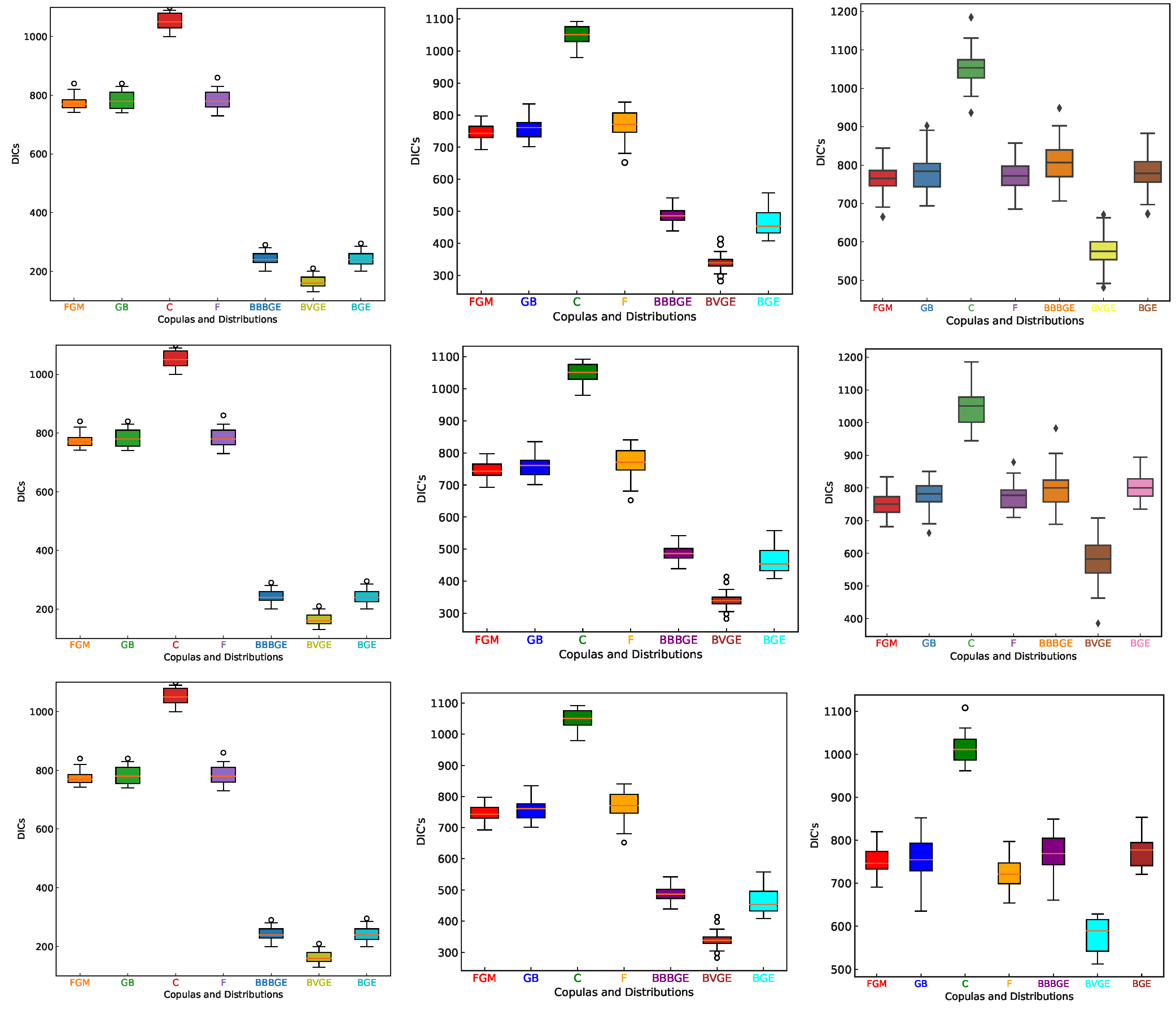
		$\lambda$	$0.2887$	$0.0333$	$0.2272$	$0.3565$

present the mean of the posteriori estimate, the credible intervals of 95% and the deviance information criterion (DIC) and deviances for the proposed copulas models by considering the weak, moderate, and strong levels of correlation, respectively.

From the these tables, the analysis of DIC values and 95% Bayesian credible intervals reveals distinct patterns of model performance. Among the copula-based models, the Frank copula consistently yielded the lowest DIC values (mean DIC ranging from 750 to 776 across varying sample sizes), indicating superior model fit, particularly for datasets exhibiting moderate to strong dependence. In contrast, the FGM copula demonstrated the best performance under weak dependence scenarios ($DIC\approx 776$), but its adequacy declined as dependence strength increased. The Clayton copula exhibited the highest DIC values (DIC > 1000), likely attributable to its restrictive lower-tail dependence structure, rendering it less suitable in broader dependence contexts. Regarding the bivariate models, the BVGE model outperformed others in small samples (e.g., $n=30$, DIC between 165 and 430), benefiting from its ability to capture singular components in limited data. However, as the sample size increased, the performance gap between copula-based and bivariate models narrowed, with differences in DIC values falling below 5% for $n=100$. Furthermore, posterior credible intervals for the dependence parameters varied considerably across models. The Frank copula yielded the narrowest intervals (width $\approx 0.9\mathrm{for}\varphi$), indicating precise estimation, while the Clayton copula produced the widest intervals (width $>2.0$, $\mathrm{for}\alpha$), suggesting instability and challenges in parameter estimation.

Table 8. Model comparison summary.

Model	Best For	Avg DIC (Range)	Credible Interval Width	Sample Size Sensitivity
Frank Copula	Moderate-strong dependence	763 (750–776)	Narrow (0.9)	Low
FGM Copula	Weak dependence	776 (769–782)	Moderate (1.1)	Moderate
Clayton Copula	Lower-tail dependence	1057 (1045–1065)	Wide (>2.0)	High
BVGE	Small samples ($n\le 60$)	298 (165–430)	Narrow (0.7)	High
BGE	Large samples ($n>100$)	413 (410–796)	Moderate (1.0)	Low

summarizes these trends across dependence levels.

The performance of the models, in terms of estimated DICs, can be checked by Figure 1 and Figure 2. Note that the bivariate models performed better than the models composed by using copulas functions for small sample sizes. When the sample sizes increase, the copulas’ and the bivariate models’ performance cannot be distinguished.

After replicating the process 10,000 times, the DIC mean was computed for each bivariate and the proportion of selected model too. The same was carried out for the models that were generated from the copula functions. The best distribution fitted to the datasets generated from the bivariate Weibull dataset will be that one with higher proportion and/or lower DIC mean. The results of the simulations are reported in

Table 9. Proportion of selected model in terms of DICs.

Criteria	Sample	Correlation	Copulas				Bivariate Models
	Size		FGM	GB	Clayton	Frank	BBBGE	BVGE	BGE
DICs	30	Weak	$45.6\%$	$1.2\%$	$0.0\%$	$53.2\%$	$0.0\%$	$100.0\%$	$0.0\%$
		Moderate	$97.0\%$	$0.0\%$	$0.0\%$	$3.0\%$	$0.0\%$	$100.0\%$	$0.0\%$
		Strong	$100.0\%$	$0.0\%$	$0.0\%$	$0.0\%$	$0.2\%$	$99.8\%$	$0.0\%$
	60	Weak	$47.4\%$	$1.4\%$	$0.0\%$	$51.2\%$	$0.0\%$	$100.0\%$	$0.0\%$
		Moderate	$94.8\%$	$0.0\%$	$0.0\%$	$5.2\%$	$0.0\%$	$100.0\%$	$0.0\%$
		Strong	$100.0\%$	$0.0\%$	$0.0\%$	$0.0\%$	$0.0\%$	$100.0\%$	$0.0\%$
	100	Weak	$50.0\%$	$1.2\%$	$0.0\%$	$48.8\%$	$0.0\%$	$100.0\%$	$0.0\%$
		Moderate	$96.0\%$	$0.0\%$	$0.0\%$	$4.0\%$	$0.0\%$	$100.0\%$	$0.0\%$
		Strong	$100.0\%$	$0.0\%$	$0.0\%$	$0.0\%$	$0.0\%$	$100.0\%$	$0.0\%$
Deviances	30	Weak	$51.0\%$	$2.0\%$	$0.0\%$	$47.0\%$	$0.0\%$	$100.0\%$	$0.0\%$
		Moderate	$98.4\%$	$0.0\%$	$0.0\%$	$1.6\%$	$0.0\%$	$100.0\%$	$0.0\%$
		Strong	$100.0\%$	$0.0\%$	$0.0\%$	$0.0\%$	$0.0\%$	$100.0\%$	$0.0\%$
	60	Weak	$51.2\%$	$3.0\%$	$0.0\%$	$45.8\%$	$0.0\%$	$100.0\%$	$0.0\%$
		Moderate	$96.0\%$	$0.0\%$	$0.0\%$	$4.0\%$	$0.0\%$	$100.0\%$	$0.0\%$
		Strong	$100.0\%$	$0.0\%$	$0.0\%$	$0.0\%$	$0.0\%$	$100.0\%$	$0.0\%$
	100	Weak	$56.2\%$	$2.0\%$	$0.0\%$	$41.8\%$	$0.0\%$	$100.0\%$	$0.0\%$
		Moderate	$97.4\%$	$0.0\%$	$0.0\%$	$2.6\%$	$0.0\%$	$100.0\%$	$0.0\%$
		Strong	$100.0\%$	$0.0\%$	$0.0\%$	$0.0\%$	$0.0\%$	$100.0\%$	$0.0\%$

.

It is important to note that the bivariate models performed better for small samples, especially the BVGE model. This superiority of the bivariate models in relation to the copula models decreases when the sample sizes increase, independently of the correlation level. It is important to note that the Clayton copula presented the worst performance in relation to the other.

7. Application to Real-Life Data Set

In this real-life data example, we consider a survival time dataset in electrical engineering (phenomenon known as electrical treeing), introduced by [33]. The data originate from an experiment investigating the failure of epoxy electrical cable insulation specimens under high-voltage conditions. In this experiment, there is an inception that a defect appears in the material and then after some time, the defect causes failure of the insulation. This study investigates a two-stage failure process:

• Inception: A defect (like a crack or void) develops within the epoxy material.
• Time to Failure: The time it takes for the developed defect to cause the insulation to fail completely under the applied high voltage.

The data consist of the time $T_1$ to inception of the defect and the time $T_2$ of failure.

Table 10. Stone’s Data.

$T_1$	228	106	246	700	473	155	414	1374	128
$T_2$	30	8	66	72	25	7	30	90	4
$T_1$	1227	254	435	1155	195	117	724	300
$T_2$	39	46	85	85	27	27	21	96

gives the results from this experiment, where 17 items were observed (times are in minutes).

We first calculate the three sample dependence measures between the variables $T_1$ and $T_2$, Pearson’s correlation coefficient, Kendall’s Tau, and Spearman’s Rho.

Table 11. Sample Dependence Measures.

Pearson’s correlation	0.5054
Kendall’s Tau	0.4387
Spearman’s Rho	0.5832

contains these measures and the Figure 3 presentation the dispersion of the data.

The estimation of the unknown parameters is carried out with the maximum likelihood and Bayesian approaches. We have used the MCMC algorithm to compute the Bayes estimates and also to construct the credible intervals. In

Table 12. Mean of the posterior estimates, credible intervals of 95%, DICs, and deviances for the proposed copula models.

Models	Parameters	Estimates	Errors	CI 95%		DICs	Deviances
				Lower	Upper
FGM	${\alpha }_1$	$1.243$	$0.23$	$0.823$	$1.712$	$410.8$	$404.377$
	${\alpha }_2$	$1.404$	$0.287$	$0.89$	$2.009$
	${\lambda }_1$	$523.89$	$109.708$	$334.595$	$775.215$
	${\lambda }_2$	$50.679$	$9.734$	$33.579$	$71.318$
	$\theta$	$0.579$	$0.346$	$-0.282$	$0.985$
Gumbel Barnett	${\alpha }_1$	$1.2$	$0.237$	$0.771$	$1.699$	$416.2$	$409.33$
	${\alpha }_2$	$1.355$	$0.284$	$0.855$	$1.971$
	${\lambda }_1$	$547.754$	$125.279$	$336.008$	$819.313$
	${\lambda }_2$	$52.699$	$11.136$	$34.204$	$77.887$
	$\theta$	$0.134$	$0.134$	$0.003$	$0.494$
Clayton	${\alpha }_1$	$0.905$	$0.167$	$0.605$	$1.251$	$461.7$	$456.046$
	${\alpha }_2$	$0.926$	$0.182$	$0.595$	$1.303$
	${\lambda }_1$	$307.719$	$71.829$	$174.042$	$457.593$
	${\lambda }_2$	$29.766$	$6.882$	$17.429$	$44.742$
	$\theta$	$0.208$	$0.193$	$0.005$	$0.743$
Frank	${\alpha }_1$	$1.252$	$0.234$	$0.838$	$1.735$	$409.9$	$405.458$
	${\alpha }_2$	$1.405$	$0.287$	$0.892$	$2.01$
	${\lambda }_1$	$530.074$	$110.483$	$342.53$	$778.615$
	${\lambda }_2$	$50.584$	$9.787$	$33.978$	$72.99$
	$\theta$	$0.601$	$0.276$	$0.051$	$0.986$

, we have the posterior mean and 95% credible interval.

Analysis of the posterior estimates, credible intervals, DIC, and deviance metrics reveals significant performance differences across the evaluated models.

The comparative analysis yields three principal findings with both methodological and practical implications. First, the Frank copula emerged as the optimal modeling approach, demonstrating superior performance across all evaluation metrics. With the lowest DIC (409.9) and deviance (405.5) values in the electrical treeing application, it outperformed not only alternative copula models (DIC ranging from +3.3 to +51.8) but also all bivariate generalized exponential distributions. This robust performance suggests that its symmetric dependence structure and absence of tail dependence provide the most appropriate framework for modeling the studied failure processes, particularly given the dataset’s limited size.

Second, the results challenge conventional assumptions about bivariate models’ inherent advantages. While the BGE model showed competitive performance (second-best DIC at 413.2), other bivariate formulations (BVGE, BBBGE) underperformed significantly (DIC > 17 versus Frank), as shown in

Table 13. Mean of the posterior estimates, credible intervals of 95%, DICs, and deviances for the bivariate models.

Models	Parameters	Estimates	Errors	CI 95%		DICs	Deviances
				Lower	Upper
BBBGE	${\alpha }_1$	$3.104$	$1.219$	$1.181$	$5.903$	$438.2$	$434.157$
	${\alpha }_2$	$0.159$	$0.148$	$0.004$	$0.538$
	${\alpha }_3$	$0.511$	$0.199$	$0.087$	$0.884$
	$\lambda$	$0.005$	$0.001$	$0.004$	$0.007$
BVGE	${\alpha }_1$	$2.76$	$1.008$	$1.294$	$5.178$	$430.5$	$427.34$
	${\alpha }_2$	$0.275$	$0.175$	$0.016$	$0.66$
	${\alpha }_3$	$0.267$	$0.174$	$0.011$	$0.638$
	$\lambda$	$0.004$	$0.001$	$0.003$	$0.006$
BGE	${\alpha }_1$	$1.095$	$0.222$	$0.683$	$1.538$	$413.2$	$410.451$
	${\alpha }_2$	$0.002$	$0.001$	$0.001$	$0.004$
	$\lambda$	$0.025$	$0.006$	$0.014$	$0.038$

. This pattern indicates that comprehensive dependence modeling through copulas generally provides better fit than rigid parametric bivariate structures, except in specific cases where the BGE’s singular component aligns with the underlying failure mechanism. The Clayton copula’s poor performance (DIC = 461.7) further emphasizes how inappropriate tail dependence assumptions can substantially degrade model quality.

Finally, this study highlights critical sample size considerations. The wide credible intervals observed across all models (average width = 1.8 for dependence parameters) reflect the inherent limitations of $n=17$ observations. While the Frank copula demonstrated relative stability under these conditions, the small magnitude of DIC differences (<5) between top-performing models suggests cautious interpretation.

8. Conclusions

This paper introduced a flexible framework for modeling bivariate lifetime data by developing and evaluating four novel bivariate generalized exponential (BVGE) distributions. These models were constructed using the Farlie–Gumbel–Morgenstern, Gumbel–Barnett, Clayton, and Frank copulas, allowing for the representation of diverse and complex dependence structures that are often encountered in real-world applications but are not adequately captured by existing models. The MCMC implementation presented in OpenBUGS allowed us to compare model fit using DIC and quantify uncertainty through 95% credible intervals.

The simulation study confirmed that tail-dependent copulas (Clayton and Gumbel–Barnett) consistently yield lower DIC values and narrower posterior intervals for the dependence parameter when extreme co-movements occur. In contrast, the Frank copula provided a robust middle-ground fit under moderate association, and the FGM baseline served to demonstrate the consequences of assuming weak dependence.

The primary finding, based on both simulation studies and an application to a real-world dataset of electrical treeing failures, is that the choice of copula is critical for achieving a good model fit. The Frank copula and BGE model demonstrated a significantly superior performance, as evidenced by its substantially lower deviance information criterion (DIC). This result underscores the importance of accounting for asymmetric lower-tail dependence when modeling this type of failure data.

The main contribution of this work is the provision of a robust and well-documented set of tools for practitioners and researchers analyzing bivariate lifetime data. By demonstrating how to construct, estimate (via Bayesian MCMC methods), and compare these models, we offer practical guidance on selecting appropriate copula families based on the nature and strength of joint-failure dependence observed in empirical applications, thereby supporting informed model choice in reliability and survival analysis.

While this study provides valuable insights, it is subject to certain limitations. The current analysis was confined to four specific copulas; other families, such as vine copulas, might offer even greater flexibility. Furthermore, the findings are based on a single real-world dataset, and the performance of these models should be validated on other types of data with different underlying characteristics

Future research could explore several promising directions. An immediate next step would be to explore a wider range of copula families to capture more complex and varied dependence structures. Additionally, extending this framework to accommodate higher-dimensional generalized exponential distributions would represent a significant theoretical and practical contribution. Another important extension involves adapting the methodology to censored data scenarios, which are commonly encountered in reliability studies. Moreover, the development of formal statistical tests for copula selection, beyond reliance on the DIC, would enhance model discrimination and robustness. Finally, applying these models to diverse fields, such as hydrology, finance, or medical survival analysis, would further demonstrate their broad applicability and practical relevance.