
Optimum Progressive Data Analysis and Bayesian Inference for Unified Progressive Hybrid INH Censoring with Applications to Diamonds and Gold


Abstract
1. Introduction
2. The UPH-CT1 Plan
3. Likelihood Inference
3.1. Maximum Likelihood Estimators
3.2. Approximate Interval Estimators
4. Bayesian Inference
| Algorithm 1 MCMC Generation Steps |
|
5. Monte Carlo Comparisons
5.1. Simulation Scenarios
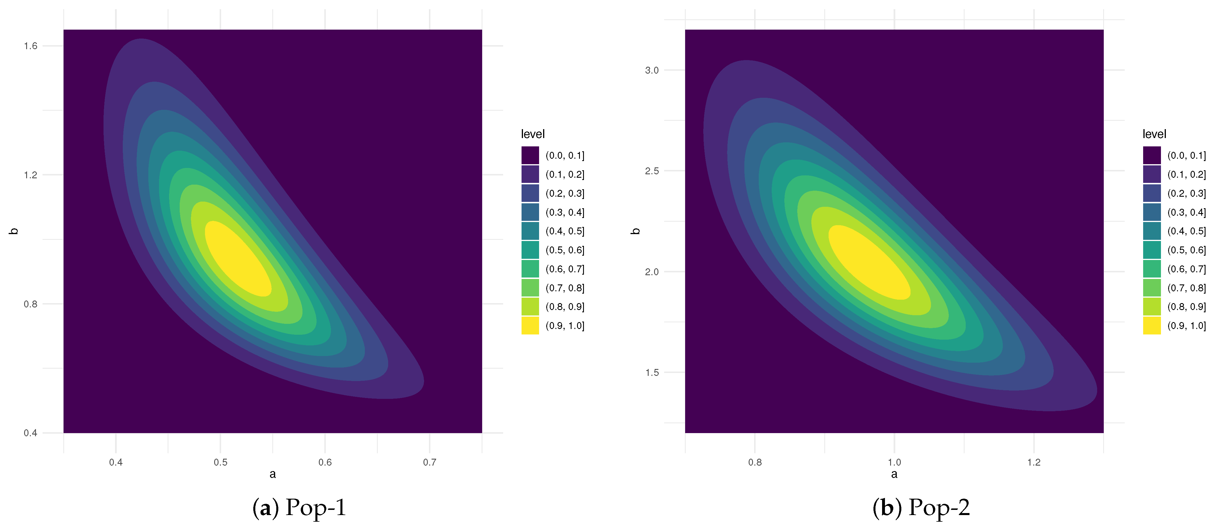
- For Pop-1:INH(0.5, 1):
- –
- Prior A[PA]: and ,
- –
- Prior B[PB]: and ,
- For Pop-2:INH(1, 2):
- –
- Prior A[PA]: and ,
- –
- Prior B[PB]: and ,
| Algorithm 2 UPH-CT1 generation steps |
|
5.2. Simulation Results and Discussion
- The obtained estimates of a, b, , and consistently demonstrate enhanced performance, yielding results of greater statistical efficiency.
- With increasing n (r or m), both the Bayesian and classical approaches produce stable and accurate estimates for a, b, , and . A similar improvement in estimation quality is evident when the total number of removals is minimized.
- As the threshold values of grow, we observe that the RMSE, ARAB, and AIL values for all parameters and reliability metrics tend to decrease, while the associated CP values tend to increase.
- In both the Pop-1 and Pop-2 groups, Bayesian estimation using PB outperforms PA, as the former exhibits reduced prior variance, resulting in more stable and reliable posterior summaries for all parameters.
- Bayesian estimators of a, b, , and calculated by the Pop-1 and Pop-2 groups provide superior results compared to their frequentist counterparts, largely due to the incorporation of gamma prior information.
- When the true values of INH increased, we noted for the Pop-1 and Pop-2 groups that:
- –
- The RMSE and ARAB associated with the frequentist (or Bayesian) estimates of a, b, , and increase.
- –
- The AILs derived from ACI (or BCI) procedures also correspondingly increase; conversely, their CPs tend to decrease.
- Comparing the three censoring designs reported in Table 1, for both Pop-1 and Pop-2 groups it can be noted that the most efficient estimates of a and are obtained using the right P-CT2 ‘Design [C]’, while those of of are obtained using the left P-CT2 ‘Design [A]’ and those of b are obtained using the middle P-CT2 ‘Design B]’.
- In summary, when analyzing data generated from the UPH-CT1 strategy, the Bayesian approach based on Markovian iterations is strongly recommended for precise inference on INH model parameters and associated reliability measures.
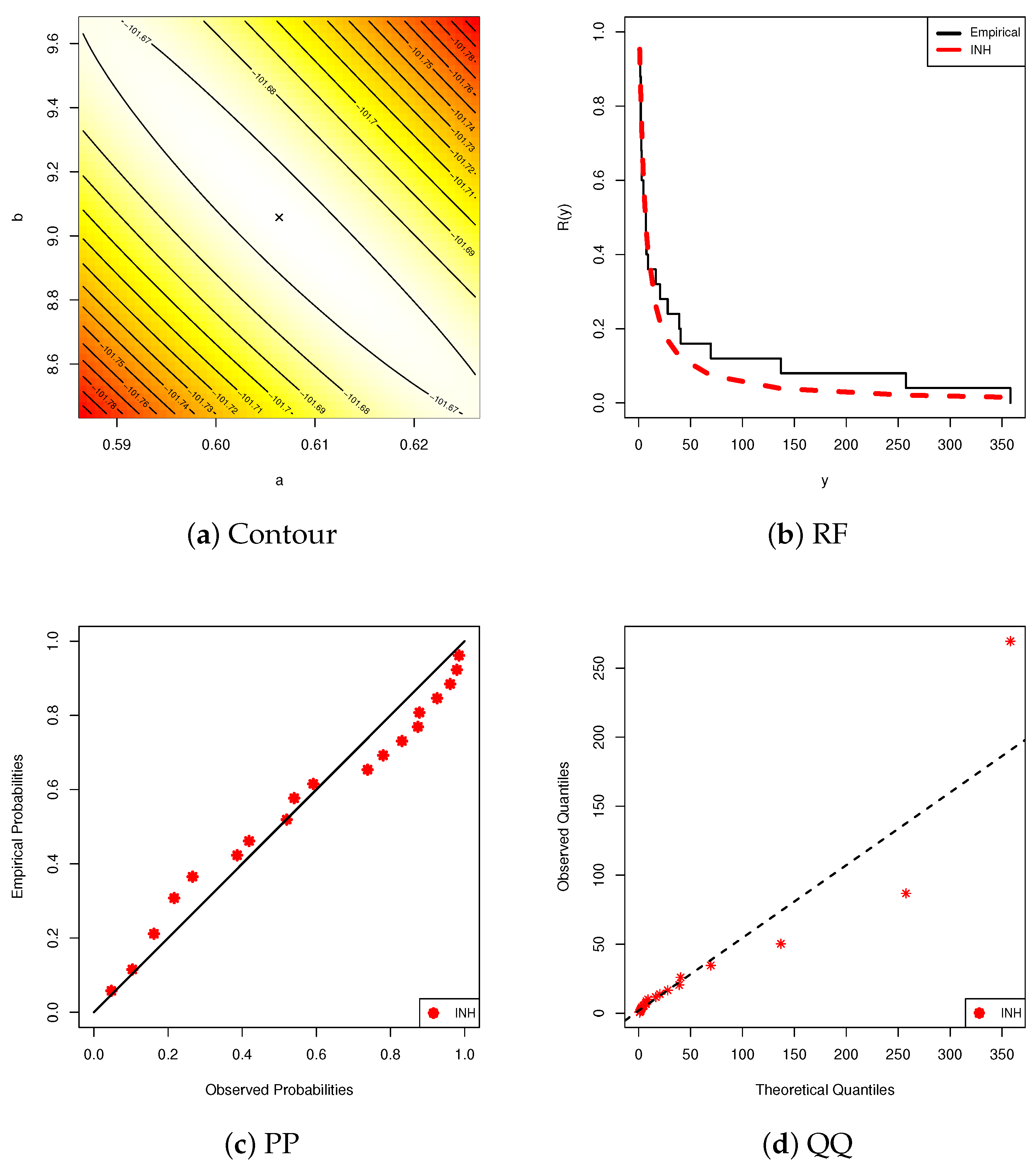
6. Rare Minerals Data Analysis
6.1. Diamond Data
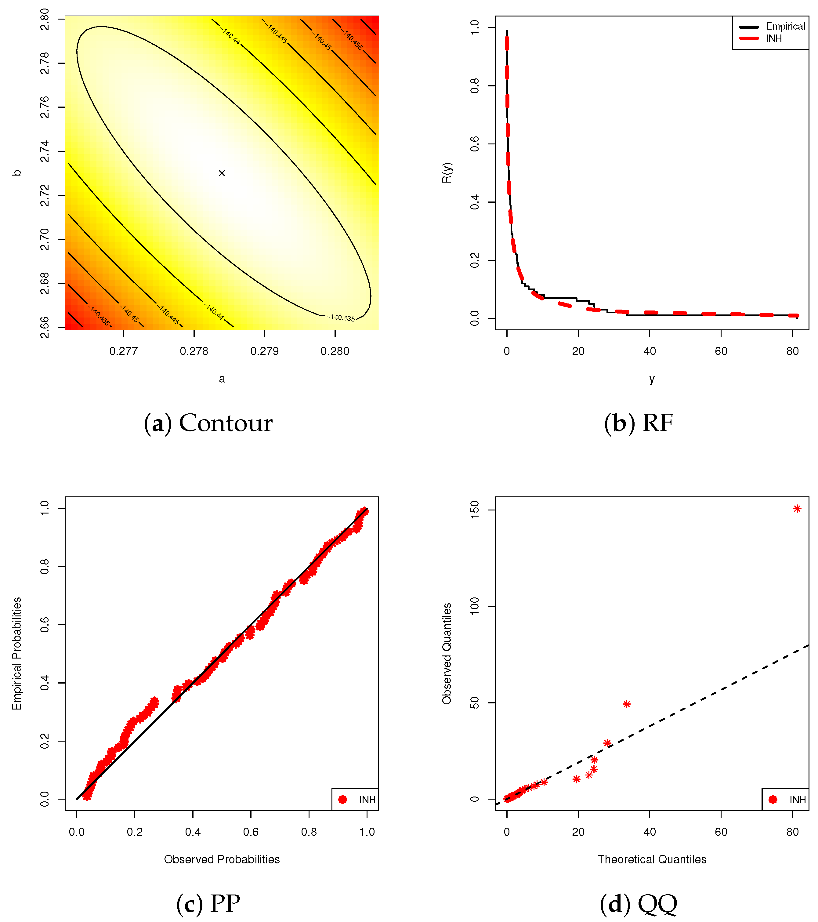
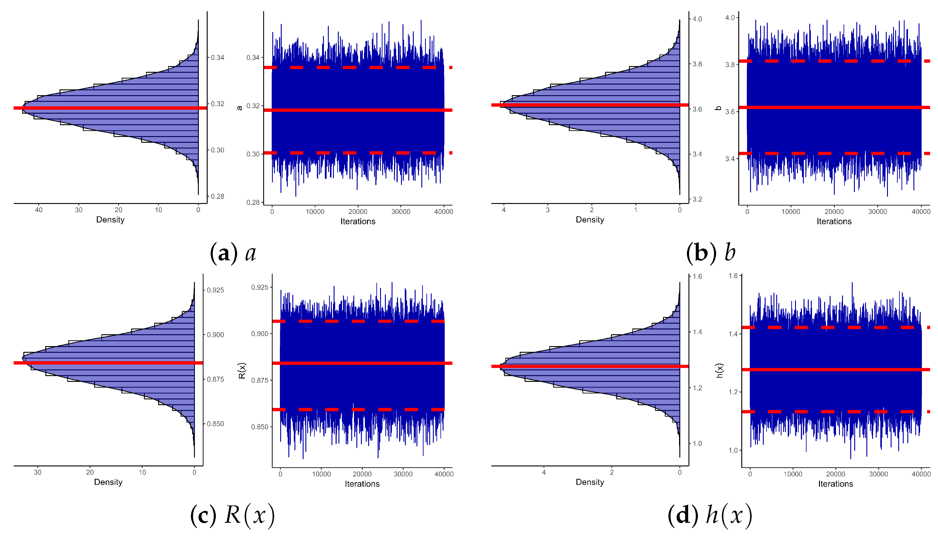
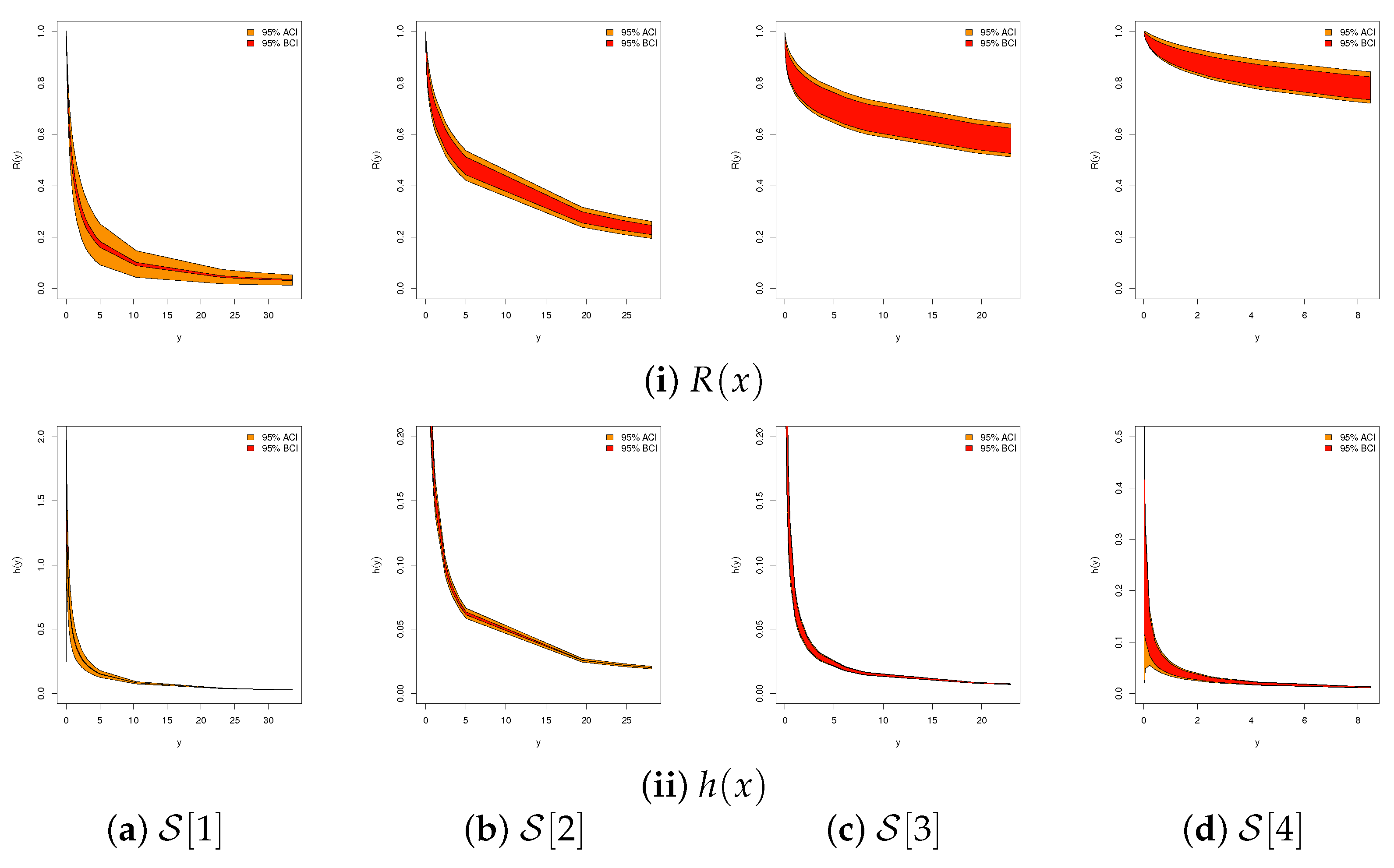
6.2. Gold Data
7. Optimal Progressive Design
- Maximizing the trace of observed FI items, denoted by , as
- Minimizing the trace of observed VC items , denoted by , as
- Minimizing the determinant of observed VC items , denoted by , as
- Minimizing the MLE of the logarithm of th quantile, denoted by , aswhere and such that
- (i)
- From the Diamond Data:
- According to criteria , the left P-CT2 (used in ) is more optimal than the others;
- According to criteria , the right P-CT2 (used in ) is more optimal than the others.
- (ii)
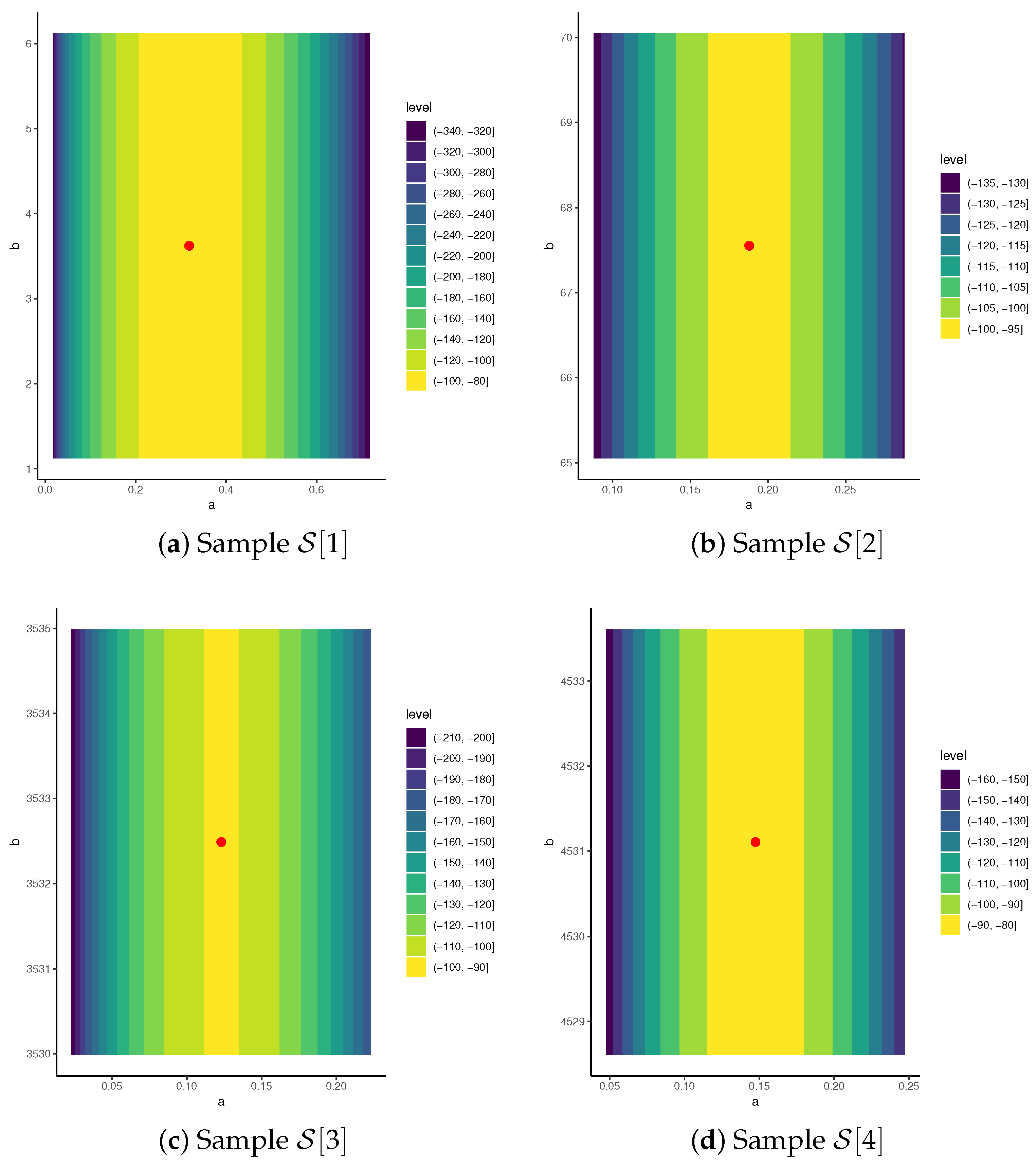
- From the Gold Data:
- According to criterion , the right P-CT2 (used in ) is more optimal than the others;
- According to criteria , the left P-CT2 (used in ) is more optimal than the others.
- (1)
- It demonstrates considerable adaptability, particularly in scenarios where the termination of the test is primarily driven by the number of observed failures;
- (2)
- It allows researchers to maintain control over the experiment’s duration;
- (3)
- It facilitates the extraction of reliable and informative estimates for both the reliability function and the hazard rate without the need to observe the entire sample, offering significant reductions in time, cost, and manpower.
8. Concluding Remarks
Author Contributions
Funding
Data Availability Statement
Acknowledgments
Conflicts of Interest
Appendix A
References
- Childs, A.; Chandrasekar, B.; Balakrishnan, N.; Kundu, D. Exact likelihood inference based on Type-I and Type-II hybrid censored samples from the exponential distribution. Ann. Inst. Stat. Math. 2003, 55, 319–330. [Google Scholar] [CrossRef]
- Chandrasekar, B.; Childs, A.; Balakrishnan, N. Exact likelihood inference for the exponential distribution under generalized Type-I and Type-II hybrid censoring. Nav. Res. Logist. 2004, 51, 994–1004. [Google Scholar] [CrossRef]
- Balakrishnan, N.; Rasouli, A.; Farsipour, N.S. Exact likelihood inference based on an unified hybrid censored sample from the exponential distribution. J. Stat. Comput. Simul. 2008, 78, 475–488. [Google Scholar] [CrossRef]
- Balakrishnan, N.; Cramer, E. The Art of Progressive Censoring. Statistics for Industry and Technology; Springer Birkhäuser: New York, NY, USA, 2014. [Google Scholar]
- Górny, J.; Cramer, E. Modularization of hybrid censoring schemes and its application to unified progressive hybrid censoring. Metrika 2018, 81, 173–210. [Google Scholar] [CrossRef]
- Nadarajah, S.; Haghighi, F. An extension of the exponential distribution. Statistics 2011, 45, 543–558. [Google Scholar] [CrossRef]
- Tahir, M.H.; Cordeiro, G.M.; Ali, S.; Dey, S.; Manzoor, A. The inverted Nadarajah–Haghighi distribution: Estimation methods and applications. J. Stat. Comput. Simul. 2018, 88, 2775–2798. [Google Scholar] [CrossRef]
- Elshahhat, A.; Rastogi, M.K. Estimation of parameters of life for an inverted Nadarajah–Haghighi distribution from Type-II progressively censored samples. J. Indian Soc. Probab. Stat. 2021, 22, 113–154. [Google Scholar] [CrossRef]
- Elshahhat, A.; Mohammed, H.S.; Abo-Kasem, O.E. Reliability inferences of the inverted NH parameters via generalized type-II progressive hybrid censoring with applications. Symmetry 2022, 14, 2379. [Google Scholar] [CrossRef]
- Abushal, T.A. Statistical inference for Nadarajah-Haghighi distribution under unified hybrid censored competing risks data. Heliyon 2024, 10, e26794. [Google Scholar] [CrossRef] [PubMed]
- Abushal, T.A.; AL-Zaydi, A.M. Statistical inference of inverted Nadarajah–Haghighi distribution under type-II generalized hybrid censoring competing risks data. J. Eng. Math. 2024, 144, 24. [Google Scholar] [CrossRef]
- Azimi, R.; Esmailian, M. Bayesian Inference for Nadarajah-Haghighi Distribution Under Progressively Type-II Censored Data. Thail. Stat. 2025, 23, 279–297. [Google Scholar]
- Lone, S.A.; Panahi, H.; Anwar, S.; Shahab, S. Estimations and optimal censoring schemes for the unified progressive hybrid gamma-mixed Rayleigh distribution. Electron. Res. Arch. 2023, 31, 4729–4752. [Google Scholar] [CrossRef]
- Anwar, S.; Lone, S.A.; Khan, A.; Almutlak, S. Stress-strength reliability estimation for the inverted exponentiated Rayleigh distribution under unified progressive hybrid censoring with application. Electron. Res. Arch. 2023, 31, 4011–4033. [Google Scholar] [CrossRef]
- Bayoud, H.A.; Almathkour, F.B.; Raqab, M.Z. Advanced inference techniques for two-parameter Topp-Leone models under unified progressively hybrid censoring. Commun. -Stat.-Simul. Comput. 2024, 1–24. [Google Scholar] [CrossRef]
- Dutta, S.; Kayal, S. Estimation and prediction for Burr type III distribution based on unified progressive hybrid censoring scheme. J. Appl. Stat. 2024, 51, 1–33. [Google Scholar] [CrossRef] [PubMed]
- Dey, S.; Elshahhat, A.; Nassar, M. Analysis of progressive Type-II censored gamma distribution. Comput. Stat. 2023, 38, 481–508. [Google Scholar] [CrossRef]
- Henningsen, A.; Toomet, O. maxLik: A package for maximum likelihood estimation in R. Comput. Stat. 2011, 26, 443–458. [Google Scholar] [CrossRef]
- Plummer, M.; Best, N.; Cowles, K.; Vines, K. CODA: Convergence diagnosis and output analysis for MCMC. R News 2006, 6, 7–11. [Google Scholar]
- Kundu, D. Bayesian inference and life testing plan for the Weibull distribution in presence of progressive censoring. Technometrics 2008, 50, 144–154. [Google Scholar] [CrossRef]
- Maurya, S.K.; Goyal, T. A New Decreasing Failure Rate Distribution and Its Real Life Application. Int. J. Stat. Reliab. Eng. 2023, 10. Available online: https://www.researchgate.net/publication/380431739_A_New_Decreasing_Failure_Rate_Distribution_and_Its_Real_Life_Application (accessed on 20 July 2025).
- Alqasem, O.A.; Nassar, M.; Abd Elwahab, M.E.; Elshahhat, A. A new inverted Pham distribution for data modeling of mechanical components and diamond in South-West Africa. Phys. Scr. 2024, 99, 115268. [Google Scholar] [CrossRef]
- Ng, H.K.T.; Chan, P.S.; Balakrishnan, N. Optimal progressive censoring plans for the Weibull distribution. Technometrics 2004, 46, 470–481. [Google Scholar] [CrossRef]
- Pradhan, B.; Kundu, D. Inference and optimal censoring schemes for progressively censored Birnbaum–Saunders distribution. J. Stat. Plan. Inference 2013, 143, 1098–1108. [Google Scholar] [CrossRef]
- Sen, T.; Tripathi, Y.M.; Bhattacharya, R. Statistical inference and optimum life testing plans under Type-II hybrid censoring scheme. Ann. Data Sci. 2018, 5, 679–708. [Google Scholar] [CrossRef]
- Ashour, S.K.; El-Sheikh, A.A.; Elshahhat, A. Inferences and optimal censoring schemes for progressively first-failure censored Nadarajah-Haghighi distribution. Sankhyā A Indian J. Stat. 2022, 84, 885–923. [Google Scholar] [CrossRef]
- Nassar, M.; Elshahhat, A. Estimation procedures and optimal censoring schemes for an improved adaptive progressively type-II censored Weibull distribution. J. Appl. Stat. 2024, 51, 1664–1688. [Google Scholar] [CrossRef] [PubMed]


| R | Design | ||
|---|---|---|---|
| 20[25%] | 20[50%] | [A] | |
| [B] | |||
| [C] | |||
| 20[50%] | 20[75%] | [A] | |
| [B] | |||
| [C] | |||
| 40[25%] | 40[50%] | [A] | |
| [B] | |||
| [C] | |||
| 40[50%] | 40[75%] | [A] | |
| [B] | |||
| [C] | |||
| 80[25%] | 80[50%] | [A] | |
| [B] | |||
| [C] | |||
| 80[50%] | 80[75%] | [A] | |
| [B] | |||
| [C] |
| R | MLE | Bayes[PA] | Bayes[PB] | MLE | Bayes[PA] | Bayes[PB] | ||||||||||||||
|---|---|---|---|---|---|---|---|---|---|---|---|---|---|---|---|---|---|---|---|---|
| Pop-1 | ||||||||||||||||||||
| 20[25%] | 20[50%] | [A] | 0.765 | 1.950 | 1.789 | 0.445 | 0.121 | 0.188 | 0.430 | 0.113 | 0.174 | 0.888 | 1.678 | 1.724 | 0.440 | 0.116 | 0.178 | 0.433 | 0.105 | 0.166 |
| [B] | 0.648 | 2.157 | 1.929 | 0.438 | 0.124 | 0.196 | 0.426 | 0.116 | 0.179 | 0.721 | 1.779 | 1.898 | 0.443 | 0.122 | 0.183 | 0.427 | 0.112 | 0.176 | ||
| [C] | 0.866 | 1.732 | 1.635 | 0.439 | 0.112 | 0.175 | 0.430 | 0.103 | 0.164 | 0.763 | 1.643 | 1.481 | 0.437 | 0.108 | 0.171 | 0.430 | 0.099 | 0.163 | ||
| 20[50%] | 20[75%] | [A] | 0.741 | 1.657 | 1.330 | 0.475 | 0.100 | 0.165 | 0.488 | 0.096 | 0.158 | 0.604 | 1.318 | 1.280 | 0.474 | 0.097 | 0.164 | 0.489 | 0.095 | 0.156 |
| [B] | 0.692 | 1.679 | 1.480 | 0.472 | 0.105 | 0.171 | 0.481 | 0.097 | 0.161 | 0.859 | 1.464 | 1.394 | 0.475 | 0.100 | 0.167 | 0.483 | 0.097 | 0.159 | ||
| [C] | 0.642 | 1.609 | 1.268 | 0.475 | 0.098 | 0.165 | 0.488 | 0.092 | 0.153 | 0.582 | 1.283 | 1.235 | 0.472 | 0.095 | 0.160 | 0.487 | 0.090 | 0.150 | ||
| 40[25%] | 40[50%] | [A] | 0.670 | 1.466 | 0.540 | 0.554 | 0.091 | 0.143 | 0.581 | 0.087 | 0.133 | 0.655 | 1.226 | 0.458 | 0.538 | 0.088 | 0.143 | 0.569 | 0.085 | 0.132 |
| [B] | 0.714 | 1.528 | 0.551 | 0.563 | 0.097 | 0.161 | 0.587 | 0.091 | 0.145 | 0.680 | 1.264 | 0.484 | 0.554 | 0.092 | 0.146 | 0.576 | 0.088 | 0.139 | ||
| [C] | 0.619 | 1.052 | 0.495 | 0.539 | 0.090 | 0.142 | 0.574 | 0.083 | 0.131 | 0.617 | 1.018 | 0.449 | 0.543 | 0.088 | 0.142 | 0.577 | 0.082 | 0.130 | ||
| 40[50%] | 40[75%] | [A] | 0.719 | 0.745 | 0.392 | 0.509 | 0.088 | 0.141 | 0.532 | 0.082 | 0.128 | 0.674 | 0.528 | 0.347 | 0.511 | 0.087 | 0.140 | 0.535 | 0.081 | 0.128 |
| [B] | 0.694 | 0.907 | 0.466 | 0.506 | 0.089 | 0.142 | 0.536 | 0.082 | 0.130 | 0.619 | 0.710 | 0.428 | 0.498 | 0.087 | 0.142 | 0.532 | 0.082 | 0.129 | ||
| [C] | 0.643 | 0.324 | 0.357 | 0.504 | 0.087 | 0.141 | 0.534 | 0.081 | 0.125 | 0.671 | 0.321 | 0.341 | 0.498 | 0.087 | 0.139 | 0.531 | 0.081 | 0.124 | ||
| 80[25%] | 80[50%] | [A] | 0.585 | 0.145 | 0.201 | 0.511 | 0.081 | 0.135 | 0.558 | 0.080 | 0.123 | 0.542 | 0.137 | 0.192 | 0.501 | 0.080 | 0.125 | 0.543 | 0.079 | 0.120 |
| [B] | 0.655 | 0.160 | 0.219 | 0.532 | 0.086 | 0.140 | 0.576 | 0.081 | 0.123 | 0.549 | 0.146 | 0.203 | 0.511 | 0.081 | 0.131 | 0.564 | 0.080 | 0.121 | ||
| [C] | 0.543 | 0.131 | 0.186 | 0.498 | 0.080 | 0.124 | 0.553 | 0.076 | 0.121 | 0.547 | 0.129 | 0.180 | 0.502 | 0.077 | 0.124 | 0.556 | 0.073 | 0.119 | ||
| 80[50%] | 80[75%] | [A] | 0.561 | 0.103 | 0.144 | 0.453 | 0.072 | 0.120 | 0.494 | 0.067 | 0.111 | 0.515 | 0.100 | 0.143 | 0.452 | 0.072 | 0.112 | 0.464 | 0.062 | 0.106 |
| [B] | 0.591 | 0.103 | 0.144 | 0.452 | 0.075 | 0.123 | 0.546 | 0.069 | 0.115 | 0.516 | 0.100 | 0.143 | 0.436 | 0.073 | 0.116 | 0.456 | 0.064 | 0.110 | ||
| [C] | 0.571 | 0.100 | 0.143 | 0.451 | 0.072 | 0.111 | 0.426 | 0.064 | 0.106 | 0.516 | 0.098 | 0.141 | 0.435 | 0.064 | 0.110 | 0.450 | 0.062 | 0.099 | ||
| Pop-2 | ||||||||||||||||||||
| 20[25%] | 20[50%] | [A] | 1.642 | 2.320 | 1.918 | 1.278 | 0.361 | 0.303 | 1.069 | 0.180 | 0.153 | 1.489 | 1.946 | 1.866 | 1.264 | 0.359 | 0.303 | 1.068 | 0.178 | 0.148 |
| [B] | 1.874 | 2.424 | 2.093 | 1.274 | 0.374 | 0.317 | 1.056 | 0.185 | 0.153 | 1.641 | 1.979 | 1.952 | 1.277 | 0.360 | 0.304 | 1.056 | 0.178 | 0.149 | ||
| [C] | 1.470 | 1.928 | 1.894 | 1.282 | 0.358 | 0.302 | 1.082 | 0.176 | 0.148 | 1.533 | 1.921 | 1.645 | 1.296 | 0.355 | 0.290 | 1.085 | 0.175 | 0.147 | ||
| 20[50%] | 20[75%] | [A] | 1.641 | 1.879 | 1.891 | 1.037 | 0.344 | 0.289 | 0.873 | 0.175 | 0.137 | 1.483 | 1.781 | 1.500 | 1.031 | 0.337 | 0.284 | 0.876 | 0.174 | 0.134 |
| [B] | 1.385 | 1.275 | 0.909 | 1.035 | 0.196 | 0.155 | 0.920 | 0.141 | 0.116 | 1.177 | 1.111 | 0.553 | 1.018 | 0.196 | 0.154 | 0.920 | 0.139 | 0.114 | ||
| [C] | 1.556 | 1.743 | 1.744 | 1.025 | 0.339 | 0.267 | 0.871 | 0.175 | 0.133 | 1.381 | 1.492 | 1.277 | 1.017 | 0.318 | 0.251 | 0.866 | 0.168 | 0.130 | ||
| 40[25%] | 40[50%] | [A] | 1.440 | 1.628 | 1.189 | 1.061 | 0.264 | 0.170 | 0.949 | 0.152 | 0.121 | 1.294 | 1.378 | 1.167 | 1.054 | 0.210 | 0.163 | 0.954 | 0.152 | 0.124 |
| [B] | 1.306 | 1.725 | 1.679 | 1.078 | 0.297 | 0.177 | 0.953 | 0.161 | 0.128 | 1.434 | 1.415 | 1.223 | 1.054 | 0.229 | 0.166 | 0.941 | 0.158 | 0.126 | ||
| [C] | 1.252 | 1.472 | 1.175 | 1.045 | 0.250 | 0.166 | 0.959 | 0.147 | 0.120 | 1.190 | 1.323 | 1.110 | 1.053 | 0.208 | 0.161 | 0.953 | 0.145 | 0.120 | ||
| 40[50%] | 40[75%] | [A] | 1.482 | 1.870 | 1.787 | 1.025 | 0.341 | 0.288 | 0.874 | 0.175 | 0.137 | 1.538 | 1.512 | 1.427 | 1.017 | 0.337 | 0.283 | 0.866 | 0.173 | 0.132 |
| [B] | 1.295 | 1.337 | 1.157 | 1.041 | 0.242 | 0.165 | 0.915 | 0.144 | 0.119 | 1.355 | 1.279 | 1.067 | 1.011 | 0.205 | 0.161 | 0.911 | 0.143 | 0.118 | ||
| [C] | 1.134 | 1.314 | 1.047 | 1.030 | 0.232 | 0.164 | 0.918 | 0.142 | 0.118 | 1.249 | 1.238 | 0.990 | 1.017 | 0.203 | 0.159 | 0.915 | 0.141 | 0.116 | ||
| 80[25%] | 80[50%] | [A] | 1.236 | 1.007 | 0.497 | 1.274 | 0.183 | 0.149 | 1.121 | 0.125 | 0.104 | 1.431 | 0.910 | 0.438 | 1.282 | 0.168 | 0.141 | 1.119 | 0.123 | 0.105 |
| [B] | 1.251 | 1.202 | 0.586 | 1.273 | 0.195 | 0.151 | 1.121 | 0.127 | 0.110 | 1.238 | 1.023 | 0.507 | 1.240 | 0.176 | 0.142 | 1.115 | 0.124 | 0.108 | ||
| [C] | 1.299 | 0.748 | 0.419 | 1.257 | 0.180 | 0.143 | 1.116 | 0.123 | 0.104 | 1.247 | 0.688 | 0.370 | 1.278 | 0.157 | 0.139 | 1.114 | 0.122 | 0.102 | ||
| 80[50%] | 80[75%] | [A] | 1.123 | 0.525 | 0.282 | 0.995 | 0.131 | 0.127 | 0.951 | 0.122 | 0.101 | 1.125 | 0.495 | 0.281 | 0.995 | 0.131 | 0.105 | 0.951 | 0.122 | 0.101 |
| [B] | 1.112 | 0.502 | 0.279 | 0.991 | 0.128 | 0.110 | 0.942 | 0.122 | 0.100 | 1.126 | 0.457 | 0.269 | 0.975 | 0.125 | 0.101 | 0.941 | 0.121 | 0.099 | ||
| [C] | 1.106 | 0.488 | 0.267 | 0.983 | 0.126 | 0.108 | 0.945 | 0.121 | 0.099 | 1.121 | 0.436 | 0.263 | 0.948 | 0.122 | 0.100 | 0.931 | 0.118 | 0.098 | ||
| R | MLE | Bayes[PA] | Bayes[PB] | MLE | Bayes[PA] | Bayes[PB] | ||||||||||||||
|---|---|---|---|---|---|---|---|---|---|---|---|---|---|---|---|---|---|---|---|---|
| Pop-1 | ||||||||||||||||||||
| 20[25%] | 20[50%] | [A] | 1.014 | 1.661 | 0.924 | 0.899 | 0.436 | 0.341 | 0.907 | 0.341 | 0.297 | 1.143 | 1.651 | 0.891 | 0.865 | 0.424 | 0.337 | 0.895 | 0.340 | 0.296 |
| [B] | 1.141 | 1.505 | 0.848 | 0.922 | 0.398 | 0.328 | 0.911 | 0.337 | 0.288 | 1.044 | 1.465 | 0.774 | 0.955 | 0.387 | 0.311 | 0.931 | 0.325 | 0.280 | ||
| [C] | 1.089 | 1.609 | 0.890 | 0.873 | 0.409 | 0.336 | 0.902 | 0.332 | 0.289 | 1.074 | 1.492 | 0.850 | 0.907 | 0.389 | 0.321 | 0.877 | 0.329 | 0.285 | ||
| 20[50%] | 20[75%] | [A] | 0.989 | 1.144 | 0.719 | 1.031 | 0.396 | 0.324 | 0.878 | 0.317 | 0.276 | 1.018 | 1.143 | 0.714 | 1.004 | 0.380 | 0.309 | 0.870 | 0.283 | 0.239 |
| [B] | 0.971 | 1.036 | 0.673 | 1.041 | 0.386 | 0.305 | 0.879 | 0.282 | 0.228 | 1.017 | 0.995 | 0.653 | 1.069 | 0.366 | 0.297 | 0.884 | 0.266 | 0.227 | ||
| [C] | 0.956 | 1.042 | 0.679 | 1.046 | 0.394 | 0.313 | 0.878 | 0.298 | 0.241 | 0.995 | 1.034 | 0.676 | 1.043 | 0.374 | 0.298 | 0.873 | 0.273 | 0.234 | ||
| 40[25%] | 40[50%] | [A] | 1.060 | 0.874 | 0.615 | 1.017 | 0.365 | 0.296 | 0.819 | 0.262 | 0.217 | 1.017 | 0.814 | 0.564 | 1.086 | 0.346 | 0.281 | 0.866 | 0.259 | 0.209 |
| [B] | 1.036 | 0.841 | 0.556 | 1.104 | 0.351 | 0.294 | 0.855 | 0.261 | 0.209 | 1.007 | 0.750 | 0.525 | 1.076 | 0.341 | 0.278 | 0.843 | 0.258 | 0.209 | ||
| [C] | 1.028 | 0.950 | 0.618 | 0.967 | 0.380 | 0.298 | 0.782 | 0.272 | 0.227 | 1.045 | 0.909 | 0.608 | 1.022 | 0.348 | 0.284 | 0.822 | 0.265 | 0.221 | ||
| 40[50%] | 40[75%] | [A] | 0.969 | 0.663 | 0.495 | 0.878 | 0.339 | 0.277 | 0.717 | 0.260 | 0.202 | 0.997 | 0.659 | 0.491 | 0.863 | 0.334 | 0.276 | 0.707 | 0.252 | 0.197 |
| [B] | 0.977 | 0.642 | 0.482 | 0.900 | 0.335 | 0.273 | 0.716 | 0.256 | 0.197 | 0.993 | 0.630 | 0.463 | 0.928 | 0.334 | 0.272 | 0.721 | 0.252 | 0.195 | ||
| [C] | 0.982 | 0.695 | 0.515 | 0.890 | 0.339 | 0.277 | 0.709 | 0.260 | 0.205 | 0.985 | 0.692 | 0.508 | 0.934 | 0.338 | 0.277 | 0.726 | 0.258 | 0.197 | ||
| 80[25%] | 80[50%] | [A] | 1.023 | 0.563 | 0.416 | 1.059 | 0.331 | 0.269 | 0.798 | 0.253 | 0.196 | 1.013 | 0.514 | 0.389 | 1.085 | 0.327 | 0.265 | 0.871 | 0.250 | 0.193 |
| [B] | 1.025 | 0.529 | 0.390 | 1.114 | 0.329 | 0.267 | 0.826 | 0.248 | 0.194 | 1.009 | 0.487 | 0.366 | 1.089 | 0.324 | 0.265 | 0.807 | 0.248 | 0.192 | ||
| [C] | 1.041 | 0.626 | 0.460 | 0.945 | 0.333 | 0.270 | 0.735 | 0.253 | 0.196 | 1.029 | 0.581 | 0.428 | 1.053 | 0.330 | 0.265 | 0.778 | 0.252 | 0.193 | ||
| 80[50%] | 80[75%] | [A] | 1.081 | 0.456 | 0.343 | 1.138 | 0.318 | 0.261 | 1.019 | 0.234 | 0.192 | 1.080 | 0.450 | 0.341 | 1.124 | 0.317 | 0.258 | 1.008 | 0.223 | 0.189 |
| [B] | 1.081 | 0.446 | 0.341 | 1.157 | 0.304 | 0.246 | 1.025 | 0.233 | 0.191 | 1.059 | 0.420 | 0.326 | 1.276 | 0.272 | 0.223 | 1.121 | 0.222 | 0.185 | ||
| [C] | 1.082 | 0.464 | 0.352 | 1.124 | 0.327 | 0.265 | 1.008 | 0.247 | 0.192 | 1.076 | 0.461 | 0.351 | 1.265 | 0.321 | 0.258 | 1.077 | 0.233 | 0.191 | ||
| Pop-2 | ||||||||||||||||||||
| 20[25%] | 20[50%] | [A] | 2.161 | 3.352 | 0.991 | 1.768 | 0.664 | 0.299 | 2.039 | 0.388 | 0.163 | 2.208 | 2.805 | 0.895 | 1.808 | 0.655 | 0.295 | 2.058 | 0.384 | 0.163 |
| [B] | 2.268 | 3.127 | 0.936 | 1.793 | 0.663 | 0.296 | 2.045 | 0.384 | 0.159 | 2.435 | 2.712 | 0.892 | 1.765 | 0.648 | 0.290 | 2.032 | 0.379 | 0.158 | ||
| [C] | 2.042 | 3.851 | 1.025 | 1.728 | 0.673 | 0.304 | 2.023 | 0.394 | 0.166 | 2.391 | 3.133 | 0.914 | 1.724 | 0.664 | 0.300 | 2.012 | 0.392 | 0.160 | ||
| 20[50%] | 20[75%] | [A] | 2.019 | 2.777 | 0.830 | 1.580 | 0.623 | 0.262 | 1.857 | 0.381 | 0.157 | 2.061 | 2.619 | 0.800 | 1.608 | 0.620 | 0.253 | 1.895 | 0.379 | 0.153 |
| [B] | 2.004 | 2.478 | 0.811 | 1.585 | 0.603 | 0.257 | 1.862 | 0.380 | 0.155 | 2.061 | 2.608 | 0.760 | 1.608 | 0.592 | 0.247 | 1.895 | 0.369 | 0.153 | ||
| [C] | 2.097 | 2.874 | 0.884 | 1.560 | 0.660 | 0.283 | 1.854 | 0.383 | 0.157 | 2.132 | 2.702 | 0.883 | 1.567 | 0.637 | 0.264 | 1.851 | 0.379 | 0.155 | ||
| 40[25%] | 40[50%] | [A] | 2.018 | 1.718 | 0.625 | 1.792 | 0.581 | 0.246 | 1.937 | 0.357 | 0.150 | 2.076 | 1.688 | 0.617 | 1.817 | 0.562 | 0.238 | 1.930 | 0.351 | 0.149 |
| [B] | 2.053 | 1.695 | 0.623 | 1.865 | 0.567 | 0.246 | 1.947 | 0.356 | 0.150 | 2.133 | 1.658 | 0.610 | 1.845 | 0.556 | 0.237 | 1.969 | 0.349 | 0.149 | ||
| [C] | 1.936 | 1.801 | 0.647 | 1.713 | 0.602 | 0.254 | 1.871 | 0.372 | 0.152 | 2.065 | 1.791 | 0.636 | 1.791 | 0.566 | 0.240 | 1.936 | 0.356 | 0.151 | ||
| 40[50%] | 40[75%] | [A] | 1.896 | 1.612 | 0.593 | 1.680 | 0.544 | 0.234 | 1.915 | 0.348 | 0.147 | 1.927 | 1.602 | 0.588 | 1.732 | 0.529 | 0.230 | 1.938 | 0.345 | 0.145 |
| [B] | 1.893 | 1.564 | 0.583 | 1.671 | 0.536 | 0.232 | 1.902 | 0.345 | 0.145 | 1.913 | 1.558 | 0.552 | 1.722 | 0.528 | 0.229 | 1.912 | 0.345 | 0.144 | ||
| [C] | 1.936 | 1.649 | 0.608 | 1.653 | 0.564 | 0.240 | 1.907 | 0.351 | 0.147 | 1.954 | 1.621 | 0.593 | 1.723 | 0.553 | 0.233 | 1.919 | 0.348 | 0.145 | ||
| 80[25%] | 80[50%] | [A] | 1.904 | 1.116 | 0.441 | 1.655 | 0.526 | 0.220 | 1.935 | 0.339 | 0.143 | 1.895 | 1.029 | 0.407 | 1.650 | 0.523 | 0.212 | 1.953 | 0.334 | 0.141 |
| [B] | 1.884 | 1.070 | 0.417 | 1.698 | 0.499 | 0.214 | 1.967 | 0.334 | 0.142 | 1.916 | 1.011 | 0.391 | 1.653 | 0.482 | 0.204 | 1.961 | 0.328 | 0.140 | ||
| [C] | 1.880 | 1.180 | 0.471 | 1.678 | 0.531 | 0.230 | 1.952 | 0.344 | 0.144 | 1.881 | 1.152 | 0.450 | 1.749 | 0.527 | 0.226 | 1.975 | 0.337 | 0.143 | ||
| 80[50%] | 80[75%] | [A] | 2.116 | 0.971 | 0.376 | 1.849 | 0.394 | 0.157 | 1.963 | 0.316 | 0.136 | 2.112 | 0.944 | 0.374 | 1.902 | 0.387 | 0.152 | 1.974 | 0.315 | 0.135 |
| [B] | 2.119 | 0.964 | 0.372 | 1.879 | 0.383 | 0.151 | 1.966 | 0.315 | 0.136 | 2.086 | 0.924 | 0.353 | 2.015 | 0.375 | 0.146 | 2.026 | 0.310 | 0.133 | ||
| [C] | 2.116 | 1.015 | 0.393 | 1.826 | 0.415 | 0.168 | 1.914 | 0.320 | 0.138 | 2.113 | 0.995 | 0.376 | 1.826 | 0.415 | 0.168 | 1.914 | 0.317 | 0.137 | ||
| R | MLE | Bayes[PA] | Bayes[PB] | MLE | Bayes[PA] | Bayes[PB] | ||||||||||||||
|---|---|---|---|---|---|---|---|---|---|---|---|---|---|---|---|---|---|---|---|---|
| Pop-1 | ||||||||||||||||||||
| 20[25%] | 20[50%] | [A] | 0.852 | 0.132 | 0.120 | 0.902 | 0.115 | 0.115 | 0.879 | 0.083 | 0.072 | 0.854 | 0.122 | 0.116 | 0.902 | 0.114 | 0.113 | 0.877 | 0.081 | 0.070 |
| [B] | 0.857 | 0.126 | 0.115 | 0.909 | 0.114 | 0.109 | 0.886 | 0.078 | 0.069 | 0.857 | 0.119 | 0.111 | 0.911 | 0.111 | 0.107 | 0.888 | 0.076 | 0.067 | ||
| [C] | 0.862 | 0.121 | 0.107 | 0.914 | 0.112 | 0.105 | 0.892 | 0.070 | 0.063 | 0.861 | 0.115 | 0.105 | 0.915 | 0.101 | 0.102 | 0.891 | 0.068 | 0.062 | ||
| 20[50%] | 20[75%] | [A] | 0.871 | 0.088 | 0.082 | 0.776 | 0.080 | 0.080 | 0.762 | 0.065 | 0.061 | 0.873 | 0.085 | 0.080 | 0.775 | 0.078 | 0.079 | 0.763 | 0.063 | 0.060 |
| [B] | 0.874 | 0.085 | 0.079 | 0.775 | 0.077 | 0.077 | 0.763 | 0.062 | 0.059 | 0.875 | 0.082 | 0.078 | 0.777 | 0.072 | 0.073 | 0.765 | 0.061 | 0.058 | ||
| [C] | 0.874 | 0.083 | 0.078 | 0.776 | 0.076 | 0.074 | 0.763 | 0.060 | 0.059 | 0.875 | 0.081 | 0.076 | 0.777 | 0.074 | 0.072 | 0.765 | 0.056 | 0.058 | ||
| 40[25%] | 40[50%] | [A] | 0.857 | 0.078 | 0.072 | 0.823 | 0.072 | 0.068 | 0.810 | 0.058 | 0.049 | 0.859 | 0.075 | 0.072 | 0.828 | 0.070 | 0.064 | 0.815 | 0.052 | 0.048 |
| [B] | 0.861 | 0.069 | 0.069 | 0.823 | 0.067 | 0.059 | 0.820 | 0.055 | 0.047 | 0.862 | 0.067 | 0.069 | 0.834 | 0.065 | 0.058 | 0.821 | 0.051 | 0.047 | ||
| [C] | 0.863 | 0.066 | 0.066 | 0.839 | 0.061 | 0.055 | 0.827 | 0.053 | 0.047 | 0.863 | 0.066 | 0.066 | 0.841 | 0.061 | 0.055 | 0.827 | 0.050 | 0.046 | ||
| 40[50%] | 40[75%] | [A] | 0.866 | 0.065 | 0.059 | 0.810 | 0.059 | 0.055 | 0.795 | 0.051 | 0.046 | 0.867 | 0.062 | 0.056 | 0.804 | 0.059 | 0.053 | 0.797 | 0.050 | 0.046 |
| [B] | 0.867 | 0.057 | 0.054 | 0.808 | 0.055 | 0.051 | 0.799 | 0.047 | 0.044 | 0.868 | 0.055 | 0.053 | 0.808 | 0.055 | 0.051 | 0.801 | 0.046 | 0.043 | ||
| [C] | 0.868 | 0.055 | 0.053 | 0.805 | 0.054 | 0.050 | 0.798 | 0.045 | 0.042 | 0.868 | 0.055 | 0.052 | 0.807 | 0.054 | 0.050 | 0.799 | 0.045 | 0.042 | ||
| 80[25%] | 80[50%] | [A] | 0.869 | 0.054 | 0.052 | 0.903 | 0.052 | 0.049 | 0.897 | 0.037 | 0.035 | 0.860 | 0.054 | 0.051 | 0.905 | 0.050 | 0.048 | 0.898 | 0.037 | 0.034 |
| [B] | 0.863 | 0.054 | 0.051 | 0.908 | 0.051 | 0.048 | 0.894 | 0.034 | 0.034 | 0.862 | 0.053 | 0.051 | 0.903 | 0.050 | 0.048 | 0.897 | 0.034 | 0.032 | ||
| [C] | 0.865 | 0.053 | 0.050 | 0.903 | 0.050 | 0.048 | 0.896 | 0.034 | 0.032 | 0.863 | 0.051 | 0.050 | 0.902 | 0.049 | 0.047 | 0.895 | 0.033 | 0.031 | ||
| 80[50%] | 80[75%] | [A] | 0.861 | 0.049 | 0.050 | 0.823 | 0.045 | 0.046 | 0.818 | 0.033 | 0.030 | 0.861 | 0.047 | 0.047 | 0.823 | 0.044 | 0.045 | 0.818 | 0.032 | 0.030 |
| [B] | 0.867 | 0.047 | 0.047 | 0.826 | 0.043 | 0.044 | 0.822 | 0.032 | 0.029 | 0.862 | 0.045 | 0.046 | 0.827 | 0.043 | 0.043 | 0.823 | 0.031 | 0.029 | ||
| [C] | 0.862 | 0.046 | 0.046 | 0.828 | 0.042 | 0.042 | 0.824 | 0.031 | 0.026 | 0.862 | 0.044 | 0.042 | 0.831 | 0.041 | 0.042 | 0.826 | 0.030 | 0.026 | ||
| Pop-2 | ||||||||||||||||||||
| 20[25%] | 20[50%] | [A] | 0.910 | 0.122 | 0.115 | 0.806 | 0.113 | 0.108 | 0.798 | 0.059 | 0.053 | 0.909 | 0.117 | 0.110 | 0.812 | 0.111 | 0.102 | 0.803 | 0.058 | 0.052 |
| [B] | 0.908 | 0.130 | 0.119 | 0.802 | 0.121 | 0.112 | 0.797 | 0.060 | 0.055 | 0.907 | 0.125 | 0.117 | 0.804 | 0.119 | 0.110 | 0.795 | 0.060 | 0.053 | ||
| [C] | 0.905 | 0.134 | 0.123 | 0.798 | 0.127 | 0.119 | 0.793 | 0.064 | 0.056 | 0.905 | 0.132 | 0.121 | 0.796 | 0.125 | 0.116 | 0.791 | 0.063 | 0.055 | ||
| 20[50%] | 20[75%] | [A] | 0.910 | 0.081 | 0.065 | 0.862 | 0.072 | 0.058 | 0.853 | 0.056 | 0.041 | 0.909 | 0.078 | 0.065 | 0.864 | 0.071 | 0.057 | 0.852 | 0.056 | 0.040 |
| [B] | 0.908 | 0.087 | 0.071 | 0.856 | 0.077 | 0.063 | 0.845 | 0.057 | 0.051 | 0.908 | 0.087 | 0.071 | 0.856 | 0.077 | 0.063 | 0.844 | 0.057 | 0.051 | ||
| [C] | 0.909 | 0.082 | 0.070 | 0.863 | 0.073 | 0.062 | 0.852 | 0.057 | 0.047 | 0.909 | 0.081 | 0.066 | 0.862 | 0.072 | 0.059 | 0.852 | 0.056 | 0.045 | ||
| 40[25%] | 40[50%] | [A] | 0.905 | 0.062 | 0.052 | 0.921 | 0.057 | 0.048 | 0.916 | 0.046 | 0.036 | 0.904 | 0.062 | 0.052 | 0.921 | 0.052 | 0.046 | 0.916 | 0.041 | 0.035 |
| [B] | 0.904 | 0.063 | 0.053 | 0.918 | 0.057 | 0.049 | 0.913 | 0.041 | 0.037 | 0.904 | 0.063 | 0.053 | 0.920 | 0.056 | 0.048 | 0.914 | 0.041 | 0.036 | ||
| [C] | 0.902 | 0.064 | 0.055 | 0.917 | 0.058 | 0.049 | 0.910 | 0.043 | 0.039 | 0.902 | 0.063 | 0.054 | 0.918 | 0.057 | 0.049 | 0.911 | 0.042 | 0.039 | ||
| 40[50%] | 40[75%] | [A] | 0.907 | 0.050 | 0.044 | 0.865 | 0.045 | 0.039 | 0.859 | 0.042 | 0.032 | 0.906 | 0.049 | 0.041 | 0.865 | 0.045 | 0.038 | 0.858 | 0.038 | 0.029 |
| [B] | 0.906 | 0.054 | 0.049 | 0.865 | 0.050 | 0.043 | 0.858 | 0.044 | 0.035 | 0.907 | 0.053 | 0.047 | 0.865 | 0.048 | 0.043 | 0.860 | 0.040 | 0.034 | ||
| [C] | 0.906 | 0.053 | 0.047 | 0.864 | 0.048 | 0.040 | 0.858 | 0.042 | 0.033 | 0.906 | 0.050 | 0.043 | 0.865 | 0.046 | 0.039 | 0.857 | 0.039 | 0.032 | ||
| 80[25%] | 80[50%] | [A] | 0.903 | 0.042 | 0.036 | 0.869 | 0.039 | 0.036 | 0.864 | 0.033 | 0.027 | 0.903 | 0.041 | 0.036 | 0.901 | 0.036 | 0.033 | 0.901 | 0.027 | 0.025 |
| [B] | 0.903 | 0.049 | 0.040 | 0.866 | 0.043 | 0.037 | 0.861 | 0.034 | 0.029 | 0.903 | 0.044 | 0.037 | 0.903 | 0.039 | 0.036 | 0.904 | 0.028 | 0.027 | ||
| [C] | 0.902 | 0.046 | 0.044 | 0.868 | 0.044 | 0.037 | 0.864 | 0.034 | 0.032 | 0.902 | 0.048 | 0.039 | 0.902 | 0.040 | 0.037 | 0.900 | 0.028 | 0.029 | ||
| 80[50%] | 80[75%] | [A] | 0.895 | 0.032 | 0.024 | 0.902 | 0.027 | 0.021 | 0.902 | 0.024 | 0.021 | 0.899 | 0.029 | 0.024 | 0.871 | 0.025 | 0.021 | 0.867 | 0.022 | 0.020 |
| [B] | 0.896 | 0.037 | 0.025 | 0.901 | 0.031 | 0.025 | 0.900 | 0.028 | 0.024 | 0.899 | 0.033 | 0.025 | 0.869 | 0.033 | 0.025 | 0.865 | 0.027 | 0.024 | ||
| [C] | 0.896 | 0.035 | 0.024 | 0.900 | 0.028 | 0.024 | 0.898 | 0.026 | 0.023 | 0.899 | 0.031 | 0.024 | 0.866 | 0.027 | 0.024 | 0.861 | 0.024 | 0.023 | ||
| R | MLE | Bayes[PA] | Bayes[PB] | MLE | Bayes[PA] | Bayes[PB] | ||||||||||||||
|---|---|---|---|---|---|---|---|---|---|---|---|---|---|---|---|---|---|---|---|---|
| Pop-1 | ||||||||||||||||||||
| 20[25%] | 20[50%] | [A] | 1.786 | 1.065 | 0.515 | 2.470 | 0.999 | 0.497 | 2.460 | 0.976 | 0.458 | 1.780 | 1.034 | 0.512 | 2.435 | 0.981 | 0.492 | 2.489 | 0.951 | 0.447 |
| [B] | 1.871 | 1.179 | 0.543 | 2.475 | 1.038 | 0.517 | 2.476 | 0.994 | 0.500 | 1.826 | 1.135 | 0.520 | 2.521 | 1.012 | 0.507 | 2.498 | 0.992 | 0.482 | ||
| [C] | 1.702 | 0.951 | 0.484 | 2.411 | 0.924 | 0.458 | 2.438 | 0.906 | 0.420 | 1.708 | 0.932 | 0.478 | 2.346 | 0.910 | 0.441 | 2.392 | 0.858 | 0.405 | ||
| 20[50%] | 20[75%] | [A] | 1.690 | 0.877 | 0.397 | 1.933 | 0.716 | 0.349 | 2.094 | 0.598 | 0.289 | 1.668 | 0.859 | 0.387 | 1.945 | 0.709 | 0.349 | 2.099 | 0.598 | 0.288 |
| [B] | 1.725 | 0.930 | 0.415 | 1.998 | 0.736 | 0.361 | 2.148 | 0.643 | 0.307 | 1.698 | 0.903 | 0.399 | 2.015 | 0.722 | 0.356 | 2.160 | 0.631 | 0.303 | ||
| [C] | 1.652 | 0.826 | 0.375 | 1.940 | 0.693 | 0.348 | 2.087 | 0.593 | 0.284 | 1.644 | 0.817 | 0.372 | 1.916 | 0.691 | 0.345 | 2.089 | 0.591 | 0.282 | ||
| 40[25%] | 40[50%] | [A] | 1.776 | 0.689 | 0.344 | 1.513 | 0.661 | 0.293 | 1.656 | 0.586 | 0.279 | 1.758 | 0.687 | 0.338 | 1.477 | 0.635 | 0.284 | 1.620 | 0.568 | 0.270 |
| [B] | 1.733 | 0.684 | 0.322 | 1.477 | 0.592 | 0.277 | 1.600 | 0.576 | 0.269 | 1.733 | 0.678 | 0.321 | 1.427 | 0.582 | 0.270 | 1.559 | 0.561 | 0.261 | ||
| [C] | 1.703 | 0.678 | 0.318 | 1.411 | 0.572 | 0.275 | 1.550 | 0.552 | 0.262 | 1.704 | 0.676 | 0.316 | 1.420 | 0.570 | 0.264 | 1.557 | 0.551 | 0.256 | ||
| 40[50%] | 40[75%] | [A] | 1.674 | 0.531 | 0.246 | 2.055 | 0.453 | 0.225 | 2.201 | 0.444 | 0.207 | 1.674 | 0.521 | 0.243 | 2.053 | 0.448 | 0.223 | 2.219 | 0.429 | 0.204 |
| [B] | 1.689 | 0.535 | 0.248 | 2.041 | 0.471 | 0.228 | 2.209 | 0.454 | 0.225 | 1.648 | 0.524 | 0.244 | 2.006 | 0.471 | 0.225 | 2.178 | 0.453 | 0.225 | ||
| [C] | 1.656 | 0.509 | 0.239 | 2.027 | 0.447 | 0.225 | 2.190 | 0.435 | 0.207 | 1.659 | 0.498 | 0.233 | 2.015 | 0.441 | 0.219 | 2.195 | 0.426 | 0.203 | ||
| 80[25%] | 80[50%] | [A] | 1.701 | 0.429 | 0.204 | 1.708 | 0.411 | 0.197 | 1.838 | 0.393 | 0.188 | 1.697 | 0.421 | 0.202 | 1.634 | 0.399 | 0.190 | 1.787 | 0.393 | 0.188 |
| [B] | 1.687 | 0.422 | 0.203 | 1.635 | 0.376 | 0.180 | 1.773 | 0.365 | 0.174 | 1.671 | 0.407 | 0.190 | 1.591 | 0.367 | 0.175 | 1.692 | 0.323 | 0.152 | ||
| [C] | 1.671 | 0.421 | 0.201 | 1.598 | 0.353 | 0.168 | 1.732 | 0.348 | 0.166 | 1.685 | 0.370 | 0.172 | 1.617 | 0.352 | 0.167 | 1.759 | 0.316 | 0.152 | ||
| 80[50%] | 80[75%] | [A] | 1.661 | 0.341 | 0.163 | 1.869 | 0.318 | 0.154 | 1.957 | 0.306 | 0.148 | 1.670 | 0.330 | 0.157 | 1.897 | 0.312 | 0.150 | 1.989 | 0.294 | 0.141 |
| [B] | 1.668 | 0.391 | 0.186 | 1.897 | 0.340 | 0.160 | 1.989 | 0.328 | 0.157 | 1.666 | 0.362 | 0.172 | 1.806 | 0.330 | 0.158 | 1.920 | 0.300 | 0.143 | ||
| [C] | 1.659 | 0.321 | 0.153 | 1.852 | 0.308 | 0.148 | 1.949 | 0.290 | 0.142 | 1.669 | 0.316 | 0.153 | 1.783 | 0.301 | 0.144 | 1.881 | 0.280 | 0.137 | ||
| Pop-2 | ||||||||||||||||||||
| 20[25%] | 20[50%] | [A] | 0.355 | 0.169 | 0.400 | 0.251 | 0.136 | 0.378 | 0.277 | 0.121 | 0.332 | 0.357 | 0.166 | 0.394 | 0.247 | 0.132 | 0.366 | 0.273 | 0.118 | 0.321 |
| [B] | 0.368 | 0.179 | 0.421 | 0.264 | 0.138 | 0.382 | 0.287 | 0.123 | 0.334 | 0.359 | 0.175 | 0.416 | 0.264 | 0.138 | 0.381 | 0.289 | 0.122 | 0.334 | ||
| [C] | 0.342 | 0.149 | 0.374 | 0.242 | 0.135 | 0.366 | 0.269 | 0.121 | 0.331 | 0.341 | 0.144 | 0.373 | 0.242 | 0.132 | 0.347 | 0.269 | 0.118 | 0.321 | ||
| 20[50%] | 20[75%] | [A] | 0.339 | 0.142 | 0.362 | 0.426 | 0.110 | 0.294 | 0.416 | 0.095 | 0.246 | 0.333 | 0.135 | 0.346 | 0.426 | 0.109 | 0.292 | 0.416 | 0.092 | 0.239 |
| [B] | 0.333 | 0.133 | 0.341 | 0.425 | 0.107 | 0.289 | 0.416 | 0.092 | 0.239 | 0.327 | 0.125 | 0.322 | 0.421 | 0.105 | 0.286 | 0.412 | 0.091 | 0.236 | ||
| [C] | 0.331 | 0.130 | 0.334 | 0.424 | 0.105 | 0.278 | 0.415 | 0.091 | 0.235 | 0.327 | 0.125 | 0.322 | 0.421 | 0.100 | 0.270 | 0.412 | 0.089 | 0.227 | ||
| 40[25%] | 40[50%] | [A] | 0.340 | 0.114 | 0.282 | 0.359 | 0.100 | 0.270 | 0.362 | 0.084 | 0.218 | 0.335 | 0.108 | 0.270 | 0.356 | 0.095 | 0.259 | 0.361 | 0.083 | 0.218 |
| [B] | 0.350 | 0.116 | 0.293 | 0.375 | 0.101 | 0.274 | 0.375 | 0.087 | 0.221 | 0.341 | 0.113 | 0.283 | 0.365 | 0.099 | 0.264 | 0.366 | 0.084 | 0.221 | ||
| [C] | 0.332 | 0.110 | 0.278 | 0.348 | 0.099 | 0.267 | 0.355 | 0.081 | 0.211 | 0.329 | 0.107 | 0.269 | 0.347 | 0.094 | 0.256 | 0.354 | 0.080 | 0.200 | ||
| 40[50%] | 40[75%] | [A] | 0.337 | 0.107 | 0.274 | 0.398 | 0.092 | 0.244 | 0.388 | 0.077 | 0.202 | 0.335 | 0.102 | 0.261 | 0.392 | 0.085 | 0.224 | 0.386 | 0.077 | 0.200 |
| [B] | 0.335 | 0.105 | 0.265 | 0.393 | 0.079 | 0.205 | 0.384 | 0.076 | 0.188 | 0.332 | 0.099 | 0.248 | 0.387 | 0.076 | 0.199 | 0.381 | 0.075 | 0.185 | ||
| [C] | 0.333 | 0.095 | 0.242 | 0.394 | 0.072 | 0.188 | 0.386 | 0.071 | 0.182 | 0.329 | 0.094 | 0.232 | 0.389 | 0.071 | 0.188 | 0.384 | 0.070 | 0.179 | ||
| 80[25%] | 80[50%] | [A] | 0.333 | 0.077 | 0.200 | 0.278 | 0.067 | 0.178 | 0.275 | 0.065 | 0.174 | 0.331 | 0.075 | 0.198 | 0.274 | 0.067 | 0.174 | 0.271 | 0.065 | 0.171 |
| [B] | 0.339 | 0.089 | 0.224 | 0.273 | 0.071 | 0.185 | 0.271 | 0.069 | 0.179 | 0.338 | 0.085 | 0.222 | 0.267 | 0.070 | 0.180 | 0.268 | 0.069 | 0.176 | ||
| [C] | 0.332 | 0.075 | 0.199 | 0.272 | 0.064 | 0.172 | 0.271 | 0.063 | 0.167 | 0.327 | 0.070 | 0.180 | 0.275 | 0.063 | 0.171 | 0.273 | 0.063 | 0.166 | ||
| 80[50%] | 80[75%] | [A] | 0.318 | 0.063 | 0.164 | 0.362 | 0.062 | 0.158 | 0.361 | 0.059 | 0.155 | 0.319 | 0.062 | 0.162 | 0.359 | 0.060 | 0.158 | 0.359 | 0.058 | 0.153 |
| [B] | 0.320 | 0.063 | 0.167 | 0.367 | 0.062 | 0.165 | 0.367 | 0.062 | 0.164 | 0.320 | 0.063 | 0.165 | 0.367 | 0.062 | 0.164 | 0.367 | 0.060 | 0.160 | ||
| [C] | 0.317 | 0.061 | 0.157 | 0.359 | 0.058 | 0.154 | 0.359 | 0.057 | 0.143 | 0.319 | 0.059 | 0.156 | 0.349 | 0.058 | 0.151 | 0.353 | 0.055 | 0.143 | ||
| R | ACI | BCI[PA] | BCI[PB] | ACI | BCI[PA] | BCI[PB] | ||||||||
|---|---|---|---|---|---|---|---|---|---|---|---|---|---|---|
| Pop-1 | ||||||||||||||
| 20[25%] | 20[50%] | [A] | 2.358 | 0.919 | 0.395 | 0.932 | 0.338 | 0.936 | 1.462 | 0.920 | 0.361 | 0.935 | 0.324 | 0.936 |
| [B] | 2.423 | 0.917 | 0.424 | 0.932 | 0.341 | 0.933 | 1.713 | 0.918 | 0.391 | 0.932 | 0.331 | 0.934 | ||
| [C] | 2.183 | 0.924 | 0.376 | 0.933 | 0.285 | 0.937 | 1.352 | 0.926 | 0.347 | 0.936 | 0.321 | 0.937 | ||
| 20[50%] | 20[75%] | [A] | 1.765 | 0.927 | 0.357 | 0.937 | 0.290 | 0.941 | 1.258 | 0.928 | 0.338 | 0.937 | 0.317 | 0.941 |
| [B] | 2.169 | 0.943 | 0.366 | 0.947 | 0.326 | 0.955 | 1.314 | 0.946 | 0.346 | 0.948 | 0.320 | 0.958 | ||
| [C] | 1.543 | 0.931 | 0.351 | 0.938 | 0.291 | 0.942 | 1.248 | 0.936 | 0.338 | 0.941 | 0.315 | 0.942 | ||
| 40[25%] | 40[50%] | [A] | 1.406 | 0.937 | 0.323 | 0.941 | 0.252 | 0.944 | 1.195 | 0.940 | 0.318 | 0.942 | 0.288 | 0.944 |
| [B] | 1.493 | 0.936 | 0.344 | 0.940 | 0.293 | 0.943 | 1.216 | 0.939 | 0.327 | 0.941 | 0.293 | 0.944 | ||
| [C] | 1.395 | 0.937 | 0.322 | 0.941 | 0.319 | 0.945 | 1.152 | 0.940 | 0.317 | 0.942 | 0.287 | 0.946 | ||
| 40[50%] | 40[75%] | [A] | 1.275 | 0.929 | 0.318 | 0.938 | 0.311 | 0.941 | 1.039 | 0.935 | 0.310 | 0.940 | 0.273 | 0.942 |
| [B] | 1.326 | 0.941 | 0.322 | 0.945 | 0.312 | 0.947 | 1.105 | 0.942 | 0.313 | 0.945 | 0.275 | 0.950 | ||
| [C] | 0.895 | 0.943 | 0.300 | 0.947 | 0.245 | 0.953 | 0.860 | 0.944 | 0.298 | 0.947 | 0.265 | 0.957 | ||
| 80[25%] | 80[50%] | [A] | 0.484 | 0.947 | 0.286 | 0.949 | 0.267 | 0.956 | 0.461 | 0.948 | 0.273 | 0.951 | 0.250 | 0.961 |
| [B] | 0.526 | 0.944 | 0.290 | 0.948 | 0.271 | 0.955 | 0.486 | 0.946 | 0.279 | 0.949 | 0.259 | 0.960 | ||
| [C] | 0.446 | 0.948 | 0.283 | 0.950 | 0.247 | 0.959 | 0.427 | 0.948 | 0.260 | 0.956 | 0.243 | 0.961 | ||
| 80[50%] | 80[75%] | [A] | 0.381 | 0.949 | 0.212 | 0.955 | 0.209 | 0.961 | 0.371 | 0.950 | 0.200 | 0.958 | 0.201 | 0.962 |
| [B] | 0.386 | 0.950 | 0.218 | 0.957 | 0.197 | 0.962 | 0.381 | 0.952 | 0.212 | 0.959 | 0.211 | 0.963 | ||
| [C] | 0.376 | 0.952 | 0.205 | 0.958 | 0.198 | 0.962 | 0.354 | 0.954 | 0.188 | 0.960 | 0.179 | 0.964 | ||
| Pop-2 | ||||||||||||||
| 20[25%] | 20[50%] | [A] | 3.192 | 0.897 | 0.865 | 0.930 | 0.531 | 0.932 | 3.058 | 0.916 | 0.868 | 0.933 | 0.526 | 0.935 |
| [B] | 3.272 | 0.894 | 0.884 | 0.924 | 0.556 | 0.932 | 3.125 | 0.902 | 0.878 | 0.928 | 0.556 | 0.933 | ||
| [C] | 2.976 | 0.904 | 0.856 | 0.933 | 0.524 | 0.935 | 2.891 | 0.922 | 0.854 | 0.936 | 0.515 | 0.935 | ||
| 20[50%] | 20[75%] | [A] | 2.863 | 0.913 | 0.836 | 0.936 | 0.490 | 0.942 | 2.755 | 0.928 | 0.813 | 0.938 | 0.482 | 0.936 |
| [B] | 1.721 | 0.905 | 0.756 | 0.935 | 0.439 | 0.942 | 1.688 | 0.924 | 0.692 | 0.936 | 0.424 | 0.935 | ||
| [C] | 2.774 | 0.923 | 0.792 | 0.937 | 0.485 | 0.943 | 2.421 | 0.928 | 0.795 | 0.938 | 0.471 | 0.936 | ||
| 40[25%] | 40[50%] | [A] | 2.536 | 0.925 | 0.792 | 0.940 | 0.468 | 0.947 | 2.192 | 0.931 | 0.775 | 0.941 | 0.456 | 0.942 |
| [B] | 2.570 | 0.925 | 0.792 | 0.939 | 0.469 | 0.945 | 2.281 | 0.930 | 0.781 | 0.940 | 0.465 | 0.941 | ||
| [C] | 2.507 | 0.927 | 0.788 | 0.941 | 0.460 | 0.948 | 2.182 | 0.934 | 0.774 | 0.941 | 0.441 | 0.942 | ||
| 40[50%] | 40[75%] | [A] | 2.597 | 0.932 | 0.803 | 0.943 | 0.487 | 0.950 | 2.677 | 0.940 | 0.802 | 0.943 | 0.476 | 0.945 |
| [B] | 2.195 | 0.929 | 0.785 | 0.942 | 0.454 | 0.949 | 1.892 | 0.936 | 0.749 | 0.942 | 0.434 | 0.944 | ||
| [C] | 1.827 | 0.938 | 0.764 | 0.945 | 0.441 | 0.950 | 1.769 | 0.941 | 0.724 | 0.945 | 0.429 | 0.947 | ||
| 80[25%] | 80[50%] | [A] | 1.658 | 0.942 | 0.701 | 0.946 | 0.424 | 0.951 | 1.555 | 0.944 | 0.627 | 0.950 | 0.402 | 0.950 |
| [B] | 1.721 | 0.940 | 0.748 | 0.946 | 0.424 | 0.951 | 1.599 | 0.943 | 0.689 | 0.949 | 0.420 | 0.948 | ||
| [C] | 1.554 | 0.942 | 0.666 | 0.946 | 0.422 | 0.953 | 1.534 | 0.946 | 0.555 | 0.952 | 0.397 | 0.954 | ||
| 80[50%] | 80[75%] | [A] | 1.451 | 0.944 | 0.535 | 0.947 | 0.420 | 0.954 | 1.497 | 0.950 | 0.514 | 0.953 | 0.388 | 0.955 |
| [B] | 1.279 | 0.944 | 0.497 | 0.947 | 0.412 | 0.954 | 1.258 | 0.949 | 0.486 | 0.953 | 0.382 | 0.955 | ||
| [C] | 1.147 | 0.945 | 0.482 | 0.948 | 0.410 | 0.955 | 1.137 | 0.952 | 0.463 | 0.955 | 0.372 | 0.956 | ||
| R | ACI | BCI[PA] | BCI[PB] | ACI | BCI[PA] | BCI[PB] | ||||||||
|---|---|---|---|---|---|---|---|---|---|---|---|---|---|---|
| Pop-1 | ||||||||||||||
| 20[25%] | 20[50%] | [A] | 2.813 | 0.913 | 1.483 | 0.932 | 0.904 | 0.938 | 2.796 | 0.904 | 1.456 | 0.933 | 0.891 | 0.940 |
| [B] | 2.600 | 0.915 | 1.441 | 0.934 | 0.888 | 0.939 | 2.069 | 0.924 | 1.403 | 0.934 | 0.880 | 0.940 | ||
| [C] | 2.770 | 0.913 | 1.446 | 0.932 | 0.891 | 0.938 | 2.400 | 0.912 | 1.442 | 0.934 | 0.887 | 0.939 | ||
| 20[50%] | 20[75%] | [A] | 1.893 | 0.928 | 1.396 | 0.935 | 0.870 | 0.940 | 1.848 | 0.935 | 1.386 | 0.937 | 0.837 | 0.942 |
| [B] | 1.733 | 0.929 | 1.333 | 0.940 | 0.839 | 0.942 | 1.714 | 0.939 | 1.283 | 0.941 | 0.818 | 0.943 | ||
| [C] | 1.789 | 0.928 | 1.384 | 0.937 | 0.852 | 0.940 | 1.739 | 0.936 | 1.353 | 0.939 | 0.821 | 0.942 | ||
| 40[25%] | 40[50%] | [A] | 1.658 | 0.940 | 1.276 | 0.942 | 0.817 | 0.945 | 1.444 | 0.941 | 1.269 | 0.942 | 0.816 | 0.946 |
| [B] | 1.473 | 0.940 | 1.260 | 0.943 | 0.810 | 0.947 | 1.306 | 0.942 | 1.259 | 0.943 | 0.807 | 0.948 | ||
| [C] | 1.724 | 0.939 | 1.310 | 0.941 | 0.837 | 0.943 | 1.610 | 0.940 | 1.270 | 0.941 | 0.817 | 0.946 | ||
| 40[50%] | 40[75%] | [A] | 1.254 | 0.943 | 1.203 | 0.945 | 0.781 | 0.952 | 1.215 | 0.945 | 1.198 | 0.945 | 0.768 | 0.954 |
| [B] | 1.234 | 0.944 | 1.192 | 0.947 | 0.757 | 0.953 | 1.193 | 0.947 | 1.123 | 0.947 | 0.734 | 0.956 | ||
| [C] | 1.254 | 0.942 | 1.251 | 0.944 | 0.791 | 0.951 | 1.254 | 0.943 | 1.245 | 0.945 | 0.769 | 0.951 | ||
| 80[25%] | 80[50%] | [A] | 1.172 | 0.948 | 1.056 | 0.952 | 0.722 | 0.956 | 1.160 | 0.949 | 0.972 | 0.954 | 0.716 | 0.959 |
| [B] | 1.155 | 0.948 | 0.976 | 0.956 | 0.705 | 0.959 | 1.138 | 0.950 | 0.944 | 0.956 | 0.691 | 0.960 | ||
| [C] | 1.211 | 0.947 | 1.179 | 0.948 | 0.744 | 0.956 | 1.181 | 0.948 | 1.060 | 0.950 | 0.724 | 0.958 | ||
| 80[50%] | 80[75%] | [A] | 1.138 | 0.949 | 0.935 | 0.958 | 0.656 | 0.958 | 1.123 | 0.954 | 0.900 | 0.958 | 0.655 | 0.961 |
| [B] | 1.138 | 0.949 | 0.922 | 0.958 | 0.651 | 0.958 | 0.983 | 0.954 | 0.830 | 0.961 | 0.645 | 0.962 | ||
| [C] | 1.154 | 0.948 | 0.957 | 0.956 | 0.662 | 0.957 | 1.138 | 0.953 | 0.901 | 0.958 | 0.657 | 0.961 | ||
| Pop-2 | ||||||||||||||
| 20[25%] | 20[50%] | [A] | 3.717 | 0.898 | 2.443 | 0.927 | 1.343 | 0.936 | 2.707 | 0.919 | 2.380 | 0.929 | 1.324 | 0.936 |
| [B] | 3.628 | 0.911 | 2.435 | 0.929 | 1.336 | 0.937 | 2.563 | 0.920 | 2.346 | 0.931 | 1.311 | 0.937 | ||
| [C] | 3.727 | 0.905 | 2.467 | 0.923 | 1.359 | 0.936 | 2.881 | 0.917 | 2.451 | 0.928 | 1.336 | 0.937 | ||
| 20[50%] | 20[75%] | [A] | 2.864 | 0.932 | 2.187 | 0.936 | 1.292 | 0.939 | 2.237 | 0.933 | 2.133 | 0.940 | 1.274 | 0.940 |
| [B] | 2.746 | 0.937 | 2.137 | 0.938 | 1.284 | 0.941 | 2.171 | 0.936 | 2.098 | 0.941 | 1.267 | 0.941 | ||
| [C] | 3.037 | 0.936 | 2.258 | 0.934 | 1.302 | 0.940 | 2.386 | 0.929 | 2.134 | 0.936 | 1.280 | 0.941 | ||
| 40[25%] | 40[50%] | [A] | 2.308 | 0.940 | 2.076 | 0.942 | 1.263 | 0.943 | 2.150 | 0.941 | 1.618 | 0.944 | 1.253 | 0.947 |
| [B] | 2.256 | 0.941 | 2.072 | 0.942 | 1.254 | 0.949 | 2.141 | 0.941 | 1.535 | 0.944 | 1.252 | 0.952 | ||
| [C] | 2.311 | 0.940 | 2.092 | 0.941 | 1.269 | 0.941 | 2.161 | 0.941 | 1.734 | 0.942 | 1.260 | 0.941 | ||
| 40[50%] | 40[75%] | [A] | 2.045 | 0.944 | 1.819 | 0.945 | 1.249 | 0.956 | 2.032 | 0.944 | 1.368 | 0.947 | 1.215 | 0.957 |
| [B] | 2.012 | 0.946 | 1.775 | 0.946 | 1.245 | 0.956 | 1.995 | 0.944 | 1.308 | 0.948 | 1.187 | 0.958 | ||
| [C] | 2.107 | 0.942 | 1.931 | 0.944 | 1.254 | 0.954 | 2.034 | 0.944 | 1.443 | 0.945 | 1.249 | 0.957 | ||
| 80[25%] | 80[50%] | [A] | 1.884 | 0.949 | 1.511 | 0.951 | 1.170 | 0.958 | 1.826 | 0.949 | 1.170 | 0.956 | 1.086 | 0.960 |
| [B] | 1.828 | 0.950 | 1.416 | 0.957 | 1.166 | 0.958 | 1.532 | 0.951 | 1.168 | 0.959 | 1.057 | 0.960 | ||
| [C] | 1.886 | 0.946 | 1.586 | 0.950 | 1.177 | 0.957 | 1.871 | 0.948 | 1.185 | 0.954 | 1.104 | 0.958 | ||
| 80[50%] | 80[75%] | [A] | 1.498 | 0.953 | 1.360 | 0.954 | 1.148 | 0.959 | 1.497 | 0.953 | 1.149 | 0.960 | 0.973 | 0.961 |
| [B] | 1.490 | 0.954 | 1.347 | 0.956 | 1.138 | 0.961 | 1.487 | 0.954 | 1.146 | 0.961 | 0.948 | 0.964 | ||
| [C] | 1.527 | 0.953 | 1.415 | 0.953 | 1.155 | 0.958 | 1.510 | 0.952 | 1.164 | 0.959 | 1.004 | 0.960 | ||
| R | ACI | BCI[PA] | BCI[PB] | ACI | BCI[PA] | BCI[PB] | ||||||||
|---|---|---|---|---|---|---|---|---|---|---|---|---|---|---|
| Pop-1 | ||||||||||||||
| 20[25%] | 20[50%] | [A] | 0.284 | 0.923 | 0.263 | 0.924 | 0.259 | 0.927 | 0.280 | 0.924 | 0.260 | 0.925 | 0.259 | 0.927 |
| [B] | 0.279 | 0.916 | 0.257 | 0.920 | 0.248 | 0.922 | 0.273 | 0.919 | 0.255 | 0.921 | 0.246 | 0.922 | ||
| [C] | 0.276 | 0.920 | 0.245 | 0.922 | 0.240 | 0.923 | 0.267 | 0.922 | 0.243 | 0.923 | 0.239 | 0.924 | ||
| 20[50%] | 20[75%] | [A] | 0.257 | 0.934 | 0.236 | 0.936 | 0.235 | 0.937 | 0.239 | 0.935 | 0.236 | 0.937 | 0.207 | 0.939 |
| [B] | 0.234 | 0.926 | 0.228 | 0.929 | 0.220 | 0.932 | 0.229 | 0.929 | 0.225 | 0.930 | 0.201 | 0.933 | ||
| [C] | 0.220 | 0.931 | 0.212 | 0.933 | 0.210 | 0.935 | 0.220 | 0.932 | 0.212 | 0.935 | 0.199 | 0.935 | ||
| 40[25%] | 40[50%] | [A] | 0.219 | 0.943 | 0.199 | 0.944 | 0.191 | 0.946 | 0.214 | 0.944 | 0.195 | 0.945 | 0.187 | 0.946 |
| [B] | 0.205 | 0.939 | 0.194 | 0.939 | 0.177 | 0.941 | 0.198 | 0.939 | 0.192 | 0.940 | 0.175 | 0.941 | ||
| [C] | 0.195 | 0.942 | 0.191 | 0.943 | 0.172 | 0.944 | 0.194 | 0.942 | 0.186 | 0.943 | 0.172 | 0.944 | ||
| 40[50%] | 40[75%] | [A] | 0.193 | 0.947 | 0.190 | 0.947 | 0.170 | 0.948 | 0.190 | 0.947 | 0.186 | 0.947 | 0.169 | 0.949 |
| [B] | 0.187 | 0.944 | 0.186 | 0.945 | 0.166 | 0.947 | 0.186 | 0.944 | 0.184 | 0.946 | 0.166 | 0.947 | ||
| [C] | 0.185 | 0.945 | 0.178 | 0.946 | 0.165 | 0.948 | 0.184 | 0.945 | 0.175 | 0.947 | 0.164 | 0.948 | ||
| 80[25%] | 80[50%] | [A] | 0.158 | 0.959 | 0.143 | 0.959 | 0.134 | 0.961 | 0.153 | 0.959 | 0.139 | 0.960 | 0.132 | 0.961 |
| [B] | 0.153 | 0.956 | 0.139 | 0.957 | 0.125 | 0.958 | 0.149 | 0.956 | 0.134 | 0.957 | 0.125 | 0.958 | ||
| [C] | 0.146 | 0.957 | 0.139 | 0.959 | 0.125 | 0.960 | 0.145 | 0.957 | 0.133 | 0.959 | 0.121 | 0.961 | ||
| 80[50%] | 80[75%] | [A] | 0.139 | 0.963 | 0.123 | 0.965 | 0.121 | 0.966 | 0.136 | 0.964 | 0.122 | 0.965 | 0.111 | 0.967 |
| [B] | 0.141 | 0.961 | 0.125 | 0.962 | 0.119 | 0.963 | 0.127 | 0.961 | 0.120 | 0.963 | 0.108 | 0.964 | ||
| [C] | 0.132 | 0.961 | 0.122 | 0.963 | 0.105 | 0.964 | 0.124 | 0.963 | 0.117 | 0.964 | 0.103 | 0.965 | ||
| Pop-2 | ||||||||||||||
| 20[25%] | 20[50%] | [A] | 0.317 | 0.910 | 0.263 | 0.917 | 0.194 | 0.923 | 0.303 | 0.912 | 0.257 | 0.917 | 0.185 | 0.928 |
| [B] | 0.320 | 0.909 | 0.268 | 0.915 | 0.210 | 0.922 | 0.311 | 0.910 | 0.265 | 0.915 | 0.194 | 0.924 | ||
| [C] | 0.327 | 0.906 | 0.279 | 0.911 | 0.220 | 0.918 | 0.324 | 0.907 | 0.276 | 0.912 | 0.204 | 0.920 | ||
| 20[50%] | 20[75%] | [A] | 0.269 | 0.923 | 0.235 | 0.926 | 0.175 | 0.934 | 0.265 | 0.924 | 0.223 | 0.928 | 0.169 | 0.935 |
| [B] | 0.287 | 0.918 | 0.244 | 0.922 | 0.189 | 0.929 | 0.272 | 0.921 | 0.243 | 0.923 | 0.179 | 0.930 | ||
| [C] | 0.270 | 0.922 | 0.239 | 0.923 | 0.188 | 0.930 | 0.270 | 0.923 | 0.239 | 0.924 | 0.174 | 0.931 | ||
| 40[25%] | 40[50%] | [A] | 0.178 | 0.943 | 0.169 | 0.947 | 0.144 | 0.949 | 0.176 | 0.946 | 0.167 | 0.947 | 0.143 | 0.950 |
| [B] | 0.180 | 0.943 | 0.171 | 0.946 | 0.144 | 0.948 | 0.178 | 0.945 | 0.170 | 0.947 | 0.144 | 0.949 | ||
| [C] | 0.182 | 0.940 | 0.173 | 0.945 | 0.151 | 0.947 | 0.181 | 0.944 | 0.171 | 0.945 | 0.151 | 0.948 | ||
| 40[50%] | 40[75%] | [A] | 0.148 | 0.950 | 0.140 | 0.956 | 0.132 | 0.958 | 0.144 | 0.951 | 0.136 | 0.956 | 0.126 | 0.958 |
| [B] | 0.161 | 0.946 | 0.143 | 0.954 | 0.141 | 0.955 | 0.154 | 0.948 | 0.143 | 0.954 | 0.137 | 0.955 | ||
| [C] | 0.150 | 0.948 | 0.140 | 0.955 | 0.136 | 0.957 | 0.149 | 0.950 | 0.140 | 0.956 | 0.132 | 0.957 | ||
| 80[25%] | 80[50%] | [A] | 0.128 | 0.956 | 0.122 | 0.961 | 0.118 | 0.964 | 0.124 | 0.961 | 0.120 | 0.961 | 0.098 | 0.964 |
| [B] | 0.130 | 0.955 | 0.123 | 0.961 | 0.122 | 0.963 | 0.125 | 0.957 | 0.122 | 0.961 | 0.110 | 0.963 | ||
| [C] | 0.135 | 0.953 | 0.125 | 0.960 | 0.128 | 0.962 | 0.131 | 0.954 | 0.125 | 0.960 | 0.118 | 0.962 | ||
| 80[50%] | 80[75%] | [A] | 0.111 | 0.963 | 0.105 | 0.967 | 0.101 | 0.969 | 0.107 | 0.966 | 0.103 | 0.967 | 0.087 | 0.969 |
| [B] | 0.119 | 0.960 | 0.113 | 0.964 | 0.107 | 0.966 | 0.113 | 0.963 | 0.111 | 0.964 | 0.094 | 0.967 | ||
| [C] | 0.112 | 0.962 | 0.108 | 0.966 | 0.104 | 0.968 | 0.110 | 0.965 | 0.105 | 0.966 | 0.090 | 0.968 | ||
| R | ACI | BCI[PA] | BCI[PB] | ACI | BCI[PA] | BCI[PB] | ||||||||
|---|---|---|---|---|---|---|---|---|---|---|---|---|---|---|
| Pop-1 | ||||||||||||||
| 20[25%] | 20[50%] | [A] | 3.330 | 0.914 | 2.219 | 0.927 | 2.164 | 0.930 | 3.187 | 0.915 | 2.170 | 0.928 | 2.157 | 0.930 |
| [B] | 3.469 | 0.905 | 2.255 | 0.926 | 2.213 | 0.927 | 3.484 | 0.907 | 2.241 | 0.926 | 2.181 | 0.928 | ||
| [C] | 3.116 | 0.920 | 2.176 | 0.928 | 2.122 | 0.930 | 2.915 | 0.922 | 2.157 | 0.929 | 2.121 | 0.930 | ||
| 20[50%] | 20[75%] | [A] | 2.798 | 0.927 | 2.141 | 0.931 | 2.060 | 0.931 | 2.733 | 0.928 | 2.136 | 0.931 | 2.042 | 0.931 |
| [B] | 2.965 | 0.923 | 2.155 | 0.929 | 2.087 | 0.931 | 2.887 | 0.923 | 2.145 | 0.930 | 2.073 | 0.931 | ||
| [C] | 2.676 | 0.930 | 2.132 | 0.931 | 2.049 | 0.932 | 2.618 | 0.931 | 2.126 | 0.931 | 2.028 | 0.931 | ||
| 40[25%] | 40[50%] | [A] | 2.439 | 0.937 | 1.821 | 0.939 | 1.749 | 0.942 | 2.285 | 0.939 | 1.785 | 0.942 | 1.747 | 0.942 |
| [B] | 2.127 | 0.942 | 1.798 | 0.940 | 1.744 | 0.945 | 2.075 | 0.942 | 1.784 | 0.942 | 1.690 | 0.945 | ||
| [C] | 1.980 | 0.942 | 1.750 | 0.942 | 1.724 | 0.948 | 1.946 | 0.943 | 1.747 | 0.944 | 1.678 | 0.949 | ||
| 40[50%] | 40[75%] | [A] | 1.880 | 0.944 | 1.742 | 0.945 | 1.589 | 0.951 | 1.835 | 0.945 | 1.715 | 0.948 | 1.542 | 0.951 |
| [B] | 1.917 | 0.943 | 1.746 | 0.942 | 1.685 | 0.950 | 1.893 | 0.944 | 1.743 | 0.944 | 1.663 | 0.951 | ||
| [C] | 1.833 | 0.945 | 1.719 | 0.947 | 1.517 | 0.953 | 1.773 | 0.947 | 1.693 | 0.949 | 1.503 | 0.953 | ||
| 80[25%] | 80[50%] | [A] | 1.579 | 0.948 | 1.368 | 0.951 | 1.315 | 0.956 | 1.508 | 0.950 | 1.332 | 0.957 | 1.258 | 0.960 |
| [B] | 1.423 | 0.950 | 1.311 | 0.954 | 1.228 | 0.959 | 1.386 | 0.952 | 1.311 | 0.959 | 1.228 | 0.963 | ||
| [C] | 1.327 | 0.952 | 1.246 | 0.956 | 1.206 | 0.960 | 1.302 | 0.953 | 1.239 | 0.962 | 1.159 | 0.964 | ||
| 80[50%] | 80[75%] | [A] | 1.252 | 0.955 | 1.233 | 0.957 | 1.166 | 0.963 | 1.234 | 0.957 | 1.178 | 0.962 | 1.092 | 0.965 |
| [B] | 1.313 | 0.952 | 1.244 | 0.956 | 1.173 | 0.962 | 1.298 | 0.955 | 1.225 | 0.961 | 1.150 | 0.964 | ||
| [C] | 1.234 | 0.956 | 1.197 | 0.958 | 1.125 | 0.964 | 1.203 | 0.958 | 1.174 | 0.962 | 1.067 | 0.967 | ||
| Pop-2 | ||||||||||||||
| 20[25%] | 20[50%] | [A] | 0.566 | 0.921 | 0.325 | 0.928 | 0.281 | 0.931 | 0.543 | 0.921 | 0.324 | 0.928 | 0.280 | 0.932 |
| [B] | 0.616 | 0.914 | 0.340 | 0.925 | 0.286 | 0.930 | 0.561 | 0.919 | 0.338 | 0.925 | 0.284 | 0.930 | ||
| [C] | 0.549 | 0.922 | 0.321 | 0.929 | 0.279 | 0.932 | 0.540 | 0.924 | 0.320 | 0.929 | 0.278 | 0.932 | ||
| 20[50%] | 20[75%] | [A] | 0.537 | 0.925 | 0.316 | 0.929 | 0.259 | 0.937 | 0.516 | 0.925 | 0.316 | 0.930 | 0.256 | 0.937 |
| [B] | 0.506 | 0.927 | 0.306 | 0.933 | 0.256 | 0.938 | 0.505 | 0.930 | 0.302 | 0.933 | 0.253 | 0.938 | ||
| [C] | 0.499 | 0.930 | 0.304 | 0.933 | 0.255 | 0.938 | 0.482 | 0.931 | 0.300 | 0.933 | 0.253 | 0.938 | ||
| 40[25%] | 40[50%] | [A] | 0.403 | 0.942 | 0.258 | 0.943 | 0.238 | 0.943 | 0.391 | 0.942 | 0.253 | 0.943 | 0.235 | 0.944 |
| [B] | 0.450 | 0.938 | 0.276 | 0.939 | 0.242 | 0.941 | 0.422 | 0.939 | 0.271 | 0.939 | 0.241 | 0.941 | ||
| [C] | 0.377 | 0.941 | 0.253 | 0.944 | 0.244 | 0.946 | 0.373 | 0.943 | 0.251 | 0.944 | 0.231 | 0.948 | ||
| 40[50%] | 40[75%] | [A] | 0.375 | 0.944 | 0.244 | 0.946 | 0.230 | 0.948 | 0.355 | 0.944 | 0.239 | 0.947 | 0.230 | 0.949 |
| [B] | 0.354 | 0.944 | 0.236 | 0.948 | 0.228 | 0.950 | 0.348 | 0.945 | 0.233 | 0.948 | 0.228 | 0.951 | ||
| [C] | 0.349 | 0.944 | 0.223 | 0.950 | 0.229 | 0.951 | 0.339 | 0.944 | 0.230 | 0.949 | 0.228 | 0.952 | ||
| 80[25%] | 80[50%] | [A] | 0.290 | 0.948 | 0.194 | 0.954 | 0.189 | 0.956 | 0.286 | 0.951 | 0.190 | 0.955 | 0.186 | 0.956 |
| [B] | 0.322 | 0.946 | 0.202 | 0.953 | 0.197 | 0.954 | 0.305 | 0.948 | 0.201 | 0.953 | 0.191 | 0.956 | ||
| [C] | 0.273 | 0.950 | 0.193 | 0.954 | 0.183 | 0.957 | 0.256 | 0.953 | 0.185 | 0.957 | 0.178 | 0.958 | ||
| 80[50%] | 80[75%] | [A] | 0.241 | 0.954 | 0.173 | 0.957 | 0.171 | 0.959 | 0.238 | 0.955 | 0.172 | 0.958 | 0.170 | 0.959 |
| [B] | 0.257 | 0.953 | 0.183 | 0.955 | 0.178 | 0.959 | 0.254 | 0.953 | 0.183 | 0.957 | 0.178 | 0.958 | ||
| [C] | 0.238 | 0.954 | 0.170 | 0.957 | 0.169 | 0.960 | 0.222 | 0.956 | 0.162 | 0.959 | 0.167 | 0.960 | ||
| 9 | 39 | 358 | 257.5 | 137 | 69.5 | 40.5 | 28 | 20.5 | 16.5 |
| 7.5 | 7 | 2.5 | 4.5 | 2 | 2 | 3 | 2 | 1 | 1.5 |
| 5 | 7 | 3 | 1 | 2 |
| Par. | MLE (SE) | 95% ACI | (p-Value) | ||
|---|---|---|---|---|---|
| Low. | Upp. | IW | |||
| a | 0.6075 (0.2807) | 0.0574 | 1.1575 | 1.1001 | 0.1339 (0.7614) |
| b | 9.0211 (8.6243) | 0.0000 | 25.924 | 25.924 | |
| Sample | R | Sample | ||||
|---|---|---|---|---|---|---|
| (,) | 5(6) | 70(15) | 0 | 69.5 | 1, 1.5, 2, 2.5, 3, 4.5, 5, 7.5, 9, 16.5, 20.5, 28, 39, 40.5, 69.5 | |
| (,,) | 41(13) | 45(13) | 2 | 41 | 1, 2, 2.5, 3, 5, 7, 7.5, 9, 16.5, 20.5, 28, 39, 40.5 | |
| (,,) | 6(4) | 30(8) | 13 | 28 | 1, 2, 3, 5, 9, 16.5, 20.5, 28 | |
| (,) | 5(4) | 10(6) | 19 | 10 | 1, 2, 2.5, 4.5, 7.5, 9 |
| Sample | Par. | MLE | Bayes | 95% ACI | 95% BCI | ||||||
|---|---|---|---|---|---|---|---|---|---|---|---|
| Est. | SE | Est. | SE | Low. | Upp. | IW | Low. | Upp. | IW | ||
| a | 0.67067 | 0.24097 | 0.66530 | 0.06510 | 0.19838 | 1.14295 | 0.94458 | 0.53854 | 0.79434 | 0.25580 | |
| b | 9.75932 | 7.13384 | 9.75653 | 0.09977 | 0.22276 | 23.7414 | 23.5186 | 9.56011 | 9.95334 | 0.39323 | |
| 0.80608 | 0.06808 | 0.79830 | 0.04952 | 0.67265 | 0.93950 | 0.26685 | 0.69265 | 0.88407 | 0.19142 | ||
| 0.10861 | 0.03425 | 0.10936 | 0.01255 | 0.04149 | 0.17574 | 0.13425 | 0.08369 | 0.13270 | 0.04901 | ||
| a | 0.45927 | 0.07094 | 0.45406 | 0.05053 | 0.32022 | 0.59831 | 0.27810 | 0.35701 | 0.55123 | 0.19421 | |
| b | 34.2369 | 8.35052 | 34.2351 | 0.10061 | 17.8702 | 50.6036 | 32.7334 | 34.0394 | 34.4327 | 0.39326 | |
| 0.88691 | 0.05270 | 0.87586 | 0.04933 | 0.78362 | 0.99020 | 0.20658 | 0.76705 | 0.95065 | 0.18360 | ||
| 0.05707 | 0.01494 | 0.05837 | 0.01218 | 0.02777 | 0.08636 | 0.05858 | 0.03515 | 0.08162 | 0.04648 | ||
| a | 0.27127 | 0.03422 | 0.27094 | 0.00960 | 0.20419 | 0.33834 | 0.13415 | 0.25218 | 0.28991 | 0.03773 | |
| b | 312.559 | 8.39951 | 312.557 | 0.10062 | 296.096 | 329.022 | 32.9255 | 312.360 | 312.755 | 0.39493 | |
| 0.92081 | 0.04456 | 0.91967 | 0.01267 | 0.83347 | 1.00814 | 0.17466 | 0.89304 | 0.94254 | 0.04949 | ||
| 0.02724 | 0.00888 | 0.02735 | 0.00249 | 0.00984 | 0.04464 | 0.03480 | 0.02250 | 0.03226 | 0.00976 | ||
| a | 0.31628 | 0.03962 | 0.31599 | 0.00968 | 0.23862 | 0.39394 | 0.15531 | 0.29706 | 0.33512 | 0.03806 | |
| b | 151.613 | 12.0308 | 151.611 | 0.10055 | 128.033 | 175.193 | 47.1600 | 151.414 | 151.809 | 0.39468 | |
| 0.91621 | 0.04491 | 0.91536 | 0.01122 | 0.82820 | 1.00423 | 0.17603 | 0.89201 | 0.93596 | 0.04395 | ||
| 0.03290 | 0.01012 | 0.03299 | 0.00250 | 0.01305 | 0.05274 | 0.03969 | 0.02810 | 0.03792 | 0.00982 | ||
| Par. | Mean | Mode | St.D | Skewness | ||||
|---|---|---|---|---|---|---|---|---|
| a | 0.66530 | 0.62915 | 0.62166 | 0.66522 | 0.70885 | 0.06488 | 0.02901 | |
| b | 9.75653 | 9.73979 | 9.69007 | 9.75613 | 9.82312 | 0.09974 | 0.00423 | |
| 0.79830 | 0.77325 | 0.76735 | 0.80187 | 0.83303 | 0.04890 | −0.41703 | ||
| 0.10936 | 0.11679 | 0.10108 | 0.10972 | 0.11809 | 0.01253 | −0.18035 | ||
| a | 0.45406 | 0.45264 | 0.41986 | 0.45393 | 0.48863 | 0.05026 | 0.00343 | |
| b | 34.2351 | 34.1035 | 34.1670 | 34.2350 | 34.3035 | 0.10059 | 0.02031 | |
| 0.87586 | 0.88020 | 0.84727 | 0.88193 | 0.91150 | 0.04807 | −0.73553 | ||
| 0.05837 | 0.05269 | 0.04980 | 0.05841 | 0.06678 | 0.01211 | 0.00420 | ||
| a | 0.27094 | 0.26799 | 0.26441 | 0.27093 | 0.27737 | 0.00959 | 0.00946 | |
| b | 312.557 | 312.406 | 312.489 | 312.557 | 312.625 | 0.10060 | 0.01986 | |
| 0.91967 | 0.91641 | 0.91150 | 0.92037 | 0.92847 | 0.01262 | −0.32504 | ||
| 0.02735 | 0.02705 | 0.02566 | 0.02732 | 0.02903 | 0.00248 | 0.04774 | ||
| a | 0.31599 | 0.31300 | 0.30940 | 0.31600 | 0.32249 | 0.00967 | 0.00731 | |
| b | 151.611 | 151.460 | 151.543 | 151.611 | 151.679 | 0.10054 | 0.01928 | |
| 0.91536 | 0.91229 | 0.90804 | 0.91589 | 0.92313 | 0.01119 | −0.27155 | ||
| 0.03299 | 0.03377 | 0.03130 | 0.03297 | 0.03468 | 0.00250 | 0.03472 |
| 81.335 | 33.585 | 28.140 | 24.518 | 24.365 | 22.985 | 19.483 | 10.40 | 8.460 | 7.604 |
| 6.125 | 5.048 | 4.311 | 4.236 | 3.826 | 3.681 | 3.375 | 3.231 | 3.103 | 2.868 |
| 2.816 | 2.800 | 2.442 | 2.287 | 2.274 | 1.736 | 1.612 | 1.563 | 1.537 | 1.297 |
| 1.257 | 1.254 | 1.254 | 1.199 | 1.166 | 1.141 | 1.045 | 1.036 | 1.020 | 0.964 |
| 0.945 | 0.798 | 0.790 | 0.786 | 0.666 | 0.647 | 0.617 | 0.553 | 0.535 | 0.513 |
| 0.504 | 0.490 | 0.435 | 0.425 | 0.408 | 0.389 | 0.378 | 0.365 | 0.347 | 0.317 |
| 0.271 | 0.258 | 0.221 | 0.219 | 0.219 | 0.215 | 0.140 | 0.139 | 0.131 | 0.124 |
| 0.120 | 0.109 | 0.102 | 0.087 | 0.082 | 0.080 | 0.076 | 0.073 | 0.069 | 0.069 |
| 0.068 | 0.067 | 0.058 | 0.047 | 0.047 | 0.046 | 0.042 | 0.039 | 0.032 | 0.031 |
| 0.030 | 0.028 | 0.022 | 0.021 | 0.020 | 0.019 | 0.018 | 0.016 | 0.015 | 0.014 |
| Par. | MLE (SE) | 95% ACI | (p-Value) | ||
|---|---|---|---|---|---|
| Low. | Upp. | IW | |||
| a | 0.2783 (0.0309) | 0.2177 | 0.3389 | 0.1212 | 0.0747 (0.6331) |
| b | 2.7343 (0.9930) | 0.7880 | 4.6806 | 3.8926 | |
| Sample | R | Sample | ||||
|---|---|---|---|---|---|---|
| (,) | 35(50) | 40(40) | 0 | 33.585 | 0.014, 0.021, 0.022, 0.030, 0.032, 0.042, 0.047, 0.073, 0.076, 0.080, | |
| 0.102, 0.109, 0.120, 0.131, 0.215, 0.219, 0.221, 0.271, 0.365, 0.378, | ||||||
| 0.389, 0.408, 0.425, 0.490, 0.504, 0.513, 0.553, 0.647, 0.790, 0.798, | ||||||
| 0.945, 0.964, 1.036, 1.045, 1.166, 1.254, 1.257, 1.537, 1.563, 1.612, | ||||||
| 2.287, 2.800, 3.231, 4.311, 5.048, 10.400, 22.985, 24.365, 28.140, 33.585 | ||||||
| (,,) | 30(40) | 35(40) | 10 | 30 | 0.014, 0.022, 0.028, 0.031, 0.047, 0.047, 0.069, 0.082, 0.087, 0.102, | |
| 0.139, 0.140, 0.219, 0.221, 0.271, 0.317, 0.365, 0.378, 0.425, 0.490, | ||||||
| 0.504, 0.553, 0.617, 0.798, 1.045, 1.141, 1.254, 1.254, 1.257, 2.442, | ||||||
| 2.800, 2.868, 3.231, 3.375, 4.236, 4.311, 5.048, 19.483, 24.518, 28.140 | ||||||
| (,,) | 5(25) | 25(30) | 46 | 22.985 | 0.014, 0.032, 0.042, 0.046, 0.067, 0.068, 0.073, 0.087, 0.102, 0.124, | |
| 0.140, 0.215, 0.219, 0.221, 0.389, 0.553, 1.036, 1.166, 1.297, 1.612, | ||||||
| 2.274, 2.800, 2.816, 3.375, 3.681, 6.125, 7.604, 8.460, 19.483, 22.985 | ||||||
| (,) | 4(26) | 10(20) | 80 | 10 | 0.014, 0.031, 0.058, 0.219, 0.408, 0.435, 0.490, 0.666, 0.945, 1.020, | |
| 1.254, 1.257, 1.563, 2.442, 2.800, 2.816, 4.236, 4.311, 7.604, 8.460 |
| Sample | Par. | MLE | Bayes | 95% ACI | 95% BCI | ||||||
|---|---|---|---|---|---|---|---|---|---|---|---|
| Est. | SE | Est. | SE | Low. | Upp. | IW | Low. | Upp. | IW | ||
| a | 0.31838 | 0.04181 | 0.31815 | 0.00896 | 0.23643 | 0.40033 | 0.16390 | 0.30046 | 0.33577 | 0.03531 | |
| b | 3.62221 | 1.62491 | 3.61795 | 0.10001 | 0.43745 | 6.80698 | 6.36953 | 3.42236 | 3.81488 | 0.39253 | |
| 0.88504 | 0.02670 | 0.88411 | 0.01212 | 0.83271 | 0.93737 | 0.10466 | 0.85924 | 0.90665 | 0.04742 | ||
| 1.27304 | 0.22026 | 1.27664 | 0.07411 | 0.84133 | 1.70474 | 0.86341 | 1.13195 | 1.42193 | 0.28998 | ||
| a | 0.18790 | 0.01285 | 0.18758 | 0.00779 | 0.16270 | 0.21309 | 0.05039 | 0.17236 | 0.20272 | 0.03036 | |
| b | 67.5509 | 6.08757 | 67.5492 | 0.10044 | 55.6195 | 79.4823 | 23.8629 | 67.3536 | 67.7474 | 0.39380 | |
| 0.90951 | 0.02514 | 0.90793 | 0.01589 | 0.86024 | 0.95878 | 0.09855 | 0.87446 | 0.93591 | 0.06145 | ||
| 0.63514 | 0.09997 | 0.63809 | 0.06184 | 0.43921 | 0.83108 | 0.39187 | 0.51935 | 0.75977 | 0.24043 | ||
| a | 0.12303 | 0.00829 | 0.12279 | 0.00636 | 0.10679 | 0.13927 | 0.03248 | 0.11047 | 0.13535 | 0.02487 | |
| b | 3532.49 | 8.38876 | 3532.49 | 0.10031 | 3516.05 | 3548.93 | 32.8833 | 3532.29 | 3532.68 | 0.39300 | |
| 0.92771 | 0.02275 | 0.92551 | 0.01795 | 0.88312 | 0.97230 | 0.08918 | 0.88697 | 0.95612 | 0.06915 | ||
| 0.34771 | 0.06437 | 0.35047 | 0.04915 | 0.22155 | 0.47387 | 0.25232 | 0.25629 | 0.44766 | 0.19138 | ||
| a | 0.14742 | 0.00906 | 0.14719 | 0.00668 | 0.12966 | 0.16518 | 0.03552 | 0.13433 | 0.16031 | 0.02599 | |
| b | 4531.11 | 5.93167 | 4531.10 | 0.10025 | 4519.48 | 4542.73 | 23.2517 | 4530.91 | 4531.30 | 0.39259 | |
| 0.97888 | 0.00997 | 0.97760 | 0.00783 | 0.95935 | 0.99842 | 0.03907 | 0.96010 | 0.98972 | 0.02962 | ||
| 0.15449 | 0.04998 | 0.15821 | 0.03714 | 0.05653 | 0.25244 | 0.19591 | 0.09285 | 0.23563 | 0.14278 | ||
| Par. | Mean | Mode | St.D | Skewness | ||||
|---|---|---|---|---|---|---|---|---|
| a | 0.31815 | 0.32166 | 0.31212 | 0.31815 | 0.32416 | 0.00896 | 0.00814 | |
| b | 3.61795 | 3.45842 | 3.55006 | 3.61786 | 3.68573 | 0.09993 | 0.02293 | |
| 0.88411 | 0.88408 | 0.87616 | 0.88456 | 0.89251 | 0.01209 | −0.19668 | ||
| 1.27664 | 1.29319 | 1.22654 | 1.27644 | 1.32670 | 0.07402 | −0.00102 | ||
| a | 0.18758 | 0.18232 | 0.18231 | 0.18760 | 0.19287 | 0.00778 | −0.01016 | |
| b | 67.5492 | 67.5460 | 67.4810 | 67.5490 | 67.6172 | 0.10043 | 0.02836 | |
| 0.90793 | 0.89793 | 0.89781 | 0.90892 | 0.91910 | 0.01581 | −0.36524 | ||
| 0.63809 | 0.64911 | 0.59574 | 0.63752 | 0.67983 | 0.06177 | 0.05264 | ||
| a | 0.12279 | 0.12483 | 0.11846 | 0.12276 | 0.12716 | 0.00636 | 0.00889 | |
| b | 3532.49 | 3532.45 | 3532.42 | 3532.49 | 3532.55 | 0.10029 | 0.02149 | |
| 0.92551 | 0.93253 | 0.91436 | 0.92697 | 0.93842 | 0.01781 | −0.50245 | ||
| 0.35047 | 0.33381 | 0.31604 | 0.34979 | 0.38361 | 0.04907 | 0.09293 | ||
| a | 0.14719 | 0.14646 | 0.14266 | 0.14717 | 0.15173 | 0.00668 | 0.01336 | |
| b | 4531.10 | 4531.00 | 4531.04 | 4531.10 | 4531.17 | 0.10023 | 0.02339 | |
| 0.97760 | 0.97781 | 0.97311 | 0.97860 | 0.98322 | 0.00772 | −0.79624 | ||
| 0.15821 | 0.15982 | 0.13176 | 0.15590 | 0.18199 | 0.03695 | 0.36601 |
| Sample | ||||||
|---|---|---|---|---|---|---|
| 0.3 | 0.6 | 0.9 | ||||
| Diamond Data | ||||||
| 137.163 | 50.9498 | 0.37145 | 1.36213 | 14.2477 | 569.595 | |
| 295.351 | 69.7363 | 0.23611 | 4.11730 | 27.0794 | 810.458 | |
| 655.131 | 70.5529 | 0.22094 | 48.5344 | 460.554 | 11297.7 | |
| 856.090 | 144.743 | 0.08241 | 20.9461 | 161.392 | 3940.41 | |
| Gold Data | ||||||
| 2448.32 | 2.64208 | 0.00108 | 0.00528 | 0.13424 | 10.0250 | |
| 6374.19 | 37.0587 | 0.00581 | 0.08528 | 2.13306 | 113.481 | |
| 12177.5 | 70.3713 | 0.00483 | 6.19312 | 896.123 | 76507.6 | |
| 14567.7 | 35.1848 | 0.00289 | 50.1443 | 2894.48 | 155652.5 | |
Disclaimer/Publisher’s Note: The statements, opinions and data contained in all publications are solely those of the individual author(s) and contributor(s) and not of MDPI and/or the editor(s). MDPI and/or the editor(s) disclaim responsibility for any injury to people or property resulting from any ideas, methods, instructions or products referred to in the content. |
© 2025 by the authors. Licensee MDPI, Basel, Switzerland. This article is an open access article distributed under the terms and conditions of the Creative Commons Attribution (CC BY) license (https://creativecommons.org/licenses/by/4.0/).
Share and Cite
Mohammed, H.S.; Abo-Kasem, O.E.; Elshahhat, A. Optimum Progressive Data Analysis and Bayesian Inference for Unified Progressive Hybrid INH Censoring with Applications to Diamonds and Gold. Axioms 2025, 14, 559. https://doi.org/10.3390/axioms14080559
Mohammed HS, Abo-Kasem OE, Elshahhat A. Optimum Progressive Data Analysis and Bayesian Inference for Unified Progressive Hybrid INH Censoring with Applications to Diamonds and Gold. Axioms. 2025; 14(8):559. https://doi.org/10.3390/axioms14080559
Chicago/Turabian StyleMohammed, Heba S., Osama E. Abo-Kasem, and Ahmed Elshahhat. 2025. "Optimum Progressive Data Analysis and Bayesian Inference for Unified Progressive Hybrid INH Censoring with Applications to Diamonds and Gold" Axioms 14, no. 8: 559. https://doi.org/10.3390/axioms14080559
APA StyleMohammed, H. S., Abo-Kasem, O. E., & Elshahhat, A. (2025). Optimum Progressive Data Analysis and Bayesian Inference for Unified Progressive Hybrid INH Censoring with Applications to Diamonds and Gold. Axioms, 14(8), 559. https://doi.org/10.3390/axioms14080559