Marginal Design of a Pneumatic Stage Position Using Filtered Right Coprime Factorization and PPC-SMC

Abstract

In recent years, pneumatic stages have attracted attention as stages for semiconductor manufacturing equipment due to their low cost and minimal maintenance requirements. However, pneumatic stages include nonlinear elements such as friction and air compressibility, making precise control challenging. To address this issue, this paper aims to achieve high-precision positioning by applying a nonlinear position control method to pneumatic stages. To achieve this, we propose a control method that combines filtered right coprime factorization and Prescribed Performance Control–Sliding Mode Control (PPC-SMC). Filtered right coprime factorization not only stabilizes and simplifies the plant but also reduces noise. Furthermore, PPC-SMC enables safer and faster control by constraining the system state within a switching surface that imposes limits on the error range. Through experiments on the actual system, it was confirmed that the proposed method achieves dramatically higher precision and faster tracking compared to conventional methods.

1. Introduction

In recent years, the development of artificial intelligence (AI) has been remarkable and shows no signs of slowing down. This progress is not only due to advances in algorithms but also largely attributed to the evolution of transistors that make up computers. The miniaturization of semiconductors has been achieved through changes in transistor structures and the introduction of new materials [1]. As a result, higher performance has also been demanded from semiconductor manufacturing equipment. The most critical component for fabricating ultra-small semiconductors at the nanometer scale is the stage, which must achieve high-speed and high-precision positioning while holding the wafer in place. There are two types of stages: electric and pneumatic [2,3,4]. Electric stages are widely used in semiconductor manufacturing equipment because of their high linearity and ease of precise positioning [2]. However, the magnetic fields and heat generated by the coils can adversely affect the semiconductors. Therefore, pneumatic stages, which do not generate magnetic fields or heat, have attracted attention [3,4]. Nevertheless, pneumatic stages have various nonlinear elements. For example, friction occurs while the stage is operating. In previous research [5], the LuGre model was proposed as a new dynamic friction model, and it has since been widely used in various studies [6,7,8,9,10] and applied to the friction characteristics of pneumatic stage cylinders [11,12]. In addition, the compressibility of air also introduces nonlinear characteristics. Therefore, many studies have been conducted on position control of cylinders used in stages [13,14,15]. Furthermore, research has progressed on position control that considers changes in the density of compressed air. In previous studies [16,17], position control systems for pneumatic cylinders were developed based on the characteristics of pneumatic valves. As described above, since pneumatic stages include various nonlinear elements, nonlinear control is important for achieving precise positioning.

Recently, the following studies have been conducted. Ishii et al. [18,19] modeled the pneumatic stage by dividing it into pneumatic and mechanical parts and aimed for high speed using a PDD² controller. However, since the model was designed as linear without considering the friction between the pneumatic cylinder and the piston cross-section, time delay occurred. In response, Aoki et al. [20] modeled the friction and combined right coprime factorization with PI-D control to achieve high precision and high speed. Although the time delay was greatly reduced, noise superimposed on the input voltage was not considered. Therefore, the authors of [21] proposed filtered right coprime factorization to reduce noise and realized a robust control system by combining it with sliding mode control (SMC). However, in precision control, it is desirable that the deviation always remains within the allowable range, which was not guaranteed in their study. In addition, compared to Aoki et al. [20], no improvement in response speed was observed.

In this study, position control of a pneumatic stage is performed by combining filtered right coprime factorization and Prescribed Performance Control–Sliding Mode Control (PPC-SMC). The use of filtered right coprime factorization enables noise reduction, resulting in stable and more precise control. Furthermore, PPC-SMC guarantees that the tracking error remains within a designed range and achieves fast response. The effectiveness of the proposed method is demonstrated through experimental comparison with previous studies. The contributions of this study are as follows:

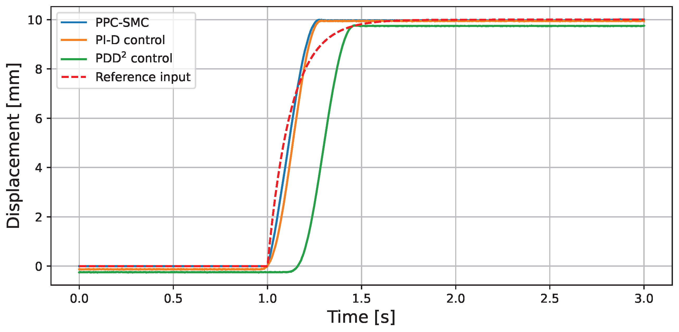
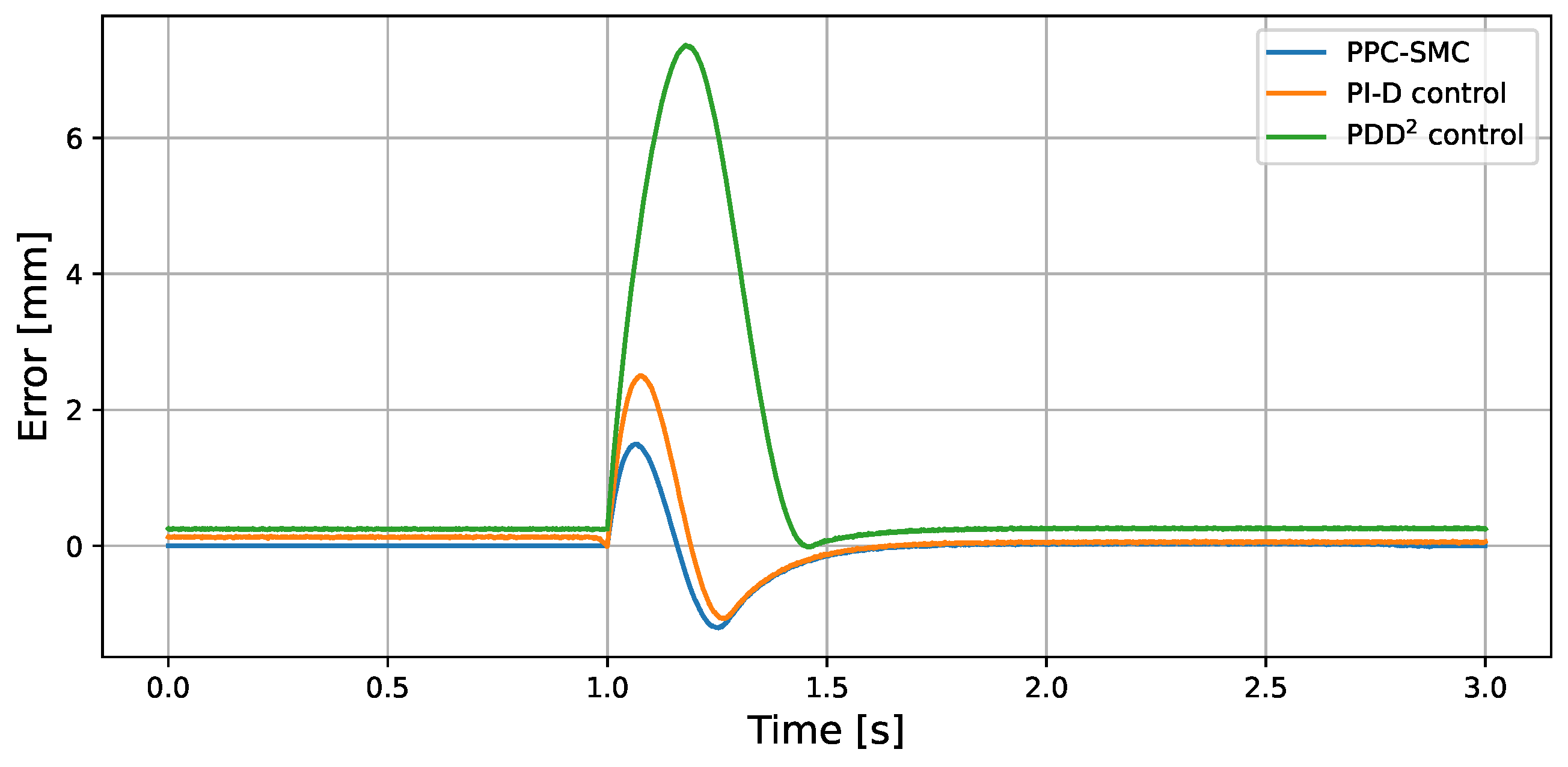
• By applying filtered right coprime factorization, the plant structure is simplified, allowing for the application of strict PPC-SMC to pneumatic stage systems with complex nonlinearities. This enables a more precise configuration of PPC-SMC that incorporates the nonlinearities of the pneumatic stage, resulting in a smaller performance function. Thus, the maximum error can be reduced compared to previous methods, contributing to even more precise positioning of the pneumatic stage.
• Experimental comparisons with previous studies were conducted, confirming that the proposed method achieves the smallest steady-state error.

The structure of this paper is as follows. First, Section 2 explains the control theory used in this study. Next, Section 3 describes the pneumatic stage utilized in this research and presents the problem setting. Then, Section 4 details the proposed control system. After that, Section 5 presents and discusses the experimental results. Finally, Section 6 concludes the paper.

2. Preparations

This section explains the filtered right coprime factorization and PPC-SMC.

2.1. Definition of Operator

In this study, an operator is defined as a “mapping” from an arbitrary input space to an output space [22,23]. This allows the nonlinear behavior of the controlled system to be expressed as a mapping that relates input and output signals. The notation $F:U\to Y$ used hereafter refers to a mapping by the operator F from the input signal space U to the output signal space Y. From this point forward, input and output signals are represented as time functions $u\left(t\right)\in U$ and $y\left(t\right)\in Y$, respectively, and the output over an arbitrary time interval is expressed as

$$\begin{array}{c}\hfill y\left(t\right)=F\left(u\right(t\left)\right).\end{array}$$

(1)

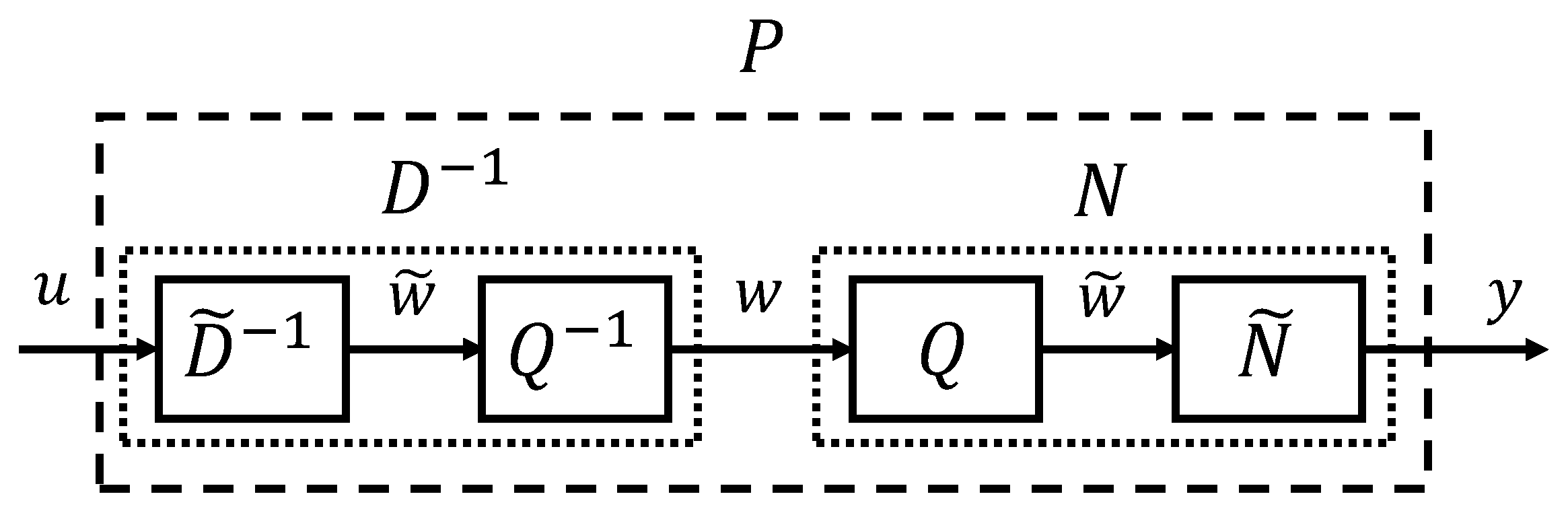
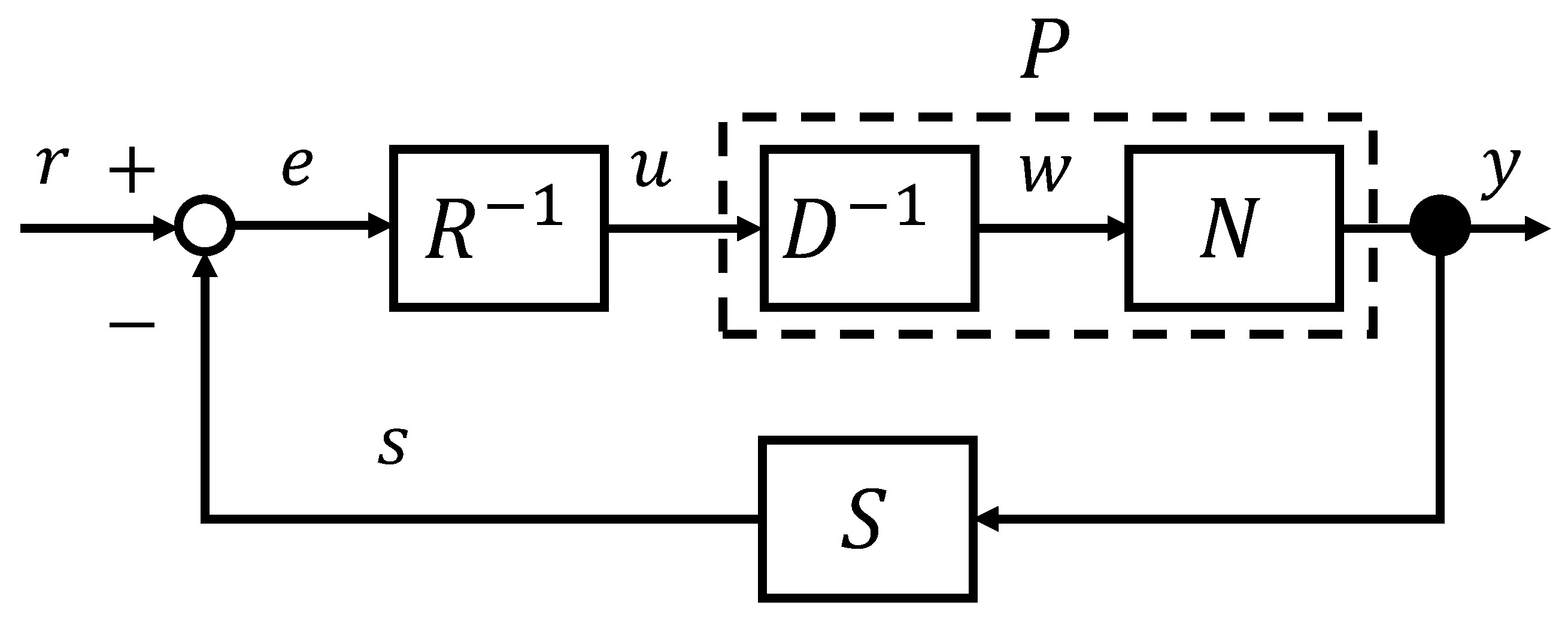
2.2. Filtered Right Comprime Factorization Based on Operator Theory

Let the input space, quasi-state space, and output space be denoted as U, W, and Y, respectively [22,23]. Consider a nonlinear plant represented by the operator $P:U\to Y$. Suppose there exist a stable operator $N:W\to Y$ and a stable and invertible operator $D:W\to U$ such that the nonlinear plant P can be expressed as

$$\begin{array}{c}\hfill P=N{D}^{-1},\end{array}$$

(2)

where the operators N and D represent the right factorization of P. Let $Q:W\to W$ be a stable and invertible operator with filtering characteristics [21]. Then, the operators $N:W\to Y$ and $D:W\to U$, defined as $N=\tilde{N}Q$ and $D=\tilde{D}Q$, also form a right factorization of P, as illustrated in Figure 1. By appropriately designing Q, noise mitigation can be effectively achieved [21]. Here, $u\left(t\right)\in U$ is the control input, $w\left(t\right)\in W$ is the quasi-state signal, and $y\left(t\right)\in Y$ is the output signal.

Furthermore, suppose there exist a stable operator $S:Y\to W$ and a stable and invertible operator $R:U\to W$ satisfying the following Bezout identity:

$$\begin{array}{c}\hfill SN+RD=M,\end{array}$$

(3)

where $M:W\to W$ is a unimodular operator, and N and D are the right coprime factorizations of P. The unimodular operator M refers to an operator that is stable and has a stable inverse. When Equation (3) holds, as shown in Figure 2, BIBO stability (Bounded-Input Bounded-Output stability) from the reference input $r\left(t\right)\in W$ to the output $y\left(t\right)$ is guaranteed. When the system is stabilized by right coprime factorization, the output $y\left(t\right)$ and reference input $r\left(t\right)$ can be expressed as

$$\begin{array}{cc}\hfill y\left(t\right)=& P\left(u\left(t\right)\right),\hfill \\ \hfill =& P\left(R^{-1}\left(r\left(t\right)-SN\left(w\left(t\right)\right)\right)\right),\hfill \\ \hfill =& P\left(R^{-1}\left(M\left(w\left(t\right)\right)-SN\left(w\left(t\right)\right)\right)\right),\hfill \\ \hfill =& PD\left(w\left(t\right)\right),\hfill \\ \hfill =& N\left(w\left(t\right)\right),\hfill \\ \hfill =& N{M}^{-1}\left(r\left(t\right)\right).\hfill \end{array}$$

(4)

Note that, according to the Bezout identity, the operator $D^{-1}$ is stabilized. Hereafter, we define the operator $P^{\prime }$ as $P^{\prime }=N{M}^{-1}$.

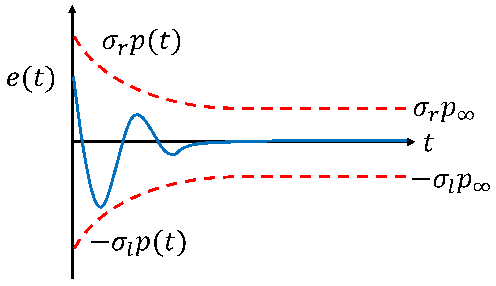
2.3. Prescribed Performance Control (PPC)

Before describing PPC-SMC, we explain PPC [24,25]. PPC is a control method that guarantees the error remains within the performance function $p\left(t\right)$, as illustrated in Figure 3. The performance function $p\left(t\right)$ is given by

$$\begin{array}{c}\hfill p\left(t\right)=(p_0-p_{\infty })e^{-\lambda t}+p_{\infty },\end{array}$$

(5)

where $p_0,p_{\infty },\lambda >0$ are the initial value, final value, and decay constant, respectively. Now consider a function such that the error $e\left(t\right)$ is constrained within the following range:

$$\begin{array}{c}\hfill -{\sigma }_{L}p\left(t\right)<e\left(t\right)<{\sigma }_{R}p\left(t\right),\end{array}$$

(6)

where $0<{\sigma }_L,{\sigma }_R<1$ are design parameters. Next, define the function $\Xi$ as

$$\begin{array}{c}\hfill {\displaystyle \frac{e\left(t\right)}{p\left(t\right)}}=\Xi \left(\tilde{e}\left(t\right)\right).\end{array}$$

(7)

By defining as in Equation (7), the error $e\left(t\right)$ containing the constraint information can be directly handled. To ensure $\tilde{e}\left(t\right)$ remains within the designed range, it is constructed as

$$\begin{array}{c}\hfill \Xi \left(\tilde{e}\left(t\right)\right)={\displaystyle \frac{{\sigma }_R{e}^{\tilde{e}\left(t\right)}-{\sigma }_L{e}^{-\tilde{e}\left(t\right)}}{e^{\tilde{e}\left(t\right)}+e^{-\tilde{e}\left(t\right)}}}.\end{array}$$

(8)

From Equations (7) and (8), $\tilde{e}\left(t\right)$ is given by

$$\begin{array}{c}\hfill \tilde{e}\left(t\right)={\Xi }^{-1}\left({\displaystyle \frac{e\left(t\right)}{p\left(t\right)}}\right)={\displaystyle \frac{1}{2}}\ln \left({\displaystyle \frac{e\left(t\right)/p\left(t\right)+{\sigma }_L}{{\sigma }_R-e\left(t\right)/p\left(t\right)}}\right).\end{array}$$

(9)

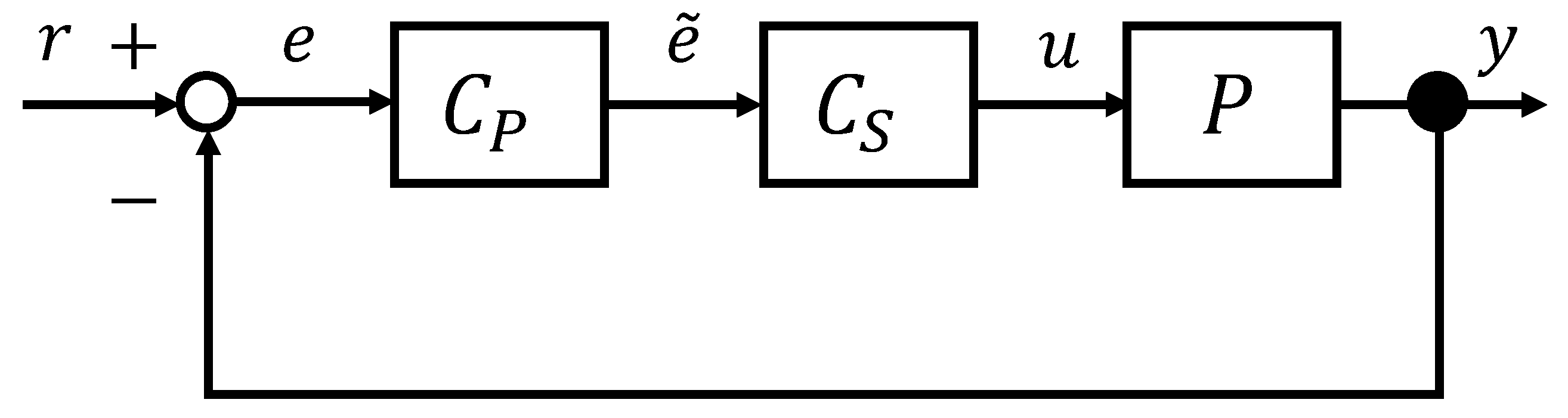
2.4. Prescribed Performance Control–Sliding Mode Control (PPC-SMC)

PPC-SMC is a method in which the switching surface is designed to include the output of PPC [26,27]. In Figure 4, the operator $C_P$ represents PPC, and the operator $C_S$ represents SMC. This enables safe control by ensuring that the error $e\left(t\right)$ does not exceed the desired range. The switching surface $\sigma \left(t\right)$ of PPC-SMC can be expressed, for example, as

$$\begin{array}{c}\hfill \sigma \left(t\right)={\displaystyle \frac{d}{dt}}{\Xi }^{-1}\left({\displaystyle \frac{e\left(t\right)}{p\left(t\right)}}\right)+K{\Xi }^{-1}\left({\displaystyle \frac{e\left(t\right)}{p\left(t\right)}}\right),\end{array}$$

(10)

where ${\Xi }^{-1}\left({\displaystyle \frac{e\left(t\right)}{p\left(t\right)}}\right)$ is defined in Equation (9).

3. Pneumatic Stage and Problem Setting

This section describes the overview of the pneumatic stage used in this study and the problem setting.

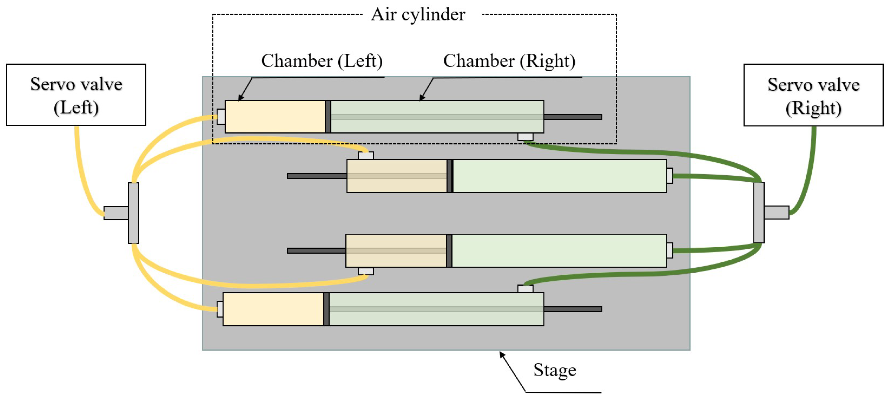
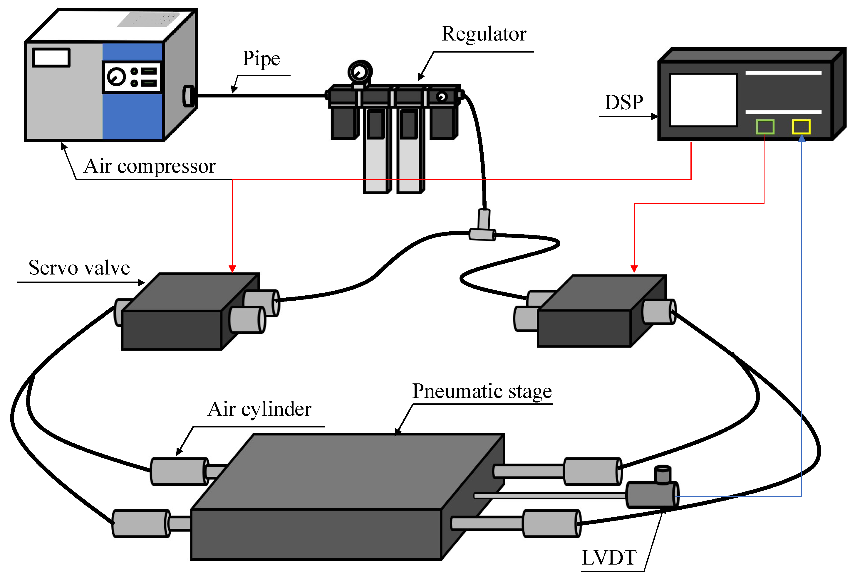
3.1. Pneumatic Stage

The pneumatic stage used in the experiment is shown in Figure 5, and an overview of its operation is illustrated in Figure 6. The stage, located at the upper left in the photograph, is supported by rolling bearings and moves along a straight line. As shown in Figure 6, four double-acting pneumatic cylinders are used for actuation. Pneumatic control is achieved using two pairs of servo valves located at the front of Figure 5, with each valve appropriately piped to the cylinder ports to generate thrust to the right or left. By supplying air pressure to the right servo valve, the stage moves to the left, and by supplying air pressure to the left servo valve, the stage moves to the right. The stage position is measured using a Linear Variable Differential Transformer (LVDT) placed on the right side of the stage. Next, the overall system configuration is explained in Figure 7. The pressure supplied to the servo valves is generated by a compressor, purified and depressurized by a regulator, and then delivered to the valves. Control computation is performed by a Digital Signal Processor (DSP). The DSP receives position information from the LVDT and outputs signals to control the opening and closing of the left and right servo valves. The servo valves are not controlled independently; the voltages $u_r$ and $u_l$ supplied to each valve are determined as differential signals from the control input u calculated by the controller as follows:

$$\begin{array}{cc}\hfill u_r& =u+u_0,\hfill \end{array}$$

(11)

$$\begin{array}{cc}\hfill u_l& =-u+u_0,\hfill \end{array}$$

(12)

where $u_0$ is the offset voltage of the valves and is set to $5.0\mathrm{V}$ in this equipment.

According to [20], the mathematical model of the pneumatic stage is given as

$$\begin{array}{c}\hfill P:\left\{\begin{array}{c}\ddot{y}\left(t\right)=-{\displaystyle \frac{F_r\left(\dot{y}\left(t\right)\right)}{m}}-{\displaystyle \frac{k}{m}}y\left(t\right)+{\displaystyle \frac{4S_d}{m}}p\left(t\right)\hfill \\ \dot{p}\left(t\right)=-{\displaystyle \frac{1}{T_{air}}}p\left(t\right)+{\displaystyle \frac{K_{air}}{T_{air}}}u\left(t\right)\hfill \\ F_r\left(t\right)={\sigma }_{0}z\left(t\right)+{\sigma }_1\dot{z}\left(t\right)+{\sigma }_2\left(\dot{y}\left(t\right)+T\ddot{y}\left(t\right)\right)\hfill \\ \dot{z}\left(t\right)=\dot{y}\left(t\right)-{\displaystyle \frac{{\sigma }_{0}z\left(t\right)}{g\left(\dot{y}\left(t\right),h_l\left(t\right)\right)}}\dot{y}\left(t\right)\hfill \\ g\left(\dot{y}\left(t\right),h_l\left(t\right)\right)=F_c+[\left(1-h_l\left(t\right)\right)F_s-F_c]e^{-{\left(\dot{y}\left(t\right)/v_s\right)}^n}\hfill \\ {\dot{h}}_l\left(t\right)={\displaystyle \frac{1}{{\tau }_h}}\left(h_{ss}\left(t\right)-h_l\left(t\right)\right)\hfill \\ {\tau }_h=\left\{\begin{array}{cc}\hfill {\tau }_{hp}& (v\left(t\right)\ne 0,h_l\left(t\right)\le h_{ss})\hfill \\ \hfill {\tau }_{hn}& (v\left(t\right)\ne 0,h_l\left(t\right)>h_{ss})\hfill \\ \hfill {\tau }_{h0}& \left(v\right(t)=0)\hfill \end{array}\right.\hfill \\ h_{ss}\left(t\right)=\left\{\begin{array}{cc}{K}_f{\left|v\left(t\right)\right|}^{2/3}\hfill & \hfill \left(\right|v\left(t\right)|\le |v_b\left|\right)\\ K_f{\left|v_b\right|}^{2/3}\hfill & \hfill \left(\right|v\left(t\right)|>|v_b\left|\right)\end{array}\right.\hfill \\ K_f=\left(1-{\displaystyle \frac{F_c}{F_s}}\right){\left|v_b\right|}^{-2/3}\hfill \end{array}\right.,\end{array}$$

(13)

where the LuGre model is used as the friction model. A description of each parameter is provided in

Table 1. Parameters of pneumatic stage.

Symbol	Description
z	Average deflection of sliding surface
${\sigma }_0$	Bristle stiffness
${\sigma }_1$	Microviscous friction coefficient
${\sigma }_2$	Coefficient of viscous friction
v	Relative velocity of piston and cylinder
$v_s$	Stribeck speed
$v_b$	Maximum speed of lubrication film thickness change
$h_l$	Non-dimensional non-stationary lubricant film thickness
$h_{ss}$	Non-dimensional steady-state lubricant film thickness
T	Time constants for fluid friction dynamics
$F_r$	Frictional force
$F_c$	Coulomb’s friction force
$F_s$	Maximum static friction
${\tau }_h$	Time constant of lubricant film dynamics
$K_f$	Proportionality constant of lubricant film thickness
m	Mass of stage
$S_d$	Piston cross-sectional area
k	Spring constant
$T_{air}$	Servo valve time constant
$K_{air}$	Servo valve gain

.

3.2. Problem Setting

Pneumatic stages contain many nonlinear elements such as friction and compressed air, and electrical noise can further degrade positioning accuracy [21].

In this study, we combine filtered right coprime factorization and PPC-SMC to achieve safe, fast, and high-precision position control of a pneumatic stage. The inner loop uses filtered right coprime factorization to guarantee stability, suppress electrical noise, and equivalently transform the system into a linear one, thereby facilitating the design of PPC-SMC. The outer loop employs PPC-SMC to constrain the tracking error within a user-defined range, enabling fast and robust control. Experimental results on the actual system demonstrate the effectiveness of the proposed control scheme in comparison with previous studies [19,20].

4. Control System Design

In this section, we design the control system. The overall control system is shown in Figure 8.

4.1. Filtered Right Coprime Factorization

The mathematical model of the pneumatic stage is given by Equation (13). However, for simplicity, some parts of Equation (13) are omitted in the following expressions. To remove noise, the operator Q is designed as a low-pass filter:

$$\begin{array}{c}\hfill Q\left(w\left(t\right)\right):\dot{\tilde{w}}\left(t\right)={\displaystyle \frac{1}{T_{LPF}}}(-\tilde{w}\left(t\right)+w\left(t\right)),\end{array}$$

(14)

where $T_{LPF}>0$ represents the time constant of the filter. At this time, the operators N and D are expressed as follows:

$$\begin{array}{cc}\hfill & N\left(w\left(t\right)\right):\left\{\begin{array}{c}{\dot{\tilde{w}}}_n\left(t\right)={\displaystyle \frac{1}{T_{LPF}}}(-{\tilde{w}}_n\left(t\right)+w\left(t\right))\hfill \\ {\ddot{x}}_n\left(t\right)=-{\displaystyle \frac{f_s}{m}}{\dot{x}}_n\left(t\right)-{\displaystyle \frac{k}{m}}{x}_n\left(t\right)+{\tilde{w}}_n\left(t\right)\hfill \\ y\left(t\right)=x_n\left(t\right)\hfill \end{array}\right.,\hfill \end{array}$$

(15)

$$\begin{array}{cc}\hfill & D\left(w\left(t\right)\right):\left\{\begin{array}{c}\begin{array}{c}{\dot{\tilde{w}}}_d\left(t\right)={\displaystyle \frac{1}{T_{LPF}}}(-{\tilde{w}}_d\left(t\right)+w\left(t\right))\hfill \\ {\ddot{x}}_{d2}\left(t\right)=-{\displaystyle \frac{f_s}{m}}{\dot{x}}_{d2}\left(t\right)-{\displaystyle \frac{k}{m}}{x}_{d2}\left(t\right)+{\tilde{w}}_d\left(t\right)\hfill \\ x_{d1}\left(t\right)=-{\displaystyle \frac{m}{4S_d}}{\ddot{x}}_{d2}\left(t\right)-{\displaystyle \frac{F_r\left({\dot{x}}_{d2}\left(t\right)\right)}{4S_d}}+{\displaystyle \frac{k}{4S_d}}{x}_{d2}\left(t\right)\hfill \\ u\left(t\right)=-{\displaystyle \frac{T_{air}}{K_{air}}}{\dot{x}}_{d1}\left(t\right)+{\displaystyle \frac{1}{K_{air}}}{x}_{d1}\left(t\right)\hfill \end{array}\end{array}\right.,\hfill \end{array}$$

(16)

where $f_s$ is the coefficient of the damper system modeled as a second-order lag system in previous research [19]. Next, the operators S, R, and M are designed to satisfy the Bezout identity (3). The operator S is designed as

$$\begin{array}{cc}\hfill & S\left(y\left(t\right)\right):s\left(t\right)=y\left(t\right).\hfill \end{array}$$

(17)

The unimodular operator M is designed as

$$\begin{array}{cc}\hfill & M\left(w\left(t\right)\right):r^{*}\left(t\right)={\displaystyle \frac{1}{g_d}}w\left(t\right),\hfill \end{array}$$

(18)

where $g_d>0$ is a design parameter. From the Bezout identity (3), the operator R is derived as

$$\begin{array}{cc}\hfill SN+RD& =M,\hfill \\ \hfill RD& =M-SN,\hfill \\ \hfill R& =\left(M-SN\right)D^{-1}.\hfill \end{array}$$

(19)

From Equations (15)–(19), the operator R can be expressed as

$$\begin{array}{cc}\hfill & R:\left\{\begin{array}{c}\begin{array}{c}{\dot{x}}_{rd1}\left(t\right)=-{\displaystyle \frac{1}{T_{air}}}{x}_{rd1}\left(t\right)+{\displaystyle \frac{K_{air}}{T_{air}}}u\left(t\right)\hfill \\ {\ddot{x}}_{rd2}\left(t\right)=-{\displaystyle \frac{F_r\left({\dot{x}}_{rd2}\left(t\right)\right)}{m}}-{\displaystyle \frac{k}{m}}{x}_{rd2}\left(t\right)+{\displaystyle \frac{4S_d}{m}}{x}_{rd1}\left(t\right)\hfill \\ {\tilde{w}}_{rd}\left(t\right)={\ddot{x}}_{rd2}\left(t\right)-{\displaystyle \frac{f_s}{m}}{\dot{x}}_{rd2}\left(t\right)+{\displaystyle \frac{k}{m}}{x}_{rd2}\left(t\right)\hfill \\ w_{rd}\left(t\right)=T_{LPF}{\dot{\tilde{w}}}_{rd}\left(t\right)+{\tilde{w}}_{rd}\left(t\right)\hfill \\ {\ddot{x}}_{rn}\left(t\right)=-{\displaystyle \frac{f_s}{m}}{x}_{rn}\left(t\right)-{\displaystyle \frac{k}{m}}{x}_{rn}\left(t\right)+{\tilde{w}}_{rd}\left(t\right)\hfill \\ x_m\left(t\right)={\displaystyle \frac{1}{g_d}}{w}_{rd}\left(t\right)\hfill \\ e^{*}\left(t\right)=x_m\left(t\right)-x_{rn}\left(t\right)\hfill \end{array}\end{array}\right..\hfill \end{array}$$

(20)

Thus, the stability from $r^{*}\left(t\right)$ to $y\left(t\right)$ is guaranteed. Therefore, the operator $P^{\prime }$ can be expressed as

$$\begin{array}{cc}\hfill & P^{\prime }:\left\{\begin{array}{cc}\hfill \dot{\tilde{w}}\left(t\right)& ={\displaystyle \frac{1}{T_{LPF}}}(-\tilde{w}\left(t\right)+g_d{r}^{*}\left(t\right))\hfill \\ \hfill \ddot{y}\left(t\right)& =-{\displaystyle \frac{f_s}{m}}\dot{y}\left(t\right)-{\displaystyle \frac{k}{m}}y\left(t\right)+\tilde{w}\left(t\right)\hfill \end{array}\right..\hfill \end{array}$$

(21)

4.2. PPC-SMC Controller

Based on Equation (21), we design the PPC-SMC controller. First, we simplify the notation of Equation (21) as

$$\begin{array}{cc}\hfill \ddot{y}\left(t\right)& =-{\displaystyle \frac{f_s}{m}}\dot{y}\left(t\right)-{\displaystyle \frac{k}{m}}y\left(t\right)+g_d(1-e^{-{\displaystyle \frac{t}{T_{LPF}}}})r^{*}\left(t\right),\hfill \\ \hfill & =-a_1\dot{y}\left(t\right)-a_{2}y\left(t\right)+f\left(t\right)r^{*}\left(t\right).\hfill \end{array}$$

(22)

Next, the operator $C_P$ is designed. The performance functions $p\left(t\right)$ and $\tilde{e}\left(t\right)$ are designed as

$$\begin{array}{c}\hfill \left\{\begin{array}{c}p\left(t\right)=(p_0-p_{\infty })e^{-\lambda t}+p_{\infty }\hfill \\ \tilde{e}\left(t\right)={\displaystyle \frac{1}{2}}\ln \left({\displaystyle \frac{e\left(t\right)/p\left(t\right)+{\sigma }_L}{{\sigma }_R-e\left(t\right)/p\left(t\right)}}\right)={\displaystyle \frac{1}{2}}\ln \left({\displaystyle \frac{h\left(t\right)+{\sigma }_L}{{\sigma }_R-h\left(t\right)}}\right)\hfill \end{array}\right.,\end{array}$$

(23)

where $h\left(t\right)=e\left(t\right)/p\left(t\right)$.

In addition, SMC is designed. Then, the switching surface $\sigma \left(t\right)$ is designed as

$$\begin{array}{c}\hfill \sigma \left(t\right)=\dot{\tilde{e}}\left(t\right)+K\tilde{e}\left(t\right),\end{array}$$

(24)

where $K>0$ is a design parameter. Then, the function $V\left(t\right)$ is defined as

$$\begin{array}{c}\hfill V\left(t\right)={\displaystyle \frac{1}{2}}{\sigma }^2\left(t\right).\end{array}$$

(25)

SMC is designed so that Equation (25) serves as a Lyapunov function. Then, Equation (25) can be expressed as

$$\begin{array}{cc}\hfill \dot{V}\left(t\right)& =\sigma \left(t\right)\dot{\sigma }\left(t\right),\hfill \\ \hfill & =\sigma \left(t\right)(\ddot{\tilde{e}}\left(t\right)+K\dot{\tilde{e}}\left(t\right)).\hfill \end{array}$$

(26)

At this time, $\dot{\tilde{e}}\left(t\right)$ and $\ddot{\tilde{e}}\left(t\right)$ are expressed as follows:

$$\begin{array}{cc}\hfill \dot{\tilde{e}}\left(t\right)=& {\displaystyle \frac{1}{2}}·{\displaystyle \frac{\dot{h}\left(t\right)({\sigma }_L+{\sigma }_R)}{\{h\left(t\right)+{\sigma }_L\}\{{\sigma }_R-h\left(t\right)\}}},\hfill \\ \hfill \ddot{\tilde{e}}\left(t\right)=& {\displaystyle \frac{1}{2}}·{\displaystyle \frac{\ddot{h}\left(t\right)({\sigma }_L+{\sigma }_R)\{h\left(t\right)+{\sigma }_L\}\{{\sigma }_R-h\left(t\right)\}+\{2h\left(t\right)\dot{h}\left(t\right)+({\sigma }_L-{\sigma }_R)\dot{h}\left(t\right)\}({\sigma }_L+{\sigma }_R)}{{\left[\{h\left(t\right)+{\sigma }_L\}\{{\sigma }_R-h\left(t\right)\}\right]}^2}},\hfill \end{array}$$

(27)

$$\begin{array}{cc}=\hfill & {\displaystyle \frac{1}{2{\left\{B\left(t\right)\right\}}^2}}\left\{\ddot{h}\left(t\right)A\left(t\right)+C\left(t\right)\right\},\hfill \end{array}$$

(28)

where $A\left(t\right)$, $B\left(t\right)$, and $C\left(t\right)$ are defined as

$$\begin{array}{c}\hfill \left\{\begin{array}{c}A\left(t\right)=({\sigma }_L+{\sigma }_R)\{h\left(t\right)+{\sigma }_L\}\{{\sigma }_R-h\left(t\right)\}\hfill \\ B\left(t\right)=\{h\left(t\right)+{\sigma }_L\}\{{\sigma }_R-h\left(t\right)\}\hfill \\ C\left(t\right)=\left\{2h\left(t\right)\dot{h}\left(t\right)+({\sigma }_L-{\sigma }_R)\dot{h}\left(t\right)\right\}({\sigma }_L+{\sigma }_R)\hfill \end{array}\right..\end{array}$$

(29)

In addition, $\dot{h}\left(t\right)$ and $\ddot{h}\left(t\right)$ are given by

$$\begin{array}{c}\hfill \left\{\begin{array}{c}\dot{h}\left(t\right)={\displaystyle \frac{\dot{e}\left(t\right)p\left(t\right)-e\left(t\right)\dot{p}\left(t\right)}{{\left\{p\left(t\right)\right\}}^2}}\hfill \\ \ddot{h}\left(t\right)={\displaystyle \frac{\ddot{e}\left(t\right)}{p\left(t\right)}}+{\displaystyle \frac{2e\left(t\right){\left\{\dot{p}\left(t\right)\right\}}^2-e\left(t\right)p\left(t\right)\ddot{p}\left(t\right)-2\dot{e}\left(t\right)p\left(t\right)\dot{p}\left(t\right)}{{\left\{p\left(t\right)\right\}}^2}}\hfill \\ ={\displaystyle \frac{\ddot{e}\left(t\right)}{p\left(t\right)}}+D\left(t\right)\hfill \end{array}\right.,\end{array}$$

(30)

where $D\left(t\right)$ is defined as

$$\begin{array}{c}\hfill D\left(t\right)={\displaystyle \frac{2e\left(t\right){\left\{\dot{p}\left(t\right)\right\}}^2-e\left(t\right)p\left(t\right)\ddot{p}\left(t\right)-2\dot{e}\left(t\right)p\left(t\right)\dot{p}\left(t\right)}{{\left\{p\left(t\right)\right\}}^2}}.\end{array}$$

(31)

From Equations (27)–(31), Equation (26) can be expressed as

$$\begin{array}{cc}\hfill \dot{V}\left(t\right)& =\sigma \left(t\right)\dot{\sigma }\left(t\right),\hfill \\ \hfill & =\sigma \left(t\right)(\ddot{\tilde{e}}\left(t\right)+K\tilde{e}\left(t\right)),\hfill \\ \hfill & =\sigma \left(t\right)\left[{\displaystyle \frac{1}{2{\left\{B\left(t\right)\right\}}^2}}\{\ddot{h}\left(t\right)A\left(t\right)+C\left(t\right)\}+K\dot{\tilde{e}}\left(t\right)\right],\hfill \\ \hfill & =\sigma \left(t\right)\left[{\displaystyle \frac{1}{2{\left\{B\left(t\right)\right\}}^2}}\left\{\left({\displaystyle \frac{\ddot{e}\left(t\right)}{p\left(t\right)}}+D\left(t\right)\right)A\left(t\right)+C\left(t\right)\right\}+K\dot{\tilde{e}}\left(t\right)\right],\hfill \\ \hfill & =\sigma \left(t\right)\left\{{\displaystyle \frac{A\left(t\right)}{2{\left\{B\left(t\right)\right\}}^{2}p\left(t\right)}}\ddot{e}\left(t\right)+{\displaystyle \frac{A\left(t\right)D\left(t\right)}{2{\left\{B\left(t\right)\right\}}^2}}+{\displaystyle \frac{C\left(t\right)}{2{\left\{B\left(t\right)\right\}}^2+K\dot{\tilde{e}}\left(t\right)}}\right\},\hfill \\ \hfill & =\sigma \left(t\right)\left\{\tilde{A}\left(t\right)\ddot{e}\left(t\right)+\tilde{E}\left(t\right)+K\dot{\tilde{e}}\left(t\right)\right\},\hfill \end{array}$$

(32)

where the variables $\tilde{A},\tilde{E}$ are defined as

$$\begin{array}{c}\hfill \left\{\begin{array}{c}\tilde{A}\left(t\right)={\displaystyle \frac{A\left(t\right)}{2{\left\{B\left(t\right)\right\}}^{2}p\left(t\right)}}\hfill \\ \tilde{E}\left(t\right)={\displaystyle \frac{A\left(t\right)D\left(t\right)}{2{\left\{B\left(t\right)\right\}}^2}}+{\displaystyle \frac{C\left(t\right)}{2{\left\{B\left(t\right)\right\}}^2}}\hfill \end{array}\right..\end{array}$$

(33)

From Equation (32), we define $r^{*}\left(t\right)=r_1^{*}\left(t\right)+r_2^{*}\left(t\right)+r_3^{*}\left(t\right)+r_4^{*}\left(t\right)+r_5^{*}\left(t\right)$, and then

$$\begin{array}{cc}\hfill \dot{V}\left(t\right)=& \sigma \left(t\right)\left\{\tilde{A}\left(t\right)\ddot{e}\left(t\right)+\tilde{E}\left(t\right)+K\dot{\tilde{e}}\left(t\right)\right\},\hfill \\ \hfill =& \sigma \left(t\right)\left[\tilde{A}\left(t\right)\{\ddot{r}\left(t\right)-\ddot{y}\left(t\right)\}+\tilde{E}\left(t\right)+K\dot{\tilde{e}}\left(t\right)\right],\hfill \\ \hfill =& \sigma \left(t\right)\tilde{A}\left(t\right)\ddot{r}\left(t\right)+\sigma \left(t\right)\tilde{A}\left(t\right)a_1\dot{y}\left(t\right)+\sigma \left(t\right)\tilde{A}\left(t\right)a_{2}y\left(t\right)+\sigma \left(t\right)\tilde{E}\left(t\right)+\sigma \left(t\right)K\tilde{e}\left(t\right)\hfill \\ \hfill & -\sigma \left(t\right)\tilde{A}\left(t\right)f\left(t\right)r^{*}\left(t\right),\hfill \\ \hfill =& \{\sigma \left(t\right)\tilde{A}\left(t\right)\ddot{r}\left(t\right)-\sigma \left(t\right)\tilde{A}\left(t\right)f\left(t\right)r_1^{*}\left(t\right)\}+\{\sigma \left(t\right)\tilde{A}\left(t\right)a_1\dot{y}\left(t\right)-\sigma \left(t\right)\tilde{A}\left(t\right)f\left(t\right)r_2^{*}\left(t\right)\}\hfill \\ \hfill & +\{\sigma \left(t\right)\tilde{A}\left(t\right)a_{2}y\left(t\right)-\sigma \left(t\right)\tilde{A}\left(t\right)f\left(t\right)r_3^{*}\left(t\right)\}+\{\sigma \left(t\right)\tilde{E}\left(t\right)-\sigma \left(t\right)\tilde{A}\left(t\right)f\left(t\right)r_4^{*}\left(t\right)\}\hfill \\ \hfill & +\{\sigma \left(t\right)K\dot{\tilde{e}}\left(t\right)-\sigma \left(t\right)\tilde{A}\left(t\right)f\left(t\right)r_5^{*}\left(t\right)\}.\hfill \end{array}$$

(34)

We can transform it as shown in Equation (34). Therefore, we design each $r_i^{*}\left(t\right)(i=1,\dots ,5)$ such that each term within the curly brackets is less than zero. Each term is designed as follows:

$$\begin{array}{cc}\hfill & r_1^{*}\left(t\right)=\mathrm{sgn}\left(\sigma \left(t\right)\right){\displaystyle \frac{\tilde{\ddot{r}}}{g_s}},\hfill \end{array}$$

(35)

$$\begin{array}{cc}\hfill & r_2^{*}\left(t\right)=\mathrm{sgn}\left(\sigma \left(t\right)\right){\displaystyle \frac{a_1}{g_s}}\left|\dot{y}\left(t\right)\right|,\hfill \end{array}$$

(36)

$$\begin{array}{cc}\hfill & r_3^{*}\left(t\right)=\mathrm{sgn}\left(\sigma \left(t\right)\right){\displaystyle \frac{a_2}{g_s}}\left|y\left(t\right)\right|,\hfill \end{array}$$

(37)

$$\begin{array}{cc}\hfill & r_4^{*}\left(t\right)={\displaystyle \frac{\mathrm{sgn}\left(\sigma \left(t\right)\right)}{g_s}}+{\displaystyle \frac{\tilde{E}\left(t\right)}{\tilde{A}\left(t\right)f\left(t\right)}},\hfill \end{array}$$

(38)

$$\begin{array}{cc}\hfill & r_5^{*}\left(t\right)=\mathrm{sgn}\left(\sigma \left(t\right)\right){\displaystyle \frac{K}{g_s\tilde{A}\left(t\right)}}|\dot{\tilde{e}}\left(t\right)|,\hfill \end{array}$$

(39)

where $g_s,\tilde{\ddot{r}}$ are design parameters that satisfy $0<g_s<f\left(t\right)(t\ge 0),\tilde{\ddot{r}}\ne 0,\tilde{\ddot{r}}>\left|\ddot{r}\left(t\right)\right|(t\ge 0)$, and sgn is the sign function. The derivations of Equations (35)–(39) are shown in Appendix A.

The control input designed according to this guideline becomes Equation (40):

$$\begin{array}{cc}\hfill r^{*}\left(t\right)=& {\displaystyle \frac{\mathrm{sat}\left(\sigma \left(t\right)\right)}{g_s}}\left(\ddot{r}\left(t\right)+a_1|\dot{y}\left(t\right)|+a_2|y\left(t\right)|+1+{\displaystyle \frac{K}{\tilde{A}\left(t\right)}}|\dot{\tilde{e}}\left(t\right)|\right)+{\displaystyle \frac{\tilde{E}\left(t\right)}{\tilde{A}\left(t\right)f\left(t\right)}},\hfill \end{array}$$

(40)

where $g_s>0$ is a design parameter,. To suppress chattering, the sign function sgn is approximated by the saturation function sat shown below:

$$\begin{array}{c}\hfill \mathrm{sat}\left(x\right)=\left\{\begin{array}{cc}1\hfill & (x>1)\hfill \\ x\hfill & (-1\le x\le 1)\hfill \\ -1\hfill & (x<-1)\hfill \end{array}\right.\end{array}$$

(41)

5. Experimental Results

In this section, based on the control system designed in Section 4, experiments of pneumatic stage position control are conducted to verify the effectiveness of the proposed method. The parameters for the LuGre model, the pneumatic stage, and the PPC-SMC controller are summarized in

Table 2. Experimental parameters.

Symbol	Value	Unit	Symbol	Value	Unit
${\sigma }_0$	$1.5\times {10}^4$	$\mathrm{N}/\mathrm{m}$	m	15	$\mathrm{kg}$
${\sigma }_1$	$0.01$	$\mathrm{N}·\mathrm{s}/\mathrm{m}$	$S_d$	198	${\mathrm{mm}}^2$
${\sigma }_2$	174	$\mathrm{N}·\mathrm{s}/\mathrm{m}$	k	$0.01$	$\mathrm{N}/\mathrm{m}$
$v_s$	$0.01$	$\mathrm{m}/\mathrm{s}$	$T_{air}$	$0.08$	$\mathrm{s}$
$v_b$	$0.005$	$\mathrm{m}/\mathrm{s}$	$K_{air}$	$4.2\times {10}^4$	$\mathrm{Pa}/\mathrm{V}$
T	0	$\mathrm{s}$	$g_d$	100	−
n	$0.5$	-	K	20	−
$F_c$	$0.4$	$\mathrm{N}$	f	218	$\mathrm{N}·\mathrm{s}/\mathrm{m}$
$F_s$	$0.41$	$\mathrm{N}$	$g_s$	99	−
${\tau }_{hp}$	$0.01$	$\mathrm{s}$	$b_0$	$0.6$	−
${\tau }_{hn}$	$0.2$	$\mathrm{s}$	$\tilde{\ddot{r}}$	5	−
${\tau }_{h0}$	20	$\mathrm{s}$	$h_d$	100	−
$T_{LPF}$	$0.01$	$\mathrm{s}$	$\lambda$	1	−
${\sigma }_L$	$0.6$	−	${\sigma }_R$	$0.6$	−
$p_0$	$0.02$	$\mathrm{m}$	$p_{\infty }$	$0.01$	$\mathrm{m}$

.

The experiment is conducted for 3 s with a sampling period of 0.1 ms, and the reference input $r\left(t\right)$ is applied at $t\ge 1$. Experiments are performed to compare the proposed method with previous studies [19,20]. The results when a step signal is applied to each method are shown in Figure 9 and Figure 10.

Table 3. Experimental result comparison.

Method	Settling Time	Steady-State Error	MAE	ITAE
PPC-SMC	$0.27\mathrm{s}$	$2\mathsf{\mu }\mathrm{m}$	$61\mathsf{\mu }\mathrm{m}$	$380\mathrm{mm}·\mathrm{s}$
PI-D control	$0.30\mathrm{s}$	$40\mathsf{\mu }\mathrm{m}$	$223\mathsf{\mu }\mathrm{m}$	$782\mathrm{mm}·\mathrm{s}$
PDD2 control	$0.47\mathrm{s}$	$200\mathsf{\mu }\mathrm{m}$	$822\mathsf{\mu }\mathrm{m}$	$3167\mathrm{mm}·\mathrm{s}$

presents the quantitative evaluation of the experiments. The settling time evaluates the time required for the output to reach a steady value, and the steady-state error is used to assess the difference between the output and the reference input after settling. Furthermore, the mean absolute error (MAE) evaluates the transient response error, while the integral of time-weighted absolute error (ITAE) is used to assess the steady-state response error separately from the steady-state error.

From Figure 9 and Figure 10, it can be seen that the proposed method achieves a faster response and smaller deviation. Furthermore, Table 3 shows that our proposed method outperforms the others in all evaluation metrics. The reason for this improvement is that the previous study [19] approximated the system as it as a mass–spring–damper model using frequency-domain approximation. In contrast, our study uses operator theory in the time domain to transform the system into a mass–spring–damper model, allowing us to handle the model in real time without approximation. Furthermore, compared to the previous study [20], our results are very similar. This is because both approaches employ operator theory in the time domain. The response time is almost the same in both cases, but our method shows superior steady-state error performance. This improvement is attributed to the fact that the previous study [20] used PI-D for trajectory tracking, whereas our study employs PPC-SMC.

6. Conclusions

In this paper, we proposed a control method that combines filtered right coprime factorization and PPC-SMC to achieve precise position control of a pneumatic stage. By integrating these two approaches, we achieved safe, robust, fast, and high-precision control. Experimental results demonstrated that the proposed method significantly reduced the settling time and greatly improved accuracy compared to previous studies. In future work, we plan to investigate methods for online optimization of controller parameters to further enhance control performance.

References

1. Bohr, M. A 30 year retrospective on Dennard’s MOSFET scaling paper. IEEE Solid-State Circuits Soc. Newsl. 2009, 12, 11–13. [Google Scholar] [CrossRef]
2. Wang, H.; Li, Q.; Zhou, F.; Zhang, J. High-Precision Positioning Stage Control Based on a Modified Disturbance Observer. Sensors 2024, 24, 591. [Google Scholar] [CrossRef] [PubMed]
3. Kawashima, K.; Arai, T.; Tadano, K.; Fujita, T.; Kagawa, T. Development of coarse/fine dual stage using pneumatically driven bellows actuator and cylinder with air bearings. Precis. Eng. 2010, 34, 526–533. [Google Scholar] [CrossRef]
4. Sato, K.; Sano, Y. Practical and intuitive controller design method for precision positioning of a pneumatic cylinder actuator stage. Precis. Eng. 2014, 38, 703–710. [Google Scholar] [CrossRef]
5. De Wit, C.C.; Olsson, H.; Åstrom, K.J.; Lischinsky, P. A new model for control of systems with friction. IEEE Trans. Autom. Control 1995, 40, 419–425. [Google Scholar] [CrossRef]
6. Yanada, H.; Sekikawa, Y. Modeling of dynamic behaviors of friction. Mechatronics 2008, 18, 330–339. [Google Scholar] [CrossRef]
7. Tran, X.B.; Hafizah, N.; Yanada, H. Modeling of dynamic friction behaviors of hydraulic cylinders. Mechatronics 2012, 22, 65–75. [Google Scholar] [CrossRef]
8. Xi, T.; Fujita, T.; Kehne, S.; Ikeda, R.; Fey, M.; Brecher, C. An extended LuGre model for estimating nonlinear frictions in feed drive systems of machine tools. Procedia CIRP 2022, 107, 452–457. [Google Scholar] [CrossRef]
9. Johanastrom, K.; Canudas-De-Wit, C. Revisiting the LuGre friction model. IEEE Control Syst. Mag. 2008, 28, 101–114. [Google Scholar] [CrossRef]
10. Freidovich, L.; Robertsson, A.; Shiriaev, A.; Johansson, R. LuGre-model-based friction compensation. IEEE Trans. Control Syst. Technol. 2009, 18, 194–200. [Google Scholar] [CrossRef]
11. Tran, X.B.; Yanada, H. Dynamic friction behaviors of pneumatic cylinders. Intell. Control Autom. 2013, 4, 180–190. [Google Scholar] [CrossRef]
12. Tran, X.B.; Dao, H.; Tran, K. A new mathematical model of friction for pneumatic cylinders. Proc. Inst. Mech. Eng. Part C J. Mech. Eng. Sci. 2016, 230, 2399–2412. [Google Scholar] [CrossRef]
13. Hildebrandt, A.; Neumann, R.; Sawodny, O. Optimal system design of siso-servopneumatic positioning drives. IEEE Trans. Control Syst. Technol. 2009, 18, 35–44. [Google Scholar] [CrossRef]
14. Zhao, L.; Yang, Y.; Xia, Y.; Liu, Z. Active disturbance rejection position control for a magnetic rodless pneumatic cylinder. IEEE Trans. Ind. Electron. 2015, 62, 5838–5846. [Google Scholar] [CrossRef]
15. Saravanakumar, D.; Mohan, B.; Muthuramalingam, T. A review on recent research trends in servo pneumatic positioning systems. Precis. Eng. 2017, 49, 481–492. [Google Scholar] [CrossRef]
16. Richer, E.; Hurmuzlu, Y. A high performance pneumatic force actuator system: Part I Nonlinear mathematical model. J. Dyn. Sys., Meas. Control 2000, 122, 416–425. [Google Scholar] [CrossRef]
17. Richer, E.; Hurmuzlu, Y. A high performance pneumatic force actuator system: Part II nonlinear controller design. J. Dyn. Sys. Meas. Control 2000, 122, 426–434. [Google Scholar] [CrossRef]
18. Ishii, H.; Wakui, S. Performance improvement of PDD 2 compensator embedded in position control for pneumatic stage. In Proceedings of the 2019 International Conference on Advanced Mechatronic Systems, Kusatsu, Japan, 26–28 August 2019; pp. 158–162. [Google Scholar]
19. Ishii, H.; Wakui, S. Proposal of Speeding up Scheme for Pneumatic Stage. In Proceedings of the 2019 IEEE International Conference on Mechatronics, Ilmenau, Germany, 18–20 March 2019; Volume 1, pp. 79–84. [Google Scholar]
20. Aoki, S.; Deng, M. Nonlinear position control of pneumatically driven stage considering friction characteristics of pneumatic cylinder. In Proceedings of the 2023 International Conference on Advanced Mechatronic Systems (ICAMechS), Melbourne, Australia, 4–7 September 2023; pp. 1–6. [Google Scholar] [CrossRef]
21. Tanabata, Y.; Deng, M. Filtered Right Coprime Factorization and Its Application to Control a Pneumatic Cylinder. Processes 2024, 12, 1475. [Google Scholar] [CrossRef]
22. De Figueiredo, R.J.; Chen, G. Nonlinear Feedback Control Systems: An Operator Theory Approach; Academic Press Professional, Inc.: Cambridge, MA, USA, 1993. [Google Scholar]
23. Deng, M. Operator-Based Nonlinear Control Systems: Design and Applications; John Wiley & Sons: Hoboken, NJ, USA, 2014. [Google Scholar]
24. Bechlioulis, C.P.; Rovithakis, G.A. Prescribed performance adaptive control of SISO feedback linearizable systems with disturbances. In Proceedings of the 2008 16th Mediterranean Conference on Control and Automation, Ajaccio, France, 25–27 June 2008; pp. 1035–1040. [Google Scholar] [CrossRef]
25. Bu, X. Prescribed performance control approaches, applications and challenges: A comprehensive survey. Asian J. Control 2021, 2020, 1–24. [Google Scholar] [CrossRef]
26. Yao, Y.; Zhuang, Y.; Xie, Y.; Xu, P.; Wu, C. Prescribed Performance Global Non-Singular Fast Terminal Sliding Mode Control of PMSM Based on Linear Extended State Observer. Actuators 2025, 14, 65. [Google Scholar] [CrossRef]
27. Nguyen, V.C.; Kim, S.H. A novel fixed-time prescribed performance sliding mode control for uncertain wheeled mobile robots. Sci. Rep. 2025, 15, 5340. [Google Scholar] [CrossRef]
Figure 1. Filtered right factorization.
Axioms 14 00534 g001
Figure 2. Feedback control system based on filtered right coprime factorization.
Axioms 14 00534 g002
Figure 3. Conceptual diagram of PPC.
Axioms 14 00534 g003
Figure 4. Overview diagram of PPC-SMC.
Axioms 14 00534 g004
Figure 5. Experimental setup.
Axioms 14 00534 g005
Figure 6. Schematic diagram of the experimental setup.
Axioms 14 00534 g006
Figure 7. Conceptual diagram of the experimental setup.
Axioms 14 00534 g007
Figure 8. Feedback control system based on filtered right coprime factorization and PPC-SMC.
Axioms 14 00534 g008
Figure 9. Displacement.
Axioms 14 00534 g009
Figure 10. Displacement error.
Axioms 14 00534 g010