Clifford Distributions Revisited

Abstract

In the framework of harmonic and Clifford analysis, specific distributions in Euclidean space of arbitrary dimension, which are of particular importance for theoretical physics, are once more thoroughly studied. Indeed, actions involving spherical coordinates, such as the radial derivative and multiplication and division by the radial distance, only make sense when considering so-called signumdistributions, that is, bounded linear functionals on a space of test functions showing a singularity at the origin. Introducing these signumdistributions, the actions of a whole series of scalar and vectorial differential operators on the distributions under consideration, lead to a number of surprising results, as illustrated by some examples in three-dimensional mathematical physics.

1. Introduction

The central notion in this paper is that of a distribution in Euclidean space ${\mathbb{R}}^m$. Let $\mathcal{D}\left({\mathbb{R}}^m\right)$ be the space of scalar-valued, infinitely differentiable functions $\phi :{\mathbb{R}}^m⟶\mathbb{R}or\mathbb{C}$, with compact support $supp\left[\phi \right]\subset {\mathbb{R}}^m$. This space $\mathcal{D}\left({\mathbb{R}}^m\right)$ is called a space of test functions. When equipped with an appropriate topology, its dual-space ${\mathcal{D}}^{\prime }\left({\mathbb{R}}^m\right)$ of continuous linear functionals is the space of standard distributions in ${\mathbb{R}}^m$. Some basic definitions and properties in distribution theory may be found in Appendix A.

In a series of papers, see [1] and the references therein, several families of distributions in Euclidean space ${\mathbb{R}}^m$ were thoroughly studied in the context of the theory of so-called monogenic functions, and this function theory is also termed Clifford analysis. This function theory is a direct and elegant generalization to higher dimensions of the theory of holomorphic functions in the complex plane and a refinement of harmonic analysis. We refer to Appendix E for the basic definitions in Clifford analysis.

Of particular importance to theoretical physics are the distribution families $T_{\lambda }$ and $U_{\lambda }$, $\lambda \in \mathbb{C}$ involving powers of the radial distance. They are defined using spherical coordinates through the following: $\underline{x}=r\underline{\omega },r=\left|\underline{x}\right|,\underline{\omega }={\displaystyle \frac{\underline{x}}{r}}={\displaystyle \frac{\underline{x}}{|\underline{x}|}}\in S^{m-1}$; therein, $S^{m-1}$ is the unit sphere in ${\mathbb{R}}^m$. In Section 3, we will illustrate the use of the spherical coordinates system in the lower-dimensional cases when $m=2$ and $m=3$.

Definition 1.

For all $\lambda \in \mathbb{C}$ and test functions $\phi \left(\underline{x}\right)\in \mathcal{D}\left({\mathbb{R}}^m\right)$, the distributions $T_{\lambda }$ and $U_{\lambda }$ are defined by

$$\langle T_{\lambda },\phi \left(\underline{x}\right)\rangle :=a_m\langle \mathrm{Fp}{r}_{+}^{\lambda +m-1},{\Sigma }^{\left(0\right)}\left[\phi \right]\left(r\right)\rangle$$

and

$$\langle U_{\lambda },\phi \left(\underline{x}\right)\rangle :=a_m\langle \mathrm{Fp}{r}_{+}^{\lambda +m-1},{\Sigma }^{\left(1\right)}\left[\phi \right]\left(r\right)\rangle ,$$

where the spherical means ${\Sigma }^{\left(0\right)}\left[\phi \right]$ and ${\Sigma }^{\left(1\right)}\left[\phi \right]$ are given by

$${\Sigma }^{\left(0\right)}\left[\phi \right]\left(r\right)={\displaystyle \frac{1}{a_m}}{\int }_{S^{m-1}}\phantom{\underline{\omega }}\phi \left(r\underline{\omega }\right)dS\left(\underline{\omega }\right)$$

and

$${\Sigma }^{\left(1\right)}\left[\phi \right]\left(r\right)={\displaystyle \frac{1}{a_m}}{\int }_{S^{m-1}}\underline{\omega }\phi \left(r\underline{\omega }\right)dS\left(\underline{\omega }\right),$$

where $a_m={\displaystyle \frac{2{\pi }^{m/2}}{\mathrm{\Gamma }(m/2)}}$ is the area of the unit sphere $S^{m-1}$, and Fp$r_{+}^{\mu },\mu \in \mathbb{C}$ represents the finite part distribution on the one-dimensional r-axis.

For the sake of completeness, we have included appendices with further information on the concept of distribution and the one-dimensional Finite Part distribution (see Appendix A), on distributions $T_{\lambda }$ and $U_{\lambda }$ (see Appendix B), and on spherical means (see Appendix C). We have also included an appendix, Appendix D, giving an overview of the properties of the most important distributions in both families.

Despite the fact that the distributions $T_{\lambda }$ are spherical in nature and that a formula such as ${\partial }_r{T}_{\lambda }=\lambda T_{\lambda -1}$ seems to be trivial, at the time the abovementioned papers were written, their radial derivative ${\partial }_r{T}_{\lambda }$ value was not yet studied. Meanwhile, it has become clear that the derivation of a distribution with respect to spherical coordinates is far from trivial. To put it straight, the radial derivative of a distribution cannot be a distribution. In his famous and seminal book [2], Laurent Schwartz writes on page 51: Using coordinate systems other than the Cartesian ones should be done with utmost care [our translation]. As an illustration, consider the delta distribution $\delta \left(\underline{x}\right)$: It is pointly supported at the origin. It is rotation-invariant: $\delta \left(A\underline{x}\right)=\delta \left(\underline{x}\right),\forall A\in \mathrm{SO}\left(m\right)$. It is even: $\delta (-\underline{x})=\delta \left(\underline{x}\right)$, and it is homogeneous of degree $(-m)$, where $\delta \left(a\underline{x}\right)={\displaystyle \frac{1}{{\left|a\right|}^m}}\delta \left(\underline{x}\right)$. Therefore, in an initial, naive, approach, one could think of its radial derivative ${\partial }_r\delta \left(\underline{x}\right)$ as being a distribution that remains pointly supported at the origin, rotation-invariant, even, and homogeneous of degree $(-m-1)$. Temporarily leaving aside the even character, based on the other cited characteristics, the distribution ${\partial }_r\delta \left(\underline{x}\right)$ should take the form

$${\partial }_r\delta \left(\underline{x}\right)=c_0{\partial }_{x_1}\delta \left(\underline{x}\right)+\dots +c_m{\partial }_{x_m}\delta \left(\underline{x}\right).$$

It becomes clear that such an approach to the radial derivation of the delta distribution is impossible because all distributions appearing in the sum on the right-hand side are odd and not rotation-invariant, whereas ${\partial }_r\delta \left(\underline{x}\right)$ is assumed to be even and rotation-invariant. It could be that ${\partial }_r\delta \left(\underline{x}\right)$ is either the zero distribution or is no longer pointly supported at the origin, but both of these possibilities are unacceptable.

In ref. [3], the problem of defining the radial derivative ${\partial }_r\delta \left(\underline{x}\right)$ of the delta distribution was solved by introducing a new concept, similar to but fundamentally different from a distribution, which was termed a signumdistribution. A signumdistribution is a continuous linear functional acting on a space of test functions that are smooth in ${\mathbb{R}}^m\setminus \left\{O\right\}$ and show a non-removable singularity at the origin. The definition and first properties of the signumdistributions are discussed in Section 2. It turns out that the radial derivative of the delta distribution is indeed a signumdistribution. Since the delta function is a fundamental mathematical modeling tool in a broad spectrum of theoretical physics and engineering sciences, we meanwhile undertook the enterprise of compiling a compendium [4] of interesting ready-to-use identities involving the delta distribution and the delta signumdistribution in higher-dimensional Euclidean space.

Actions on general distributions involving spherical coordinates were thoroughly studied in [5]. For a distribution $T\in {\mathcal{D}}^{\prime }\left({\mathbb{R}}^m\right)$, its radial derivative ${\partial }_{r}T$ is well defined, but not uniquely defined, as an equivalence class of signumdistributions. To make the paper self-contained, the main results about spherical actions on (signum)distributions are recalled in Section 2, Section 3, Section 4 and Section 5. In Section 6, we state the sufficient conditions under which the actions of a number of operators involving division by $\underline{x}$ or r are uniquely determined. In Section 8, we show a.o. that the radial derivative of the distributions $T_{\lambda }$ and $U_{\lambda }$ is uniquely defined as a signumdistribution belonging to two families of signumdistributions ${}^{s}T_{\lambda }$ and ${}^{s}U_{\lambda }$ which are closely related to the initial distribution families $T_{\lambda }$ and $U_{\lambda }$. In addition, other actions on the distributions $T_{\lambda }$ and $U_{\lambda }$ involving spherical coordinates are explored. In Section 7 and Section 9, special attention is paid to the Cartesian derivatives of signumdistributions in general and of the signumdistributions ${}^{s}T_{\lambda }$ and ${}^{s}U_{\lambda }$ in particular. In Section 10, we show how the powers of the vector variable $\underline{x}$ fit into the scheme of the $T_{\lambda }$ and $U_{\lambda }$ distributions and their normalizations $T_{\lambda }^{*}$ and $U_{\lambda }^{*}$. Finally, Section 11 is devoted to some applications in theoretical physics showing that signumdistributions indeed arise in this context, albeit they are unnoticed.

2. Signumdistributions

We confine ourselves to a concise introduction of the new concept of a signumdistribution; for a systematic treatment, including the functional analytic background and justification and numerous examples, we refer to [3,5].

In Euclidean space ${\mathbb{R}}^m$, with orthonormal basis $(e_1,e_2,\dots ,e_m)$, we interpret the vectors as Clifford 1-vectors in the Clifford algebra ${\mathbb{R}}_{0,m}$. In this Clifford algebra, the basis vectors satisfy the product rules $e_j^2=-1$ and $e_i{e}_j=-e_j{e}_i$ for $i,j=1,\dots ,m$ and $i\ne j$. This allows for the use of the highly efficient, non-commutative geometric or Clifford product of Clifford 1-vectors:

$$\underline{x}\underline{y}=\underline{x}·\underline{y}+\underline{x}\wedge \underline{y},$$

where the scalar dot product $\underline{x}·\underline{y}$ is commutative, and the bivector product $\underline{x}\wedge \underline{y}$ is anti-commutative. Note, in particular, that

$$\underline{x}\underline{x}=\underline{x}·\underline{x}=-{\left|\underline{x}\right|}^2,$$

with $\underline{x}$ being the Clifford 1-vector $\underline{x}={\sum }_{j=1}^m{e}_j{x}_j$, whence also, passing to the spherical coordinates, we have

$$\underline{\omega }\underline{\omega }=\underline{\omega }·\underline{\omega }=-{\left|\underline{\omega }\right|}^2=-1,\underline{\omega }\in S^{m-1}.$$

For more on the Clifford product, we refer to Appendix E.

We consider two spaces of test functions: the traditional space $\mathcal{D}\left({\mathbb{R}}^m\right)$ of compactly supported infinitely differentiable functions $\phi \left(\underline{x}\right)$ and the space $\mathrm{\Omega }({\mathbb{R}}^m;{\mathbb{R}}^m)=\{\underline{\omega }\phi \left(\underline{x}\right):\phi \left(\underline{x}\right)\in \mathcal{D}\left({\mathbb{R}}^m\right)\}$. Clearly, the test functions in $\mathrm{\Omega }({\mathbb{R}}^m;{\mathbb{R}}^m)$ are no longer differentiable in the whole of ${\mathbb{R}}^m$, because they are not defined at the origin due to the function $\underline{\omega }={\displaystyle \frac{\underline{x}}{|\underline{x}|}}$, which can be seen as the higher-dimensional counterpart of the one-dimensional signum function $sign\left(t\right)={\displaystyle \frac{t}{\left|t\right|}},t\in \mathbb{R}$. Obviously, there is a one-to-one correspondence between the spaces $\mathcal{D}\left({\mathbb{R}}^m\right)$ and $\mathrm{\Omega }({\mathbb{R}}^m;{\mathbb{R}}^m)$. The continuous linear functionals on these spaces of test functions, both equipped with an appropriate topology, are the standard distributions and the signumdistributions, respectively. For some basic definitions in distribution theory, we refer to Appendix A.

Given a standard distribution $T\left(\underline{x}\right)\in {\mathcal{D}}^{\prime }\left({\mathbb{R}}^m\right)$, the signumdistribution $T^{\vee }\left(\underline{x}\right)\in {\mathrm{\Omega }}^{\prime }({\mathbb{R}}^m;{\mathbb{R}}^m)$ is defined such that, for all test functions $\underline{\omega }\phi \in \mathrm{\Omega }({\mathbb{R}}^m;{\mathbb{R}}^m)$, the following holds:

$$\langle T^{\vee }\left(\underline{x}\right),\underline{\omega }\phi \left(\underline{x}\right)\rangle =-\langle T\left(\underline{x}\right),\phi \left(\underline{x}\right)\rangle .$$

(1)

Then, $T^{\vee }\left(\underline{x}\right)$ is called the signumdistribution associated with $T\left(\underline{x}\right)$. Given a distribution T, it was shown in [6] that the associated signumdisribution $T^{\vee }$ is unique.

Conversely, for a given signumdistribution ${}^{s}U\in {\mathrm{\Omega }}^{\prime }({\mathbb{R}}^m;{\mathbb{R}}^m)$, we define the associated distribution ${}^{s}U^{\wedge }$ by

$$\langle {}^{s}U^{\wedge }\left(\underline{x}\right),\phi \left(\underline{x}\right)\rangle =-\langle {}^{s}U\left(\underline{x}\right),\underline{\omega }\phi \left(\underline{x}\right)\rangle \forall \phi \left(\underline{x}\right)\in \mathcal{D}\left({\mathbb{R}}^m\right).$$

Clearly, it holds that

$$T^{\vee \wedge }=T\mathrm{and}{}^{s}U^{\wedge \vee }={}^{s}U.$$

3. Cartesian Operators

We call an operator acting on distributions Cartesian if it involves partial derivation with respect to the Cartesian coordinates, as well as multiplication and division by analytic functions. Although well defined, this last operation is not uniquely determined but instead results in an equivalence class of distributions involving (derivatives of) the delta distribution $\delta (\underline{x}-\underline{y})$, $\underline{y}$ being a zero of the analytic function considered. The two most basic Cartesian operators on distributions are the multiplication operator $\underline{x}={\sum }_{j=1}^m{x}_j{e}_j$ and Dirac operator $\underline{\partial }={\sum }_{j=1}^m{\partial }_{x_j}{e}_j$. Their actions are well defined and uniquely determined. Indeed, for any distribution T and all test functions $\phi$, it holds that

$$\begin{array}{cc}\hfill \langle \underline{x}T,\phi \rangle & =\phantom{-}\langle T,\underline{x}\phi \rangle \hfill \\ \hfill \langle \underline{\partial }T,\phi \rangle & =-\langle T,\underline{\partial }\phi \rangle .\hfill \end{array}$$

This also is the case for their squares, the multiplication operator $-{\underline{x}}^2={\left|\underline{x}\right|}^2=r^2$ and the Laplace operator $-{\underline{\partial }}^2=\Delta$. Indeed, for any distribution T and all test functions $\phi$, it holds that

$$\begin{array}{cc}\hfill \langle {\underline{x}}^{2}T,\phi \rangle & =\langle T,{\underline{x}}^2\phi \rangle \hfill \\ \hfill \langle \Delta T,\phi \rangle & =\langle T,\Delta \phi \rangle .\hfill \end{array}$$

The division of a distribution by $\underline{x}$ can be approached in two ways. Firstly, the function $\underline{x}$ may be considered as a vector polynomial of the first degree, whence we derive a vector analytic function with a single zero at the origin. Secondly, as ${\displaystyle \frac{1}{\underline{x}}}=-{\displaystyle \frac{\underline{x}}{|\underline{x}{|}^2}}$, division by $\underline{x}$ is seen as the composition of two operations: first through division by $r^2={\left|\underline{x}\right|}^2=x_1^2+\dots +x_m^2$ followed by multiplication by $(-\underline{x})$. In [6], the following lemma was proven, showing that both approaches are equivalent.

Lemma 1.

For a scalar distribution T, it holds that

$${\displaystyle \frac{1}{\underline{x}}}T=\underline{S}+\delta \left(\underline{x}\right)\underline{c},$$

for any distribution $\underline{S}$ such that $\underline{x}\underline{S}=T$, with $\underline{c}$ being an arbitrary vector constant.

Henceforth, we use the notation $\left[{\displaystyle \frac{1}{\underline{x}}}T\right]$ for the equivalent class of distributions S such that $\underline{x}S=T$.

The two fundamental formulæ in monogenic function theory involving the commutator and the anti-commutator of $\underline{x}$ and $\underline{\partial }$ are

$$\{\underline{x},\underline{\partial }\}=\underline{x}\underline{\partial }+\underline{\partial }\underline{x}=-2\mathbb{E}-m\mathrm{and}[\underline{x},\underline{\partial }]=\underline{x}\underline{\partial }-\underline{\partial }\underline{x}=m-2\mathrm{\Gamma }.$$

They give rise to two other well-known Cartesian operators: the scalar Euler operator

$$\mathbb{E}=\sum _{j=1}^m{x}_j{\partial }_{x_j},$$

and the bivector angular momentum operator

$$\mathrm{\Gamma }=-\sum _{j<k}{e}_j{e}_k{L}_{jk}=-\sum _{j<k}{e}_j{e}_k(x_j\partial x_k-x_k{\partial }_{x_j}).$$

It follows that

$$\underline{x}\underline{\partial }=-\mathbb{E}-\mathrm{\Gamma },$$

or more precisely,

$$\underline{x}·\underline{\partial }=-\mathbb{E}\mathrm{and}\underline{x}\wedge \underline{\partial }=-\mathrm{\Gamma }.$$

(2)

Passing to spherical coordinates $\underline{x}=r\underline{\omega },r=\left|\underline{x}\right|,\underline{\omega }={\displaystyle \frac{\underline{x}}{|\underline{x}|}}\in S^{m-1}$, the Dirac operator takes the form

$$\underline{\partial }={\underline{\partial }}_{rad}+{\underline{\partial }}_{ang},$$

with

$${\underline{\partial }}_{rad}=\underline{\omega }{\partial }_r\mathrm{and}{\underline{\partial }}_{ang}={\displaystyle \frac{1}{r}}{\partial }_{\underline{\omega }}.$$

As the operator ${\partial }_{\underline{\omega }}$, sometimes called the spherical nabla operator, is acting in the tangent (hyper)plane to the unit sphere $S^{m-1}$, it is orthogonal to $\underline{\omega }$. This makes the Euler operator to take the well-known form

$$\mathbb{E}=-\underline{x}·\underline{\partial }=-r\underline{\omega }·{\underline{\partial }}_{rad}=-r\underline{\omega }·\underline{\omega }{\partial }_r=r{\partial }_r,$$

while the angular momentum operator $\mathrm{\Gamma }$ takes the form

$$\begin{array}{cc}\hfill \mathrm{\Gamma }& =-\underline{x}\wedge \underline{\partial }=-r\underline{\omega }\wedge {\underline{\partial }}_{ang}=-r\underline{\omega }\wedge {\displaystyle \frac{1}{r}}{\partial }_{\underline{\omega }}\hfill \\ & =-\underline{\omega }\wedge {\partial }_{\underline{\omega }}=-\underline{\omega }{\partial }_{\underline{\omega }}=-\sum _{j<k}{e}_j{e}_k({\omega }_j\partial {\omega }_k-{\omega }_k{\partial }_{{\omega }_j}).\hfill \end{array}$$

To illustrate the meaning of the angular differential operator ${\partial }_{\underline{\omega }}$, we consider the traditional cases of low dimension: $m=2$ and $m=3$. In the 2-dimensional case ($m=2$), it holds that

$$\begin{array}{cc}\hfill \underline{x}& =e_{1}r\cos \theta +e_{2}r\sin \theta ,\hfill \\ \hfill \underline{\omega }& =e_1\cos \theta +e_2\sin \theta ,\theta :0\to 2\pi ,\hfill \end{array}$$

and

$${\partial }_{\underline{\omega }}=e_{\theta }{\partial }_{\theta },$$

where

$$e_{\theta }=-e_1\sin \theta +e_2\cos \theta$$

is a unit vector tangent to the unit circle. Note that

$${\partial }_{\underline{\omega }}=e_1{\partial }_{{\omega }_1}+e_2{\partial }_{{\omega }_2},$$

with

$${\partial }_{{\omega }_1}=-\sin \theta {\partial }_{\theta }\mathrm{and}{\partial }_{{\omega }_2}=\cos \theta {\partial }_{\theta }.$$

The angular momentum operator now takes the form

$$\mathrm{\Gamma }=e_1\wedge e_2{\partial }_{\theta }.$$

In the 3-dimensional case ($m=3$), it holds that

$$\begin{array}{cc}\hfill \underline{x}& =e_{1}r\sin \theta \cos \phi +e_{2}r\sin \theta \sin \phi +e_{3}r\cos \theta ,\hfill \\ \hfill \underline{\omega }& =e_1\sin \theta \cos \phi +e_2\sin \theta \sin \phi +e_3\cos \theta ,\theta :0\to \pi ,\phi :0\to 2\pi ,\hfill \end{array}$$

and

$${\partial }_{\underline{\omega }}=e_{\theta }{\partial }_{\theta }+e_{\phi }{\displaystyle \frac{1}{\sin \theta }}{\partial }_{\phi },$$

where

$$e_{\theta }=e_1\cos \theta \cos \varphi +e_2\cos \theta \sin \varphi -e_3\sin \theta$$

and

$$e_{\varphi }=-e_1\sin \varphi +e_2\cos \varphi$$

are two orthogonal unit vectors which span the tangent plane to the unit sphere. Note that

$${\partial }_{\underline{\omega }}=e_1{\partial }_{{\omega }_1}+e_2{\partial }_{{\omega }_2}+e_3{\partial }_{{\omega }_3},$$

with

$$\begin{array}{cc}\hfill {\partial }_{{\omega }_1}& =\phantom{-}\cos \theta \cos \phi {\partial }_{\theta }-{\displaystyle \frac{\sin \phi }{\sin \theta }}{\partial }_{\phi }\hfill \\ \hfill {\partial }_{{\omega }_2}& =\phantom{-}\cos \theta \sin \phi {\partial }_{\theta }+{\displaystyle \frac{\cos \phi }{\sin \theta }}{\partial }_{\phi }\hfill \\ \hfill {\partial }_{{\omega }_3}& =-\sin \theta {\partial }_{\theta }.\hfill \end{array}$$

The angular momentum operator now takes the form

$$\mathrm{\Gamma }=e_2{\wedge }_3(\sin \varphi {\partial }_{\theta }+\cot \theta \cos \varphi {\partial }_{\varphi })+e_3\wedge e_1(\cot \theta \sin \varphi {\partial }_{\varphi }-\cos \varphi {\partial }_{\theta })+e_1\wedge e_2(-{\partial }_{\varphi }).$$

The question now is how to define, if possible, the separate actions of the operators ${\underline{\partial }}_{rad}$ and ${\underline{\partial }}_{ang}$ on a distribution. To that end, both operators should first be shown to be Cartesian, which is achieved by putting

$${\underline{\partial }}_{rad}=\underline{\omega }{\partial }_r=-{\displaystyle \frac{1}{\underline{x}}}\mathbb{E}\mathrm{and}{\underline{\partial }}_{ang}={\displaystyle \frac{1}{r}}{\partial }_{\underline{\omega }}=-{\displaystyle \frac{1}{\underline{x}}}\mathrm{\Gamma },$$

leading to the following definition.

Definition 2.

Let $T\left(\underline{x}\right)\in {\mathcal{D}}^{\prime }\left({\mathbb{R}}^m\right)$ be a distribution. Then, we have

$${\underline{\partial }}_{rad}T\left(\underline{x}\right)=\left(\underline{\omega }{\partial }_r\right)T\left(r\underline{\omega }\right)=-\left[{\displaystyle \frac{1}{\underline{x}}}\mathbb{E}T\left(\underline{x}\right)\right]$$

(3)

and

$${\underline{\partial }}_{ang}T\left(\underline{x}\right)=\left({\displaystyle \frac{1}{r}}{\partial }_{\underline{\omega }}\right)T\left(r\underline{\omega }\right)=-\left[{\displaystyle \frac{1}{\underline{x}}}\mathrm{\Gamma }T\left(\underline{x}\right)\right].$$

(4)

It becomes clear that, in this way, the actions of ${\underline{\partial }}_{rad}$ and ${\underline{\partial }}_{ang}$ on the distribution $T\left(\underline{x}\right)$ are well defined but not uniquely determined, owing to the division by $\underline{x}$, according to Lemma 1. The resulting equivalent classes are denoted in square brackets. However, if ${\underline{S}}_1$ and ${\underline{S}}_2$ are distributions arbitrarily chosen in the equivalent classes (3) and (4), respectively, that is,

$$\underline{x}{\underline{S}}_1=-\mathbb{E}T\left(\underline{x}\right)\mathrm{and}\underline{x}{\underline{S}}_2=-\mathrm{\Gamma }T\left(\underline{x}\right),$$

then

$$\begin{array}{ccc}\hfill {\underline{\partial }}_{rad}T\left(\underline{x}\right)& =& {\underline{S}}_1+{\underline{c}}_1\delta \left(\underline{x}\right)\hfill \end{array}$$

and

$$\begin{array}{ccc}\hfill {\underline{\partial }}_{ang}T\left(\underline{x}\right)& =& {\underline{S}}_2+{\underline{c}}_2\delta \left(\underline{x}\right),\hfill \end{array}$$

and it must hold that

$${\underline{S}}_1+{\underline{c}}_1\delta \left(\underline{x}\right)+{\underline{S}}_2+{\underline{c}}_2\delta \left(\underline{x}\right)={\underline{\partial }}_{rad}T\left(\underline{x}\right)+{\underline{\partial }}_{ang}T\left(\underline{x}\right)=\underline{\partial }T\left(\underline{x}\right),$$

(5)

where the distribution on the utmost right-hand side is a known distribution once distribution T is given. We say that the differential operators ${\underline{\partial }}_{rad}$ and ${\underline{\partial }}_{ang}$ are entangled in the sense that the results of their actions on a distribution are subject to (5), which becomes a condition to be satisfied by the arbitrary constants ${\underline{c}}_1$ and ${\underline{c}}_2$. Henceforth, we call (5) the entanglement condition for the operators ${\underline{\partial }}_{rad}$ and ${\underline{\partial }}_{ang}$.

Expressing the Laplace operator in spherical coordinates, we obtain, in view of the formulæ

$$\begin{array}{cc}\hfill {\underline{\partial }}_{rad}{\underline{\partial }}_{rad}& =-{\partial }_r^2\hfill \\ \hfill {\underline{\partial }}_{rad}{\underline{\partial }}_{ang}& =-{\displaystyle \frac{1}{r^2}}\underline{\omega }{\partial }_{\underline{\omega }}+{\displaystyle \frac{1}{r}}\underline{\omega }{\partial }_{\underline{\omega }}{\partial }_r\hfill \\ \hfill {\underline{\partial }}_{ang}{\underline{\partial }}_{rad}& =-(m-1){\displaystyle \frac{1}{r}}{\partial }_r-{\displaystyle \frac{1}{r}}{\partial }_r\underline{\omega }{\partial }_{\underline{\omega }}\hfill \\ \hfill {\underline{\partial }}_{ang}{\underline{\partial }}_{ang}& ={\displaystyle \frac{1}{r^2}}{\partial }_{\underline{\omega }}^2,\hfill \end{array}$$

that

$$\Delta =-{\underline{\partial }}^2={\partial }_r^2+(m-1){\displaystyle \frac{1}{r}}{\partial }_r+{\displaystyle \frac{1}{r^2}}{\Delta }^{*}.$$

The Laplace–Beltrami operator ${\Delta }^{*}=\underline{\omega }{\partial }_{\underline{\omega }}-{\partial }_{\underline{\omega }}^2$ is, contrary to its appearance, Cartesian, and so is the operator ${\partial }_{\underline{\omega }}^2$. The following result holds.

Proposition 1

(see [6]). The angular differential operators ${\partial }_{\underline{\omega }}^2$ and ${\Delta }^{*}$ may be written in terms of Cartesian derivatives as

$${\partial }_{\underline{\omega }}^2={\mathrm{\Gamma }}^2-(m-1)\mathrm{\Gamma }$$

and

$${\Delta }^{*}=(m-2)\mathrm{\Gamma }-{\mathrm{\Gamma }}^2.$$

The actions of the Laplace operator and the Laplace–Beltrami operator on a distribution are uniquely well defined, and the question arises as to how to define the separate actions on a distribution of the three parts of the Laplace operator expressed in spherical coordinates. It turns out that these operators are Cartesian, with their actions on a distribution being well defined, though not uniquely determined, through equivalent classes of distributions.

Proposition 2.

The operators ${\partial }_r^2$, ${\displaystyle \frac{1}{r}}{\partial }_r$, and ${\displaystyle \frac{1}{r^2}}{\Delta }^{*}$ are Cartesian, and, for a distribution T, we have that

$$\begin{array}{ccc}\hfill {\partial }_r^{2}T& =& \left[{\displaystyle \frac{1}{r^2}}\mathbb{E}(\mathbb{E}-1)T\right]\hfill \\ \hfill {\displaystyle \frac{1}{r}}{\partial }_{r}T& =& \left[{\displaystyle \frac{1}{r^2}}\mathbb{E}T\right]\hfill \\ \hfill {\displaystyle \frac{1}{r^2}}{\Delta }^{*}T& =& \left[{\displaystyle \frac{1}{r^2}}((m-2)\mathrm{\Gamma }-{\mathrm{\Gamma }}^2)T\right],\hfill \end{array}$$

leading to

(i) 

${\partial }_r^{2}T=S_2+\delta \left(\underline{x}\right)c_2-{\sum }_{j=1}^m{c}_{1,j}{\partial }_{x_j}\delta \left(\underline{x}\right)$

for arbitrary constants $c_2$ and $c_{1,j},j=1,\dots ,m$ and for any distribution $S_2$ such that $\underline{x}{S}_2=\mathbb{E}{\underline{S}}_1$, with $\underline{x}{\underline{S}}_1=-\mathbb{E}T$;

(ii) 

${\displaystyle \frac{1}{r}}{\partial }_{r}T=S_3+{\displaystyle \frac{1}{m}}{\sum }_{j=1}^m{c}_{1,j}{\partial }_{x_j}\delta \left(\underline{x}\right)+c_3\delta \left(\underline{x}\right)$

for arbitrarily constant $c_3$ and for any distribution $S_3$ such that $\underline{x}{S}_3={\underline{S}}_1$;

(iii) 

${\displaystyle \frac{1}{r^2}}{\Delta }^{*}T=S_4+c_4\delta \left(\underline{x}\right)+{\sum }_{j=1}^m{c}_{5,j}{\partial }_{x_j}\delta \left(\underline{x}\right)$

for arbitrary constants $c_4$ and $c_{5,j},j=1,\dots ,m$ and for any distribution $S_4$ such that $r^2{S}_4={\Delta }^{*}T$.

Proof. 

(i) The direct computation shows that $r^2{\partial }_r^2=\mathbb{E}(\mathbb{E}-1)$, whence

$${\partial }_r^2={\displaystyle \frac{1}{r^2}}\mathbb{E}(\mathbb{E}-1).$$

Further, we have

$$\left(\underline{\omega }{\partial }_r\right)T=-\left[{\displaystyle \frac{1}{\underline{x}}}\mathbb{E}T\right]={\underline{S}}_1+\delta \left(\underline{x}\right){\underline{c}}_1,$$

with $\underline{x}{\underline{S}}_1=-\mathbb{E}T$. It follows that

$$\begin{array}{cc}\hfill {\partial }_r^{2}T& =-{}_{\left(\underline{\omega }{\partial }_r\right)}{}^{2}T\hfill \\ \hfill & =-\left(\underline{\omega }{\partial }_r\right)({\underline{S}}_1+\delta \left(\underline{x}\right){\underline{c}}_1)\hfill \\ \hfill & =\left[{\displaystyle \frac{1}{\underline{x}}}\mathbb{E}{\underline{S}}_1\right]-\underline{\partial }\delta \left(\underline{x}\right){\underline{c}}_1\hfill \\ \hfill & =S_2+\delta \left(\underline{x}\right)c_2-\underline{\partial }\delta \left(\underline{x}\right){\underline{c}}_1,\hfill \end{array}$$

with $\underline{x}{S}_2=\mathbb{E}{\underline{S}}_1$.

(ii) As $r{\partial }_r=\mathbb{E}$, it follows that ${\displaystyle \frac{1}{r}}{\partial }_r={\displaystyle \frac{1}{r^2}}\mathbb{E}$ and also that

$$\begin{array}{cc}\hfill {\displaystyle \frac{1}{r}}{\partial }_{r}T& ={\displaystyle \frac{1}{\underline{x}}}\left(\underline{\omega }{\partial }_r\right)T\hfill \\ \hfill & ={\displaystyle \frac{1}{\underline{x}}}({\underline{S}}_1+\delta \left(\underline{x}\right){\underline{c}}_1)\hfill \\ \hfill & =S_3+{\displaystyle \frac{1}{\underline{x}}}\delta \left(\underline{x}\right){\underline{c}}_1\hfill \\ \hfill & =S_3+{\displaystyle \frac{1}{m}}\underline{\partial }\delta \left(\underline{x}\right){\underline{c}}_1+\delta \left(\underline{x}\right)c_3,\hfill \end{array}$$

with $\underline{x}{S}_3={\underline{S}}_1$.

(iii) The distribution ${\Delta }^{*}T$ is uniquely well defined, and $r^2$ is an analytic function with a second-order zero at the origin; thus, the result follows immediately.

□

Remark 1.

The operators ${\partial }_r^2$, ${\displaystyle \frac{1}{r}}{\partial }_r$, and ${\displaystyle \frac{1}{r^2}}{\Delta }^{*}$ are entangled in the sense that, given a distribution T and appropriately choosing the distributions ${\underline{S}}_1$, $S_2$, $S_3$, and $S_4$, all arbitrary constants appearing in the expressions of Proposition 2 should satisfy the entanglement condition generated by

$${\partial }_r^{2}T+(m-1){\displaystyle \frac{1}{r}}{\partial }_{r}T+{\displaystyle \frac{1}{r^2}}{\Delta }^{*}T=\Delta T,$$

with the distribution at the right-hand side being uniquely determined.

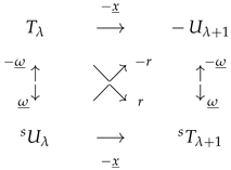
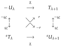
4. Signum Pairs and Cross Pairs of Operators

With each well-defined operator P acting between distributions, there corresponds an operator

$$P^{\vee }=\underline{\omega }P(-\underline{\omega })$$

acting between signumdistributions, according to the following commutative diagram defined as

in this way giving rise to a pair of operators P and $P^{\vee }$ which we call a signum pair of operators. If the operator P action result is uniquely determined, then the action result of $P^{\vee }$ is uniquely determined too, in which case we use the notation $(P,P^{\vee })$ for this signum pair of operators. If, on the contrary, the action result of P is an equivalence class of distributions, then the action result of $P^{\vee }$ will be an equivalence class of signumdistributions, in which case we use the notation $[P,P^{\vee }]$. Several signum pairs of operators are listed in

Table 1. Signum pairs of operators.

$(\underline{x},\underline{x})$
$(r^2,r^2)$
$(\mathbb{E},\mathbb{E})$
$(\mathrm{\Gamma },-{\partial }_{\underline{\omega }}\underline{\omega })$	$(-{\partial }_{\underline{\omega }}\underline{\omega },\mathrm{\Gamma })$
$({\mathrm{\Gamma }}^2,{\mathrm{\Gamma }}^2-2(m-1)\mathrm{\Gamma }+{(m-1)}^2)$	$({\mathrm{\Gamma }}^2-2(m-1)\mathrm{\Gamma }+{(m-1)}^2,{\mathrm{\Gamma }}^2)$
$(\underline{\partial },\underline{D})$	$[\underline{D},\underline{\partial }]$
$[\underline{\omega }{\partial }_r,\underline{\omega }{\partial }_r]$
$[{\displaystyle \frac{1}{r}}{\partial }_{\underline{\omega }},-{\displaystyle \frac{1}{r}}{\partial }_{\underline{\omega }}+(m-1){\displaystyle \frac{1}{r}}\underline{\omega }]$	$[-{\displaystyle \frac{1}{r}}{\partial }_{\underline{\omega }}+(m-1){\displaystyle \frac{1}{r}}\underline{\omega },{\displaystyle \frac{1}{r}}{\partial }_{\underline{\omega }}]$
$({\partial }_{\underline{\omega }}^2,{\partial }_{\underline{\omega }}^2)$
$({\Delta }^{*},{\mathbf{Z}}^{*})$	$({\mathbf{Z}}^{*},{\Delta }^{*})$
$(\Delta ,\mathbf{Z})$	$[\mathbf{Z},\Delta ]$
$[{\partial }_r^2,{\partial }_r^2]$
$[{\displaystyle \frac{1}{\underline{x}}},{\displaystyle \frac{1}{\underline{x}}}]$
$[{\displaystyle \frac{1}{r}}{\partial }_r,{\displaystyle \frac{1}{r}}{\partial }_r]$
$[{\displaystyle \frac{1}{r^2}},{\displaystyle \frac{1}{r^2}}]$
$({\partial }_{x_j},d_j)$	$[d_j,{\partial }_{x_j}]$

.

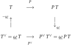
Remark 2.

When the operators P and $P^{\vee }$ form a signum pair of operators, it then follows that $P=(-\underline{\omega })P^{\vee }\underline{\omega }$, and it becomes tempting to consider the operator P as the signum partner to the operator $P^{\vee }$ and to define the action of the operator P on signumdistributions through the action of $P^{\vee }$ on distributions. However, this is justifiable only if the operator $P^{\vee }$ is a ”legal“ operator, such as a Cartesian operator, between distributions.

The above commutative diagram induces two more operators, where operator Q maps a distribution to a signumdistribution, and the corresponding operator $Q^c=(-\underline{\omega })Q(-\underline{\omega })=\underline{\omega }Q\underline{\omega }$ maps a signumdistribution to a distribution according to the following commutative diagram:

Clearly, the operators Q and $Q^c$ cannot be Cartesian, since they map distributions to signumdistributions and vice versa. We call the pair of operators Q and $Q^c$ a cross pair of operators, being denoted by either $(Q,Q^c)$ or $[Q,Q^c]$ depending on the nature of their action result, which is similar to the case of a signum pair of operators. In

Table 2. Cross pairs of operators.

$(\underline{\omega },\underline{\omega })$
$(r,-r)$	$(-r,r)$
$[{\partial }_r,-{\partial }_r]$	$[-{\partial }_r,{\partial }_r]$
$({\partial }_{\underline{\omega }},\underline{\omega }{\partial }_{\underline{\omega }}\underline{\omega })$	$(\underline{\omega }{\partial }_{\underline{\omega }}\underline{\omega },{\partial }_{\underline{\omega }})$
$[{\displaystyle \frac{1}{r}},-{\displaystyle \frac{1}{r}}]$	$[-{\displaystyle \frac{1}{r}},{\displaystyle \frac{1}{r}}]$
$[{\displaystyle \frac{1}{r}}{\partial }_{\underline{\omega }}\underline{\omega },-{\displaystyle \frac{1}{r}}\underline{\omega }{\partial }_{\underline{\omega }}]$	$[-{\displaystyle \frac{1}{r}}{\partial }_{\underline{\omega }}\underline{\omega },{\displaystyle \frac{1}{r}}\underline{\omega }{\partial }_{\underline{\omega }}]$

, several cross pairs of operators are listed.

In Section 3, we saw that the Laplace–Beltrami operator ${\Delta }^{*}$ and the square of the angular derivative ${\partial }_{\underline{\omega }}^2$ are Cartesian operators. Their signum partners are straightforwardly computed as

$$\begin{array}{c}\hfill {\left({\partial }_{\underline{\omega }}^2\right)}^{\vee }=\underline{\omega }{\partial }_{\underline{\omega }}^2(-\underline{\omega })={\partial }_{\underline{\omega }}^2\end{array}$$

and

$$\begin{array}{c}\hfill {\Delta }^{*\vee }=-{\mathrm{\Gamma }}^2+m\mathrm{\Gamma }-(m-1)\mathbf{1}.\end{array}$$

Clearly, the operator ${\Delta }^{*\vee }$ is also Cartesian. Introducing the notation ${\mathbf{Z}}^{*}={\Delta }^{*\vee }$, the signum pairs of operators $({\partial }_{\underline{\omega }}^2,{\partial }_{\underline{\omega }}^2)$, $({\Delta }^{*},{\mathbf{Z}}^{*})$, and $({\mathbf{Z}}^{*},{\Delta }^{*})$ follow, inducing the definition of the actions of the operators ${\partial }_{\underline{\omega }}^2$, ${\mathbf{Z}}^{*}$ and ${\Delta }^{*}$ on a signumdistribution.

For the signum partner $\underline{D}$ of the Dirac operator $\underline{\partial }$ we obtain the following expressions:

$$\begin{array}{ccc}\hfill \underline{D}& =& \underline{\omega }\underline{\partial }(-\underline{\omega })=\underline{\omega }(\underline{\omega }{\partial }_r+{\displaystyle \frac{1}{r}}{\partial }_{\underline{\omega }})(-\underline{\omega })\hfill \\ & =& \underline{\omega }{\partial }_r+{\displaystyle \frac{1}{r}}\underline{\omega }{\partial }_{\underline{\omega }}(-\underline{\omega })\hfill \\ & =& \underline{\omega }{\partial }_r-{\displaystyle \frac{1}{r}}{\partial }_{\underline{\omega }}+(m-1){\displaystyle \frac{1}{r}}\underline{\omega }\hfill \\ & =& \underline{\partial }-2{\displaystyle \frac{1}{r}}{\partial }_{\underline{\omega }}+(m-1){\displaystyle \frac{1}{r}}\underline{\omega }\hfill \\ & =& -\underline{\partial }+2\underline{\omega }{\partial }_r+(m-1){\displaystyle \frac{1}{r}}\underline{\omega },\hfill \end{array}$$

giving rise to the signum pairs of operators $(\underline{\partial },\underline{D})$ and $[{\displaystyle \frac{1}{r}}{\partial }_{\underline{\omega }},-{\displaystyle \frac{1}{r}}{\partial }_{\underline{\omega }}+(m-1){\displaystyle \frac{1}{r}}\underline{\omega }]$, which induce the actions of operators $\underline{D}$ and $-{\displaystyle \frac{1}{r}}{\partial }_{\underline{\omega }}+(m-1){\displaystyle \frac{1}{r}}\underline{\omega }$ on a signumdistribution.

Note that while the actions of the operator $\underline{\partial }$ on distributions and of its signum partner $\underline{D}$ on signumdistributions are uniquely determined, the action results of operator ${\displaystyle \frac{1}{r}}{\partial }_{\underline{\omega }}$ on distributions and of its signum partner $-{\displaystyle \frac{1}{r}}{\partial }_{\underline{\omega }}+(m-1){\displaystyle \frac{1}{r}}\underline{\omega }$ on signumdistributions are equivalent classes.

We call operator $\underline{D}$ the signum-Dirac operator. At first sight, it is not clear if $\underline{D}$ is Cartesian. However, this is indeed true, and we have the following result:

Proposition 3.

The operators $\underline{D}$ and $-{\displaystyle \frac{1}{r}}{\partial }_{\underline{\omega }}+(m-1){\displaystyle \frac{1}{r}}\underline{\omega }$ are Cartesian operators.

Proof. 

In view of Definition 2 it holds that

$$-{\displaystyle \frac{1}{r}}{\partial }_{\underline{\omega }}+(m-1){\displaystyle \frac{1}{r}}\underline{\omega }={\displaystyle \frac{1}{\underline{x}}}(\mathrm{\Gamma }-(m-1)\mathbf{1})$$

and also

$$\begin{array}{ccc}\hfill \underline{D}& =& {\displaystyle \frac{1}{\underline{x}}}(-\mathbb{E}+\mathrm{\Gamma }-(m-1)\mathbf{1})\hfill \\ & =& \underline{\partial }+{\displaystyle \frac{1}{\underline{x}}}(2\mathrm{\Gamma }-(m-1)\mathbf{1})\hfill \\ & =& -\underline{\partial }+{\displaystyle \frac{1}{\underline{x}}}(-2\mathbb{E}-(m-1)\mathbf{1}).\hfill \end{array}$$

□

This leads to a signum pair of operators $[\underline{D},\underline{\partial }]$, which induces the action of the Dirac operator $\underline{\partial }$ on a signumdistribution. However, owing to division by $\underline{x}$, the latter action results into an equivalence class of signumdistributions.

It is interesting to note that, in the same way as the Dirac operator factorizes the Laplace operator, ${\underline{\partial }}^2=-\Delta$, the signum-Dirac operator $\underline{D}$ factorizes the signum-Laplace operator, i.e., the signum partner of the Laplace operator:

$${\underline{D}}^2={\left(\underline{\omega }\underline{\partial }(-\underline{\omega })\right)}^2=\underline{\omega }{\underline{\partial }}^2(-\underline{\omega })=-\underline{\omega }\Delta (-\underline{\omega })=-{\Delta }^{\vee }.$$

Introducing the notation $\mathbf{Z}={\Delta }^{\vee }$, it follows that $(\Delta ,\mathbf{Z})$ is a signum pair of operators, with

$$\begin{array}{ccc}\hfill \mathbf{Z}& =& -{\underline{D}}^2\hfill \\ & =& {\partial }_r^2+(m-1){\displaystyle \frac{1}{r}}{\partial }_r+{\displaystyle \frac{1}{r^2}}{\mathbf{Z}}^{*}.\hfill \end{array}$$

Clearly, operator $\mathbf{Z}$ is Cartesian. The signum pair of operators $[\mathbf{Z},\Delta ]$ follows, inducing the action of Laplace operator $\Delta$ on a signumdistribution.

From Section 3, we know that the operators ${\partial }_r^2$, ${\displaystyle \frac{1}{r}}{\partial }_r$, and ${\displaystyle \frac{1}{r^2}}{\Delta }^{*}$, which are constituents of the Laplace operator $\Delta$, are Cartesian operators. Their signum partners are easily seen as

$$\begin{array}{ccc}\hfill {\left({\partial }_r^2\right)}^{\vee }& =& {\partial }_r^2\hfill \\ \hfill {\left({\displaystyle \frac{1}{r}}{\partial }_r\right)}^{\vee }& =& {\displaystyle \frac{1}{r}}{\partial }_r\hfill \\ \hfill {\left({\displaystyle \frac{1}{r^2}}{\Delta }^{*}\right)}^{\vee }& =& {\displaystyle \frac{1}{r^2}}{\mathbf{Z}}^{*},\hfill \end{array}$$

and the signum pairs of operators $[{\partial }_r^2,{\partial }_r^2]$, $[{\displaystyle \frac{1}{r}}{\partial }_r,{\displaystyle \frac{1}{r}}{\partial }_r]$, $[{\displaystyle \frac{1}{r^2}}{\Delta }^{*},{\displaystyle \frac{1}{r^2}}{\mathbf{Z}}^{*}]$, and $[{\displaystyle \frac{1}{r^2}}{\mathbf{Z}}^{*},{\displaystyle \frac{1}{r^2}}{\Delta }^{*}]$ follow, inducing the actions of the operators ${\partial }_r^2$, ${\displaystyle \frac{1}{r}}{\partial }_r$, ${\displaystyle \frac{1}{r^2}}{\mathbf{Z}}^{*}$, and ${\displaystyle \frac{1}{r^2}}{\Delta }^{*}$ on a signumdistribution.

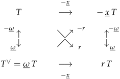
5. Spherical Operators

We say that an operator involving the spherical coordinates is spherical when it is not Cartesian. Clearly, the multiplication operators r and $\underline{\omega }$ are spherical operators, as are the differential operators ${\partial }_r$ and ${\partial }_{\underline{\omega }}$. The concepts of signumdistribution, signum pair of operators, and cross pair of operators allow for the definition of the action of spherical operators on both distributions and signumdistributions.

Definition 3.

The product of a distribution T by the function $\underline{\omega }$ is the signumdistribution $T^{\vee }$ associated with T, and, for all test functions $\underline{\omega }\phi \in \mathrm{\Omega }({\mathbb{R}}^m;{\mathbb{R}}^m)$, it holds that

$$\langle \underline{\omega }T,\underline{\omega }\phi \rangle =\langle T^{\vee },\underline{\omega }\phi \rangle =-\langle T,\phi \rangle .$$

Similarly, the product of the signumdistribution ${}^{s}U$ by the function $(-\underline{\omega })$ is its associated distribution ${}^{s}U^{\wedge }$, and it holds that

$$\langle (-\underline{\omega }){}^{s}U,\phi \rangle =\langle {}^{s}U^{\wedge },\phi \rangle =-\langle {}^{s}U,\underline{\omega }\phi \rangle .$$

Definition 4.

The product of a scalar distribution $T^{scal}$ by the function ${\omega }_j,j=1,\dots ,m$ is the signumdistribution ${\omega }_j{T}^{scal}$ given by the uniquely determined expression

$${\omega }_j{T}^{scal}={}_j{}^{\left\{\underline{\omega }{T}^{scal}\right\}}.$$

Similarly, the product of the scalar signumdistribution ${}^{s}U^{scal}$ by the function ${\omega }_j$ is the distribution ${\omega }_j{}^{s}U^{scal}$ given by

$${\omega }_j{}^{s}U^{scal}={\left\{\underline{\omega }{}^{s}U^{scal}\right\}}_j.$$

Remark 3.

For a general Clifford algebra-valued distribution or signumdistribution, the action of the multiplicative operator ${\omega }_j$ is defined through linearity with respect to the scalar components.

Definition 5.

The product of a scalar distribution T by the function r is the signumdistribution $rT={(-\underline{x}T)}^{\vee }$ given for all test functions $\underline{\omega }\phi \in \mathrm{\Omega }({\mathbb{R}}^m;{\mathbb{R}}^m)$ by

$$\langle rT,\underline{\omega }\phi \rangle =\langle \underline{x}T,\phi \rangle =\langle T,\underline{x}\phi \rangle ,$$

according to the upper triangular part of the commutative diagram

involving the signum pair of operators $(\underline{x},\underline{x})$, which induces the product of the signumdistribution $\underline{\omega }T$ by $\underline{x}$ to be $\underline{x}\left(\underline{\omega }T\right)=-rT$.

Definition 6.

The derivative with respect to the radial distance r of a scalar distribution T is the equivalent class of signumdistributions

$$\left[{\partial }_{r}T\right]={\left[-\underline{\omega }{\partial }_{r}T\right]}^{\vee }={\left[{\displaystyle \frac{1}{\underline{x}}}\mathbb{E}T\right]}^{\vee }={\left(\underline{S}+\underline{c}\delta \left(\underline{x}\right)\right)}^{\vee }=\underline{\omega }\underline{S}+\underline{\omega }\delta \left(\underline{x}\right)\underline{c},$$

for any vector distribution $\underline{S}$ satisfying $\underline{x}\underline{S}=\mathbb{E}T$, according to the upper triangular part of the commutative diagram

involving the signum pair of operators $[\underline{\omega }{\partial }_r,\underline{\omega }{\partial }_r]$, which induces the action of $\left(\underline{\omega }{\partial }_r\right)$ on the signumdistribution $\underline{\omega }T$ to be $\left(\underline{\omega }{\partial }_r\right)\left(\underline{\omega }T\right)=[-{\partial }_{r}T]$.

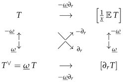
Definition 7.

The angular ${\partial }_{\underline{\omega }}$-derivative of a distribution T is the unique signumdistribution ${\partial }_{\underline{\omega }}T={\left(\mathrm{\Gamma }T\right)}^{\vee }$ given for all test functions $\underline{\omega }\phi \in \mathrm{\Omega }({\mathbb{R}}^m;{\mathbb{R}}^m)$ by

$$\langle \underline{\omega }\phi ,{\partial }_{\underline{\omega }}T\rangle =\langle \phi ,\underline{\omega }{\partial }_{\underline{\omega }}T\rangle =\langle \phi ,-\mathrm{\Gamma }T\rangle ,$$

according to the upper triangular part of the commutative diagram

involving the signumpair of operators $(\underline{\omega }{\partial }_{\underline{\omega }},{\partial }_{\underline{\omega }}\underline{\omega })$ or $(\mathrm{\Gamma },-{\partial }_{\underline{\omega }}\underline{\omega })=(\mathrm{\Gamma },(m-1)\mathbf{1}-\mathrm{\Gamma })$, which induces the action of the operator ${\partial }_{\underline{\omega }}\underline{\omega }$ on the signumdistribution $\underline{\omega }T$ to be ${\partial }_{\underline{\omega }}\underline{\omega }\left(\underline{\omega }T\right)=-{\partial }_{\underline{\omega }}T$.

Definition 8.

The angular ${\partial }_{{\omega }_j}$-derivative of a scalar distribution $T^{scal}$ is the unique signumdistribution given by

$${\partial }_{{\omega }_j}{T}^{scal}={\left\{{\partial }_{\underline{\omega }}{T}^{scal}\right\}}_j,j=1,\dots ,m.$$

Remark 4.

(i) 

An alternative expression for ${\partial }_{{\omega }_j}{T}^{scal}$ is

$${\partial }_{{\omega }_j}{T}^{scal}=r{\partial }_{x_j}{T}^{scal}-{\omega }_j\mathbb{E}{T}^{scal}.$$

Indeed, it follows from

$$-\mathrm{\Gamma }{T}^{scal}=\underline{x}\underline{\partial }{T}^{scal}+\mathbb{E}{T}^{scal}$$

that

$$-{\partial }_{\underline{\omega }}{T}^{scal}=-\underline{\omega }\underline{x}\underline{\partial }{T}^{scal}+\underline{\omega }\mathbb{E}{T}^{scal}=-r\underline{\partial }{T}^{scal}+\underline{\omega }\mathbb{E}{T}^{scal}$$

whence we have the desired formula states for each of the components.

(ii) 

For a general Clifford algebra-valued distribution, the action of the spherical derivative operator ${\partial }_{{\omega }_j}$ is defined through linearity with respect to the scalar components.

Definition 9.

The quotient of a scalar distribution T by the radial distance r is the equivalence class of the signumdistributions

$$\left[{\displaystyle \frac{1}{r}}T\right]=\underline{\omega }\left[{\displaystyle \frac{1}{\underline{x}}}T\right]=\underline{\omega }(\underline{S}+\delta \left(\underline{x}\right)\underline{c})=\underline{\omega }\underline{S}+\underline{\omega }\delta \left(\underline{x}\right)\underline{c}={\underline{S}}^{\vee }+\delta {\left(\underline{x}\right)}^{\vee }\underline{c},$$

for any vector-valued distribution $\underline{S}$ for which $\underline{x}\underline{S}=T$, according to the upper triangular part of the commutative diagram

involving the signum pair of operators $[{\displaystyle \frac{1}{\underline{x}}},{\displaystyle \frac{1}{\underline{x}}}]$, which induces the quotient of the signumdistribution $\underline{\omega }T$ by $\underline{x}$ to be ${\displaystyle \frac{1}{\underline{x}}}\left(\underline{\omega }T\right)=\left[{\displaystyle \frac{1}{r}}T\right]$.

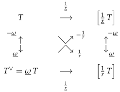
Remark 5.

Once the action of the spherical derivative operators ${\partial }_{{\omega }_j},j=1,\dots ,m$ is defined in Definition 8, we are able to define the action of the corresponding Cartesian operators $-\underline{\omega }{\partial }_{{\omega }_j},j=1,\dots ,m$ through the commutative diagram

In particular, for a scalar distribution $T^{scal}$, it holds that

$$-\underline{\omega }{\partial }_{{\omega }_j}{T}^{scal}=-\underline{x}{\partial }_{x_j}{T}^{scal}+{\omega }_j\underline{\omega }\mathbb{E}{T}^{scal},j=1,\dots ,m.$$

Example 1.

Because $\delta \left(\underline{x}\right)$ is a radial distribution, we expect ${\partial }_{{\omega }_j}\delta \left(\underline{x}\right)$, and thus also $-\underline{\omega }{\partial }_{{\omega }_j}\delta \left(\underline{x}\right)$, to be zero. And indeed it holds that

$$\begin{array}{cc}\hfill {\partial }_{{\omega }_j}\delta \left(\underline{x}\right)& =r{\partial }_{x_j}\delta \left(\underline{x}\right)-{\omega }_j\mathbb{E}\delta \left(\underline{x}\right)\hfill \\ \hfill & =r{\partial }_{x_j}\delta \left(\underline{x}\right)+m{\omega }_j\delta \left(\underline{x}\right)\hfill \\ \hfill & ={\{r\underline{\partial }\delta \left(\underline{x}\right)+m\underline{\omega }\delta \left(\underline{x}\right)\}}_j\hfill \\ \hfill & ={\{\underline{\omega }\mathbb{E}\delta \left(\underline{x}\right)+m\underline{\omega }\delta \left(\underline{x}\right)\}}_j\hfill \\ \hfill & =0.\hfill \end{array}$$

6. Action Uniqueness of Some Operators

In the preceding sections, we encountered operators acting on distributions and on signumdistributions with a uniquely determined result and those whose actions were not uniquely determined but instead lead to equivalence classes of distributions and signumdistributions, respectively. Nevertheless, in [6], sufficient conditions were found to guarantee the uniqueness of the latter operators’ actions involving homogeneous, radial, and signum-radial distributions and signumdistributions.

Definition 10.

(i) A distribution T or a signumdistribution ${}^{s}U$ is said to be radial if it is SO$\left(m\right)$-invariant and depends only on $r=|\underline{x}|$: $T\left(\underline{x}\right)=T\left(r\right)$ or ${}^{s}U\left(\underline{x}\right)={}^{s}U\left(r\right)$, respectively. (ii) A distribution and signumdistribution are said to be signum-radial if their associated signumdistribution and distribution, respectively, are radial.

For the sake of completeness, we recall these sufficient conditions.

(i)

If the distribution $T^{rad}$ is radial, then the following actions are uniquely determined as

$$\left(\underline{\omega }{\partial }_r\right)T^{rad},\left(-{\displaystyle \frac{1}{r}}{\partial }_{\underline{\omega }}+(m-1){\displaystyle \frac{1}{r}}\underline{\omega }\right)T^{rad},{\displaystyle \frac{1}{\underline{x}}}{T}^{rad},\underline{D}{T}^{rad},{\partial }_r{T}^{rad},{\displaystyle \frac{1}{r}}{T}^{rad}$$

and the actions of the corresponding signum partner operators on the signum-radial signumdistribution ${}^{s}U^{srad}$

$$\left(\underline{\omega }{\partial }_r\right){}^{s}U^{srad},\left({\displaystyle \frac{1}{r}}{\partial }_{\underline{\omega }}\right){}^{s}U^{srad},{\displaystyle \frac{1}{\underline{x}}}{}^{s}U^{srad},\underline{\partial }{}^{s}U^{srad},{\partial }_r{}^{s}U^{srad},{\displaystyle \frac{1}{r}}{}^{s}U^{srad}$$

are also uniquely determined.

(ii)

If the distribution $T^{\left(k\right)}$ is homogeneous with homogeneity degree $k\ne -m+1$, then the following actions are uniquely determined:

$$\left(\underline{\omega }{\partial }_r\right)T^{\left(k\right)},\left({\displaystyle \frac{1}{r}}{\partial }_{\underline{\omega }}\right)T^{\left(k\right)},\left(-{\displaystyle \frac{1}{r}}{\partial }_{\underline{\omega }}+(m-1){\displaystyle \frac{1}{r}}\underline{\omega }\right)T^{\left(k\right)},{\displaystyle \frac{1}{\underline{x}}}{T}^{\left(k\right)},$$

and

$$\underline{D}{T}^{\left(k\right)},{\partial }_r{T}^{\left(k\right)},{\displaystyle \frac{1}{r}}{T}^{\left(k\right)}$$

Additionally, the actions of the corresponding signum partner operators on the homogeneous signumdistribution ${}^{s}U^{\left(k\right)}$, viz.,

$$\left(\underline{\omega }{\partial }_r\right){}^{s}U^{\left(k\right)},\left(-{\displaystyle \frac{1}{r}}{\partial }_{\underline{\omega }}+(m-1){\displaystyle \frac{1}{r}}\underline{\omega }\right){}^{s}U^{\left(k\right)},\left({\displaystyle \frac{1}{r}}{\partial }_{\underline{\omega }}\right){}^{s}U^{\left(k\right)},{\displaystyle \frac{1}{\underline{x}}}{}^{s}U^{\left(k\right)},\underline{\partial }{}^{s}U^{\left(k\right)},$$

and

$${\partial }_r{}^{s}U^{\left(k\right)},{\displaystyle \frac{1}{r}}{}^{s}U^{\left(k\right)},$$

are also uniquely determined.

(iii)

If the distribution $T^{\left(k\right)}$ is homogeneous with homogeneity degree $k\ne -m+1,-m+2$, then the following actions are uniquely determined:

$${\partial }_r^2{T}^{\left(k\right)},{\displaystyle \frac{1}{r}}{\partial }_r{T}^{\left(k\right)},{\displaystyle \frac{1}{r^2}}{\Delta }^{*}{T}^{\left(k\right)},{\displaystyle \frac{1}{r^2}}{\mathbf{Z}}^{*}{T}^{\left(k\right)},\mathbf{Z}{T}^{\left(k\right)},{\displaystyle \frac{1}{r^2}}{T}^{\left(k\right)}$$

and the actions of the corresponding signum partner operators on the homogeneous signumdistribution ${}^{s}U^{\left(k\right)}$

$${\partial }_r^2{}^{s}U^{\left(k\right)},{\displaystyle \frac{1}{r}}{\partial }_r{}^{s}U^{\left(k\right)},{\displaystyle \frac{1}{r^2}}{\mathbf{Z}}^{*}{}^{s}U^{\left(k\right)},{\displaystyle \frac{1}{r^2}}{\Delta }^{*}{}^{s}U^{\left(k\right)},\Delta {}^{s}U^{\left(k\right)},{\displaystyle \frac{1}{r^2}}{}^{s}U^{\left(k\right)}$$

are uniquely determined as well.

(iv)

The conclusions contained in (iii) remain valid if the distribution and signumdistribution under consideration are both radial and signum-radial, respectively, and homogeneous with homogeneity degree $k\ne -m+2$.

(v)

The conclusions contained in (iii) remain valid if the distribution and signumdistribution under consideration are both signum-radial and radial, respectively, and homogeneous with homogeneity degree $k\ne -m+1$.

7. Cartesian Derivatives of Signumdistributions

Recalling the signum pairs of operators $(\underline{\partial },\underline{D})$ and $[\underline{D},\underline{\partial }]$, we expect the Cartesian derivatives of distributions and of signumdistributions to appear in the signum pairs of operators of the form $({\partial }_{x_j},d_j)$ and $[d_j,{\partial }_{x_j}]$, $j=1,\dots ,m$. Operators $d_j,j=1,\dots ,m$ are important in the following sense: When defining a derivative of a distribution, which is merely a sophisticated integration by parts, the differential operator, say ${\partial }_{x_j}$, shifts to the test function. It was shown in [6] that when computing the derivative ${\partial }_{x_j}$ of a signumdistribution, the derivative shifts to the test function, but in the form of the operator $d_j$.

Definition 11.

For $j=1,\dots ,m$, we define operator $d_j$ as the signum partner of the Cartesian derivative ${\partial }_{x_j}$, and it holds that

$$\begin{array}{ccc}\hfill d_j& =& \underline{\omega }{\partial }_{x_j}(-\underline{\omega })\hfill \\ & =& -{\displaystyle \frac{1}{r}}\underline{\omega }{e}_j-{\displaystyle \frac{1}{r}}{\omega }_j+{\partial }_{x_j}={\displaystyle \frac{1}{r}}{e}_j\underline{\omega }+{\displaystyle \frac{1}{r}}{\omega }_j+{\partial }_{x_j}\hfill \\ & =& -{\displaystyle \frac{1}{r^2}}\underline{x}{e}_j-{\displaystyle \frac{1}{r^2}}{x}_j+{\partial }_{x_j}={\displaystyle \frac{1}{r^2}}{e}_j\underline{x}+{\displaystyle \frac{1}{r^2}}{x}_j+{\partial }_{x_j}\hfill \\ & =& {\displaystyle \frac{1}{\underline{x}}}{e}_j+(-{\displaystyle \frac{x_j}{r^2}})+{\partial }_{x_j}=-e_j{\displaystyle \frac{1}{\underline{x}}}-(-{\displaystyle \frac{x_j}{r^2}})+{\partial }_{x_j}.\hfill \end{array}$$

Clearly, each of the operators $d_j(j=1,\dots ,m)$ is Cartesian. It is the sum of the scalar part ${\partial }_{x_j}$ and bivector part ${\displaystyle \frac{1}{r^2}}{e}_j\underline{x}+{\displaystyle \frac{1}{r^2}}{x}_j={\displaystyle \frac{1}{r^2}}(e_j{e}_1{x}_1+\dots +e_j{e}_{j-1}{x}_{j-1}+e_j{e}_{j+1}{x}_{j+1}+\dots +e_j{e}_m{x}_m)$. This bivector part is a combination of the operator ${\displaystyle \frac{1}{\underline{x}}}$ and its components $(-{\displaystyle \frac{j}{r^2}},j=1,\dots ,m)$.

As the operator $d_j$ is a well-defined, but not uniquely defined, operator acting on distributions, the signum pairs of operators $[d_j,{\partial }_{x_j}]$, $j=1,\dots ,m$ hold, enabling the definition of the Cartesian derivative ${\partial }_{x_j}$ of a signumdistribution as an equivalence class of signumdistributions, as shown in the following commutative diagram:

Remark 6.

A relationship exists between operators $d_j,j=1,\dots ,m$, Dirac operator $\underline{\partial }$, and operator $\underline{D}$. A straightforward calculation is as follows:

$$\begin{array}{ccc}\hfill \underline{\partial }& =& \phantom{-}\sum _{j=1}^m{e}_j{d}_j+(m-1){\displaystyle \frac{1}{r^2}}\underline{x}=\phantom{-}\sum _{j=1}^m{e}_j{d}_j-(m-1){\displaystyle \frac{1}{\underline{x}}},\hfill \\ \hfill \underline{D}& =& -\sum _{j=1}^m{e}_j{d}_j+2{\displaystyle \frac{1}{r^2}}\underline{x}\mathbb{E}=-\sum _{j=1}^m{e}_j{d}_j-2{\displaystyle \frac{1}{\underline{x}}}\mathbb{E}.\hfill \end{array}$$

8. Actions on ${\mathit{T}}_{\mathit{\lambda }}$ and ${\mathit{U}}_{\mathit{\lambda }}$

The results of the preceding sections now will be applied to the distributions $T_{\lambda }$ and $U_{\lambda }$. Recalling Definition 1, for $\lambda \in \mathbb{C}$, it holds that

$$\langle T_{\lambda },\phi \left(\underline{x}\right)\rangle :=a_m\langle \mathrm{Fp}{r}_{+}^{\lambda +m-1},{\Sigma }^{\left(0\right)}\left[\phi \right]\left(r\right)\rangle$$

and

$$\langle U_{\lambda },\phi \left(\underline{x}\right)\rangle :=a_m\langle \mathrm{Fp}{r}_{+}^{\lambda +m-1},{\Sigma }^{\left(1\right)}\left[\phi \right]\left(r\right)\rangle .$$

An alternative, and handy, notation could be $T_{\lambda }=\mathrm{Fp}{r}^{\lambda }$ and $U_{\lambda }=\underline{\omega }\mathrm{Fp}{r}^{\lambda }$.

For more details, we refer to the series of papers cited at the beginning of Section 1 and also to Appendix B. Now, we briefly comment on Definition 1.

A priori, the distributions $T_{\lambda }$ and $U_{\lambda }$ are not defined at the simple poles $\lambda =-m-n+1$, $n\in \mathbb{N}$, on the r-axis, of the one-dimensional distribution Fp$r_{+}^{\lambda +m-1}$. To cope with these singularities, the distributions Fp$r_{+}^{-n}$, $n\in \mathbb{N}$ are interpreted as monomial pseudofunctions (see Appendix A).

The distributions $T_{\lambda }$ are standard scalar distributions that are well known in harmonic analysis. They are radial and homogeneous of degree $\lambda$. As meromorphic functions of $\lambda \in \mathbb{C}$, they exhibit genuine simple poles at $\lambda =-m,-m-2,-m-4,\dots$. This is due to the fact that the singular points $\lambda =-m-2\ell -1$, $\ell =0,1,2,\dots$ are removable, since the spherical mean ${\Sigma }^{\left(0\right)}\left[\varphi \right]$ has its odd-order derivatives vanishing at $r=0$. So, we can define

$$\langle T_{-m-2\ell -1},\varphi \rangle =\underset{\mu \to -2\ell -2}{lim}{a}_m\langle \mathrm{Fp}{r}_{+}^{\mu },{\Sigma }^{\left(0\right)}\left[\varphi \right]\left(r\right)\rangle$$

but, remarkably, this limit is precisely $a_m\langle \mathrm{Fp}{r}_{+}^{-2\ell -2},{\Sigma }^{\left(0\right)}\left[\varphi \right]\left(r\right)\rangle$, with Fp$r_{+}^{-2\ell -2}$ being the monomial pseudofunction. The most important distribution in this family is $T_{-m+2}={\displaystyle \frac{1}{r^{m-2}}}$, which is, up to a constant, the fundamental solution of the Laplace operator $\Delta$. Also, note the special cases $T_0=1$, $T_{2\ell }=r^{2\ell }={(-1)}^{\ell }{\underline{x}}^{2\ell }$ and $T_{2\ell +1}=r^{2\ell +1},\ell =0,1,2,\dots$.

The distributions $U_{\lambda }$ are homogeneous of degree $\lambda$. As vector-valued meromorphic functions of $\lambda \in \mathbb{C}$, they exhibit genuine simple poles at $\lambda =-m-1,-m-3,-m-5,\dots$. This is due to the fact that the singular points $\lambda =-m-2\ell$, $\ell =0,1,2,\dots$ are removable, since the spherical mean ${\Sigma }^{\left(1\right)}\left[\varphi \right]$ has its even-order derivatives vanishing at $r=0$. So, we can define

$$\langle U_{-m-2\ell },\varphi \rangle =\underset{\mu \to -2\ell -1}{lim}{a}_m\langle \mathrm{Fp}{r}_{+}^{\mu },{\Sigma }^{\left(1\right)}\left[\varphi \right]\rangle ,$$

but this limit is precisely $a_m\langle \mathrm{Fp}{r}_{+}^{-2\ell -1},{\Sigma }^{\left(1\right)}\left[\varphi \right]\rangle$, with Fp$r_{+}^{-2\ell -1}$ being the monomial pseudofunction. The most important distribution in this family is $U_{-m+1}={\displaystyle \frac{\underline{\omega }}{r^{m-1}}}={\displaystyle \frac{\underline{x}}{r^m}}$, which is, up to a constant, the fundamental solution of the Dirac operator $\underline{\partial }$. Also, note the special cases $U_0=\underline{\omega }$, $U_{2\ell }=\underline{\omega }{r}^{2\ell }$ and $U_{2\ell +1}=\underline{\omega }{r}^{2\ell +1}={(-1)}^{\ell }{\underline{x}}^{2\ell +1},\ell =0,1,2,\dots$.

It is important to note that, although the distributions $T_{\lambda }$ and $U_{\lambda }$ are also defined in their respective singularities, these exceptional values do not turn these distributions into entire functions of parameter $\lambda \in \mathbb{C}$.

When restricted to the half-plane $\mathbb{R}e\lambda >-m$, the distributions $T_{\lambda }$ and $U_{\lambda }$ are regular, that is, they are locally integrable functions. From [3,5,6], we know that a locally integrable function can also be seen as a signumdistribution. This inspires the definition of the following two families of the following signumdistributions:

$$\langle {}^{s}T_{\lambda },\underline{\omega }\phi \left(\underline{x}\right)\rangle :=\phantom{-}{a}_m\langle \mathrm{Fp}{r}_{+}^{\lambda +m-1},{\Sigma }^{\left(1\right)}\left[\phi \right]\left(r\right)\rangle$$

and

$$\langle {}^{s}U_{\lambda },\underline{\omega }\phi \left(\underline{x}\right)\rangle :=-a_m\langle \mathrm{Fp}{r}_{+}^{\lambda +m-1},{\Sigma }^{\left(0\right)}\left[\phi \right]\left(r\right)\rangle .$$

It is clear that

$$T_{\lambda }^{\vee }=\phantom{-}{}^{s}U_{\lambda },{}^{s}U_{\lambda }^{\wedge }=\phantom{-}{T}_{\lambda },$$

and

$$U_{\lambda }^{\vee }=-{}^{s}T_{\lambda },{}^{s}T_{\lambda }^{\wedge }=-U_{\lambda }.$$

Thus, ${}^{s}T_{\lambda }$ inherits the simple poles of $U_{\lambda }$, that is, $\lambda =-m-1,-m-3,-m-5,\dots$, whereas ${}^{s}U_{\lambda }$ inherits the simple poles of $T_{\lambda }$, that is, $\lambda =-m,-m-2,-m-4,\dots$.

Because the distributions $T_{\lambda }$ are radial, according to Definition 10, the signumdistributions ${}^{s}U_{\lambda }$ are signum-radial. Because the signumdistributions ${}^{s}T_{\lambda }$ are radial, and by the same definition, the distributions $U_{\lambda }$ are signum-radial.

In the following subsections, we systematically compute the actions on $T_{\lambda }$, $U_{\lambda }$, ${}^{s}T_{\lambda }$, and ${}^{s}U_{\lambda }$ of all operators introduced in the preceding sections, paying attention to the uniqueness of the expressions obtained.

8.1. The Operators $\underline{x}$, r, and $r^2$

The multiplication operator $\underline{x}$ is a Cartesian operator whose actions are, naturally, uniquely determined. For all $\lambda \in \mathbb{C}$, it holds that

$$\begin{array}{|c|}\hline \underline{x}{T}_{\lambda }=U_{\lambda +1}\\ \hline\end{array},\begin{array}{|c|}\hline \underline{x}{U}_{\lambda }=-T_{\lambda +1}\\ \hline\end{array}.$$

(6)

Based on the commutative diagram

we find the additional formulæ

$$\begin{array}{|c|}\hline r{T}_{\lambda }={}^{s}T_{\lambda +1}\\ \hline\end{array}\mathrm{and}\begin{array}{|c|}\hline r{}^{s}U_{\lambda }=U_{\lambda +1}\\ \hline\end{array},\lambda \in \mathbb{C},$$

and

$$\begin{array}{|c|}\hline \underline{x}{}^{s}U_{\lambda }=-{}^{s}T_{\lambda +1}\\ \hline\end{array},\lambda \in \mathbb{C}.$$

Similarly, based on the commutative diagram

we obtain the additional formulæ

$$\begin{array}{|c|}\hline r{}^{s}T_{\lambda }=T_{\lambda +1}\\ \hline\end{array}\mathrm{and}\begin{array}{|c|}\hline r{U}_{\lambda }={}^{s}U_{\lambda +1}\\ \hline\end{array},\lambda \in \mathbb{C},$$

and also

$$\begin{array}{|c|}\hline \underline{x}{}^{s}T_{\lambda }={}^{s}U_{\lambda +1}\\ \hline\end{array},\lambda \in \mathbb{C}.$$

Iteration of the multiplication operator $\underline{x}$ results in

$$\begin{array}{|c|}\hline r^2{T}_{\lambda }=T_{\lambda +2}\\ \hline\end{array},\begin{array}{|c|}\hline r^2{U}_{\lambda }=U_{\lambda +2}\\ \hline\end{array},\lambda \in \mathbb{C},$$

and

$$\begin{array}{|c|}\hline r^2{}^{s}T_{\lambda }={}^{s}T_{\lambda +2}\\ \hline\end{array},\begin{array}{|c|}\hline r^2{}^{s}U_{\lambda }={}^{s}U_{\lambda +2}\\ \hline\end{array},\lambda \in \mathbb{C}.$$

The natural powers of $\underline{x}$ are Cartesian operators too. We find that, for all $\lambda \in \mathbb{C}$,

$$\begin{array}{cc}\hfill {(-1)}^{\ell }{\underline{x}}^{2\ell }{T}_{\lambda }& =r^{2\ell }{T}_{\lambda }=T_{\lambda +2\ell }\hfill \\ \hfill {(-1)}^{\ell }{\underline{x}}^{2\ell +1}{T}_{\lambda }& =\left(\underline{\omega }{r}^{2\ell +1}\right)T_{\lambda }=U_{\lambda +2\ell +1}\hfill \end{array}$$

and

$$\begin{array}{cc}\hfill {(-1)}^{\ell }{\underline{x}}^{2\ell }{U}_{\lambda }& =r^{2\ell }{U}_{\lambda }=U_{\lambda +2\ell }\hfill \\ \hfill {(-1)}^{\ell +1}{\underline{x}}^{2\ell +1}{U}_{\lambda }& =-\left(\underline{\omega }{r}^{2\ell +1}\right)U_{\lambda }=T_{\lambda +2\ell +1}.\hfill \end{array}$$

Through the appropriate commutative diagrams we find, for all $\lambda \in \mathbb{C}$,

$$\begin{array}{cc}\hfill r^{2\ell }{}^{s}T_{\lambda }& ={}^{s}T_{\lambda +2\ell }\hfill \\ \hfill r^{2\ell }{}^{s}U_{\lambda }& ={}^{s}U_{\lambda +2\ell }\hfill \end{array}$$

and

$$\begin{array}{cc}\hfill r^{2\ell +1}{T}_{\lambda }& ={}^{s}T_{\lambda +2\ell +1}\hfill \\ \hfill r^{2\ell +1}{U}_{\lambda }& ={}^{s}U_{\lambda +2\ell +1}.\hfill \end{array}$$

8.2. The Operators $\underline{\partial }$ and $\Delta$

Similar to the multiplication operator $\underline{x}$, the Dirac operator $\underline{\partial }$ intertwines the $T_{\lambda }$ and $U_{\lambda }$ distribution families. It is clearly a Cartesian operator whose action is uniquely determined. It holds that

$$\begin{array}{|c|}\hline \underline{\partial }{T}_{\lambda }=\lambda U_{\lambda -1}\\ \hline\end{array},\lambda \ne -m,-m-2,-m-4,\dots$$

(7)

and

$$\begin{array}{|c|}\hline \underline{\partial }{U}_{\lambda }=-(\lambda +m-1)T_{\lambda -1}\\ \hline\end{array},\lambda \ne -m+1,-m-1,-m-3,\dots ,$$

(8)

while for $\ell =0,1,2,\dots$,

$$\begin{array}{|c|}\hline \underline{\partial }{T}_{-m-2\ell }=-(m+2\ell )U_{-m-2\ell -1}+{(-1)}^{\ell +1}{\displaystyle \frac{1}{C(m,\ell )}}{a}_m{\underline{\partial }}^{2\ell +1}\delta \left(\underline{x}\right)\\ \hline\end{array}$$

(9)

and

$$\begin{array}{|c|}\hline \underline{\partial }{U}_{-m-2\ell +1}=(2\ell )T_{-m-2\ell }+{(-1)}^{\ell -1}{\displaystyle \frac{m+2\ell }{C(m,\ell )}}{a}_m{\underline{\partial }}^{2\ell }\delta \left(\underline{x}\right)\\ \hline\end{array},$$

(10)

with

$$C(m,\ell )=2^{2\ell +1}\ell !{\displaystyle \frac{\mathrm{\Gamma }(\frac{m}{2}+\ell +1)}{\mathrm{\Gamma }\left(\frac{m}{2}\right)}}=2^{\ell }\ell !m(m+2)(m+4)\dots (m+2\ell ).$$

In particular, for $\ell =0$, it holds that

$$\begin{array}{|c|}\hline \underline{\partial }{T}_{-m}=(-m)U_{-m-1}-{\displaystyle \frac{1}{m}}{a}_m\underline{\partial }\delta \left(\underline{x}\right)\\ \hline\end{array}$$

(11)

and

$$\begin{array}{|c|}\hline \underline{\partial }{U}_{-m+1}=-a_m\delta \left(\underline{x}\right)\\ \hline\end{array}.$$

(12)

Equation (12) expresses the well-known fact that $-{\displaystyle \frac{1}{m}}{U}_{-m+1}$ is indeed the fundamental solution of the Dirac operator $\underline{\partial }$.

Note also that

$$\underline{\partial }{T}_0=0\mathrm{and}\underline{\partial }\ln r=U_{-1}.$$

Using the signum pair of operators $(\underline{\partial },\underline{D})$, we obtain the corresponding formulæ for the signumdistributions ${}^{s}T_{\lambda }$ and ${}^{s}U_{\lambda }$ as

$$\begin{array}{|c|}\hline \underline{D}{}^{s}U_{\lambda }=-\lambda {}^{s}T_{\lambda -1}\\ \hline\end{array},\lambda \ne -m,-m-2,-m-4,\dots$$

and

$$\begin{array}{|c|}\hline \underline{D}{}^{s}T_{\lambda }=(\lambda +m-1){}^{s}U_{\lambda -1}\\ \hline\end{array},\lambda \ne -m+1,-m-1,-m-3,\dots ,$$

while for $\ell =0,1,2,\dots$,

$$\begin{array}{|c|}\hline \underline{D}{}^{s}U_{-m-2\ell }=(m+2\ell ){}^{s}T_{-m-2\ell -1}+{(-1)}^{\ell +1}{\displaystyle \frac{1}{C(m,\ell )}}{a}_m\underline{\omega }{\underline{\partial }}^{2\ell +1}\delta \left(\underline{x}\right)\\ \hline\end{array}$$

and

$$\begin{array}{|c|}\hline \underline{D}{}^{s}T_{-m-2\ell +1}=-(2\ell ){}^{s}U_{-m-2\ell }+{(-1)}^{\ell }{\displaystyle \frac{m+2\ell }{C(m,\ell )}}{a}_m\underline{\omega }{\underline{\partial }}^{2\ell }\delta \left(\underline{x}\right)\\ \hline\end{array},$$

and, in particular, for $\ell =0$,

$$\begin{array}{|c|}\hline \underline{D}{}^{s}U_{-m}=m{}^{s}T_{-m-1}-{\displaystyle \frac{1}{m}}{a}_m\underline{\omega }\underline{\partial }\delta \left(\underline{x}\right)\\ \hline\end{array}$$

and

$$\begin{array}{|c|}\hline \underline{D}{}^{s}T_{-m+1}=a_m\underline{\omega }\delta \left(\underline{x}\right)\\ \hline\end{array}.$$

The iteration of the Dirac operator $\underline{\partial }$ results in formulæ for the action of the Laplace operator on distributions. It holds that

$$\begin{array}{ccc}\hfill \Delta T_{\lambda }& =& \lambda (\lambda +m-2)T_{\lambda -2},\lambda \ne -m+2,-m,-m-2,\dots \hfill \end{array}$$

(13)

$$\begin{array}{ccc}\hfill \Delta U_{\lambda }& =& (\lambda -1)(\lambda +m-1)U_{\lambda -2},\lambda \ne -m+1,-m-1,\dots \hfill \end{array}$$

(14)

and

$$\begin{array}{cc}\hfill \Delta T_{-m-2\ell }& =(m+2\ell )(2\ell +2)T_{-m-2\ell -2}\hfill \\ \hfill & +{(-1)}^{\ell }{a}_m{\displaystyle \frac{(m+4\ell +2)(m+2\ell +2)}{C(m,\ell +1)}}{\underline{\partial }}^{2\ell +2}\delta \left(\underline{x}\right)\hfill \end{array}$$

(15)

$$\Delta U_{-m-2\ell +1}=(m+2\ell )(2\ell )U_{-m-2\ell -1}+{(-1)}^{\ell }{a}_m{\displaystyle \frac{m+4\ell }{C(m,\ell )}}{\underline{\partial }}^{2\ell +1}\delta \left(\underline{x}\right),$$

(16)

and, in particular, for $\ell =0$,

$$\begin{array}{ccc}\hfill \Delta T_{-m}& =& 2m{T}_{-m-2}+{\displaystyle \frac{m+2}{2m}}{a}_m{\underline{\partial }}^2\delta \left(\underline{x}\right)\hfill \end{array}$$

(17)

$$\begin{array}{ccc}\hfill \Delta U_{-m+1}& =& a_m\underline{\partial }\delta \left(\underline{x}\right),\hfill \end{array}$$

(18)

and also

$$\begin{array}{ccc}\hfill \Delta T_{-m+2}& =& -(m-2)a_m\delta \left(\underline{x}\right).\hfill \end{array}$$

(19)

This last formula expresses the fact that $-{\displaystyle \frac{1}{m-2}}{\displaystyle \frac{1}{a_m}}{T}_{-m+2}$ is indeed the fundamental solution of the Laplace operator.

It should be noted that continuing the iteration with the Dirac operator $\underline{\partial }$ leads to the fundamental solutions of the natural powers of $\underline{\partial }$. We find

$${\underline{\partial }}^{2\ell }{E}_{2\ell }={\underline{\partial }}^{2\ell }\left({\displaystyle \frac{1}{2^{\ell -1}(\ell -1)!(m-2)(m-4)\dots (m-2\ell )}}{\displaystyle \frac{1}{a_m}}{T}_{-m+2\ell }\right)=\delta \left(\underline{x}\right)$$

and

$${\underline{\partial }}^{2\ell +1}{E}_{2\ell +1}={\underline{\partial }}^{2\ell +1}\left(-{\displaystyle \frac{1}{2^{\ell }(\ell )!(m-2)(m-4)\dots (m-2\ell )}}{\displaystyle \frac{1}{a_m}}{U}_{-m+2\ell +1}\right)=\delta \left(\underline{x}\right).$$

If the dimension m is odd, then the above formulæ are valid for all natural values of ℓ. However, if the dimension m is even, then these expressions are only valid for $\ell <m/2$. This already becomes clear from the fundamental solution $E_m$ of the operator ${\underline{\partial }}^m$, which is logarithmic in nature: For even dimension m, it holds that

$${\underline{\partial }}^m{E}_m={\underline{\partial }}^m\left(-{\displaystyle \frac{1}{2^{m-1}{\pi }^{m/2}\mathrm{\Gamma }(m/2)}}\ln r\right)=\delta \left(\underline{x}\right)$$

More generally, for all $k\in \mathbb{N}$ and still for m even, it holds (see [1]) that

$$\begin{array}{cc}\hfill E_{m+2k-1}& =\left(p_{2k-1}\ln r+q_{2k-1}\right){\displaystyle \frac{{\pi }^{\frac{m}{2}+k}}{\mathrm{\Gamma }(\frac{m}{2}+k)}}{U}_{2k-1},\hfill \\ \hfill E_{m+2k}& =\left(p_{2k}\ln r+q_{2k}\right){\displaystyle \frac{{\pi }^{\frac{m}{2}+k}}{\mathrm{\Gamma }(\frac{m}{2}+k)}}{T}_{2k}.\hfill \end{array}$$

The constants $(p_{2k-1},q_{2k-1})$ and $(p_{2k},q_{2k})$ satisfy the recurrence relations

$$\begin{array}{c}\hfill \left\{\begin{array}{ccc}{p}_{2k}\hfill & =\hfill & {\displaystyle \frac{1}{2k}{p}_{2k-1}}\hfill \\ q_{2k}\hfill & =\hfill & {\displaystyle \frac{1}{2k}\left(q_{2k-1}-\frac{1}{2k}{p}_{2k-1}\right)}\hfill \end{array}\right.\end{array}$$

and

$$\begin{array}{c}\hfill \left\{\begin{array}{ccc}{p}_{2k+1}\hfill & =\hfill & {\displaystyle -\frac{1}{2\pi }{p}_{2k}}\hfill \\ q_{2k+1}\hfill & =\hfill & {\displaystyle -\frac{1}{2\pi }\left(q_{2k}-\frac{1}{m+2k}{p}_{2k}\right)}\hfill \end{array}\right.\end{array}$$

with initial values

$$p_0=-{\displaystyle \frac{1}{2^{m-1}{\pi }^m}},q_0=0.$$

Through the signum pair of operators $(\Delta ,\mathbf{Z})$ or, equivalently, by iteration of the action of operator $\underline{D}$, we obtain the corresponding formulæ for operator $\mathbf{Z}$ acting between the signumdistributions as follows:

$$\mathbf{Z}{}^{s}U_{\lambda }=\lambda (\lambda +m-2){}^{s}U_{\lambda -2},\lambda \ne -m+2,-m,-m-2,\dots$$

(20)

$$\mathbf{Z}{}^{s}T_{\lambda }=(\lambda -1)(\lambda +m-1){}^{s}T_{\lambda -2},\lambda \ne -m+1,-m-1,\dots$$

(21)

and

$$\begin{array}{cc}\hfill \mathbf{Z}{}^{s}U_{-m-2\ell }& =(m+2\ell )(2\ell +2){}^{s}U_{-m-2\ell -2}\hfill \\ \hfill & +{(-1)}^{\ell }{a}_m{\displaystyle \frac{(m+4\ell +2)(m+2\ell +2)}{C(m,\ell +1)}}\underline{\omega }{\underline{\partial }}^{2\ell +2}\delta \left(\underline{x}\right)\hfill \end{array}$$

(22)

$$\mathbf{Z}{}^{s}T_{-m-2\ell +1}=(m+2\ell )(2\ell ){}^{s}T_{-m-2\ell -1}+{(-1)}^{\ell +1}{a}_m{\displaystyle \frac{m+4\ell }{C(m,\ell )}}\underline{\omega }{\underline{\partial }}^{2\ell +1}\delta \left(\underline{x}\right),$$

(23)

and, in particular, for $\ell =0$,

$$\begin{array}{ccc}\hfill \mathbf{Z}{}^{s}U_{-m}& =& 2m{}^{s}U_{-m-2}+a_m{\displaystyle \frac{m+2}{2m}}\underline{\omega }{\underline{\partial }}^2\delta \left(\underline{x}\right)\hfill \end{array}$$

(24)

$$\begin{array}{ccc}\hfill \mathbf{Z}{}^{s}T_{-m+1}& =& a_m{\partial }_r\delta \left(\underline{x}\right),\hfill \end{array}$$

(25)

and also

$$\begin{array}{ccc}\hfill \mathbf{Z}{}^{s}U_{-m+2}& =& -(m-2)a_m\underline{\omega }\delta \left(\underline{x}\right).\hfill \end{array}$$

(26)

8.3. The Operators $\mathbb{E}$, $\mathrm{\Gamma }$, and ${\partial }_{\underline{\omega }}$

The operators $\mathbb{E}$ and $\mathrm{\Gamma }$ are Cartesian, and their actions on the distributions $T_{\lambda }$ and $U_{\lambda }$ are uniquely determined. Combining the actions of operators $\underline{x}$ and $\underline{\partial }$, we find, using (2), the following formulæ:

$$\begin{array}{|c|}\hline \mathbb{E}{T}_{\lambda }=\lambda T_{\lambda }\\ \hline\end{array},\begin{array}{|c|}\hline \mathrm{\Gamma }{T}_{\lambda }=0\\ \hline\end{array},\lambda \ne -m,-m-2,\dots$$

(27)

and

$$\begin{array}{|c|}\hline \mathbb{E}{U}_{\lambda }=\lambda U_{\lambda }\\ \hline\end{array},\begin{array}{|c|}\hline \mathrm{\Gamma }{U}_{\lambda }=(m-1)U_{\lambda }\\ \hline\end{array},\lambda \ne -m+1,-m-1,\dots ,$$

(28)

while for $\ell =0,1,2,\dots$,

$$\begin{array}{|c|}\hline \mathbb{E}{T}_{-m-2\ell }=-(m+2\ell )T_{-m-2\ell }+{(-1)}^{\ell }{\displaystyle \frac{m+2\ell }{C(m,\ell )}}{a}_m{\underline{\partial }}^{2\ell }\delta \left(\underline{x}\right)\\ \hline\end{array},\begin{array}{|c|}\hline \mathrm{\Gamma }{T}_{-m-2\ell }=0\\ \hline\end{array}$$

(29)

and

$$\begin{array}{|c|}\hline \mathbb{E}{U}_{-m-2\ell +1}=-(m+2\ell -1)U_{-m-2\ell +1}+{(-1)}^{\ell }{\displaystyle \frac{1}{C(m,\ell -1)}}{a}_m{\underline{\partial }}^{2\ell -1}\delta \left(\underline{x}\right)\\ \hline\end{array},$$

(30)

$$\begin{array}{|c|}\hline \mathrm{\Gamma }{U}_{-m-2\ell +1}=(m-1)U_{-m-2\ell +1}\\ \hline\end{array},$$

(31)

and, in particular, for $\ell =0$,

$$\begin{array}{|c|}\hline \mathbb{E}{T}_{-m}=-m{T}_{-m}+a_m\delta \left(\underline{x}\right)\\ \hline\end{array},\begin{array}{|c|}\hline \mathrm{\Gamma }{T}_{-m}=0\\ \hline\end{array}$$

(32)

and

$$\begin{array}{|c|}\hline \mathbb{E}{U}_{-m+1}=(-m+1)U_{-m+1}\\ \hline\end{array},\begin{array}{|c|}\hline \mathrm{\Gamma }{U}_{-m+1}=(m-1)U_{-m+1}\\ \hline\end{array}.$$

(33)

Note that the result $\mathrm{\Gamma }{U}_{\lambda }=(m-1)U_{\lambda }$ holds for all $\lambda \in \mathbb{C}$. This is no surprise, because it was proved in [6] that, for any signum-radial distribution S, it holds that $\mathrm{\Gamma }S=(m-1)S$.

The actions of the Euler operator on the associated signumdistributions are readily obtained using the signum pair of operators $(\mathbb{E},\mathbb{E})$

$$\begin{array}{|c|}\hline \mathbb{E}{}^{s}U_{\lambda }=\lambda {}^{s}U_{\lambda }\\ \hline\end{array},\lambda \ne -m,-m-2,\dots$$

and

$$\begin{array}{|c|}\hline \mathbb{E}{}^{s}T_{\lambda }=\lambda {}^{s}T_{\lambda }\\ \hline\end{array},\lambda \ne -m+1,-m-1,\dots ,$$

while for $\ell =0,1,2,\dots$,

$$\begin{array}{|c|}\hline \mathbb{E}{}^{s}U_{-m-2\ell }=-(m+2\ell ){}^{s}U_{-m-2\ell }+{(-1)}^{\ell }{\displaystyle \frac{m+2\ell }{C(m,\ell )}}{a}_m\underline{\omega }{\underline{\partial }}^{2\ell }\delta \left(\underline{x}\right)\\ \hline\end{array}$$

and

$$\begin{array}{|c|}\hline \mathbb{E}{}^{s}T_{-m-2\ell +1}=-(m+2\ell -1){}^{s}T_{-m-2\ell +1}+{(-1)}^{\ell +1}{\displaystyle \frac{1}{C(m,\ell -1)}}{a}_m\underline{\omega }{\underline{\partial }}^{2\ell -1}\delta \left(\underline{x}\right)\\ \hline\end{array},$$

and, in particular, for $\ell =0$,

$$\begin{array}{|c|}\hline \mathbb{E}{}^{s}U_{-m}=-m{}^{s}U_{-m}+a_m\underline{\omega }\delta \left(\underline{x}\right)\\ \hline\end{array}$$

and

$$\begin{array}{|c|}\hline \mathbb{E}{}^{s}T_{-m+1}=(-m+1){}^{s}T_{-m+1}\\ \hline\end{array}.$$

Through the signum pair of operators $(\mathrm{\Gamma },-{\partial }_{\underline{\omega }}\underline{\omega })$, the above formulæ for the action of operator $\mathrm{\Gamma }$ on the distributions $T_{\lambda }$ immediately leads to the following results, which are valid for all $\lambda \in \mathbb{C}$:

• ${\partial }_{\underline{\omega }}{T}_{\lambda }=0$;
• $\underline{\omega }{\partial }_{\underline{\omega }}\underline{\omega }{}^{s}U_{\lambda }=0$;
• ${\partial }_{\underline{\omega }}\underline{\omega }{}^{s}U_{\lambda }=0$.

The last formula leads to

$$\begin{array}{|c|}\hline \mathrm{\Gamma }{}^{s}U_{\lambda }=(m-1){}^{s}U_{\lambda }\\ \hline\end{array},\forall \lambda \in \mathbb{C}.$$

(34)

Similarly, the action of $\mathrm{\Gamma }$ on the distributions $U_{\lambda }$ entails the following for all $\lambda \in \mathbb{C}$:

• ${\partial }_{\underline{\omega }}{U}_{\lambda }=-(m-1){}^{s}T_{\lambda }$;
• $\underline{\omega }{\partial }_{\underline{\omega }}\underline{\omega }{}^{s}T_{\lambda }=-(m-1)U_{\lambda }$;
• ${\partial }_{\underline{\omega }}\underline{\omega }{}^{s}T_{\lambda }=-(m-1){}^{s}T_{\lambda }$.

This last formula leads to

$$\begin{array}{|c|}\hline \mathrm{\Gamma }{}^{s}T_{\lambda }=0\\ \hline\end{array},\forall \lambda \in \mathbb{C}.$$

(35)

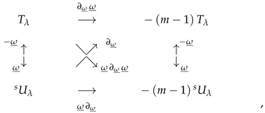
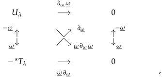
8.4. The Operators ${\partial }_{\underline{\omega }}\underline{\omega }$, $\underline{\omega }{\partial }_{\underline{\omega }}\underline{\omega }$, ${\Delta }^{*}$, and ${\mathbf{Z}}^{*}$

As was stated in Proposition 1, the angular operators ${\partial }_{\underline{\omega }}^2$ and ${\Delta }^{*}$ are Cartesian, and their actions on distributions and on signumdistributions are uniquely determined. As

$${\partial }_{\underline{\omega }}\underline{\omega }=-(m-1)\mathbf{1}+\mathrm{\Gamma },$$

it holds, for all $\lambda \in \mathbb{C}$, that

$${\partial }_{\underline{\omega }}\underline{\omega }{T}_{\lambda }=-(m-1)T_{\lambda },$$

and through the commutative diagram

we obtain, for all $\lambda \in \mathbb{C}$,

• $\underline{\omega }{\partial }_{\underline{\omega }}\underline{\omega }{T}_{\lambda }=-(m-1){}^{s}U_{\lambda }$;
• ${\partial }_{\underline{\omega }}{}^{s}U_{\lambda }=-(m-1)T_{\lambda }$.

These results confirm formula (34).

Similarly, for all $\lambda \in \mathbb{C}$, it holds that

$${\partial }_{\underline{\omega }}\underline{\omega }{U}_{\lambda }=0.$$

Through the commutative diagram

it then follows that, for all $\lambda \in \mathbb{C}$,

• $\underline{\omega }{\partial }_{\underline{\omega }}\underline{\omega }{U}_{\lambda }=0$;
• ${\partial }_{\underline{\omega }}{}^{s}T_{\lambda }=0$.

These results confirm formula (35).

For the actions of the Laplace–Beltrami operator ${\Delta }^{*}=\underline{\omega }{\partial }_{\underline{\omega }}-{\partial }_{\underline{\omega }}^2$ and its signum partner ${\mathbf{Z}}^{*}$, we now find, for all $\lambda \in \mathbb{C}$,

$$\begin{array}{ccc}\hfill {\Delta }^{*}{T}_{\lambda }=0& \mathrm{and}& {\mathbf{Z}}^{*}{}^{s}U_{\lambda }=0;\hfill \end{array}$$

(36)

$$\begin{array}{ccc}\hfill {\Delta }^{*}{U}_{\lambda }=-(m-1)U_{\lambda }& \mathrm{and}& {\mathbf{Z}}^{*}{}^{s}T_{\lambda }=-(m-1){}^{s}T_{\lambda };\hfill \end{array}$$

(37)

$$\begin{array}{ccc}\hfill {\Delta }^{*}{}^{s}T_{\lambda }=0& \mathrm{and}& {\mathbf{Z}}^{*}{U}_{\lambda }=0;\hfill \end{array}$$

(38)

$$\begin{array}{ccc}\hfill {\Delta }^{*}{}^{s}U_{\lambda }=-(m-1){}^{s}U_{\lambda }& \mathrm{and}& {\mathbf{Z}}^{*}{T}_{\lambda }=-(m-1)T_{\lambda }.\hfill \end{array}$$

(39)

8.5. The Operators ${\displaystyle \frac{1}{\underline{x}}}$, ${\displaystyle \frac{1}{r}}$, and ${\displaystyle \frac{1}{r^2}}$

Division of a distribution by $\underline{x}$ is a Cartesian operation that generally leads to an equivalence class of distributions. However, in view of the results in Section 6, we know that under the action of operators ${\displaystyle \frac{1}{\underline{x}}}$ and ${\displaystyle \frac{1}{r}}$, only the distribution $U_{-m+1}$ and the signumdistribution ${}^{s}T_{-m+1}$ will have a non-unique result. The same holds for $U_{-m+1}$, ${}^{s}T_{-m+1}$, $T_{-m+2}$, and ${}^{s}U_{-m+2}$ under the action of operator ${\displaystyle \frac{1}{r^2}}$.

We obtain the following formulæ

$$\begin{array}{|c|}\hline {\displaystyle \frac{1}{r}}{T}_{\lambda }={}^{s}T_{\lambda -1}\\ \hline\end{array}\mathrm{and}\begin{array}{|c|}\hline {\displaystyle \frac{1}{r}}{}^{s}U_{\lambda }=U_{\lambda -1}\\ \hline\end{array},\forall \lambda \in \mathbb{C}$$

and

$$\begin{array}{|c|}\hline {\displaystyle \frac{1}{\underline{x}}}{T}_{\lambda }=-U_{\lambda -1}\\ \hline\end{array}\mathrm{and}\begin{array}{|c|}\hline {\displaystyle \frac{1}{\underline{x}}}{}^{s}U_{\lambda }={}^{s}T_{\lambda -1}\\ \hline\end{array},\forall \lambda \in \mathbb{C}$$

and

$$\begin{array}{|c|}\hline {\displaystyle \frac{1}{r}}{U}_{\lambda }={}^{s}U_{\lambda -1}\\ \hline\end{array}\mathrm{and}\begin{array}{|c|}\hline {\displaystyle \frac{1}{r}}{}^{s}T_{\lambda }=T_{\lambda -1}\\ \hline\end{array},\lambda \ne -m+1$$

and also

$$\begin{array}{|c|}\hline {\displaystyle \frac{1}{\underline{x}}}{U}_{\lambda }=T_{\lambda -1}\\ \hline\end{array}\mathrm{and}\begin{array}{|c|}\hline {\displaystyle \frac{1}{\underline{x}}}{}^{s}T_{\lambda }=-{}^{s}U_{\lambda -1}\\ \hline\end{array},\lambda \ne -m+1.$$

For the exceptional case when $\lambda =-m+1$, we obtain the following results, which are non-unique up to an arbitrary constant c, as

$$\begin{array}{|c|}\hline {\displaystyle \frac{1}{r}}{U}_{-m+1}={}^{s}U_{-m}+\underline{\omega }\delta \left(\underline{x}\right)c\\ \hline\end{array}\mathrm{and}\begin{array}{|c|}\hline {\displaystyle \frac{1}{r}}{}^{s}T_{-m+1}=T_{-m}+\delta \left(\underline{x}\right)c\\ \hline\end{array},$$

and

$$\begin{array}{|c|}\hline {\displaystyle \frac{1}{\underline{x}}}{U}_{-m+1}=T_{-m}+\delta \left(\underline{x}\right)c\\ \hline\end{array}\mathrm{and}\begin{array}{|c|}\hline {\displaystyle \frac{1}{\underline{x}}}{}^{s}T_{-m+1}=-{}^{s}U_{-m}-\underline{\omega }\delta \left(\underline{x}\right)c\\ \hline\end{array}.$$

By iteration, we find formulæfor the division by $r^2$ as follows:

$$\begin{array}{|c|}\hline {\displaystyle \frac{1}{r^2}}{T}_{\lambda }={}^{s}T_{\lambda -2}\\ \hline\end{array}\begin{array}{|c|}\hline {\displaystyle \frac{1}{r^2}}{}^{s}U_{\lambda }={}^{s}U_{\lambda -2}\\ \hline\end{array},\lambda \ne -m+2$$

and

$$\begin{array}{|c|}\hline {\displaystyle \frac{1}{r^2}}{}^{s}T_{\lambda }={}^{s}T_{\lambda -2}\\ \hline\end{array}\begin{array}{|c|}\hline {\displaystyle \frac{1}{r^2}}{U}_{\lambda }={}^{s}U_{\lambda -2}\\ \hline\end{array},\lambda \ne -m+1.$$

For the exceptional case $\lambda =-m+2$, we have

$${\displaystyle \frac{1}{r^2}}{T}_{-m+2}=-{\displaystyle \frac{1}{\underline{x}}}{\displaystyle \frac{1}{\underline{x}}}{T}_{-m+2}={\displaystyle \frac{1}{\underline{x}}}{U}_{-m+1},$$

whence

$$\begin{array}{|c|}\hline {\displaystyle \frac{1}{r^2}}{T}_{-m+2}=T_{-m}+\delta \left(\underline{x}\right)c\\ \hline\end{array}\begin{array}{|c|}\hline {\displaystyle \frac{1}{r^2}}{}^{s}U_{-m+2}={}^{s}U_{-m}+\underline{\omega }\delta \left(\underline{x}\right)c\\ \hline\end{array}.$$

For the exceptional case when $\lambda =-m+1$, we have

$${\displaystyle \frac{1}{r^2}}{U}_{-m+1}=-{\displaystyle \frac{1}{\underline{x}}}{\displaystyle \frac{1}{\underline{x}}}{U}_{-m+1}=-{\displaystyle \frac{1}{\underline{x}}}(T_{-m}+\delta \left(\underline{x}\right)c),$$

whence

$$\begin{array}{|c|}\hline {\displaystyle \frac{1}{r^2}}{}^{s}T_{-m+1}={}^{s}T_{-m-1}-{\displaystyle \frac{1}{m}}{\partial }_r\delta \left(\underline{x}\right)c\\ \hline\end{array}\begin{array}{|c|}\hline {\displaystyle \frac{1}{r^2}}{U}_{-m+1}=U_{-m-1}-{\displaystyle \frac{1}{m}}\underline{\partial }\delta \left(\underline{x}\right)c\\ \hline\end{array}.$$

The action of the operator ${\displaystyle \frac{1}{\underline{x}}}$ components $(-{\displaystyle \frac{x_j}{r^2}}),j=1,\dots ,m$, acting on all $T_{\lambda }$ and $U_{\lambda }$, is uniquely determined, except for $U_{-m+1}$. We readily have

$$\begin{array}{|c|}\hline (-{\displaystyle \frac{x_j}{r^2}})T_{\lambda }=-x_j{T}_{\lambda -2}\\ \hline\end{array}\begin{array}{|c|}\hline (-{\displaystyle \frac{x_j}{r^2}}){}^{s}U_{\lambda }=-x_j{}^{s}U_{\lambda -2}\\ \hline\end{array},\lambda \in \mathbb{C}.$$

Further, for $\lambda \ne -m+1$, we have

$$\begin{array}{|c|}\hline (-{\displaystyle \frac{x_j}{r^2}})U_{\lambda }=-x_j{U}_{\lambda -2}\\ \hline\end{array}\begin{array}{|c|}\hline (-{\displaystyle \frac{x_j}{r^2}}){}^{s}T_{\lambda }=-x_j{}^{s}T_{\lambda -2}\\ \hline\end{array},\lambda \ne -m+1,$$

while for the exceptional case when $\lambda =-m+1$, it holds that

$$(-{\displaystyle \frac{x_j}{r^2}})U_{-m+1}=-x_j(U_{-m-1}-{\displaystyle \frac{1}{m}}\underline{\partial }\delta \left(\underline{x}\right)c),$$

whence

$$\begin{array}{|c|}\hline (-{\displaystyle \frac{x_j}{r^2}})U_{-m+1}=-x_j{U}_{-m-1}+{\displaystyle \frac{1}{m}}{x}_j\underline{\partial }\delta \left(\underline{x}\right)c\\ \hline\end{array},$$

and

$$\begin{array}{|c|}\hline (-{\displaystyle \frac{x_j}{r^2}}){}^{s}T_{-m+1}=-x_j{}^{s}T_{-m-1}-{\omega }_j\delta \left(\underline{x}\right)c\\ \hline\end{array},$$

or

$$\begin{array}{|c|}\hline (-{\displaystyle \frac{x_j}{r^2}})U_{-m+1}=-x_j{U}_{-m-1}-{\displaystyle \frac{1}{m}}\delta \left(\underline{x}\right)c{e}_j\\ \hline\end{array},$$

and

$$\begin{array}{|c|}\hline (-{\displaystyle \frac{x_j}{r^2}}){}^{s}T_{-m+1}=-x_j{}^{s}T_{-m-1}+{\displaystyle \frac{1}{m}}\underline{\omega }\delta \left(\underline{x}\right)c{e}_j\\ \hline\end{array}.$$

8.6. The Operators ${\omega }_j,j=1,\dots ,m$

The multiplication operator ${\omega }_j,j=1,\dots ,m$ is a spherical operator whose actions are uniquely determined (see Definition 4 in Section 5). For all $\lambda \in \mathbb{C}$, it holds that

$${\omega }_j{T}_{\lambda }={\left\{\underline{\omega }{T}_{\lambda }\right\}}_j={{\{}^s{U}_{\lambda }\}}_j=x_j{}^{s}T_{\lambda -1},$$

and, through signum association,

$${\omega }_j{}^{s}U_{\lambda }=x_j{U}_{\lambda -1}.$$

It is verified at once that

$$\underline{\omega }{T}_{\lambda }={\Sigma }_{j=1}^m{e}_j{\omega }_j{T}_{\lambda }={\Sigma }_{j=1}^m{e}_j{x}_j{}^{s}T_{\lambda -1}=\underline{x}{}^{s}T_{\lambda -1}={}^{s}U_{\lambda },$$

and

$$\underline{\omega }{}^{s}U_{\lambda }={\Sigma }_{j=1}^m{e}_j{\omega }_j{}^{s}U_{\lambda }={\Sigma }_{j=1}^m{e}_j{x}_j{U}_{\lambda -1}=\underline{x}{U}_{\lambda -1}=-T_{\lambda }.$$

Similarly, we find that

$${\omega }_j{U}_{\lambda }=\sum _k{\omega }_j{\left\{U_{\lambda }\right\}}_k{e}_k=\sum _k{\omega }_j{x}_k{T}_{\lambda -1}{e}_k=\sum _k{x}_k{x}_j{}^{s}T_{\lambda -2}{e}_k=x_j{}^{s}U_{\lambda -1},$$

and, through signum association,

$${\omega }_j{}^{s}T_{\lambda }=x_j{T}_{\lambda -1}.$$

By iteration, for all $\lambda \in \mathbb{C}$, it follows that

$$\begin{array}{cc}\hfill {\omega }_k{\omega }_j{T}_{\lambda }& =x_j{x}_k{T}_{\lambda -2};\hfill \\ \hfill {\omega }_k{\omega }_j{U}_{\lambda }& =x_j{x}_k{U}_{\lambda -2};\hfill \\ \hfill {\omega }_k{\omega }_j{}^{s}T_{\lambda }& =x_j{x}_k{}^{s}T_{\lambda -2};\hfill \\ \hfill {\omega }_k{\omega }_j{}^{s}U_{\lambda }& =x_j{x}_k{}^{s}U_{\lambda -2}.\hfill \end{array}$$

8.7. The Operators $\underline{\omega }{\partial }_r$, ${\displaystyle \frac{1}{r}}{\partial }_{\underline{\omega }}$, and ${\partial }_r$

As we know how to divide by $\underline{x}$ the distributions $T_{\lambda }$ and $U_{\lambda }$, we are now ready to compute the actions of the radial and angular parts of the Dirac operator through procedures (3) and (4), respectively. Generally, the results of these actions are equivalence classes of distributions. However, we know from Section 6 that we may expect uniquely determined results, except for distribution $U_{-m+1}$ and signumdistribution ${}^{s}T_{-m+1}$.

First, we address the distributions $T_{\lambda }$. For $\lambda \ne -m,-m-2,\dots$, we find that $\left(\underline{\omega }{\partial }_r\right)T_{\lambda }$ is uniquely determined by

$$\left(\underline{\omega }{\partial }_r\right)T_{\lambda }=-\left[{\displaystyle \frac{1}{\underline{x}}}\mathbb{E}{T}_{\lambda }\right]=-\left[{\displaystyle \frac{1}{\underline{x}}}\lambda T_{\lambda }\right]==-{\displaystyle \frac{1}{\underline{x}}}\lambda T_{\lambda }=\lambda U_{\lambda -1}.$$

In view of (7), it follows that

$$\left({\displaystyle \frac{1}{r}}{\partial }_{\underline{\omega }}\right)T_{\lambda }=0,\lambda \ne -m,-m-2,\dots .$$

For the exceptional cases we find that the distributions $\left(\underline{\omega }{\partial }_r\right)T_{-m-2\ell },\ell =0,1,2,\dots$ are uniquely determined by

$$\begin{array}{ccc}\hfill \left(\underline{\omega }{\partial }_r\right)T_{-m-2\ell }& =& -\left[{\displaystyle \frac{1}{\underline{x}}}\mathbb{E}{T}_{-m-2\ell }\right]\hfill \\ & =& -\left[{\displaystyle \frac{1}{\underline{x}}}\left(-(m+2\ell )T_{-m-2\ell }+{(-1)}^{\ell }{\displaystyle \frac{m+2\ell }{C(m,\ell )}}{a}_m{\underline{\partial }}^{2\ell }\delta \left(\underline{x}\right)\right)\right]\hfill \\ & =& -(m+2\ell )U_{-m-2\ell -1}+{(-1)}^{\ell +1}{\displaystyle \frac{1}{C(m,\ell )}}{a}_m{\underline{\partial }}^{2\ell +1}\delta \left(\underline{x}\right).\hfill \end{array}$$

In view of (9), it follows that

$$\left({\displaystyle \frac{1}{r}}{\partial }_{\underline{\omega }}\right)T_{-m-2\ell }=0,,\ell =0,1,2,\dots .$$

In particular, for $\lambda =-m$, we have

$$\begin{array}{ccc}\hfill \left(\underline{\omega }{\partial }_r\right)T_{-m}& =& -\left[{\displaystyle \frac{1}{\underline{x}}}\mathbb{E}{T}_{-m}\right]=-\left[{\displaystyle \frac{1}{\underline{x}}}(-m{T}_{-m}+a_m\delta \left(\underline{x}\right))\right]\hfill \\ & =& (-m)U_{-m-1}-{\displaystyle \frac{1}{m}}{a}_m\underline{\partial }\delta \left(\underline{x}\right)\hfill \end{array}$$

and

$$\left({\displaystyle \frac{1}{r}}{\partial }_{\underline{\omega }}\right)T_{-m}=0,$$

which are in accordance with (11).

Notice that the formula

$$\begin{array}{|c|}\hline \left({\displaystyle \frac{1}{r}}{\partial }_{\underline{\omega }}\right)T_{\lambda }=0\\ \hline\end{array}$$

thus holds for all $\lambda \in \mathbb{C}$.

Through the signum pair of operators $[\underline{\omega }{\partial }_r,\underline{\omega }{\partial }_r]$ and the corresponding commutative diagrams we then obtain the following formulæ.

For $\lambda \ne -m,-m-2,\dots$, the following hold:

• ${\partial }_r{T}_{\lambda }=\lambda {}^{s}T_{\lambda -1}$;
• ${\partial }_r{}^{s}U_{\lambda }=\lambda U_{\lambda -1}$;
• $\left(\underline{\omega }{\partial }_r\right){}^{s}U_{\lambda }=-\lambda {}^{s}T_{\lambda -1}$.

For the exceptional values $\lambda =-m-2\ell ,\ell =0,1,2,\dots$, the following hold:

• ${\partial }_r{T}_{-m-2\ell }=-(m+2\ell ){}^{s}T_{-m-2\ell -1}+{(-1)}^{\ell }{\displaystyle \frac{1}{C(m,\ell )}}{a}_m\underline{\omega }{\underline{\partial }}^{2\ell +1}\delta \left(\underline{x}\right)$;
• ${\partial }_r{}^{s}U_{-m-2\ell }=-(m+2\ell )U_{-m-2\ell -1}+{(-1)}^{\ell +1}{\displaystyle \frac{1}{C(m,\ell )}}{a}_m{\underline{\partial }}^{2\ell +1}\delta \left(\underline{x}\right)$;
• $\left(\underline{\omega }{\partial }_r\right){}^{s}U_{-m-2\ell }=(m+2\ell ){}^{s}T_{-m-2\ell -1}+{(-1)}^{\ell +1}{\displaystyle \frac{1}{C(m,\ell )}}{a}_m\underline{\omega }{\underline{\partial }}^{2\ell +1}\delta \left(\underline{x}\right)$.

In particular, for $\ell =0$, the following hold:

• ${\partial }_r{T}_{-m}=(-m){}^{s}T_{-m-1}-{\displaystyle \frac{1}{m}}{a}_m{\partial }_r\delta \left(\underline{x}\right)$;
• ${\partial }_r{}^{s}U_{-m}=(-m)U_{-m-1}-{\displaystyle \frac{1}{m}}{a}_m\underline{\partial }\delta \left(\underline{x}\right)$;
• $\left(\underline{\omega }{\partial }_r\right){}^{s}U_{-m}=m{}^{s}T_{-m-1}+{\displaystyle \frac{1}{m}}{a}_m{\partial }_r\delta \left(\underline{x}\right)$.

Through the signum pair of operators $[{\displaystyle \frac{1}{r}}{\partial }_{\underline{\omega }},-{\displaystyle \frac{1}{r}}\underline{\omega }{\partial }_{\underline{\omega }}\underline{\omega }]$ and the corresponding commutative diagrams, we obtain, for all $\lambda \in \mathbb{C}$, that

• ${\displaystyle \frac{1}{r}}\mathrm{\Gamma }{T}_{\lambda }=0$;
• ${\displaystyle \frac{1}{r}}\mathrm{\Gamma }{}^{s}U_{\lambda }=(m-1)U_{\lambda -1}$;
• $\begin{array}{|c|}\hline \left({\displaystyle \frac{1}{r}}{\partial }_{\underline{\omega }}\right){}^{s}U_{\lambda }=-(m-1){}^{s}T_{\lambda -1}\\ \hline\end{array}$.

Now, let us turn our attention to the distributions $U_{\lambda }$.

For $\lambda \ne -m+1,-m-1,\dots$, we find the unique expressions

$$\left(\underline{\omega }{\partial }_r\right)U_{\lambda }=-\left[{\displaystyle \frac{1}{\underline{x}}}\mathbb{E}{U}_{\lambda }\right]=-\left[{\displaystyle \frac{1}{\underline{x}}}\lambda U_{\lambda }\right]=-\lambda T_{\lambda -1},$$

and

$$\left({\displaystyle \frac{1}{r}}{\partial }_{\underline{\omega }}\right)U_{\lambda }=-\left[{\displaystyle \frac{1}{\underline{x}}}\mathrm{\Gamma }{U}_{\lambda }\right]=-\left[{\displaystyle \frac{1}{\underline{x}}}(m-1)U_{\lambda }\right]=-(m-1)T_{\lambda -1},$$

which are in accordance with (8).

In the exceptional cases, we find, using (30), for $\ell =1,2,\dots$, the unique expressions

$$\begin{array}{ccc}\hfill \left(\underline{\omega }{\partial }_r\right)U_{-m-2\ell +1}& =& -\left[{\displaystyle \frac{1}{\underline{x}}}\mathbb{E}{U}_{-m-2\ell +1}\right]\hfill \\ & =& -\left[{\displaystyle \frac{1}{\underline{x}}}\left(-(m+2\ell -1)U_{-m-2\ell +1}\right)\right]\hfill \\ & +& {(-1)}^{\ell +1}\left[{\displaystyle \frac{1}{\underline{x}}}{\displaystyle \frac{1}{C(m,\ell -1)}}{a}_m{\underline{\partial }}^{2\ell -1}\delta \left(\underline{x}\right)\right]\hfill \\ & =& (m+2\ell -1)T_{-m-2\ell }+{(-1)}^{\ell +1}{\displaystyle \frac{m+2\ell }{C(m,\ell )}}{a}_m{\underline{\partial }}^{2\ell }\delta \left(\underline{x}\right),\hfill \end{array}$$

and

$$\begin{array}{ccc}\hfill \left({\displaystyle \frac{1}{r}}{\partial }_{\underline{\omega }}\right)U_{-m-2\ell +1}& =& -\left[{\displaystyle \frac{1}{\underline{x}}}\mathrm{\Gamma }{U}_{-m-2\ell +1}\right]\hfill \\ & =& -\left[{\displaystyle \frac{1}{\underline{x}}}(m-1)U_{-m-2\ell +1}\right]\hfill \\ & =& -(m-1)T_{-m-2\ell },\hfill \end{array}$$

which are in accordance with (10).

In the particular case where $\lambda =-m+1$, we find, using (33), the entangled expressions

$$\begin{array}{ccc}\hfill \left(\underline{\omega }{\partial }_r\right)U_{-m+1}& =& -\left[{\displaystyle \frac{1}{\underline{x}}}\mathbb{E}{U}_{-m+1}\right]=-\left[{\displaystyle \frac{1}{\underline{x}}}(-m+1)U_{-m+1}\right]\hfill \\ & =& (m-1)T_{-m}+\delta \left(\underline{x}\right)c_1,\hfill \end{array}$$

(40)

and

$$\begin{array}{ccc}\hfill \left({\displaystyle \frac{1}{r}}{\partial }_{\underline{\omega }}\right)U_{-m+1}& =& -\left[{\displaystyle \frac{1}{\underline{x}}}\mathrm{\Gamma }{U}_{-m+1}\right]=-\left[{\displaystyle \frac{1}{\underline{x}}}(m-1)U_{-m+1}\right]\hfill \\ & =& -(m-1)T_{-m}+\delta \left(\underline{x}\right)c_2,\hfill \end{array}$$

(41)

where, as seen in (12), the arbitrary constants $c_1$ and $c_2$ must satisfy the entanglement condition

$$c_1+c_2=-a_m.$$

(42)

Remark 7.

It should be noted that, in Section 8.8, we fix a particular choice for constants $c_1$ and $c_2$ satisfying (42), in this way defining both $\left(\underline{\omega }{\partial }_r\right)U_{-m+1}$ and $\left({\displaystyle \frac{1}{r}}{\partial }_{\underline{\omega }}\right)U_{-m+1}$.

Through the actions of the operators $\underline{\omega }{\partial }_r$ and ${\displaystyle \frac{1}{r}}{\partial }_{\underline{\omega }}$, it is possible to recover the formulæfor the action of the Laplace operator.

• For $\lambda \ne -m+2,-m,-m-2,\dots$, we have

  $$\begin{array}{cc}\hfill {\left(\underline{\omega }{\partial }_r\right)}^2{T}_{\lambda }& =\left(\underline{\omega }{\partial }_r\right)\left(\lambda U_{\lambda -1}\right)=-\lambda (\lambda -1)T_{\lambda -2}\hfill \\ \hfill \left({\displaystyle \frac{1}{r}}{\partial }_{\underline{\omega }}\right)\left(\underline{\omega }{\partial }_r\right)T_{\lambda }& =\left({\displaystyle \frac{1}{r}}{\partial }_{\underline{\omega }}\right)\left(\lambda U_{\lambda -1}\right)=-\lambda (m-1)T_{\lambda -2}.\hfill \end{array}$$
  Keeping in mind that $\left({\displaystyle \frac{1}{r}}{\partial }_{\underline{\omega }}\right)T_{\lambda }=0$, it is confirmed that

  $$\Delta T_{\lambda }=\lambda (\lambda +m-2)T_{\lambda -2}.$$
• For $\lambda =-m+2$, we have

  $$\begin{array}{cc}\hfill {\left(\underline{\omega }{\partial }_r\right)}^2{T}_{-m+2}& =\left(\underline{\omega }{\partial }_r\right)\left((-m+2)U_{-m+1}\right)\hfill \\ & =-(m-2)((m-1)T_{-m}-a_m\delta \left(\underline{x}\right))\hfill \\ \hfill \left({\displaystyle \frac{1}{r}}{\partial }_{\underline{\omega }}\right)\left(\underline{\omega }{\partial }_r\right)T_{-m+2}& =\left({\displaystyle \frac{1}{r}}{\partial }_{\underline{\omega }}\right)\left((-m+2)U_{-m+1}\right)=(m-2)(m-1)T_{-m},\hfill \end{array}$$

  confirming that

  $$\Delta T_{-m+2}=-(m-2)a_m\delta \left(\underline{x}\right).$$
• For $\lambda =-m-2\ell$, we have

  $${\left(\underline{\omega }{\partial }_r\right)}^2{T}_{-m-2\ell }=\left(\underline{\omega }{\partial }_r\right)(-(m+2\ell )U_{-m-2\ell -1}$$

  $$+{(-1)}^{\ell +1}{\displaystyle \frac{(2\ell +2)(m+2\ell +2)}{C(m,\ell +1)}}{a}_m{\underline{\partial }}^{2\ell +1}\delta \left(\underline{x}\right))$$

  $$\begin{array}{cc}\hfill & =-(m+2\ell )(m+2\ell +1)T_{-m-2\ell -2}\hfill \\ & +{(-1)}^{\ell +1}{\displaystyle \frac{m+2\ell +2}{C(m,\ell +1)}}(2m+4\ell +1)a_m{\underline{\partial }}^{2\ell +2}\delta \left(\underline{x}\right),\hfill \end{array}$$

  and

  $$\left({\displaystyle \frac{1}{r}}{\partial }_{\underline{\omega }}\right)\left(\underline{\omega }{\partial }_r\right)T_{-m-2\ell }=\left({\displaystyle \frac{1}{r}}{\partial }_{\underline{\omega }}\right)(-(m+2\ell )U_{-m-2\ell -1}$$

  $$+{(-1)}^{\ell +1}{\displaystyle \frac{(2\ell +2)(m+2\ell +2)}{C(m,\ell +1)}}{a}_m{\underline{\partial }}^{2\ell +1}\delta \left(\underline{x}\right))$$

  $$=-(m+2\ell )(1-m)T_{-m-2\ell -2}+{(-1)}^{\ell +1}{\displaystyle \frac{m+2\ell +2}{C(m,\ell +1)}}(1-m)a_m{\underline{\partial }}^{2\ell +2}\delta \left(\underline{x}\right),$$

  confirming that

  $$\begin{array}{cc}\hfill \Delta T_{-m-2\ell }& =(m+2\ell )(2\ell +2)T_{-m-2\ell -2}\hfill \\ & +{(-1)}^{\ell }{\displaystyle \frac{(m+4\ell +2)(m+2\ell +2)}{C(m,\ell +1)}}{a}_m{\underline{\partial }}^{2\ell +2}\delta \left(\underline{x}\right).\hfill \end{array}$$
• For $\lambda \ne -m+1,-m-1,-m-3,\dots$, we have

  $$\begin{array}{cc}\hfill {\left(\underline{\omega }{\partial }_r\right)}^2{U}_{\lambda }& =\left(\underline{\omega }{\partial }_r\right)(-\lambda T_{\lambda -1})=-\lambda (\lambda -1)U_{\lambda -2}\hfill \\ \hfill \left({\displaystyle \frac{1}{r}}{\partial }_{\underline{\omega }}\right)\left(\underline{\omega }{\partial }_r\right)U_{\lambda }& =\left({\displaystyle \frac{1}{r}}{\partial }_{\underline{\omega }}\right)(-\lambda T_{\lambda -1})=0\hfill \\ \hfill \left(\underline{\omega }{\partial }_r\right)\left({\displaystyle \frac{1}{r}}{\partial }_{\underline{\omega }}\right)U_{\lambda }& =\left(\underline{\omega }{\partial }_r\right)(-(m-1)T_{\lambda -1})=-(m-1)(\lambda -1)U_{\lambda -2}\hfill \\ \hfill \left({\displaystyle \frac{1}{r}}{\partial }_{\underline{\omega }}\right)\left({\displaystyle \frac{1}{r}}{\partial }_{\underline{\omega }}\right)U_{\lambda }& =\left({\displaystyle \frac{1}{r}}{\partial }_{\underline{\omega }}\right)(-(m-1)T_{\lambda -1})=0,\hfill \end{array}$$

  confirming that

  $$\Delta U_{\lambda }=(\lambda -1)(\lambda +m-1)U_{\lambda -2}.$$
• For $\lambda =-m+1$, we have

  $$\begin{array}{cc}\hfill {\left(\underline{\omega }{\partial }_r\right)}^2{U}_{-m+1}& =\left(\underline{\omega }{\partial }_r\right)((m-1)T_{-m}-a_m\delta \left(\underline{x}\right))\hfill \\ \hfill & =-(m-1)m{U}_{-m-1}-{\displaystyle \frac{2m-1}{m}}{a}_m\underline{\partial }\delta \left(\underline{x}\right)\hfill \\ \hfill \left({\displaystyle \frac{1}{r}}{\partial }_{\underline{\omega }}\right)\left(\underline{\omega }{\partial }_r\right)U_{-m+1}& =\left({\displaystyle \frac{1}{r}}{\partial }_{\underline{\omega }}\right)((m-1)T_{-m}-a_m\delta \left(\underline{x}\right))=0\hfill \\ \hfill \left(\underline{\omega }{\partial }_r\right)\left({\displaystyle \frac{1}{r}}{\partial }_{\underline{\omega }}\right)U_{-m+1}& =\left(\underline{\omega }{\partial }_r\right)(-(m-1)T_{-m})\hfill \\ \hfill & =(m-1)m{U}_{-m-1}+{\displaystyle \frac{m-1}{m}}{a}_m\underline{\partial }\delta \left(\underline{x}\right)\hfill \\ \hfill \left({\displaystyle \frac{1}{r}}{\partial }_{\underline{\omega }}\right)\left({\displaystyle \frac{1}{r}}{\partial }_{\underline{\omega }}\right)U_{-m+1}& =\left({\displaystyle \frac{1}{r}}{\partial }_{\underline{\omega }}\right)(-(m-1)T_{-m})=0,\hfill \end{array}$$

  confirming that

  $$\Delta U_{-m+1}=a_m\underline{\partial }\delta \left(\underline{x}\right).$$
• For $\lambda =-m-2\ell +1$, we have

  $$\begin{array}{cc}\hfill {\left(\underline{\omega }{\partial }_r\right)}^2{U}_{-m+1}& =-(m+2\ell -1)(m+2\ell )U_{-m-2\ell -1}\hfill \\ \hfill & +{(-1)}^{\ell +1}{\displaystyle \frac{2m+4\ell -1}{C(m,\ell )}}{a}_m{\underline{\partial }}^{2\ell +1}\hfill \\ \hfill \left({\displaystyle \frac{1}{r}}{\partial }_{\underline{\omega }}\right)\left(\underline{\omega }{\partial }_r\right)U_{-m+1}& =0\hfill \\ \hfill \left(\underline{\omega }{\partial }_r\right)\left({\displaystyle \frac{1}{r}}{\partial }_{\underline{\omega }}\right)U_{-m+1}& =(m+2\ell )(m-1)U_{-m-2\ell -1}\hfill \\ \hfill & -{(-1)}^{\ell +1}{\displaystyle \frac{m-1}{C(m,\ell )}}{a}_m{\underline{\partial }}^{2\ell +1}\delta \left(\underline{x}\right)\hfill \\ \hfill \left({\displaystyle \frac{1}{r}}{\partial }_{\underline{\omega }}\right)\left({\displaystyle \frac{1}{r}}{\partial }_{\underline{\omega }}\right)U_{-m+1}& =0,\hfill \end{array}$$

  confirming that

  $$\Delta U_{-m-2\ell +1}=(m+2\ell )(2\ell )U_{-m-2\ell -1}+{(-1)}^{\ell }{a}_m{\displaystyle \frac{m+4\ell }{C(m,\ell )}}{\underline{\partial }}^{2\ell +1}\delta \left(\underline{x}\right).$$

Through the signum pair of operators $[\underline{\omega }{\partial }_r,\underline{\omega }{\partial }_r]$ and the corresponding commutative diagrams, we obtain the following formulæ.

For $\lambda \ne -m+1,-m-1,\dots$, the following hold:

• ${\partial }_r{U}_{\lambda }=\lambda {}^{s}U_{\lambda -1}$;
• ${\partial }_r{}^{s}T_{\lambda }=\lambda T_{\lambda -1}$;
• $\left(\underline{\omega }{\partial }_r\right){}^{s}T_{\lambda }=\lambda {}^{s}U_{\lambda -1}$.

For the exceptional values $\lambda =-m-2\ell +1,\ell =1,2,\dots$, the following hold:

• ${\partial }_r{U}_{-m-2\ell +1}=-(m+2\ell -1){}^{s}U_{-m-2\ell }+{(-1)}^{\ell }{\displaystyle \frac{m+2\ell }{C(m,\ell )}}{a}_m\underline{\omega }{\underline{\partial }}^{2\ell }\delta \left(\underline{x}\right)$;
• ${\partial }_r{}^{s}T_{-m-2\ell +1}=-(m+2\ell -1)T_{-m-2\ell }+{(-1)}^{\ell }{\displaystyle \frac{m+2\ell }{C(m,\ell )}}{a}_m{\underline{\partial }}^{2\ell }\delta \left(\underline{x}\right)$;
• $\left(\underline{\omega }{\partial }_r\right){}^{s}T_{-m-2\ell +1}=-(m+2\ell -1){}^{s}U_{-m-2\ell }+{(-1)}^{\ell }{\displaystyle \frac{m+2\ell }{C(m,\ell )}}{a}_m\underline{\omega }{\underline{\partial }}^{2\ell }\delta \left(\underline{x}\right)$.

On the other hand, for $\ell =0$, the following hold:

• ${\partial }_r{U}_{-m+1}=-(m-1){}^{s}U_{-m}-\underline{\omega }\delta \left(\underline{x}\right)c_1$;
• ${\partial }_r{}^{s}T_{-m+1}=-(m-1)T_{-m}-\delta \left(\underline{x}\right)c_1$;
• $\left(\underline{\omega }{\partial }_r\right){}^{s}T_{-m+1}=-(m-1){}^{s}U_{-m}-\underline{\omega }\delta \left(\underline{x}\right)c_1$.

Through the signum pair of operators $[{\displaystyle \frac{1}{r}}{\partial }_{\underline{\omega }},-{\displaystyle \frac{1}{r}}\underline{\omega }{\partial }_{\underline{\omega }}\underline{\omega }]$ and the corresponding commutative diagrams, we obtain the following formulæ.

For $\lambda \ne -m+1,-m-1,\dots$, the following hold:

• $(-{\displaystyle \frac{1}{r}}\mathrm{\Gamma }+(m-1){\displaystyle \frac{1}{r}}){}^{s}T_{\lambda }=(m-1)T_{\lambda -1}$;
• ${\displaystyle \frac{1}{r}}\mathrm{\Gamma }{U}_{\lambda }=(m-1){}^{s}U_{\lambda -1}$;
• $(-{\displaystyle \frac{1}{r}}{\partial }_{\underline{\omega }}+(m-1){\displaystyle \frac{1}{r}}\underline{\omega }){}^{s}T_{\lambda }=(m-1){}^{s}U_{\lambda -1}$.

Equivalently, the following hold:

• ${\displaystyle \frac{1}{r}}{}^{s}T_{\lambda }=T_{\lambda -1}$;
• ${\displaystyle \frac{1}{r}}\mathrm{\Gamma }{U}_{\lambda }=(m-1){}^{s}U_{\lambda -1}$;
• ${\displaystyle \frac{1}{r}}{\partial }_{\underline{\omega }}{}^{s}T_{\lambda }=0$.

For the exceptional values $\lambda =-m-2\ell +1,\ell =1,2,\dots$, the following hold:

• $(-{\displaystyle \frac{1}{r}}\mathrm{\Gamma }+(m-1){\displaystyle \frac{1}{r}}){}^{s}T_{-m-2\ell +1}=(m-1)T_{m-2\ell }$;
• ${\displaystyle \frac{1}{r}}\mathrm{\Gamma }{U}_{-m-2\ell +1}=(m-1){}^{s}U_{m-2\ell }$;
• $(-{\displaystyle \frac{1}{r}}{\partial }_{\underline{\omega }}+(m-1){\displaystyle \frac{1}{r}}\underline{\omega }){}^{s}T_{-m-2\ell +1}=(m-1){}^{s}U_{m-2\ell }$.

Equivalently, the following hold:

• ${\displaystyle \frac{1}{r}}{}^{s}T_{-m-2\ell +1}=T_{m-2\ell }$
• ${\displaystyle \frac{1}{r}}\mathrm{\Gamma }{U}_{-m-2\ell +1}=(m-1){}^{s}U_{m-2\ell }$
• ${\displaystyle \frac{1}{r}}{\partial }_{\underline{\omega }}{}^{s}T_{-m-2\ell +1}=0$.

For the exceptional value $\lambda =-m+1$, the following hold:

• $(-{\displaystyle \frac{1}{r}}\mathrm{\Gamma }+(m-1){\displaystyle \frac{1}{r}}){}^{s}T_{-m+1}=(m-1)T_{-m}-\delta \left(\underline{x}\right)c_2$;
• ${\displaystyle \frac{1}{r}}\mathrm{\Gamma }{U}_{-m+1}=(m-1){}^{s}U_{-m}+\underline{\omega }\delta \left(\underline{x}\right)c_2$;
• $(-{\displaystyle \frac{1}{r}}{\partial }_{\underline{\omega }}+(m-1){\displaystyle \frac{1}{r}}\underline{\omega }){}^{s}T_{-m+1}=(m-1){}^{s}U_{-m}-\underline{\omega }\delta \left(\underline{x}\right)c_2$.

Equivalently, the following hold:

• $(m-1){\displaystyle \frac{1}{r}}{}^{s}T_{-m+1}=(m-1)T_{-m}-\delta \left(\underline{x}\right)c_2$;
• ${\displaystyle \frac{1}{r}}\mathrm{\Gamma }{U}_{-m+1}=(m-1){}^{s}U_{-m}+\underline{\omega }\delta \left(\underline{x}\right)c_2$;
• $\left({\displaystyle \frac{1}{r}}{\partial }_{\underline{\omega }}\right){}^{s}T_{-m+1}=0$.

Note that the formula

$$\begin{array}{|c|}\hline \left({\displaystyle \frac{1}{r}}{\partial }_{\underline{\omega }}\right){}^{s}T_{\lambda }=0\\ \hline\end{array}$$

is valid for all $\lambda \in \mathbb{C}$.

As expected, $U_{-m+1}$ is the only distribution in the two families of distributions $T_{\lambda }$ and $U_{\lambda }$, $\lambda \in \mathbb{C}$, for which the actions of the operators ${\underline{\partial }}_{rad}$ and ${\underline{\partial }}_{ang}$ are not uniquely determined, and a similar observation holds for the signumdistribution ${}^{s}T_{-m+1}$. Nothing prevents us from defining these actions by selecting specific values for the arbitrary constants involved. However, to avoid possible inconsistencies, we will, for the moment, not do so and keep the constants $c_1$ and $c_2$ arbitrary but constrained by the entanglement condition (42), viz., $c_1+c_2=-a_m$. This is made possible by the fact that ${\displaystyle \frac{1}{\underline{x}}}{U}_{-m+1}$ is expressed as an equivalence class of distributions, viz.,

$${\displaystyle \frac{1}{\underline{x}}}{U}_{-m+1}=T_{-m}+\delta \left(\underline{x}\right)c,$$

which is necessary, because fixing here and now a particular value for this arbitrary constant c would lead to the impossible result $\underline{\partial }{U}_{-m+1}=0$.

8.8. The Operators $\underline{D}$ and $\mathbf{Z}$

Combining the results obtained in Section 8.7 for the actions of the radial and angular parts of the Dirac operator, we obtain the action of operator $\underline{D}$ on the distributions $T_{\lambda }$ and $U_{\lambda }$ and of the Dirac operator $\underline{\partial }$ on the signumdistributions ${}^{s}T_{\lambda }$ and ${}^{s}U_{\lambda }$. These results should match with each other through the signum pair of operators $[\underline{D},\underline{\partial }]$. We expect $U_{-m+1}$ to be the only distribution for which the $\underline{D}$ action is not uniquely determined and the same for the signumdistribution ${}^{s}T_{-m+1}$ with respect to the $\underline{\partial }$ action. An overview of the results is now given, recalling, for completeness, some formulæalready obtained in the preceding subsections.

First, we consider the case of the distributions $T_{\lambda }$ and the associated signumdistributions ${}^{s}U_{\lambda }$.

For $\begin{array}{|c|}\hline \lambda \ne -m,-m-2,\dots \\ \hline\end{array}$, it holds that

$$\begin{array}{ccc}\hfill \left(\underline{\omega }{\partial }_r\right)T_{\lambda }& =& \lambda U_{\lambda -1}\hfill \end{array}$$

(43)

$$\begin{array}{ccc}\hfill \left({\displaystyle \frac{1}{r}}{\partial }_{\underline{\omega }}\right)T_{\lambda }& =& 0\hfill \end{array}$$

(44)

$$\begin{array}{ccc}\hfill \underline{\partial }{T}_{\lambda }& =& \lambda U_{\lambda -1}\hfill \end{array}$$

(45)

$$\begin{array}{ccc}\hfill \underline{D}{T}_{\lambda }& =& (\lambda +m-1)U_{\lambda -1},\hfill \end{array}$$

(46)

and

$$\begin{array}{ccc}\hfill \left(\underline{\omega }{\partial }_r\right){}^{s}U_{\lambda }& =& -\lambda {}^{s}T_{\lambda -1}\hfill \end{array}$$

(47)

$$\begin{array}{ccc}\hfill \left({\displaystyle \frac{1}{r}}{\partial }_{\underline{\omega }}\right){}^{s}U_{\lambda }& =& -(m-1){}^{s}T_{\lambda -1}\hfill \end{array}$$

(48)

$$\begin{array}{ccc}\hfill \underline{D}{}^{s}U_{\lambda }& =& -\lambda {}^{s}T_{\lambda -1}\hfill \end{array}$$

(49)

$$\begin{array}{ccc}\hfill \underline{\partial }{}^{s}U_{\lambda }& =& -(\lambda +m-1){}^{s}T_{\lambda -1}.\hfill \end{array}$$

(50)

For $\begin{array}{|c|}\hline \lambda =-m\\ \hline\end{array}$, it holds that

$$\begin{array}{ccc}\hfill \left(\underline{\omega }{\partial }_r\right)T_{-m}& =& -m{U}_{-m-1}-{\displaystyle \frac{1}{m}}{a}_m\underline{\partial }\delta \left(\underline{x}\right)\hfill \end{array}$$

(51)

$$\begin{array}{ccc}\hfill \left({\displaystyle \frac{1}{r}}{\partial }_{\underline{\omega }}\right)T_{-m}& =& 0\hfill \end{array}$$

(52)

$$\begin{array}{ccc}\hfill \underline{\partial }{T}_{-m}& =& -m{U}_{-m-1}-{\displaystyle \frac{1}{m}}{a}_m\underline{\partial }\delta \left(\underline{x}\right)\hfill \end{array}$$

(53)

$$\begin{array}{ccc}\hfill \underline{D}{T}_{-m}& =& -U_{-m-1}-{\displaystyle \frac{1}{m}}{a}_m\underline{\partial }\delta \left(\underline{x}\right),\hfill \end{array}$$

(54)

and

$$\begin{array}{ccc}\hfill \left(\underline{\omega }{\partial }_r\right){}^{s}U_{-m}& =& m{}^{s}T_{-m-1}+{\displaystyle \frac{1}{m}}{a}_m{\partial }_r\delta \left(\underline{x}\right)\hfill \end{array}$$

(55)

$$\begin{array}{ccc}\hfill \left({\displaystyle \frac{1}{r}}{\partial }_{\underline{\omega }}\right){}^{s}U_{-m}& =& -(m-1){}^{s}T_{-m-1}\hfill \end{array}$$

(56)

$$\begin{array}{ccc}\hfill \underline{D}{}^{s}U_{-m}& =& m{}^{s}T_{-m-1}+{\displaystyle \frac{1}{m}}{a}_m{\partial }_r\delta \left(\underline{x}\right)\hfill \end{array}$$

(57)

$$\begin{array}{ccc}\hfill \underline{\partial }{}^{s}U_{-m}& =& {}^{s}T_{-m-1}+{\displaystyle \frac{1}{m}}{a}_m{\partial }_r\delta \left(\underline{x}\right).\hfill \end{array}$$

(58)

More generally, for $\begin{array}{|c|}\hline \lambda =-m-2\ell \\ \hline\end{array},\ell =0,1,2,\dots$, it holds that

$$\begin{array}{ccc}\hfill \left(\underline{\omega }{\partial }_r\right)T_{-m-2\ell }& =& -(m+2\ell )U_{-m-2\ell -1}+{(-1)}^{\ell +1}{\displaystyle \frac{1}{C(m,\ell )}}{a}_m{\underline{\partial }}^{2\ell +1}\delta \left(\underline{x}\right)\hfill \end{array}$$

(59)

$$\begin{array}{ccc}\hfill \left({\displaystyle \frac{1}{r}}{\partial }_{\underline{\omega }}\right)T_{-m-2\ell }& =& 0\hfill \end{array}$$

(60)

$$\begin{array}{ccc}\hfill \underline{\partial }{T}_{-m-2\ell }& =& -(m+2\ell )U_{-m-2\ell -1}+{(-1)}^{\ell +1}{\displaystyle \frac{1}{C(m,\ell )}}{a}_m{\underline{\partial }}^{2\ell +1}\delta \left(\underline{x}\right)\hfill \end{array}$$

(61)

$$\begin{array}{ccc}\hfill \underline{D}{T}_{-m-2\ell }& =& -(2\ell +1)U_{-m-2\ell -1}+{(-1)}^{\ell +1}{\displaystyle \frac{1}{C(m,\ell )}}{a}_m{\underline{\partial }}^{2\ell +1}\delta \left(\underline{x}\right)\hfill \end{array}$$

(62)

and

$$\begin{array}{ccc}\hfill \left(\underline{\omega }{\partial }_r\right){}^{s}U_{-m-2\ell }& =& (m+2\ell ){}^{s}T_{-m-2\ell -1}+{(-1)}^{\ell +1}{\displaystyle \frac{1}{C(m,\ell )}}{a}_m\underline{\omega }{\underline{\partial }}^{2\ell +1}\delta \left(\underline{x}\right)\hfill \end{array}$$

(63)

$$\begin{array}{ccc}\hfill \left({\displaystyle \frac{1}{r}}{\partial }_{\underline{\omega }}\right){}^{s}U_{-m-2\ell }& =& -(m-1){}^{s}T_{-m-2\ell -1}\hfill \end{array}$$

(64)

$$\begin{array}{ccc}\hfill \underline{D}{}^{s}U_{-m-2\ell }& =& (m+2\ell ){}^{s}T_{-m-2\ell -1}+{(-1)}^{\ell +1}{\displaystyle \frac{1}{C(m,\ell )}}{a}_m\underline{\omega }{\underline{\partial }}^{2\ell +1}\delta \left(\underline{x}\right)\hfill \end{array}$$

(65)

$$\begin{array}{ccc}\hfill \underline{\partial }{}^{s}U_{-m-2\ell }& =& (2\ell +1){}^{s}T_{-m-2\ell -1}+{(-1)}^{\ell +1}{\displaystyle \frac{1}{C(m,\ell )}}{a}_m\underline{\omega }{\underline{\partial }}^{2\ell +1}\delta \left(\underline{x}\right).\hfill \end{array}$$

(66)

Now, we treat the case of the distributions $U_{\lambda }$ and the associated signumdistributions ${}^{s}T_{\lambda }$.

For $\begin{array}{|c|}\hline \lambda \ne -m+1,-m-1,\dots \\ \hline\end{array}$, it holds that

$$\begin{array}{ccc}\hfill \left(\underline{\omega }{\partial }_r\right)U_{\lambda }& =& -\lambda T_{\lambda -1}\hfill \end{array}$$

(67)

$$\begin{array}{ccc}\hfill \left({\displaystyle \frac{1}{r}}{\partial }_{\underline{\omega }}\right)U_{\lambda }& =& -(m-1)T_{\lambda -1}\hfill \end{array}$$

(68)

$$\begin{array}{ccc}\hfill \underline{\partial }{U}_{\lambda }& =& -(\lambda +m-1)T_{\lambda -1}\hfill \end{array}$$

(69)

$$\begin{array}{ccc}\hfill \underline{D}{U}_{\lambda }& =& -\lambda T_{\lambda -1},\hfill \end{array}$$

(70)

and

$$\begin{array}{ccc}\hfill \left(\underline{\omega }{\partial }_r\right){}^{s}T_{\lambda }& =& \lambda {}^{s}U_{\lambda -1}\hfill \end{array}$$

(71)

$$\begin{array}{ccc}\hfill \left({\displaystyle \frac{1}{r}}{\partial }_{\underline{\omega }}\right){}^{s}T_{\lambda }& =& 0\hfill \end{array}$$

(72)

$$\begin{array}{ccc}\hfill \underline{D}{}^{s}T_{\lambda }& =& (\lambda +m-1){}^{s}U_{\lambda -1}\hfill \end{array}$$

(73)

$$\begin{array}{ccc}\hfill \underline{\partial }{}^{s}T_{\lambda }& =& \lambda {}^{s}U_{\lambda -1}.\hfill \end{array}$$

(74)

For $\begin{array}{|c|}\hline \lambda =-m-2\ell +1\\ \hline\end{array},\ell =1,2,\dots$, it holds that

$$\begin{array}{ccc}\hfill \left(\underline{\omega }{\partial }_r\right)U_{-m-2\ell +1}& =& (m+2\ell -1)T_{-m-2\ell }+{(-1)}^{\ell +1}{\displaystyle \frac{m+2\ell }{C(m,\ell )}}{a}_m{\underline{\partial }}^{2\ell }\delta \left(\underline{x}\right)\hfill \end{array}$$

(75)

$$\begin{array}{ccc}\hfill \left({\displaystyle \frac{1}{r}}{\partial }_{\underline{\omega }}\right)U_{-m-2\ell +1}& =& -(m-1)T_{-m-2\ell }\hfill \end{array}$$

(76)

$$\begin{array}{ccc}\hfill \underline{\partial }{U}_{-m-2\ell +1}& =& (2\ell )T_{-m-2\ell }+{(-1)}^{\ell +1}{\displaystyle \frac{m+2\ell }{C(m,\ell )}}{a}_m{\underline{\partial }}^{2\ell }\delta \left(\underline{x}\right)\hfill \end{array}$$

(77)

$$\begin{array}{ccc}\hfill \underline{D}{U}_{-m-2\ell +1}& =& (m+2\ell -1)T_{-m-2\ell }+{(-1)}^{\ell +1}{\displaystyle \frac{m+2\ell }{C(m,\ell )}}{a}_m{\underline{\partial }}^{2\ell }\delta \left(\underline{x}\right),\hfill \end{array}$$

(78)

and

$$\begin{array}{ccc}\hfill \left(\underline{\omega }{\partial }_r\right){}^{s}T_{-m-2\ell +1}& =& -(m+2\ell -1){}^{s}U_{-m-2\ell }+{(-1)}^{\ell }{\displaystyle \frac{m+2\ell }{C(m,\ell )}}{a}_m\underline{\omega }{\underline{\partial }}^{2\ell }\delta \left(\underline{x}\right)\hfill \end{array}$$

(79)

$$\begin{array}{ccc}\hfill \left({\displaystyle \frac{1}{r}}{\partial }_{\underline{\omega }}\right){}^{s}T_{-m-2\ell +1}& =& 0\hfill \end{array}$$

(80)

$$\begin{array}{ccc}\hfill \underline{D}{}^{s}T_{-m-2\ell +1}& =& -(2\ell ){}^{s}U_{-m-2\ell }+{(-1)}^{\ell }{\displaystyle \frac{m+2\ell }{C(m,\ell )}}{a}_m\underline{\omega }{\underline{\partial }}^{2\ell }\delta \left(\underline{x}\right)\hfill \end{array}$$

(81)

$$\begin{array}{ccc}\hfill \underline{\partial }{}^{s}T_{-m-2\ell +1}& =& -(m+2\ell -1){}^{s}U_{-m-2\ell }+{(-1)}^{\ell }{\displaystyle \frac{m+2\ell }{C(m,\ell )}}{a}_m\underline{\omega }{\underline{\partial }}^{2\ell }\delta \left(\underline{x}\right).\hfill \end{array}$$

(82)

For the exceptional case $\begin{array}{|c|}\hline \lambda =-m+1\\ \hline\end{array}$, we find that

$$\begin{array}{ccc}\hfill \left(\underline{\omega }{\partial }_r\right)U_{-m+1}& =& (m-1)T_{-m}+\delta \left(\underline{x}\right)c_1\hfill \\ \hfill \left({\displaystyle \frac{1}{r}}{\partial }_{\underline{\omega }}\right)U_{-m+1}& =& -(m-1)T_{-m}+\delta \left(\underline{x}\right)c_2\hfill \\ \hfill \underline{\partial }{U}_{-m+1}& =& -a_m\delta \left(\underline{x}\right)\hfill \\ \hfill \underline{D}{U}_{-m+1}& =& (m-1)T_{-m}+\delta \left(\underline{x}\right)c^{*},\hfill \end{array}$$

and

$$\begin{array}{ccc}\hfill \left(\underline{\omega }{\partial }_r\right){}^{s}T_{-m+1}& =& -(m-1){}^{s}U_{-m}-\underline{\omega }\delta \left(\underline{x}\right)c_1\hfill \\ \hfill \left({\displaystyle \frac{1}{r}}{\partial }_{\underline{\omega }}\right){}^{s}T_{-m+1}& =& 0\hfill \\ \hfill \underline{D}{}^{s}T_{-m+1}& =& \underline{\omega }\delta \left(\underline{x}\right)a_m\hfill \\ \hfill \underline{\partial }{}^{s}T_{-m+1}& =& -(m-1){}^{s}U_{-m}-\underline{\omega }\delta \left(\underline{x}\right)c^{*}.\hfill \end{array}$$

Apparently, the constant $c^{*}$ may be chosen freely, whereas constants $c_1$ and $c_2$ must satisfy the entanglement condition (42), which reads as

$$c_1+c_2=-a_m.$$

We now fix these arbitrary constants ourselves, which means that we define $\left(\underline{\omega }{\partial }_r\right)U_{-m+1}$, $\left({\displaystyle \frac{1}{r}}{\partial }_{\underline{\omega }}\right)U_{-m+1}$, and $\underline{D}{U}_{-m+1}$. Quite naturally, we have to be very cautious and constantly monitor the concistency. We made the following choices:

$$c^{*}=c_1=-a_m,c_2=0.$$

Are there any arguments for this particular choice? Concerning the choice of $c^{*}$, one can see that, for general $\lambda$, the expressions for $\left(\underline{\omega }{\partial }_r\right)U_{\lambda }$ and $\underline{D}{U}_{\lambda }$ coincide, inspiring the choice $c^{*}=c_1$. Next, putting $\ell =0$ in the expression for $\left(\underline{\omega }{\partial }_r\right)U_{-m-2\ell +1}$ results in

$$(m-1)T_{-m}-a_m\delta \left(\underline{x}\right),$$

which can then serve as the definition for $\left(\underline{\omega }{\partial }_r\right)U_{-m+1}$, making $c_1=-a_m$ and $c_2=0$. Hence, we have the following definition.

Definition 12.

We define

$$\begin{array}{ccc}\hfill \left(\underline{\omega }{\partial }_r\right)U_{-m+1}& =& (m-1)T_{-m}-a_m\delta \left(\underline{x}\right)\hfill \end{array}$$

(83)

$$\begin{array}{ccc}\hfill \left({\displaystyle \frac{1}{r}}{\partial }_{\underline{\omega }}\right)U_{-m+1}& =& -(m-1)T_{-m}\hfill \end{array}$$

(84)

$$\begin{array}{ccc}\hfill \underline{\partial }{U}_{-m+1}& =& -a_m\delta \left(\underline{x}\right)\hfill \end{array}$$

(85)

$$\begin{array}{ccc}\hfill \underline{D}{U}_{-m+1}& =& (m-1)T_{-m}-a_m\delta \left(\underline{x}\right),\hfill \end{array}$$

(86)

and

$$\begin{array}{ccc}\hfill \left(\underline{\omega }{\partial }_r\right){}^{s}T_{-m+1}& =& -(m-1){}^{s}U_{-m}+a_m\underline{\omega }\delta \left(\underline{x}\right)\hfill \end{array}$$

(87)

$$\begin{array}{ccc}\hfill \left({\displaystyle \frac{1}{r}}{\partial }_{\underline{\omega }}\right){}^{s}T_{-m+1}& =& 0\hfill \end{array}$$

(88)

$$\begin{array}{ccc}\hfill \underline{D}{}^{s}T_{-m+1}& =& a_m\underline{\omega }\delta \left(\underline{x}\right)\hfill \end{array}$$

(89)

$$\begin{array}{ccc}\hfill \underline{\partial }{}^{s}T_{-m+1}& =& -(m-1){}^{s}U_{-m}+a_m\underline{\omega }\delta \left(\underline{x}\right).\hfill \end{array}$$

(90)

It should be noted that formula (84) matches the corresponding formula for all other values of parameter $\lambda$, that is,

$$\left({\displaystyle \frac{1}{r}}{\partial }_{\underline{\omega }}\right)U_{\lambda }=-(m-1)T_{\lambda -1}.$$

The iteration of operators $\underline{\partial }$ and $\underline{D}$ yields the following formulæinvolving Laplace and $\mathbf{Z}$ operators. These results should match each other pairwise through the signum pairs of operators $(\Delta ,\mathbf{Z})$ and $[\mathbf{Z},\Delta ]$. Based on the results in Section 6, we expect the distributions $T_{-m+2}$ and $U_{-m+1}$ to have non-unique results under the action of operator $\mathbf{Z}$. The same holds for the signumdistributions ${}^{s}U_{-m+2}$ and ${}^{s}T_{-m+1}$ under the action of the Laplace operator $\Delta$.

First, we consider the case of the distributions $T_{\lambda }$ and the associated signumdistributions ${}^{s}U_{\lambda }$.

For $\begin{array}{|c|}\hline \lambda \ne -m+2,-m,-m-2,\dots \\ \hline\end{array}$, we already found formulæ (13) and (20), viz.

$$\begin{array}{ccc}\hfill \Delta T_{\lambda }& =& \lambda (\lambda +m-2)T_{\lambda -2}\hfill \\ \hfill \mathbf{Z}{}^{s}U_{\lambda }& =& \lambda (\lambda +m-2){}^{s}U_{\lambda -2},\hfill \end{array}$$

and now, it also holds that

$$\begin{array}{ccc}\hfill \mathbf{Z}{T}_{\lambda }& =& (\lambda -1)(\lambda +m-1)T_{\lambda -2}\hfill \end{array}$$

(91)

$$\begin{array}{ccc}\hfill \Delta {}^{s}U_{\lambda }& =& (\lambda -1)(\lambda +m-1){}^{s}U_{\lambda -2}.\hfill \end{array}$$

(92)

For $\begin{array}{|c|}\hline \lambda =-m+2\\ \hline\end{array}$, we already found formulæ (19) and (26), viz.

$$\begin{array}{ccc}\hfill \Delta T_{-m+2}& =& -(m-2)a_m\delta \left(\underline{x}\right)\hfill \\ \hfill \mathbf{Z}{}^{s}U_{-m+2}& =& -(m-2)a_m\underline{\omega }\delta \left(\underline{x}\right),\hfill \end{array}$$

and now, it also holds that

$$\begin{array}{ccc}\hfill \mathbf{Z}{T}_{-m+2}& =& -(m-1)T_{-m}+a_m\delta \left(\underline{x}\right)\hfill \end{array}$$

(93)

$$\begin{array}{ccc}\hfill \Delta {}^{s}U_{-m+2}& =& -(m-1){}^{s}U_{-m}+a_m\underline{\omega }\delta \left(\underline{x}\right).\hfill \end{array}$$

(94)

For $\begin{array}{|c|}\hline \lambda =-m\\ \hline\end{array}$, we already found formulæ (17) and (24), viz.

$$\begin{array}{ccc}\hfill \Delta T_{-m}& =& 2m{T}_{-m-2}+({\displaystyle \frac{1}{2}}+{\displaystyle \frac{1}{m}})a_m{\underline{\partial }}^2\delta \left(\underline{x}\right)\hfill \\ \hfill \mathbf{Z}{}^{s}U_{-m}& =& 2m{}^{s}U_{-m-2}+({\displaystyle \frac{1}{2}}+{\displaystyle \frac{1}{m}})a_m\underline{\omega }{\underline{\partial }}^2\delta \left(\underline{x}\right),\hfill \end{array}$$

and now, it also holds that

$$\begin{array}{ccc}\hfill \mathbf{Z}{T}_{-m}& =& (m+1)T_{-m-2}+{\displaystyle \frac{m+2}{2m}}{a}_m{\underline{\partial }}^2\delta \left(\underline{x}\right)\hfill \end{array}$$

(95)

$$\begin{array}{ccc}\hfill \Delta {}^{s}U_{-m}& =& (m+1){}^{s}U_{-m-2}+{\displaystyle \frac{m+2}{2m}}{a}_m\underline{\omega }{\underline{\partial }}^2\delta \left(\underline{x}\right).\hfill \end{array}$$

(96)

More generally, for $\begin{array}{|c|}\hline \lambda =-m-2\ell \\ \hline\end{array},\ell =0,1,2,\dots$, we already found formulæ (15) and (22),

$$\begin{array}{cc}\hfill \Delta T_{-m-2\ell }& =(m+2\ell )(2\ell +2)T_{-m-2\ell -2}\\ & +{(-1)}^{\ell }{\displaystyle \frac{(m+4\ell +2)(m+2\ell +2)}{C(m,\ell +1)}}{a}_m{\underline{\partial }}^{2\ell +2}\delta \left(\underline{x}\right)\\ \hfill \mathbf{Z}{}^{s}U_{-m-2\ell }& =(m+2\ell )(2\ell +2){}^{s}U_{-m-2\ell -2}\\ & +{(-1)}^{\ell }{\displaystyle \frac{(m+4\ell +2)(m+2\ell +2)}{C(m,\ell +1)}}{a}_m\underline{\omega }{\underline{\partial }}^{2\ell +2}\delta \left(\underline{x}\right),\end{array}$$

and now, it also holds that

$$\begin{array}{ccc}\hfill \mathbf{Z}{T}_{-m-2\ell }& & =(m+2\ell +1)(2\ell +1)T_{-m-2\ell -2}\\ & \hfill +& {(-1)}^{\ell }{\displaystyle \frac{(m+4\ell +2)(m+2\ell +2)}{C(m,\ell +1)}}{a}_m{\underline{\partial }}^{2\ell +2}\delta \left(\underline{x}\right)\hfill \end{array}$$

(97)

$$\begin{array}{ccc}\hfill \Delta {}^{s}U_{-m-2\ell }& & =(m+2\ell +1)(2\ell +1){}^{s}U_{-m-2\ell -2}\\ & \hfill +& {(-1)}^{\ell }{\displaystyle \frac{(m+4\ell +2)(m+2\ell +2)}{C(m,\ell +1)}}{a}_m\underline{\omega }{\underline{\partial }}^{2\ell +2}\delta \left(\underline{x}\right).\hfill \end{array}$$

(98)

Now, we treat the case of the distributions $U_{\lambda }$ and the associated signumdistributions ${}^{s}T_{\lambda }$.

For $\begin{array}{|c|}\hline \lambda \ne -m+1,-m-1,\dots \\ \hline\end{array}$, we already found formulæ (14) and (21), viz.

$$\begin{array}{ccc}\hfill \Delta U_{\lambda }& =& (\lambda -1)(\lambda +m-1)U_{\lambda -2}\hfill \\ \hfill \mathbf{Z}{}^{s}T_{\lambda }& =& (\lambda -1)(\lambda +m-1){}^{s}T_{\lambda -2},\hfill \end{array}$$

and now, it also holds that

$$\begin{array}{ccc}\hfill \mathbf{Z}{U}_{\lambda }& =& \lambda (\lambda +m-2)U_{\lambda -2}\hfill \end{array}$$

(99)

$$\begin{array}{ccc}\hfill \Delta {}^{s}T_{\lambda }& =& \lambda (\lambda +m-2){}^{s}T_{\lambda -2}.\hfill \end{array}$$

(100)

For $\begin{array}{|c|}\hline \lambda =-m+1\\ \hline\end{array}$, we already found formulæ (18) and (25), viz.

$$\begin{array}{ccc}\hfill \Delta U_{-m+1}& =& a_m\underline{\partial }\delta \left(\underline{x}\right)\hfill \\ \hfill \mathbf{Z}{}^{s}T_{-m+1}& =& a_m{\partial }_r\delta \left(\underline{x}\right),\hfill \end{array}$$

and now, it also holds that

$$\begin{array}{ccc}\hfill \mathbf{Z}{U}_{-m+1}& =& (m-1)U_{-m-1}+a_m\underline{\partial }\delta \left(\underline{x}\right)\hfill \end{array}$$

(101)

$$\begin{array}{ccc}\hfill \Delta {}^{s}T_{-m+1}& =& (m-1){}^{s}T_{-m-1}-a_m\underline{\omega }\underline{\partial }\delta \left(\underline{x}\right).\hfill \end{array}$$

(102)

More generally, for $\begin{array}{|c|}\hline \lambda =-m-2\ell +1\\ \hline\end{array},\ell =1,2,\dots$, we already found formulæ (16) and (23), viz.

$$\begin{array}{ccc}\hfill \Delta U_{-m-2\ell +1}& =& (m+2\ell )(2\ell )U_{-m-2\ell -1}+{(-1)}^{\ell }{\displaystyle \frac{m+4\ell }{C(m,\ell )}}{a}_m{\underline{\partial }}^{2\ell +1}\delta \left(\underline{x}\right)\hfill \\ \hfill \mathbf{Z}{}^{s}T_{-m-2\ell +1}& =& (m+2\ell )(2\ell ){}^{s}T_{-m-2\ell -1}+{(-1)}^{\ell +1}{\displaystyle \frac{m+4\ell }{C(m,\ell )}}{a}_m\underline{\omega }{\underline{\partial }}^{2\ell +1}\delta \left(\underline{x}\right),\hfill \end{array}$$

and now, it also holds that

$$\begin{array}{cc}\hfill \mathbf{Z}{U}_{-m-2\ell +1}& =(m+2\ell -1)(2\ell +1)U_{-m-2\ell -1}\\ & +{(-1)}^{\ell }{\displaystyle \frac{m+4\ell }{C(m,\ell )}}{a}_m{\underline{\partial }}^{2\ell +1}\delta \left(\underline{x}\right)\end{array}$$

(103)

$$\begin{array}{cc}\hfill \Delta {}^{s}T_{-m-2\ell +1}& =(m+2\ell -1)(2\ell +1){}^{s}T_{-m-2\ell -1}\\ & +{(-1)}^{\ell +1}{\displaystyle \frac{m+4\ell }{C(m,\ell )}}{a}_m\underline{\omega }{\underline{\partial }}^{2\ell +1}\delta \left(\underline{x}\right).\end{array}$$

(104)

Note that, upon putting $\ell =0$ in (103), then (101) is obtained.

8.9. The Operators ${\partial }_r^2$, ${\displaystyle \frac{1}{r}}{\partial }_r$, ${\displaystyle \frac{1}{r^2}}{\Delta }^{*}$, and ${\displaystyle \frac{1}{r^2}}{\mathbf{Z}}^{*}$

In general, the separate actions of the three components of the Laplace operator expressed in spherical coordinates

$$\Delta ={\partial }_r^2+(m-1){\displaystyle \frac{1}{r}}{\partial }_r+{\displaystyle \frac{1}{r^2}}{\Delta }^{*},$$

and of the associated signum operator

$$\mathbf{Z}={\partial }_r^2+(m-1){\displaystyle \frac{1}{r}}{\partial }_r+{\displaystyle \frac{1}{r^2}}{\mathbf{Z}}^{*},$$

are not uniquely determined but are entangled instead. However, for the specific distributions and signumdistributions under consideration, we expect all actions to be uniquely determined except for the distributions $T_{-m+2}$ and $U_{-m+1}$ and the associated signumdistributions ${}^{s}U_{-m+2}$ and ${}^{s}T_{-m+1}$.

For general $\lambda \in \mathbb{C}$, we find, through direct calculation, that

$$\begin{array}{ccc}\hfill {\partial }_r^2{T}_{\lambda }& =& \lambda (\lambda -1)T_{\lambda -2},\lambda \ne -m+2,-m,-m-2,\dots \hfill \\ \hfill {\displaystyle \frac{1}{r}}{\partial }_r{T}_{\lambda }& =& \lambda T_{\lambda -2},\lambda \ne -m+2,-m,-m-2,\dots \hfill \\ \hfill {\displaystyle \frac{1}{r^2}}{\Delta }^{*}{T}_{\lambda }& =& 0\hfill \\ \hfill {\displaystyle \frac{1}{r^2}}{\mathbf{Z}}^{*}{T}_{\lambda }& =& -(m-1)T_{\lambda -2},\lambda \ne -m+2,\hfill \end{array}$$

leading to expressions for $\Delta T_{\lambda }$ and $\mathbf{Z}{T}_{\lambda }$, confirming formulæ (13) and (91), respectively, as well as

$$\begin{array}{ccc}\hfill {\partial }_r^2{U}_{\lambda }& =& \lambda (\lambda -1)U_{\lambda -2},\lambda \ne -m+1,-m-1,\dots \hfill \\ \hfill {\displaystyle \frac{1}{r}}{\partial }_r{U}_{\lambda }& =& \lambda U_{\lambda -2},\lambda \ne -m+1,-m-1,\dots \hfill \\ \hfill {\displaystyle \frac{1}{r^2}}{\Delta }^{*}{U}_{\lambda }& =& -(m-1)U_{\lambda -2}\hfill \\ \hfill {\displaystyle \frac{1}{r^2}}{\mathbf{Z}}^{*}{U}_{\lambda }& =& 0,\hfill \end{array}$$

leading to expressions for $\Delta U_{\lambda }$ and $\mathbf{Z}{U}_{\lambda }$, confirming formulæ (14) and (99), respectively.

Through signum pairing, see Section 4, we obtain

$$\begin{array}{ccc}\hfill {\partial }_r^2{}^{s}T_{\lambda }& =& \lambda (\lambda -1){}^{s}T_{\lambda -2},\lambda \ne -m+1,-m-1,\dots \hfill \\ \hfill {\displaystyle \frac{1}{r}}{\partial }_r{}^{s}T_{\lambda }& =& \lambda {}^{s}T_{\lambda -2},\lambda \ne -m+1,-m-1,\dots \hfill \\ \hfill {\displaystyle \frac{1}{r^2}}{\Delta }^{*}{}^{s}T_{\lambda }& =& 0\hfill \\ \hfill {\displaystyle \frac{1}{r^2}}{\mathbf{Z}}^{*}{}^{s}T_{\lambda }& =& -(m-1){}^{s}T_{\lambda -2},\hfill \end{array}$$

leading to the expressions for $\Delta {}^{s}T_{\lambda }$ and $\mathbf{Z}{}^{s}T_{\lambda }$, confirming formulæ (100) and (21), respectively, as well as

$$\begin{array}{ccc}\hfill {\partial }_r^2{}^{s}U_{\lambda }& =& \lambda (\lambda -1){}^{s}U_{\lambda -2},\lambda \ne -m+2,-m,\dots \hfill \\ \hfill {\displaystyle \frac{1}{r}}{\partial }_r{}^{s}U_{\lambda }& =& \lambda {}^{s}U_{\lambda -2},\lambda \ne -m+2,-m,\dots \hfill \\ \hfill {\displaystyle \frac{1}{r^2}}{\Delta }^{*}{}^{s}U_{\lambda }& =& -(m-1){}^{s}U_{\lambda -2},\lambda \ne -m+2\hfill \\ \hfill {\displaystyle \frac{1}{r^2}}{\mathbf{Z}}^{*}{}^{s}U_{\lambda }& =& 0,\hfill \end{array}$$

leading to expressions for $\Delta {}^{s}U_{\lambda }$ and $\mathbf{Z}{}^{s}U_{\lambda }$, confirming formulæ (92) and (20), respectively.

For $\begin{array}{|c|}\hline \lambda =-m+2\\ \hline\end{array}$, we obtain

$$\begin{array}{ccc}\hfill {\partial }_r^2{T}_{-m+2}& =& (m-1)(m-2)T_{-m}-(m-2)a_m\delta \left(\underline{x}\right)\hfill \\ \hfill {\displaystyle \frac{1}{r}}{\partial }_r{T}_{-m+2}& =& {\displaystyle \frac{1}{r}}\left(-(m-2){}^{s}T_{-m+1}\right)=-(m-2)(T_{-m}+\delta \left(\underline{x}\right)c_3)\hfill \\ \hfill {\displaystyle \frac{1}{r^2}}{\Delta }^{*}{T}_{-m+2}& =& 0\hfill \\ \hfill {\displaystyle \frac{1}{r^2}}{\mathbf{Z}}^{*}{T}_{-m+2}& =& -(m-1)T_{-m}-(m-1)c_4\delta \left(\underline{x}\right).\hfill \end{array}$$

However, these expressions are entangled by (19) and (93), which fix the values of the arbitrary constants $c_3$ and $c_4$ as $\begin{array}{|c|}\hline c_3=0\\ \hline\end{array}$ and $\begin{array}{|c|}\hline c_4=-a_m\\ \hline\end{array}$, eventually leading to

$$\begin{array}{ccc}\hfill {\partial }_r^2{T}_{-m+2}& =& (m-1)(m-2)T_{-m}-(m-2)a_m\delta \left(\underline{x}\right)\hfill \\ \hfill {\displaystyle \frac{1}{r}}{\partial }_r{T}_{-m+2}& =& {\displaystyle \frac{1}{r}}\left(-(m-2){}^{s}T_{-m+1}\right)=-(m-2)T_{-m}\hfill \\ \hfill {\displaystyle \frac{1}{r^2}}{\Delta }^{*}{T}_{-m+2}& =& 0\hfill \\ \hfill {\displaystyle \frac{1}{r^2}}{\mathbf{Z}}^{*}{T}_{-m+2}& =& -(m-1)T_{-m}+(m-1)a_m\delta \left(\underline{x}\right).\hfill \end{array}$$

For $\begin{array}{|c|}\hline \lambda =-m+1\\ \hline\end{array}$, we obtain

$$\begin{array}{ccc}\hfill {\partial }_r^2{U}_{-m+1}& =& m(m-1)U_{-m-1}+{\displaystyle \frac{2m-1}{m}}{a}_m\underline{\partial }\delta \left(\underline{x}\right)\hfill \\ \hfill {\displaystyle \frac{1}{r}}{\partial }_r{U}_{-m+1}& =& -(m-1)U_{-m-1}-{\displaystyle \frac{1}{m}}{a}_m\underline{\partial }\delta \left(\underline{x}\right)\hfill \\ \hfill {\displaystyle \frac{1}{r^2}}{\Delta }^{*}{U}_{-m+1}& =& -(m-1)U_{-m-1}\hfill \\ \hfill {\displaystyle \frac{1}{r^2}}{\mathbf{Z}}^{*}{U}_{-m+1}& =& 0,\hfill \end{array}$$

confirming the formulæ (18) and (101).

Through the signum pairs of operators $[{\partial }_r^2,{\partial }_r^2]$, $[{\displaystyle \frac{1}{r}}{\partial }_r,{\displaystyle \frac{1}{r}}{\partial }_r]$, $[{\displaystyle \frac{1}{r^2}},{\displaystyle \frac{1}{r^2}}]$, and $({\Delta }^{*},{\mathbf{Z}}^{*})$, we then find

$$\begin{array}{ccc}\hfill {\partial }_r^2{}^{s}U_{-m+2}& =& (m-1)(m-2){}^{s}U_{-m}-(m-2)a_m\underline{\omega }\delta \left(\underline{x}\right)\hfill \\ \hfill {\displaystyle \frac{1}{r}}{\partial }_r{}^{s}U_{-m+2}& =& -(m-2){}^{s}U_{-m}\hfill \\ \hfill {\displaystyle \frac{1}{r^2}}{\mathbf{Z}}^{*}{U}_{-m+2}& =& 0\hfill \\ \hfill {\displaystyle \frac{1}{r^2}}{\Delta }^{*}{}^{s}U_{-m+2}& =& -(m-1){}^{s}U_{-m}+(m-1)a_m\underline{\omega }\delta \left(\underline{x}\right),\hfill \end{array}$$

confirming (26) and (94), as well as

$$\begin{array}{ccc}\hfill {\partial }_r^2{}^{s}T_{-m+1}& =& m(m-1){}^{s}T_{-m-1}-{\displaystyle \frac{2m-1}{m}}{a}_m\underline{\omega }\underline{\partial }\delta \left(\underline{x}\right)\hfill \\ \hfill {\displaystyle \frac{1}{r}}{\partial }_r{}^{s}T_{-m+1}& =& -(m-1){}^{s}T_{-m-1}+{\displaystyle \frac{1}{m}}{a}_m\underline{\omega }\underline{\partial }\delta \left(\underline{x}\right)\hfill \\ \hfill {\displaystyle \frac{1}{r^2}}{\mathbf{Z}}^{*}{}^{s}T_{-m+1}& =& -(m-1){}^{s}T_{-m-1}\hfill \\ \hfill {\displaystyle \frac{1}{r^2}}{\Delta }^{*}{}^{s}T_{-m+1}& =& 0,\hfill \end{array}$$

confirming (25) and (102).

Additionally, we also find

$$\begin{array}{ccc}\hfill {\partial }_r^2{T}_{-m}& =& m(m+1)T_{-m-2}+{\displaystyle \frac{2m+1}{2m}}{a}_m{\underline{\partial }}^2\delta \left(\underline{x}\right)\hfill \\ \hfill {\displaystyle \frac{1}{r}}{\partial }_r{T}_{-m}& =& -m{T}_{-m-2}-{\displaystyle \frac{1}{2m}}{a}_m{\underline{\partial }}^2\delta \left(\underline{x}\right)\hfill \\ \hfill {\displaystyle \frac{1}{r^2}}{\Delta }^{*}{T}_{-m}& =& 0\hfill \\ \hfill {\displaystyle \frac{1}{r^2}}{\mathbf{Z}}^{*}{T}_{-m}& =& -(m-1)T_{-m-2},\hfill \end{array}$$

confirming (17) and (95), and, via signum pairing—see Section 4—according to

$$\begin{array}{ccc}\hfill {\partial }_r^2{}^{s}U_{-m}& =& m(m+1){}^{s}U_{-m-2}+{\displaystyle \frac{2m+1}{2m}}{a}_m\underline{\omega }{\underline{\partial }}^2\delta \left(\underline{x}\right)\hfill \\ \hfill {\displaystyle \frac{1}{r}}{\partial }_r{}^{s}U_{-m}& =& -m{}^{s}U_{-m-2}-{\displaystyle \frac{1}{2m}}{a}_m\underline{\omega }{\underline{\partial }}^2\delta \left(\underline{x}\right)\hfill \\ \hfill {\displaystyle \frac{1}{r^2}}{\mathbf{Z}}^{*}{U}_{-m}& =& 0\hfill \\ \hfill {\displaystyle \frac{1}{r^2}}{\Delta }^{*}{}^{s}U_{-m}& =& -(m-1){}^{s}U_{-m-2},\hfill \end{array}$$

we confirm (24) and (96).

More generally it holds that

$$\begin{array}{ccc}\hfill {\partial }_r^2{T}_{-m-2\ell }& =& (m+2\ell )(m+2\ell +1)T_{-m-2\ell -2}\hfill \\ & +& {(-1)}^{\ell }{\displaystyle \frac{(m+2\ell +2)(2m+4\ell +1)}{C(m,\ell +1)}}{a}_m{\underline{\partial }}^{2\ell +2}\delta \left(\underline{x}\right)\hfill \\ \hfill {\displaystyle \frac{1}{r}}{\partial }_r{T}_{-m-2\ell }& =& -(m+2\ell )T_{-m-2\ell -2}+{(-1)}^{\ell +1}{\displaystyle \frac{m+2\ell +2}{C(m,\ell +1)}}{a}_m{\underline{\partial }}^{2\ell +2}\delta \left(\underline{x}\right)\hfill \\ \hfill {\displaystyle \frac{1}{r^2}}{\Delta }^{*}{T}_{-m-2\ell }& =& 0\hfill \\ \hfill {\displaystyle \frac{1}{r^2}}{\mathbf{Z}}^{*}{T}_{-m-2\ell }& =& -(m-1)T_{-m-2\ell -2},\hfill \end{array}$$

confirming (15) and (97), and

$$\begin{array}{ccc}\hfill {\partial }_r^2{U}_{-m-2\ell +1}& =& (m+2\ell )(m+2\ell -1)U_{-m-2\ell -1}+{(-1)}^{\ell }{\displaystyle \frac{2m+4\ell -1}{C(m,\ell )}}{a}_m{\underline{\partial }}^{2\ell +1}\delta \left(\underline{x}\right)\hfill \\ \hfill {\displaystyle \frac{1}{r}}{\partial }_r{U}_{-m-2\ell +1}& =& -(m+2\ell -1)U_{-m-2\ell -1}+{(-1)}^{\ell +1}{\displaystyle \frac{1}{C(m,\ell )}}{a}_m{\underline{\partial }}^{2\ell +1}\delta \left(\underline{x}\right)\hfill \\ \hfill {\displaystyle \frac{1}{r^2}}{\Delta }^{*}{U}_{-m-2\ell +1}& =& -(m-1)U_{-m+2\ell -1}\hfill \\ \hfill {\displaystyle \frac{1}{r^2}}{\mathbf{Z}}^{*}{U}_{-m-2\ell +1}& =& 0,\hfill \end{array}$$

confirming (16) and (103).

Via signum pairing, see Section 4, it also holds that

$$\begin{array}{ccc}\hfill {\partial }_r^2{}^{s}U_{-m-2\ell }& =& (m+2\ell )(m+2\ell +1){}^{s}U_{-m-2\ell -2}\hfill \\ & +& {(-1)}^{\ell }{\displaystyle \frac{(m+2\ell +2)(2m+4\ell +1)}{C(m,\ell +1)}}{a}_m\underline{\omega }{\underline{\partial }}^{2\ell +2}\delta \left(\underline{x}\right)\hfill \\ \hfill {\displaystyle \frac{1}{r}}{\partial }_r{}^{s}U_{-m-2\ell }& =& -(m+2\ell ){}^{s}U_{-m-2\ell -2}+{(-1)}^{\ell +1}{\displaystyle \frac{m+2\ell +2}{C(m,\ell +1)}}{a}_m\underline{\omega }{\underline{\partial }}^{2\ell +2}\delta \left(\underline{x}\right)\hfill \\ \hfill {\displaystyle \frac{1}{r^2}}{\mathbf{Z}}^{*}{}^{s}U_{-m-2\ell }& =& 0\hfill \\ \hfill {\displaystyle \frac{1}{r^2}}{\Delta }^{*}{}^{s}U_{-m-2\ell }& =& -(m-1){}^{s}U_{-m-2\ell -2},\hfill \end{array}$$

confirming (22) and (98), and

$$\begin{array}{ccc}\hfill {\partial }_r^2{}^{s}T_{-m-2\ell +1}& =& (m+2\ell )(m+2\ell -1){}^{s}T_{-m-2\ell -1}\hfill \\ & +& {(-1)}^{\ell +1}{\displaystyle \frac{2m+4\ell -1}{C(m,\ell )}}{a}_m\underline{\omega }{\underline{\partial }}^{2\ell +1}\delta \left(\underline{x}\right)\hfill \\ \hfill {\displaystyle \frac{1}{r}}{\partial }_r{}^{s}T_{-m-2\ell +1}& =& -(m+2\ell -1){}^{s}T_{-m-2\ell -1}+{(-1)}^{\ell }{\displaystyle \frac{1}{C(m,\ell )}}{a}_m\underline{\omega }{\underline{\partial }}^{2\ell +1}\delta \left(\underline{x}\right)\hfill \\ \hfill {\displaystyle \frac{1}{r^2}}{\Delta }^{*}{}^{s}T-m-2\ell +1& =& 0\hfill \\ \hfill {\displaystyle \frac{1}{r^2}}{\mathbf{Z}}^{*}{}^{s}T-m-2\ell +1& =& -(m-1){}^{s}T_{-m+2\ell -1},\hfill \end{array}$$

confirming (104) and (23).

Remark 8.

To provide an idea of how computations with signumdistributions are performed in practice, we directly prove formula (90) as follows:

$$\underline{\partial }{}^{s}T_{-m+1}=-(m-1){}^{s}U_{-m}+a_m\underline{\omega }\delta \left(\underline{x}\right).$$

Let $\underline{\omega }\phi \in \mathrm{\Omega }({\mathbb{R}}^m;{\mathbb{R}}^m)$ be a signumdistributional test function; then,

$$\begin{array}{ccc}\hfill \langle \underline{\omega }\phi ,\underline{\partial }{}^{s}T_{-m+1}\rangle & =& -\langle \left(\underline{\omega }\phi \right)\underline{\partial },{}^{s}T_{-m+1}\rangle \hfill \\ & =& -\langle (1-m){\displaystyle \frac{1}{r}}\phi +\underline{\omega }\underline{\partial }\left(\phi \right),{}^{s}T_{-m+1}\rangle \hfill \\ & =& (m-1)\langle {\displaystyle \frac{1}{r}}\phi ,{}^{s}T_{-m+1}\rangle -\langle \underline{\omega }\underline{\partial }\left(\phi \right),{}^{s}T_{-m+1}\rangle .\hfill \end{array}$$

The first term on the right-hand side equals

$$(m-1)\langle {\displaystyle \frac{1}{\underline{x}}}\phi ,U_{-m+1}\rangle =(m-1)\langle \phi ,{\displaystyle \frac{1}{\underline{x}}}{U}_{-m+1}\rangle$$

$$=(m-1)\langle \phi ,T_{-m}\rangle =-(m-1)\langle \underline{\omega }\phi ,{}^{s}U_{-m}\rangle ,$$

while the second term at the right-hand side equals

$$\begin{array}{ccc}\hfill -a_m\langle {\Sigma }^{\left(0\right)}\left[\underline{\omega }\underline{\partial }\left(\phi \right)\right],\mathrm{Fp}{r}_{+}^0\rangle & =& -a_m\langle {\Sigma }^{\left(1\right)}\left[\underline{\partial }\left(\phi \right)\right],\mathrm{Fp}{r}_{+}^0\rangle \hfill \\ & =& -\langle \underline{\partial }\left(\phi \right),U_{-m+1}\rangle \hfill \\ & =& \langle \phi ,\underline{\partial }{U}_{-m+1}\rangle \hfill \\ & =& -a_m\langle \phi ,\delta \left(\underline{x}\right)\rangle \hfill \\ & =& a_m\langle \underline{\omega }\phi ,\underline{\omega }\delta \left(\underline{x}\right)\rangle ,\hfill \end{array}$$

and the formula follows readily.

9. Cartesian Derivatives of ${\mathit{T}}_{\mathit{\lambda }}$ and ${\mathit{U}}_{\mathit{\lambda }}$

In this section, we compute the first- and second- order partial derivatives of the distributions $T_{\lambda }$ and $U_{\lambda }$ and their associated signumdistributions ${}^{s}T_{\lambda }$ and ${}^{s}U_{\lambda }$. Recall from Definition 1 that the distributions $T_{\lambda }$ are scalar-valued, whereas the distributions $U_{\lambda }$ are (Clifford) vector-valued with scalar components denoted by $U_{\lambda }^j,j=1,\dots ,m$. As, for all $\lambda \in \mathbb{C}$, it holds that $\underline{x}{T}_{\lambda }=U_{\lambda +1}$, it follows that these components are given by

$$U_{\lambda }^j=x_j{T}_{\lambda -1},j=1,\dots ,m.$$

Naturally, the action of the Cartesian derivatives ${\partial }_{x_j}$ on all distributions $T_{\lambda }$ and $U_{\lambda }$ will be uniquely determined. It follows that the action of the operators $d_j$ on the associated signumdistributions ${}^{s}U_{\lambda }$ and ${}^{s}T_{\lambda }$ is uniquely determined as well. Recalling the definition of the operators $d_j,j=1,\dots ,m$:

$$d_j={\displaystyle \frac{1}{\underline{x}}}{e}_j+(-{\displaystyle \frac{x_j}{r^2}})+{\partial }_{x_j}=-e_j{\displaystyle \frac{1}{\underline{x}}}-(-{\displaystyle \frac{x_j}{r^2}})+{\partial }_{x_j},$$

wherein their action on the distributions $T_{\lambda }$ and $U_{\lambda }$ will be uniquely determined, except for the distribution $U_{-m+1}$. Through signum pairing, the Cartesian derivatives of the associated signumdistributions ${}^{s}U_{\lambda }$ and ${}^{s}T_{\lambda }$ will also be uniquely determined, except for ${}^{s}T_{-m+1}$.

The actions of the second-order Cartesian derivatives ${\partial }_{x_k}{\partial }_{x_j}$ and ${\partial }_{x_j}^2$ on the distributions $T_{\lambda }$ and $U_{\lambda }$ and of the operators $d_k{d}_j$ and $d_j^2$ on the associated signumdistributions ${}^{s}U_{\lambda }$ and ${}^{s}T_{\lambda }$ will be uniquely determined. See the expressions

$$d_k{d}_j={\displaystyle \frac{1}{r^2}}(x_k+e_k\underline{x}){\partial }_{x_j}-{\displaystyle \frac{1}{r^2}}\underline{x}{e}_j{\partial }_{x_k}+{\displaystyle \frac{1}{r^4}}{x}_k{x}_j+{\displaystyle \frac{1}{r^4}}(\underline{x}{x}_k{e}_j-e_k\underline{x}{x}_k)+{\partial }_{x_k}{\partial }_{x_j},$$

and

$$d_j^2=-{\displaystyle \frac{1}{r^2}}-4e_j{x}_j{\displaystyle \frac{\underline{x}}{r^4}}-3{\displaystyle \frac{x_j^2}{r^4}}+{\partial }_{x_j}^2,$$

wherein the actions of the operators $d_k{d}_j$ and $d_j^2$ on the distributions $T_{\lambda }$ and $U_{\lambda }$ are uniquely determined except for the distributions $T_{-m+2}$ and $U_{-m+1}$. By signum pairing, the actions of the operators ${\partial }_{x_k}{\partial }_{x_j}$ and ${\partial }_{x_j}^2$ on the associated signumdistributions ${}^{s}U_{\lambda }$ and ${}^{s}T_{\lambda }$ are uniquely determined as well, except for ${}^{s}U_{-m+2}$ and ${}^{s}T_{-m+1}$.

Notice that

$${\Sigma }_{j<k}{e}_j{e}_k(d_j{d}_k-d_k{d}_j)=-{\displaystyle \frac{1}{r^2}}\mathrm{\Gamma },$$

and

$${\Sigma }_{j=1}^m{d}_j^2=\Delta -(m-1){\displaystyle \frac{1}{r^2}}.$$

9.1. The First-Order Partial Derivatives of $T_{\lambda }$

In general, i.e., for $\lambda \ne -m,-m-2,\dots$, it holds that

$$\begin{array}{|c|}\hline {\partial }_{x_j}{T}_{\lambda }=\lambda x_j{T}_{\lambda -2}\\ \hline\end{array},$$

verifying (7) by

$$\underline{\partial }{T}_{\lambda }=\lambda \underline{x}{T}_{\lambda -2}=\lambda U_{\lambda -1},$$

and verifying (27) by

$$\mathbb{E}{T}_{\lambda }={\Sigma }_{j=1}^m{x}_j\lambda x_j{T}_{\lambda -2}=-{\underline{x}}^2{T}_{\lambda -2}=\lambda T_{\lambda }.$$

Through the signum pair of operators $({\partial }_{x_j},d_j)$, it follows that

$$d_j{}^{s}U_{\lambda }=\lambda x_j{}^{s}U_{\lambda -2}.$$

Moreover, a straightforward computation shows that

$$\begin{array}{|c|}\hline d_j{T}_{\lambda }=-U_{\lambda -1}{e}_j+(\lambda -1)x_j{T}_{\lambda -2}=e_j{U}_{\lambda -1}+(\lambda +1)x_j{T}_{\lambda -2}\\ \hline\end{array},$$

whence, through the signum pair of operators $[d_j,{\partial }_{x_j}]$,

$${\partial }_{x_j}{}^{s}U_{\lambda }={}^{s}T_{\lambda -1}{e}_j+(\lambda -1)x_j{}^{s}U_{\lambda -2}.$$

As a verification, we may now compute $\underline{\partial }{}^{s}U_{\lambda }$, and we obtain

$$\begin{array}{ccc}\hfill \underline{\partial }{}^{s}U_{\lambda }& =& (-m){}^{s}T_{\lambda -1}+(\lambda -1)\underline{x}{}^{s}U_{\lambda -2}=-(\lambda +m-1){}^{s}T_{\lambda -1},\hfill \end{array}$$

confirming (50).

For the singular values $\lambda =-m,-m-2,\dots$, it holds that

$$\begin{array}{|c|}\hline {\partial }_{x_j}{T}_{-m-2\ell }=-(m+2\ell )x_j{T}_{-m-2\ell -2}-{\displaystyle \frac{a_m}{C(m,\ell )}}{\partial }_{x_j}{\Delta }^{\ell }\delta \left(\underline{x}\right)\\ \hline\end{array},$$

with, recall,

$$C(m,\ell )=2^{2\ell +1}\ell !{\displaystyle \frac{\mathrm{\Gamma }(\frac{m}{2}+\ell +1)}{\mathrm{\Gamma }\left(\frac{m}{2}\right)}}=2^{\ell }\ell !m(m+2)(m+4)\dots (m+2\ell ),$$

verifying (9) by

$$\begin{array}{ccc}\hfill \underline{\partial }{T}_{-m-2\ell }& =& -(m+2\ell )\underline{x}{T}_{-m-2\ell -2}-{\displaystyle \frac{a_m}{C(m,\ell )}}\underline{\partial }{\Delta }^{\ell }\delta \left(\underline{x}\right)\hfill \\ & =& -(m+2\ell )U_{-m-2\ell -1}+{(-1)}^{\ell +1}{\displaystyle \frac{a_m}{C(m,\ell )}}{\underline{\partial }}^{2\ell +1}\delta \left(\underline{x}\right),\hfill \end{array}$$

and verifying (29) by

$$\begin{array}{cc}\hfill \mathbb{E}{T}_{-m-2\ell +1}& =-(m+2\ell )r^2{T}_{-m-2\ell -2}-{\displaystyle \frac{a_m}{C(m,\ell )}}\mathbb{E}{\Delta }^{\ell }\delta \left(\underline{x}\right)\hfill \\ \hfill & =-(m+2\ell )T_{-m-2\ell }+{(-1)}^{\ell }{\displaystyle \frac{a_m}{C(m,\ell )}}(m+2\ell ){\underline{\partial }}^{2\ell }\delta \left(\underline{x}\right).\hfill \end{array}$$

In particular, for $\ell =0$, we have

$${\partial }_{x_j}{T}_{-m}=-m{x}_j{T}_{-m-2}-{\displaystyle \frac{1}{m}}{a}_m{\partial }_{x_j}\delta \left(\underline{x}\right),$$

verifying (11) by

$$\begin{array}{ccc}\hfill \underline{\partial }{T}_{-m}& =& -m\underline{x}{T}_{-m-2}-{\displaystyle \frac{1}{m}}{a}_m\underline{\partial }\delta \left(\underline{x}\right)=-m{U}_{-m-1}-{\displaystyle \frac{1}{m}}{a}_m\underline{\partial }\delta \left(\underline{x}\right),\hfill \end{array}$$

and verifying (32) by

$$\begin{array}{cc}\hfill \mathbb{E}{T}_{-m}& =-m{T}_{-m}+a_m\delta \left(\underline{x}\right).\hfill \end{array}$$

Hence,

$$\begin{array}{ccc}\hfill d_j{}^{s}U_{-m-2\ell }& =& -(m+2\ell )x_j{}^{s}U_{-m-2\ell -2}-{\displaystyle \frac{a_m}{C(m,\ell )}}{d}_j{\mathbf{Z}}^{\ell }\left(\underline{\omega }\delta \left(\underline{x}\right)\right)\hfill \\ & =& -(m+2\ell )x_j{}^{s}U_{-m-2\ell -2}-{\displaystyle \frac{a_m}{C(m,\ell )}}\underline{\omega }{\Delta }^{\ell }{\partial }_{x_j}\delta \left(\underline{x}\right),\hfill \end{array}$$

and, in particular, for $\ell =0$,

$$\begin{array}{ccc}\hfill d_j{}^{s}U_{-m}& =& -m{x}_j{}^{s}U_{-m-2}-{\displaystyle \frac{1}{m}}{a}_m{d}_j\left(\underline{\omega }\delta \left(\underline{x}\right)\right)\hfill \\ & =& -m{x}_j{}^{s}U_{-m-2}-{\displaystyle \frac{1}{m}}{a}_m\underline{\omega }{\partial }_{x_j}\delta \left(\underline{x}\right).\hfill \end{array}$$

Moreover, a direct computation shows that

$$\begin{array}{|c|}\hline d_j{T}_{-m-2\ell }=-U_{-m-2\ell -1}{e}_j-(m+2\ell +1)x_j{T}_{-m-2\ell -2}-{\displaystyle \frac{a_m}{C(m,\ell )}}{\partial }_{x_j}{\Delta }^{\ell }\delta \left(\underline{x}\right)\\ \hline\end{array},$$

whence

$$\begin{array}{ccc}\hfill {\partial }_{x_j}{}^{s}U_{-m-2\ell }& =& {}^{s}T_{-m-2\ell -1}{e}_j-(m+2\ell +1)x_j{}^{s}U_{-m-2\ell -2}-{\displaystyle \frac{a_m}{C(m,\ell )}}{d}_j{\mathbf{Z}}^{\ell }\underline{\omega }\delta \left(\underline{x}\right)\hfill \\ & =& {}^{s}T_{-m-2\ell -1}{e}_j-(m+2\ell +1)x_j{}^{s}U_{-m-2\ell -2}-{\displaystyle \frac{a_m}{C(m,\ell )}}\underline{\omega }{\partial }_{x_j}{\Delta }^{\ell }\delta \left(\underline{x}\right)\hfill \end{array}$$

and, in particular, for $\ell =0$,

$$d_j{T}_{-m}=-U_{-m-1}{e}_j-(m+1)x_j{T}_{-m-2}-{\displaystyle \frac{1}{m}}{a}_m{\partial }_{x_j}\delta \left(\underline{x}\right),$$

and so

$$\begin{array}{ccc}\hfill {\partial }_{x_j}{}^{s}U_{-m}& =& {}^{s}T_{-m-1}{e}_j-(m+1)x_j{}^{s}U_{-m-2}-{\displaystyle \frac{1}{m}}{a}_m{d}_j\underline{\omega }\delta \left(\underline{x}\right)\hfill \\ & =& {}^{s}T_{-m-1}{e}_j-(m+1)x_j{}^{s}U_{-m-2}-{\displaystyle \frac{1}{m}}{a}_m\underline{\omega }{\partial }_{x_j}\delta \left(\underline{x}\right).\hfill \end{array}$$

As a verification of formula (66) we now may compute $\underline{\partial }{}^{s}U_{-m-2\ell }$, and we obtain

$$\begin{array}{ccc}\hfill \underline{\partial }{}^{s}U_{-m-2\ell }& =& (-m){}^{s}T_{-m-2\ell -1}-(m+2\ell +1)\underline{x}{}^{s}U_{-m-2\ell -2}\hfill \\ & -& {\displaystyle \frac{a_m}{C(m,\ell )}}{\Sigma }_{\ell =1}^m{e}_j\underline{\omega }{\partial }_{x_j}{\Delta }^{\ell }\delta \left(\underline{x}\right)\hfill \\ & =& (2\ell +1){}^{s}T_{-m-2\ell -1}+{(-1)}^{\ell +1}{\displaystyle \frac{a_m}{C(m,\ell )}}\underline{\omega }{\underline{\partial }}^{2\ell +1}\delta \left(\underline{x}\right),\hfill \end{array}$$

since, due to the radial character of ${\Delta }^{\ell }\delta \left(\underline{x}\right)$, it holds that

$$\begin{array}{ccc}\hfill {\Sigma }_{\ell =1}^m{e}_j\underline{\omega }{\partial }_{x_j}{\Delta }^{\ell }\delta \left(\underline{x}\right)& =& {\Sigma }_{\ell =1}^m{e}_j\underline{\omega }{\omega }_j{\partial }_r{(-1)}^{\ell }{\underline{\partial }}^{2\ell }\delta \left(\underline{x}\right)\hfill \\ & =& {(-1)}^{\ell }{\Sigma }_{\ell =1}^m{e}_j{\omega }_j\left(\underline{\omega }{\partial }_r\right){\underline{\partial }}^{2\ell }\delta \left(\underline{x}\right)\hfill \\ & =& {(-1)}^{\ell }\underline{\omega }{\underline{\partial }}^{2\ell +1}\delta \left(\underline{x}\right).\hfill \end{array}$$

9.2. The First-Order Partial Derivatives of $U_{\lambda }$

In general, i.e., for $\lambda \ne -m+1,-m-1,-m-3,\dots$, it holds that

$$\begin{array}{|c|}\hline {\partial }_{x_j}{U}_{\lambda }=T_{\lambda -1}{e}_j+(\lambda -1)x_j{U}_{\lambda -2}\\ \hline\end{array},$$

verifying (8) by

$$\underline{\partial }{U}_{\lambda }=-m{T}_{\lambda -1}+(\lambda -1)\underline{x}{U}_{\lambda -2}=-(\lambda +m-1)T_{\lambda -1},$$

and verifying (28) by

$$\mathbb{E}{U}_{\lambda }=\underline{x}{T}_{\lambda -1}+(\lambda -1)U_{\lambda }=\lambda U_{\lambda }.$$

Through the signum pair of operators $({\partial }_{x_j},d_j)$, it follows that

$$d_j{}^{s}T_{\lambda }=-{}^{s}U_{\lambda -1}{e}_j+(\lambda -1)x_j{}^{s}T_{\lambda -2}.$$

Moreover, a straightforward computation shows that

$$\begin{array}{|c|}\hline d_j{U}_{\lambda }=\lambda x_j{U}_{\lambda -2}\\ \hline\end{array},$$

whence, through the signum pair of operators $[d_j,{\partial }_{x_j}]$,

$${\partial }_{x_j}{}^{s}T_{\lambda }=\lambda x_j{}^{s}T_{\lambda -2}.$$

We may now compute $\underline{\partial }{}^{s}T_{\lambda }$, and we obtain

$$\underline{\partial }{}^{s}T_{\lambda }=\lambda \underline{x}{}^{s}T_{\lambda -2}=\lambda {}^{s}U_{\lambda -1},$$

confirming (74).

For the exceptional value $\lambda =-m+1$, it holds that

$$\begin{array}{|c|}\hline {\partial }_{x_j}{U}_{-m+1}=T_{-m}{e}_j-m{x}_j{U}_{-m-1}+{\displaystyle \frac{1}{m}}{a}_m\delta \left(\underline{x}\right)e_j\\ \hline\end{array},$$

verifying (12) by

$$\underline{\partial }{U}_{-m+1}=-m{T}_{-m}-m\underline{x}{U}_{-m-1}-a_m\delta \left(\underline{x}\right)=-a_m\delta \left(\underline{x}\right),$$

and verifying (33) by

$$\mathbb{E}{U}_{-m+1}=\underline{x}{T}_{-m}-m{U}_{-m+1}+{\displaystyle \frac{1}{m}}{a}_m\underline{x}\delta \left(\underline{x}\right)=(-m+1)U_{-m+1}.$$

Hence,

$$\begin{array}{ccc}\hfill d_j{}^{s}T_{-m+1}& =& -{}^{s}U_{-m}{e}_j-m{x}_j{}^{s}T_{-m-1}+{\displaystyle \frac{1}{m}}{a}_m{x}_j\underline{D}\underline{\omega }\delta \left(\underline{x}\right)\hfill \\ & =& -{}^{s}U_{-m}{e}_j-m{x}_j{}^{s}T_{-m-1}-{\displaystyle \frac{1}{m}}{a}_m\underline{\omega }\delta \left(\underline{x}\right)e_j.\hfill \end{array}$$

For the action of operator $d_j$, we expect a non-uniquely determined result. Indeed, a direct computation shows that

$$d_j{U}_{-m+1}=-(m-1)x_j{U}_{-m-1}+c^{*}{x}_j\underline{\partial }\delta \left(\underline{x}\right),$$

where we expect the constant $c^{*}$ to be determined by (86) and (90). Indeed, by signum pairing this last equation, we obtain that

$${\partial }_{x_j}{}^{s}T_{-m+1}=-(m-1)x_j{}^{s}T_{-m-1}-c^{*}{x}_j\underline{\omega }\underline{\partial }\delta \left(\underline{x}\right)=-(m-1)x_j{}^{s}T_{-m-1}+c^{*}{x}_j{\partial }_r\delta \left(\underline{x}\right),$$

leading to

$$\begin{array}{ccc}\hfill \underline{\partial }{}^{s}T_{-m+1}& =& -(m-1)\underline{x}{}^{s}T_{-m-1}+c^{*}\underline{x}{\partial }_r\delta \left(\underline{x}\right)\hfill \\ & =& -(m-1){}^{s}U_{-m}-m{c}^{*}\underline{\omega }\delta \left(\underline{x}\right).\hfill \end{array}$$

However, we already found, see (90), that

$$\underline{\partial }{}^{s}T_{-m+1}=-(m-1){}^{s}U_{-m}+a_m\underline{\omega }\delta \left(\underline{x}\right),$$

from which it follows that $c^{*}=-{\displaystyle \frac{1}{m}}{a}_m,$ whence

$$\begin{array}{|c|}\hline d_j{U}_{-m+1}=-(m-1)x_j{U}_{-m-1}-{\displaystyle \frac{1}{m}}{a}_m{x}_j\underline{\partial }\delta \left(\underline{x}\right)\\ \hline\end{array}$$

and

$$\begin{array}{|c|}\hline {\partial }_{x_j}{}^{s}T_{-m+1}=-(m-1)x_j{}^{s}T_{-m-1}+{\displaystyle \frac{1}{m}}{a}_m{x}_j\underline{\omega }\underline{\partial }\delta \left(\underline{x}\right)\\ \hline\end{array}.$$

For the singular values $\lambda =-m-1,-m-3,\dots$, it holds that

$$\begin{array}{|c|}\hline {\partial }_{x_j}{U}_{-m-2\ell +1}=T_{-m-2\ell }{e}_j-(m+2\ell )x_j{U}_{-m-2\ell -1}+{(-1)}^{\ell -1}{\displaystyle \frac{a_m}{C(m,\ell )}}{x}_j{\underline{\partial }}^{2\ell +1}\delta \left(\underline{x}\right)\\ \hline\end{array}.$$

Note that, by putting $\ell =0$ in the expression for ${\partial }_{x_j}{U}_{-m-2\ell +1}$, the above formula for ${\partial }_{x_j}{U}_{-m+1}$ is recovered. Moreover, formula (10) is verified through

$$\begin{array}{ccc}\hfill \underline{\partial }{U}_{-m-2\ell +1}& =& -m{T}_{-m-2\ell }+(m+2\ell )T_{-m-2\ell }+{(-1)}^{\ell -1}{\displaystyle \frac{a_m}{C(m,\ell )}}\underline{x}{\underline{\partial }}^{2\ell +1}\delta \left(\underline{x}\right)\hfill \\ & =& 2\ell T_{-m-2\ell }+{(-1)}^{\ell -1}(m+2\ell ){\displaystyle \frac{a_m}{C(m,\ell )}}{\underline{\partial }}^{2\ell }\delta \left(\underline{x}\right).\hfill \end{array}$$

Also, (30) is verified by

$$\begin{array}{cc}\hfill \mathbb{E}{U}_{-m+2\ell +1}& =\underline{x}{T}_{-m-2\ell }-(m+2\ell )r^2{U}_{-m-2\ell -1}+{(-1)}^{\ell }{\displaystyle \frac{a_m}{C(m,\ell )}}{\underline{x}}^2{\underline{\partial }}^{2\ell +1}\delta \left(\underline{x}\right)\hfill \\ \hfill & =-(m+2\ell -1)U_{-m-2\ell +1}+{(-1)}^{\ell }{\displaystyle \frac{a_m}{C(m,\ell )}}(m+2\ell )(2\ell ){\underline{\partial }}^{2\ell -1}\delta \left(\underline{x}\right)\hfill \\ \hfill & =-(m+2\ell -1)U_{-m-2\ell +1}+{(-1)}^{\ell }{\displaystyle \frac{a_m}{C(m,\ell -1)}}{\underline{\partial }}^{2\ell -1}\delta \left(\underline{x}\right).\hfill \end{array}$$

By signum pairing, we obtain

$$\begin{array}{ccc}\hfill d_j{}^{s}T_{-m-2\ell +1}& =& -{}^{s}U_{-m-2\ell }{e}_j-(m+2\ell )x_j{}^{s}T_{-m-2\ell -1}+{(-1)}^{\ell }{\displaystyle \frac{a_m}{C(m,\ell )}}{x}_j{\underline{D}}^{2\ell +1}\underline{\omega }\delta \left(\underline{x}\right)\hfill \\ & =& -{}^{s}U_{-m-2\ell }{e}_j-(m+2\ell )x_j{}^{s}T_{-m-2\ell -1}+{(-1)}^{\ell }{\displaystyle \frac{a_m}{C(m,\ell )}}\underline{\omega }{x}_j{\underline{\partial }}^{2\ell +1}\delta \left(\underline{x}\right).\hfill \end{array}$$

Moreover, a direct computation leads to

$$\begin{array}{c}\hfill \begin{array}{|c|}\hline d_j{U}_{-m-2\ell +1}=-(m+2\ell -1)x_j{U}_{-m-2\ell -1}+{(-1)}^{l-1}{\displaystyle \frac{a_m}{C(m,\ell )}}{x}_j{\underline{\partial }}^{2\ell +1}\delta \left(\underline{x}\right)\\ \hline\end{array}.\end{array}$$

Note that, by putting $\ell =0$ in the above expression for $d_j{U}_{-m-2\ell +1}$, the formula for $d_j{U}_{-m+1}$ is recovered. Through signum pairing, see Section 4, we obtain

$$\begin{array}{ccc}\hfill {\partial }_{x_j}{}^{s}T_{-m-2\ell +1}& =& -(m+2\ell -1)x_j{}^{s}T_{-m-2\ell -1}+{(-1)}^l{\displaystyle \frac{a_m}{C(m,\ell )}}{x}_j{\underline{D}}^{2\ell +1}\underline{\omega }\delta \left(\underline{x}\right)\hfill \\ & =& -(m+2\ell -1)x_j{}^{s}T_{-m-2\ell -1}+{(-1)}^l{\displaystyle \frac{a_m}{C(m,\ell )}}\underline{\omega }{x}_j{\underline{\partial }}^{2\ell +1}\delta \left(\underline{x}\right).\hfill \end{array}$$

We may now verify formula (82) by

$$\begin{array}{ccc}\hfill \underline{\partial }{}^{s}T_{-m-2\ell +1}& =& -(m+2\ell -1)\underline{x}{}^{s}T_{-m-2\ell -1}+{(-1)}^{\ell }{\displaystyle \frac{a_m}{C(m,\ell )}}{\Sigma }_{j=1}^m{e}_j\underline{\omega }{x}_j{\underline{\partial }}^{2\ell +1}\delta \left(\underline{x}\right),\hfill \end{array}$$

which indeed reduces to

$$\begin{array}{ccc}\hfill \underline{\partial }{}^{s}T_{-m-2\ell +1}& =& -(m+2\ell -1){}^{s}U_{-m-2\ell }+{(-1)}^{\ell }{\displaystyle \frac{a_m}{C(m,\ell )}}(m+2\ell )\underline{\omega }{\underline{\partial }}^{2\ell }\delta \left(\underline{x}\right),\hfill \end{array}$$

since

$$\begin{array}{ccc}\hfill {\Sigma }_{j=1}^{\ell }{e}_j\underline{\omega }{x}_j{\underline{\partial }}^{2\ell +1}\delta \left(\underline{x}\right)& =& {\Sigma }_{j=1}^m{e}_j\underline{\omega }r{\omega }_j{\underline{\partial }}^{2\ell +1}\delta \left(\underline{x}\right)\hfill \\ & =& -r{\underline{\partial }}^{2\ell +1}\delta \left(\underline{x}\right)=\underline{\omega }\left(r{\partial }_r\right){\underline{\partial }}^{2\ell }\delta \left(\underline{x}\right)\hfill \\ & =& (m+2\ell )\underline{\omega }{\underline{\partial }}^{2\ell }\delta \left(\underline{x}\right).\hfill \end{array}$$

9.3. Second-Order Partial Derivatives of $T_{\lambda }$

First, we assume that $\lambda \ne -m+2,-m,-m-2,\dots$, and we find

$$\begin{array}{ccc}\hfill {\partial }_{x_k}{\partial }_{x_j}{T}_{\lambda }& =& \lambda (\lambda -2)x_k{x}_j{T}_{\lambda -4},j\ne k\hfill \\ \hfill {\partial }_{x_j}^2{T}_{\lambda }& =& \lambda (\lambda -2)x_j^2{T}_{\lambda -4}+\lambda T_{\lambda -2},\hfill \end{array}$$

confirming (13) through

$$\Delta T_{\lambda }=\lambda (\lambda -2)r^2{T}_{\lambda -4}+m\lambda T_{\lambda -2}=\lambda (\lambda +m-2)T_{\lambda -2}.$$

Through the signum partners of ${\partial }_{x_k}$, ${\partial }_{x_j}$, and $T_{\lambda }$, it follows that

$$\begin{array}{ccc}\hfill d_k{d}_j{}^{s}U_{\lambda }& =& \lambda (\lambda -2)x_k{x}_j{}^{s}U_{\lambda -4},j\ne k\hfill \\ \hfill d_j^2{}^{s}U_{\lambda }& =& \lambda (\lambda -2)x_j^2{}^{s}U_{\lambda -4}+{\lambda }^s{U}_{\lambda -2}.\hfill \end{array}$$

A direct computation shows that

$$\begin{array}{ccc}\hfill d_k{d}_j{T}_{\lambda }& =& (\lambda -1)(\lambda -3)x_k{x}_j{T}_{\lambda -4}-(\lambda -1)U_{\lambda -3}(x_k{e}_j+x_j{e}_k),j\ne k,\hfill \end{array}$$

and

$$\begin{array}{ccc}\hfill d_j^2{T}_{\lambda }& =& (\lambda -1)(\lambda -3)x_j^2{T}_{\lambda -4}-2(\lambda -1)U_{\lambda -3}{x}_j{e}_j+(\lambda -1)T_{\lambda -2},\hfill \end{array}$$

from which it follows at once that

$$\begin{array}{ccc}\hfill {\partial }_{x_k}{\partial }_{x_j}{}^{s}U_{\lambda }& =& (\lambda -1)(\lambda -3)x_k{x}_j{}^{s}U_{\lambda -4}+(\lambda -1){}^{s}T_{\lambda -3}(x_k{e}_j+x_j{e}_k),j\ne k,\hfill \\ \hfill {\partial }_{x_j}^2{}^{s}U_{\lambda }& =& (\lambda -1)(\lambda -3)x_j^2{}^{s}U_{\lambda -4}+2(\lambda -1){}^{s}T_{\lambda -3}{x}_j{e}_j+(\lambda -1){}^{s}U_{\lambda -2},\hfill \end{array}$$

confirming (92) through

$$\begin{array}{cc}\hfill \Delta {}^{s}U_{\lambda }& =(\lambda -1)(\lambda -3)r^2{}^{s}U_{\lambda -4}+2(\lambda -1){}^{s}T_{\lambda -3}\underline{x}+m(\lambda -1){}^{s}U_{\lambda -2}\hfill \\ \hfill & =(\lambda -1)(\lambda +m-1){}^{s}U_{\lambda -2}.\hfill \end{array}$$

For the singular values of parameter $\lambda$, that is, $\lambda =-m+2,-m,-m-2,\dots$, specific computations are necessary.

For $\lambda =-m+2$, we obtain

$$\begin{array}{ccc}\hfill {\partial }_{x_k}{\partial }_{x_j}{T}_{-m+2}& =& m(m-2)x_k{x}_j{T}_{-m-2},j\ne k,\hfill \end{array}$$

(105)

$$\begin{array}{ccc}\hfill {\partial }_{x_j}^2{T}_{-m+2}& =& m(m-2)x_j^2{T}_{-m-2}-(m-2)T_{-m}-{\displaystyle \frac{m-2}{m}}{a}_m\delta \left(\underline{x}\right),\hfill \end{array}$$

(106)

confirming (19) through

$$\Delta T_{-m+2}=m(m-2)r^2{T}_{-m-2}-m(m-2)T_{-m}-(m-2)a_m\delta \left(\underline{x}\right)=-(m-2)a_m\delta \left(\underline{x}\right).$$

It follows that

$$\begin{array}{ccc}\hfill d_k{d}_j{}^{s}U_{-m+2}& =& m(m-2)x_k{x}_j{}^{s}U_{-m-2},j\ne k,\hfill \\ \hfill d_j^2{}^{s}U_{-m+2}& =& m(m-2)x_j^2{}^{s}U_{-m-2}-(m-2){}^{s}U_{-m}-{\displaystyle \frac{m-2}{m}}{a}_m\underline{\omega }\delta \left(\underline{x}\right).\hfill \end{array}$$

A direct computation shows that

$$\begin{array}{ccc}\hfill d_k{d}_j{T}_{-m+2}& =& (m-1)(m+1)x_j{x}_k{T}_{-m-2}+(m-1)U_{-m-1}(x_k{e}_j+x_j{e}_k)\hfill \\ & -& {\alpha }_k\delta \left(\underline{x}\right)e_k{e}_j,j\ne k,\hfill \\ \hfill d_j^2{T}_{-m+2}& =& (m-1)(m+1)x_j^2{T}_{-m-2}+2(m-1)U_{-m-1}{x}_j{e}_j+(-m+1)T_{-m}\hfill \\ & +& ({\alpha }_j-{\displaystyle \frac{m-1}{m}}{a}_m)\delta \left(\underline{x}\right),\hfill \end{array}$$

whence also

$$\begin{array}{ccc}\hfill {\partial }_{x_k}{\partial }_{x_j}{}^{s}U_{-m+2}& =& (m-1)(m+1)x_j{x}_k{}^{s}U_{-m-2}+(-m+1){}^{s}T_{-m-1}(x_k{e}_j+x_j{e}_k)\hfill \\ & -& {\alpha }_k\underline{\omega }\delta \left(\underline{x}\right)e_k{e}_j,j\ne k,\hfill \\ \hfill {\partial }_{x_j}^2{}^{s}U_{-m+2}& =& (m-1)(m+1)x_j^2{}^{s}U_{-m-2}+2(-m+1){}^{s}T_{-m-1}{x}_j{e}_j\hfill \\ & +& (-m+1){}^{s}U_{-m}+({\alpha }_j-{\displaystyle \frac{m-1}{m}}{a}_m)\underline{\omega }\delta \left(\underline{x}\right),\hfill \end{array}$$

leading to

$$\Delta {}^{s}U_{-m+2}=-(m-1){}^{s}U_{-m}+((\Sigma {\alpha }_j)-(m-1)a_m)\underline{\omega }\delta \left(\underline{x}\right).$$

But we already found, see (94), that

$$\Delta {}^{s}U_{-m+2}=-(m-1){}^{s}U_{-m}+a_m\underline{\omega }\delta \left(\underline{x}\right),$$

whence all ${\alpha }_j,j=1,\dots ,m$ must be equal to $a_m$, which eventually leads to

$$\begin{array}{ccc}\hfill d_k{d}_j{T}_{-m+2}& =& (m-1)(m+1)x_j{x}_k{T}_{-m-2}+(m-1)U_{-m-1}(x_k{e}_j+x_j{e}_k)\hfill \\ & -& a_m\delta \left(\underline{x}\right)e_k{e}_j,j\ne k,\hfill \\ \hfill d_j^2{T}_{-m+2}& =& (m-1)(m+1)x_j^2{T}_{-m-2}+2(m-1)U_{-m-1}{x}_j{e}_j+(-m+1)T_{-m}\hfill \\ & +& {\displaystyle \frac{1}{m}}{a}_m\delta \left(\underline{x}\right),\hfill \end{array}$$

and

$$\begin{array}{ccc}\hfill {\partial }_{x_k}{\partial }_{x_j}{}^{s}U_{-m+2}& =& (m-1)(m+1)x_j{x}_k{}^{s}U_{-m-2}+(-m+1){}^{s}T_{-m-1}(x_k{e}_j+x_j{e}_k)\hfill \\ & -& a_m\underline{\omega }\delta \left(\underline{x}\right)e_k{e}_j,j\ne k,\hfill \\ \hfill {\partial }_{x_j}^2{}^{s}U_{-m+2}& =& (m-1)(m+1)x_j^2{}^{s}U_{-m-2}+2(-m+1){}^{s}T_{-m-1}{x}_j{e}_j\hfill \\ & +& (-m+1){}^{s}U_{-m}+{\displaystyle \frac{1}{m}}{a}_m\underline{\omega }\delta \left(\underline{x}\right).\hfill \end{array}$$

For $\lambda =-m-2\ell ,\ell =0,1,2,\dots$, we obtain

$$\begin{array}{ccc}\hfill {\partial }_{x_k}{\partial }_{x_j}{T}_{-m-2\ell }& =& (m+2\ell )(m+2\ell +2)x_k{x}_j{T}_{-m-2\ell -4}\hfill \\ & -& {\displaystyle \frac{2m+4\ell +2}{(m+2\ell +2)C(m,\ell )}}{a}_m{\partial }_{x_k}{\partial }_{x_j}{\Delta }^{\ell }\delta \left(\underline{x}\right),j\ne k\hfill \\ \hfill {\partial }_{x_j}^2{T}_{-m-2\ell }& =& (m+2\ell )(m+2\ell +2)x_j^2{T}_{-m-2\ell -4}\hfill \\ & -& {\displaystyle \frac{2m+4\ell +2}{(m+2\ell +2)C(m,\ell )}}{a}_m{\partial }_{x_j}^2{\Delta }^{\ell }\delta \left(\underline{x}\right)\hfill \\ & -& (m+2\ell )T_{-m-2\ell -2}-{\displaystyle \frac{m+2\ell }{C(m,\ell +1)}}{a}_m{\Delta }^{\ell +1}\delta \left(\underline{x}\right),\hfill \end{array}$$

confirming (15) through

$$\Delta T_{-m-2\ell }=(m+2\ell )(m+2\ell +2)T_{-m-2\ell -2}-{\displaystyle \frac{2m+4\ell +2}{(m+2\ell +2)C(m,\ell )}}{a}_m{\Delta }^{\ell +1}\delta \left(\underline{x}\right)$$

$$-m(m+2\ell )T_{-m-2\ell -2}-{\displaystyle \frac{m(m+2\ell )}{C(m,\ell +1)}}{a}_m{\Delta }^{\ell +1}\delta \left(\underline{x}\right)$$

$$=(m+2\ell )(2\ell +2)T_{-m-2\ell -2}+{(-1)}^{\ell }{\displaystyle \frac{(m+4\ell +2)(m+2\ell +2)}{C(m,\ell +1)}}{a}_m{\underline{\partial }}^{2\ell +2}\delta \left(\underline{x}\right).$$

It follows that

$$\begin{array}{ccc}\hfill d_k{d}_j{}^{s}U_{-m-2\ell }& =& (m+2\ell )(m+2\ell +2)x_k{x}_j{}^{s}U_{-m-2\ell -4}\hfill \\ & -& {\displaystyle \frac{2m+4\ell +2}{(m+2\ell +2)C(m,\ell )}}{a}_m\underline{\omega }{\partial }_{x_k}{\partial }_{x_j}{\Delta }^{\ell }\delta \left(\underline{x}\right),j\ne k\hfill \\ \hfill d_j^2{}^{s}U_{-m-2\ell }& =& (m+2\ell )(m+2\ell +2)x_j^2{}^{s}U_{-m-2\ell -4}\hfill \\ & -& {\displaystyle \frac{2m+4\ell +2}{(m+2\ell +2)C(m,\ell )}}{a}_m\underline{\omega }{\partial }_{x_j}^2{\Delta }^{\ell }\delta \left(\underline{x}\right)\hfill \\ & -& (m+2\ell ){}^{s}U_{-m-2\ell -2}-{\displaystyle \frac{m+2\ell }{C(m,\ell +1)}}{a}_m\underline{\omega }{\Delta }^{\ell +1}\delta \left(\underline{x}\right).\hfill \end{array}$$

In particular, for $\lambda =-m$, we have

$$\begin{array}{ccc}\hfill {\partial }_{x_k}{\partial }_{x_j}{T}_{-m}& =& m(m+2)x_k{x}_j{T}_{-m-4}-{\displaystyle \frac{2m+2}{m(m+2)}}{a}_m{\partial }_{x_k}{\partial }_{x_j}\delta \left(\underline{x}\right),j\ne k\hfill \\ \hfill {\partial }_{x_j}^2{T}_{-m}& =& m(m+2)x_j^2{T}_{-m-4}-{\displaystyle \frac{2m+2}{m(m+2)}}{a}_m{\partial }_{x_j}^2\delta \left(\underline{x}\right)-m{T}_{-m-2}\hfill \\ & -& {\displaystyle \frac{1}{2(m+2)}}{a}_m\Delta \delta \left(\underline{x}\right),\hfill \end{array}$$

confirming (17) through

$$\begin{array}{cc}\hfill \Delta T_{-m}& =m(m+2)T_{-m-2}-{\displaystyle \frac{2m+2}{m(m+2)}}{a}_m\Delta \delta \left(\underline{x}\right)-m^2{T}_{-m-2}-{\displaystyle \frac{m}{2(m+2)}}{a}_m\Delta \delta \left(\underline{x}\right)\hfill \\ \hfill & =2m{T}_{-m}-{\displaystyle \frac{m+2}{m}}{a}_m\Delta \delta \left(\underline{x}\right).\hfill \end{array}$$

It follows that

$$\begin{array}{ccc}\hfill d_k{d}_j{}^{s}U_{-m}& =& m(m+2)x_k{x}_j{}^{s}U_{-m-4}-{\displaystyle \frac{2m+2}{m(m+2)}}{a}_m\underline{\omega }{\partial }_{x_k}{\partial }_{x_j}\delta \left(\underline{x}\right),j\ne k\hfill \\ \hfill d_j^2{}^{s}U_{-m}& =& m(m+2)x_j^2{}^{s}U_{-m-4}-{\displaystyle \frac{2m+2}{m(m+2)}}{a}_m\underline{\omega }{\partial }_{x_j}^2\delta \left(\underline{x}\right)\hfill \\ & -& m{}^{s}U_{-m-2}-{\displaystyle \frac{1}{2(m+2)}}{a}_m\underline{\omega }\Delta \delta \left(\underline{x}\right).\hfill \end{array}$$

A direct computation shows that

$$\begin{array}{ccc}\hfill d_k{d}_j{T}_{-m-2\ell }& =& (m+2\ell +1)U_{-m-2\ell -3}(x_k{e}_j+x_j{e}_k)\hfill \\ & +& (m+2\ell +1)(m+2\ell +3)x_j{x}_k{T}_{-m-2\ell -4}\hfill \\ & +& {(-1)}^{\ell +1}{\displaystyle \frac{1}{(m+2\ell +2)C(m,\ell )}}{a}_m({\partial }_{x_k}{\underline{\partial }}^{2\ell +1}\delta \left(\underline{x}\right)e_j+{\partial }_{x_j}{\underline{\partial }}^{2\ell +1}\delta \left(\underline{x}\right)e_k)\hfill \\ & +& 2{(-1)}^{\ell +1}{\displaystyle \frac{a_m}{C(m,\ell )}}{\partial }_{x_j}{\partial }_{x_k}{\underline{\partial }}^{2\ell }\delta \left(\underline{x}\right),j\ne k\hfill \end{array}$$

$$\begin{array}{ccc}\hfill d_j^2{T}_{-m-2\ell }& =& 2(m+2\ell +1)U_{-m-2\ell -3}{x}_j{e}_j-(m+2\ell +1)T_{-m-2\ell -2}\hfill \\ & +& (m+2\ell +1)(m+2\ell +3)x_j^2{T}_{-m-2\ell -4}\hfill \\ & +& {(-1)}^{\ell }{\displaystyle \frac{m+2\ell }{C(m,\ell +1)}}{a}_m{\underline{\partial }}^{2\ell +2}\delta \left(\underline{x}\right)\hfill \\ & +& 2{(-1)}^{\ell +1}{\displaystyle \frac{1}{(m+2\ell +2)C(m,\ell )}}{a}_m{\partial }_{x_j}{\underline{\partial }}^{2\ell +1}\delta \left(\underline{x}\right)e_j\hfill \\ & +& 2{(-1)}^{\ell +1}{\displaystyle \frac{1}{C(m,\ell )}}{a}_m{\partial }_{x_j}^2{\underline{\partial }}^{2\ell }\delta \left(\underline{x}\right),\hfill \end{array}$$

whence also

$$\begin{array}{ccc}\hfill {\partial }_{x_k}{\partial }_{x_j}{}^{s}U_{-m-2\ell }& =& -(m+2\ell +1){}^{s}T_{-m-2\ell -3}(x_k{e}_j+x_j{e}_k)\hfill \\ & +& (m+2\ell +1)(m+2\ell +3)x_j{x}_k{}^{s}U_{-m-2\ell -4}\hfill \\ & +& {(-1)}^{\ell +1}{\displaystyle \frac{1}{(m+2\ell +2)C(m,\ell )}}{a}_m\underline{\omega }({\partial }_{x_k}{\underline{\partial }}^{2\ell +1}\delta \left(\underline{x}\right)e_j\hfill \\ & +& {\partial }_{x_j}{\underline{\partial }}^{2\ell +1}\delta \left(\underline{x}\right)e_k)+2{(-1)}^{\ell +1}{\displaystyle \frac{a_m}{C(m,\ell )}}\underline{\omega }{\partial }_{x_j}{\partial }_{x_k}{\underline{\partial }}^{2\ell }\delta \left(\underline{x}\right),j\ne k\hfill \\ \hfill {\partial }_{x_j}^2{}^{s}U_{-m-2\ell }& =& -2(m+2\ell +1){}^{s}T_{-m-2\ell -3}{x}_j{e}_j\hfill \\ & -& (m+2\ell +1){}^{s}U_{-m-2\ell -2}+(m+2\ell +1)(m+2\ell +3)x_j^2{}^{s}U_{-m-2\ell -4}\hfill \\ & +& {(-1)}^{\ell }{\displaystyle \frac{m+2\ell }{C(m,\ell +1)}}{a}_m\underline{\omega }{\underline{\partial }}^{2\ell +2}\delta \left(\underline{x}\right)\hfill \\ & +& 2{(-1)}^{\ell +1}{\displaystyle \frac{1}{(m+2\ell +2)C(m,\ell )}}{a}_m\underline{\omega }{\partial }_{x_j}{\underline{\partial }}^{2\ell +1}\delta \left(\underline{x}\right)e_j\hfill \\ & +& 2{(-1)}^{\ell +1}{\displaystyle \frac{1}{C(m,\ell )}}{a}_m\underline{\omega }{\partial }_{x_j}^2{\underline{\partial }}^{2\ell }\delta \left(\underline{x}\right),\hfill \end{array}$$

confirming (98) through

$$\begin{array}{cc}\hfill \Delta {}^{s}U_{-m-2\ell }& =(m+2\ell +1)(2\ell +1){}^{s}U_{-m-2\ell -2}\hfill \\ & +{(-1)}^{\ell }(m+2\ell +2)(m+4\ell +2){\displaystyle \frac{a_m}{C(m,\ell +1)}}\underline{\omega }{\underline{\partial }}^{2\ell +2}\delta \left(\underline{x}\right).\hfill \end{array}$$

In particular, for $\lambda =-m$, we have

$$\begin{array}{ccc}\hfill d_k{d}_j{T}_{-m}& =& (m+1)U_{-m-3}(x_k{e}_j+x_j{e}_k)+(m+1)(m+3)x_j{x}_k{T}_{-m-4}\hfill \\ & -& {\displaystyle \frac{1}{m(m+2)}}{a}_m({\partial }_{x_k}\underline{\partial }\delta \left(\underline{x}\right)e_j+{\partial }_{x_j}\underline{\partial }\delta \left(\underline{x}\right)e_k)-{\displaystyle \frac{2}{m}}{a}_m{\partial }_{x_j}{\partial }_{x_k}\delta \left(\underline{x}\right),j\ne k\hfill \\ \hfill d_j^2{T}_{-m}& =& 2(m+1)U_{-m-3}{x}_j{e}_j-(m+1)T_{-m-2}+(m+1)(m+3)x_j^2{T}_{-m-4}\hfill \\ & +& {\displaystyle \frac{1}{2(m+2)}}{a}_m{\underline{\partial }}^2\delta \left(\underline{x}\right)-2{\displaystyle \frac{1}{m(m+2)}}{a}_m{\partial }_{x_j}\underline{\partial }\delta \left(\underline{x}\right)e_j-2{\displaystyle \frac{1}{m}}{a}_m{\partial }_{x_j}^2\delta \left(\underline{x}\right),\hfill \end{array}$$

whence also

$$\begin{array}{ccc}\hfill {\partial }_{x_k}{\partial }_{x_j}{}^{s}U_{-m}& =& -(m+1){}^{s}T_{-m-3}(x_k{e}_j+x_j{e}_k)+(m+1)(m+3)x_j{x}_k{}^{s}U_{-m-4}\hfill \\ & -& {\displaystyle \frac{1}{m(m+2)}}{a}_m\underline{\omega }({\partial }_{x_k}\underline{\partial }\delta \left(\underline{x}\right)e_j+{\partial }_{x_j}\underline{\partial }\delta \left(\underline{x}\right)e_k)\hfill \\ & -& {\displaystyle \frac{2}{m}}{a}_m\underline{\omega }{\partial }_{x_j}{\partial }_{x_k}\delta \left(\underline{x}\right),j\ne k\hfill \end{array}$$

$$\begin{array}{ccc}\hfill {\partial }_{x_j}^2{}^{s}U_{-m}& =& -2(m+1){}^{s}T_{-m-3}{x}_j{e}_j-(m+1){}^{s}U_{-m-2}+(m+1)(m+3)x_j^2{}^{s}U_{-m-4}\hfill \\ & +& {\displaystyle \frac{1}{2(m+2)}}{a}_m\underline{\omega }{\underline{\partial }}^2\delta \left(\underline{x}\right)-2{\displaystyle \frac{1}{m(m+2)}}{a}_m\underline{\omega }{\partial }_{x_j}\underline{\partial }\delta \left(\underline{x}\right)e_j-2{\displaystyle \frac{1}{m}}{a}_m\underline{\omega }{\partial }_{x_j}^2\delta \left(\underline{x}\right),\hfill \end{array}$$

which confirms (96).

9.4. The Second-Order Partial Derivatives of $U_{\lambda }$

First, we compute ${\partial }_{x_k}{\partial }_{x_j}{U}_{\lambda }$ assuming that $\lambda \ne -m+3,-m+1,-m-1,\dots$, and we find

$$\begin{array}{ccc}\hfill {\partial }_{x_k}{\partial }_{x_j}{U}_{\lambda }& =& (\lambda -1)(\lambda -3)x_k{x}_j{U}_{\lambda -4}+(\lambda -1)T_{\lambda -3}(x_k{e}_j+x_j{e}_k),j\ne k\hfill \\ \hfill {\partial }_{x_j}^2{U}_{\lambda }& =& (\lambda -1)(\lambda -3)x_j^2{U}_{\lambda -4}+2(\lambda -1)T_{\lambda -3}{x}_j{e}_j+(\lambda -1)U_{\lambda -2},\hfill \end{array}$$

confirming (14) through

$$\begin{array}{cc}\hfill \Delta U_{\lambda }& =(\lambda -1)(\lambda -3)U_{\lambda -2}+2(\lambda -1)T_{\lambda -3}\underline{x}+m(\lambda -1)U_{\lambda -2}\hfill \\ \hfill & =(\lambda -1)(\lambda +m-1)U_{\lambda -2}.\hfill \end{array}$$

It follows at once that

$$\begin{array}{ccc}\hfill d_k{d}_j{}^{s}T_{\lambda }& =& (\lambda -1)(\lambda -3)x_k{x}_j{}^{s}T_{\lambda -4}-(\lambda -1){}^{s}U_{\lambda -3}(x_k{e}_j+x_j{e}_k),j\ne k\hfill \\ \hfill d_j^2{}^{s}T_{\lambda }& =& (\lambda -1)(\lambda -3)x_j^2{}^{s}T_{\lambda -4}-2(\lambda -1){}^{s}U_{\lambda -3}{x}_j{e}_j+(\lambda -1){}^{s}T_{\lambda -2}.\hfill \end{array}$$

A direct computation shows that

$$\begin{array}{ccc}\hfill d_k{d}_j{U}_{\lambda }& =& \lambda (\lambda -2)x_k{x}_j{U}_{\lambda -4},j\ne k\hfill \\ \hfill d_j^2{U}_{\lambda }& =& \lambda (\lambda -2)x_j^2{U}_{\lambda -4}+\lambda U_{\lambda -2},\hfill \end{array}$$

from which it follows that

$$\begin{array}{ccc}\hfill {\partial }_{x_k}{\partial }_{x_j}{}^{s}T_{\lambda }& =& \lambda (\lambda -2)x_k{x}_j{}^{s}T_{\lambda -4},j\ne k\hfill \\ \hfill {\partial }_{x_j}^2{}^{s}T_{\lambda }& =& \lambda (\lambda -2)x_j^2{}^{s}T_{\lambda -4}+\lambda {}^{s}T_{\lambda -2},\hfill \end{array}$$

confirming (100) through

$$\begin{array}{cc}\hfill \Delta {}^{s}T_{\lambda }& =\lambda (\lambda -2){}^{s}T_{\lambda -2}+m\lambda {}^{s}T_{\lambda -2}\hfill \\ \hfill & =\lambda (\lambda +m-2){}^{s}T_{\lambda -2}.\hfill \end{array}$$

For $\lambda =-m-2\ell +1,\ell =1,2,\dots$, we obtain

$$\begin{array}{ccc}\hfill {\partial }_{x_k}{\partial }_{x_j}{U}_{-m-2\ell +1}& =& -(m+2\ell )T_{-m-2\ell -2}(x_k{e}_j+x_j{e}_k)\hfill \\ & +& (m+2\ell )(m+2\ell +2)x_j{x}_k{U}_{-m-2\ell -3}\hfill \\ & +& {(-1)}^{\ell +1}{\displaystyle \frac{m+2\ell }{C(m,\ell +1)}}{a}_m{x}_j{x}_k{\underline{\partial }}^{2\ell +3}\delta (\underline{x})\hfill \\ & +& {(-1)}^{\ell +1}(2\ell ){\displaystyle \frac{a_m}{C(m,\ell )}}{\partial }_{x_k}{\partial }_{x_j}{\underline{\partial }}^{2\ell -1}\delta (\underline{x}),j\ne k\hfill \end{array}$$

$$\begin{array}{ccc}\hfill {\partial }_{x_j}^2{U}_{-m-2\ell +1}& =& -2(m+2\ell )x_j{e}_j{T}_{-m-2\ell -2}-(m+2\ell )U_{-m-2\ell -1}\hfill \\ & +& (m+2\ell )(m+2\ell +2)x_j^2{U}_{-m-2\ell -3}\hfill \\ & & +{(-1)}^{\ell +1}{\displaystyle \frac{m+2\ell }{C(m,\ell +1)}}{a}_m{x}_j^2{\underline{\partial }}^{2\ell +3}\delta (\underline{x})\hfill \\ & +& {(-1)}^{\ell +1}{\displaystyle \frac{2\ell }{C(m,\ell )}}{a}_m{\partial }_{x_j}^2{\underline{\partial }}^{2\ell -1}\delta (\underline{x}),\hfill \end{array}$$

confirming (16) through

$$\begin{array}{cc}\hfill \Delta U_{-m-2\ell +1}& =-2(m+2\ell )\underline{x}{T}_{-m-2\ell -2}-m(m+2\ell )U_{-m-2\ell -1}\hfill \\ & +(m+2\ell )(m+2\ell +2)U_{-m-2\ell -1)}\hfill \\ \hfill & +{(-1)}^{\ell }{\displaystyle \frac{m+2\ell }{C(m,\ell +1)}}{a}_m{\underline{x}}^2{\underline{\partial }}^{2\ell +3}\delta (\underline{x})\hfill \\ & +{(-1)}^{\ell }{\displaystyle \frac{2\ell }{C(m,\ell )}}{a}_m{\underline{\partial }}^{2\ell +1}\delta (\underline{x})\hfill \\ \hfill & =(m+2\ell )(2\ell )U_{-m-2\ell -1}+{(-1)}^{\ell }{\displaystyle \frac{m+4\ell }{C(m,\ell )}}{a}_m{\underline{\partial }}^{2\ell +1}\delta (\underline{x}).\hfill \end{array}$$

Hence, we also have that

$$\begin{array}{ccc}\hfill d_k{d}_j{}^{s}T_{-m-2\ell +1}& =& (m+2\ell ){}^{s}U_{-m-2\ell -2}(x_k{e}_j+x_j{e}_k)\hfill \\ & +& (m+2\ell )(m+2\ell +2)x_j{x}_k{}^{s}T_{-m-2\ell -3}\hfill \\ & +& {(-1)}^{\ell }{\displaystyle \frac{m+2\ell }{C(m,\ell +1)}}{a}_m{x}_j{x}_k\underline{\omega }{\underline{\partial }}^{2\ell +3}\delta (\underline{x})\hfill \\ & +& {(-1)}^{\ell }(2\ell ){\displaystyle \frac{a_m}{C(m,\ell )}}\underline{\omega }{\partial }_{x_k}{\partial }_{x_j}{\underline{\partial }}^{2\ell -1}\delta (\underline{x}),j\ne k\hfill \\ \hfill d_j^2{}^{s}T_{-m-2\ell +1}& =& 2(m+2\ell )x_j{e}_j{}^{s}U_{-m-2\ell -2}\hfill \\ & -& (m+2\ell ){}^{s}T_{-m-2\ell -1}\hfill \\ & +& (m+2\ell )(m+2\ell +2)x_j^2{}^{s}T_{-m-2\ell -3}\hfill \\ & +& {(-1)}^{\ell }{\displaystyle \frac{m+2\ell }{C(m,\ell +1)}}{a}_m{x}_j^2\underline{\omega }{\underline{\partial }}^{2\ell +3}\delta (\underline{x})\hfill \\ & +& {(-1)}^{\ell }{\displaystyle \frac{2\ell }{C(m,\ell )}}{a}_m\underline{\omega }{\partial }_{x_j}^2{\underline{\partial }}^{2\ell -1}\delta (\underline{x}).\hfill \end{array}$$

A direct computation shows that

$$\begin{array}{ccc}\hfill d_k{d}_j{U}_{-m-2\ell +1}& =& (m+2\ell -1)(m+2\ell +1)x_j{x}_k{U}_{-m-2\ell -3}\hfill \\ & +& {(-1)}^{\ell }{\displaystyle \frac{2(m+2\ell )(2\ell +2)}{C(m,\ell +1)}}{a}_m(e_k{\partial }_{x_j}{\underline{\partial }}^{2\ell }\delta (\underline{x})\hfill \\ & +& e_j{\partial }_{x_k}{\underline{\partial }}^{2\ell }\delta (\underline{x}))\hfill \\ & +& {(-1)}^{\ell +1}{\displaystyle \frac{2(m+2\ell )(2\ell +2)(2\ell )}{C(m,\ell +1)}}{a}_m{\partial }_{x_j}{\partial }_{x_k}{\underline{\partial }}^{2\ell -1}\delta (\underline{x}),j\ne k\hfill \end{array}$$

$$\begin{array}{ccc}\hfill d_j^2{U}_{-m-2\ell +1}& =& (m+2\ell -1)(m+2\ell +1)x_j^2{U}_{-m-2\ell -3}\hfill \\ & -& (m+2\ell -1)U_{-m-2\ell -1}\hfill \\ & +& {(-1)}^{\ell }{\displaystyle \frac{4(m+2\ell )(2\ell +2)}{C(m,\ell +1)}}{a}_m{e}_j{\partial }_{x_j}{\underline{\partial }}^{2\ell }\delta (\underline{x})\hfill \\ & +& {(-1)}^{\ell +1}{\displaystyle \frac{(2\ell +2)(2\ell )(2m+4\ell )}{C(m,\ell +1)}}{a}_m{\partial }_{x_j}^2{\underline{\partial }}^{2\ell -1}\delta (\underline{x})\hfill \\ & +& {(-1)}^{\ell }{\displaystyle \frac{(2\ell +2)(m+2\ell -2)}{C(m,\ell +1)}}{a}_m{\underline{\partial }}^{2\ell +1}\delta (\underline{x}),\hfill \end{array}$$

whence also

$$\begin{array}{ccc}\hfill {\partial }_{x_k}{\partial }_{x_j}{}^{s}T_{-m-2\ell +1}& =& (m+2\ell -1)(m+2\ell +1)x_j{x}_k{}^{s}T_{-m-2\ell -3}\hfill \\ & +& {(-1)}^{\ell +1}{\displaystyle \frac{2(m+2\ell )(2\ell +2)}{C(m,\ell +1)}}{a}_m\underline{\omega }(e_k{\partial }_{x_j}{\underline{\partial }}^{2\ell }\delta (\underline{x})\hfill \\ & +& e_j{\partial }_{x_k}{\underline{\partial }}^{2\ell }\delta (\underline{x}))\hfill \\ & +& {(-1)}^{\ell }{\displaystyle \frac{2(m+2\ell )(2\ell +2)(2\ell )}{C(m,\ell +1)}}{a}_m\underline{\omega }{\partial }_{x_j}{\partial }_{x_k}{\underline{\partial }}^{2\ell -1}\delta (\underline{x}),j\ne k\hfill \\ \hfill {\partial }_{x_j}^2{}^{s}T_{-m-2\ell +1}& =& (m+2\ell -1)(m+2\ell +1)x_j^2{}^{s}T_{-m-2\ell -3}\hfill \\ & -& (m+2\ell -1){}^{s}T_{-m-2\ell -1}\hfill \\ & +& {(-1)}^{\ell +1}{\displaystyle \frac{4(m+2\ell )(2\ell +2)}{C(m,\ell +1)}}{a}_m\underline{\omega }{e}_j{\partial }_{x_j}{\underline{\partial }}^{2\ell }\delta (\underline{x})\hfill \\ & +& {(-1)}^{\ell }{\displaystyle \frac{(2\ell +2)(2\ell )(2m+4\ell )}{C(m,\ell +1)}}{a}_m{\partial }_{x_j}^2\underline{\omega }{\underline{\partial }}^{2\ell -1}\delta (\underline{x})\hfill \\ & +& {(-1)}^{\ell +1}{\displaystyle \frac{(2\ell +2)(m+2\ell -2)}{C(m,\ell +1)}}{a}_m\underline{\omega }{\underline{\partial }}^{2\ell +1}\delta (\underline{x}),\hfill \end{array}$$

which confirms (104).

For $\lambda =-m+1$, it holds that

$$\begin{array}{ccc}\hfill {\partial }_{x_k}{\partial }_{x_j}{U}_{-m+1}& =& (-m)T_{-m-2}(x_k{e}_j+x_j{e}_k)\hfill \\ & +& m(m+2)x_j{x}_k{U}_{-m-3}-{\displaystyle \frac{a_m}{2(m+2)}}{x}_j{x}_k{\underline{\partial }}^3\delta (\underline{x}),j\ne k\hfill \\ \hfill {\partial }_{x_j}^2{U}_{-m+1}& =& 2(-m)x_j{e}_j{T}_{-m-2}-m{U}_{-m-1}\hfill \\ & +& m(m+2)x_j^2{U}_{-m-3}-{\displaystyle \frac{a_m}{2(m+2)}}{x}_j^2{\underline{\partial }}^3\delta (\underline{x}),\hfill \end{array}$$

confirming (18) through

$$\begin{array}{cc}\hfill \Delta U_{-m+1}& =2(-m)\underline{x}{T}_{-m-2}-m^2{U}_{-m-1}\hfill \\ & +m(m+2)r^2{U}_{-m-3}-{\displaystyle \frac{1}{2(m+2)}}{a}_m{r}^2{\underline{\partial }}^3\delta (\underline{x})\hfill \\ \hfill & =a_m\underline{\partial }\delta (\underline{x}).\hfill \end{array}$$

Hence, we also have that

$$\begin{array}{ccc}\hfill d_k{d}_j{}^{s}T_{-m+1}& =& m{}^{s}U_{-m-2}(x_k{e}_j+x_j{e}_k)+m(m+2)x_j{x}_k{}^{s}T_{-m-3}\hfill \\ & +& {\displaystyle \frac{a_m}{2(m+2)}}{x}_j{x}_k\underline{\omega }{\underline{\partial }}^3\delta (\underline{x}),j\ne k\hfill \\ \hfill d_j^2{}^{s}T_{-m+1}& =& 2m{x}_j{e}_j{}^{s}U_{-m-2}-m{}^{s}T_{-m-1}+m(m+2)x_j^2{}^{s}T_{-m-3}\hfill \\ & +& {\displaystyle \frac{a_m}{2(m+2)}}{x}_j^2\underline{\omega }{\underline{\partial }}^3\delta (\underline{x}).\hfill \end{array}$$

We know that the direct computation of $d_k{d}_j{U}_{-m+1}$ and $d_j^2{U}_{-m+1}$ involves arbitrary constants to be determined through the calculation of $\Delta {}^{s}T_{-m+1}$. We can circumvent these computations by putting $\ell =0$ in the expressions for $d_k{d}_j{U}_{-m-2\ell +1}$ and $d_j^2{U}_{-m-2\ell +1}$, obtaining in this way

$$\begin{array}{ccc}\hfill d_k{d}_j{U}_{-m+1}& =& (m-1)(m+1)x_k{x}_j{U}_{-m-3}\hfill \\ & +& {\displaystyle \frac{2}{m+2}}{a}_m(e_k{\partial }_{x_j}\delta (\underline{x})+e_j{\partial }_{x_k}\delta (\underline{x})),j\ne k\hfill \\ \hfill d_j^2{U}_{-m+1}& =& (m-1)(m+1)x{j}^2{U}_{-m-3}-(m-1)U_{-m-1}\hfill \\ & +& {\displaystyle \frac{4}{m+2}}{a}_m{e}_j{\partial }_{x_j}\delta (\underline{x})+{\displaystyle \frac{m-2}{m(m+2)}}{a}_m\underline{\partial }\delta (\underline{x}),\hfill \end{array}$$

whence also

$$\begin{array}{ccc}\hfill {\partial }_{x_k}{\partial }_{x_j}{}^{s}T_{-m+1}& =& (m-1)(m+1)x_k{x}_j{}^{s}T_{-m-3}\hfill \\ & -& {\displaystyle \frac{2}{m+2}}{a}_m\underline{\omega }(e_k{\partial }_{x_j}\delta (\underline{x})+e_j{\partial }_{x_k}\delta (\underline{x})),j\ne k\hfill \\ \hfill {\partial }_{x_j}^2{}^{s}T_{-m+1}& =& (m-1)(m+1)x{j}^2{}^{s}T_{-m-3}-(m-1){}^{s}T_{-m-1}\hfill \\ & -& {\displaystyle \frac{4}{m+2}}{a}_m\underline{\omega }{e}_j{\partial }_{x_j}\delta (\underline{x})-{\displaystyle \frac{m-2}{m(m+2)}}{a}_m\underline{\omega }\underline{\partial }\delta (\underline{x}),\hfill \end{array}$$

which indeed confirms (102).

10. Powers of the Vector Variable $\underline{\mathit{x}}$

In this section, we will explore the intimate connection between the $T_{\lambda }$ and $U_{\lambda }$ distributions on the one hand and powers of the Clifford vector variable $\underline{x}$ on the other.

10.1. Integer Powers of $\underline{x}$ as Regular Distributions and Signumdistributions

The integer powers ${\underline{x}}^k,k\in \mathbb{Z}$ of the vector variable $\underline{x}$ remain locally integrable in ${\mathbb{R}}^m$ as long as $k\ge -m+1$ and thus may be interpreted as regular distributions, that is, for all test functions $\phi (\underline{x})\in \mathcal{D}({\mathbb{R}}^m;\mathbb{C})$, we have

$$\langle {\underline{x}}^k,\phi (\underline{x})\rangle ={\int }_{{\mathbb{R}}^m}{\underline{x}}^k\phi (\underline{x})d\underline{x},k\ge -m+1.$$

In particular, for even integer powers $k=2\ell \ge -m+1$, we have

$$\begin{array}{cc}\hfill \langle {\underline{x}}^{2\ell },\phi (\underline{x})\rangle & ={\int }_{{\mathbb{R}}^m}{\underline{x}}^{2\ell }\phi (\underline{x})d\underline{x}={(-1)}^{\ell }{\int }_0^{+\infty }{r}^{m+2\ell -1}dr{\int }_{S^{m-1}}\phi (r\underline{\omega })d{S}_{\underline{\omega }}\hfill \\ \hfill & ={(-1)}^{\ell }{a}_m{\int }_0^{+\infty }{r}^{m+2\ell -1}{\Sigma }^{(0)}\left[\phi \right]dr={(-1)}^{\ell }{a}_m\langle r_{+}^{m+2\ell -1},{\Sigma }^{(0)}\left[\phi \right]\rangle ,\hfill \end{array}$$

implying that

$$\begin{array}{|c|}\hline {\underline{x}}^{2\ell }={(-1)}^{\ell }{T}_{2\ell },2\ell \ge -m+1\\ \hline\end{array},$$

which clearly are radial regular distributions.

Similarly, for odd integer powers $k=2\ell +1\ge -m+1$, we find

$$\begin{array}{cc}\hfill \langle {\underline{x}}^{2\ell +1},\phi (\underline{x})\rangle & ={\int }_{{\mathbb{R}}^m}{\underline{x}}^{2\ell +1}\phi (\underline{x})d\underline{x}={(-1)}^{\ell }{\int }_0^{+\infty }{r}^{m+2\ell }dr{\int }_{S^{m-1}}\underline{\omega }\phi (r\underline{\omega })d{S}_{\underline{\omega }}\hfill \\ \hfill & ={(-1)}^{\ell }{a}_m{\int }_0^{+\infty }{r}^{m+2\ell }{\Sigma }^{(1)}\left[\phi \right]dr={(-1)}^{\ell }{a}_m\langle r_{+}^{m+2\ell },{\Sigma }^{(1)}\left[\phi \right]\rangle ,\hfill \end{array}$$

implying that

$$\begin{array}{|c|}\hline {\underline{x}}^{2\ell +1}={(-1)}^{\ell }{U}_{2\ell +1},2\ell \ge -m\\ \hline\end{array},$$

which clearly are signum-radial regular distributions.

The associated signumdistributions of these integer powers of $\underline{x}$ are

$${({\underline{x}}^{2\ell })}^{\vee }=\underline{\omega }{\underline{x}}^{2\ell }={(-1)}^{\ell }{}^{s}U_{2\ell },$$

and

$${({\underline{x}}^{2\ell +1})}^{\vee }=\underline{\omega }{\underline{x}}^{2\ell +1}={(-1)}^{\ell +1}{}^{s}T_{2\ell +1},$$

but these signumdistributions are by no means powers of the vector variable $\underline{x}$.

As to derivation, we have

$$\begin{array}{cccccc}\hfill \underline{\partial }{\underline{x}}^{2\ell }& =-(2\ell ){\underline{x}}^{2\ell -1},\hfill & \hfill \underline{D}{\underline{x}}^{2\ell }& =-(m+2\ell -1){\underline{x}}^{2\ell -1},\hfill & \hfill \mathrm{for}& 2\ell -1\ge -m+1,\hfill \\ \hfill \underline{\partial }{\underline{x}}^{2\ell +1}& =-(m+2\ell ){\underline{x}}^{2\ell },\hfill & \hfill \underline{D}{\underline{x}}^{2\ell +1}& =-(2\ell +1){\underline{x}}^{2\ell },\hfill & \hfill \mathrm{for}& 2\ell \ge -m+1,\hfill \end{array}$$

and the corresponding formulæfor the associated signumdistributions:

$$\begin{array}{cccc}\hfill \underline{D}(\underline{\omega }{\underline{x}}^{2\ell })& =-(2\ell )(\underline{\omega }{\underline{x}}^{2\ell -1}),\hfill & \hfill \underline{\partial }(\underline{\omega }{\underline{x}}^{2\ell })& =-(m+2\ell -1)(\underline{\omega }{\underline{x}}^{2\ell -1}),\hfill \\ \hfill \underline{D}(\underline{\omega }{\underline{x}}^{2\ell +1})& =-(m+2\ell )(\underline{\omega }{\underline{x}}^{2\ell }),\hfill & \hfill \underline{\partial }(\underline{\omega }{\underline{x}}^{2\ell +1})& =-(2\ell +1)(\underline{\omega }{\underline{x}}^{2\ell }).\hfill \end{array}$$

We know that locally integrable functions may serve as regular signumdistributions as well. For all test functions $\underline{\omega }\phi (\underline{x})\in \mathrm{\Omega }({\mathbb{R}}^m;\mathbb{C})$, we have

$$\langle {}^s\underline{x}^k,\underline{\omega }\phi (\underline{x})\rangle ={\int }_{{\mathbb{R}}^m}{\underline{x}}^k\underline{\omega }\phi (\underline{x})d\underline{x},k\ge -m+1.$$

In particular, for even integer powers $k=2\ell \ge -m+1$, we have

$$\begin{array}{cc}\hfill \langle {}^s\underline{x}^{2\ell },\underline{\omega }\phi (\underline{x})\rangle & ={\int }_{{\mathbb{R}}^m}{\underline{x}}^{2\ell }\underline{\omega }\phi (\underline{x})d\underline{x}={(-1)}^{\ell }{\int }_0^{+\infty }{r}^{m+2\ell -1}dr{\int }_{S^{m-1}}\underline{\omega }\phi (r\underline{\omega })d{S}_{\underline{\omega }}\hfill \\ \hfill & ={(-1)}^{\ell }{a}_m{\int }_0^{+\infty }{r}^{m+2\ell -1}{\Sigma }^{(1)}\left[\phi \right]dr={(-1)}^{\ell }{a}_m\langle r_{+}^{m+2\ell -1},{\Sigma }^{(1)}\left[\phi \right]\rangle ,\hfill \end{array}$$

implying that

$$\begin{array}{|c|}\hline {}^s\underline{x}^{2\ell }={(-1)}^{\ell }{}^{s}T_{2\ell },2\ell \ge -m+1\\ \hline\end{array},$$

which clearly are radial regular signumdistributions.

Similarly, for odd integer powers $k=2\ell +1\ge -m+1$, we find

$$\begin{array}{cc}\hfill \langle {}^s\underline{x}^{2\ell +1},\underline{\omega }\phi (\underline{x})\rangle & ={\int }_{{\mathbb{R}}^m}{\underline{x}}^{2\ell +1}\underline{\omega }\phi (\underline{x})d\underline{x}\hfill \\ & ={(-1)}^{\ell +1}{\int }_0^{+\infty }{r}^{m+2\ell }dr{\int }_{S^{m-1}}\phi (r\underline{\omega })d{S}_{\underline{\omega }}\hfill \\ \hfill & ={(-1)}^{\ell +1}{a}_m{\int }_0^{+\infty }{r}^{m+2\ell }{\Sigma }^{(0)}\left[\phi \right]dr\hfill \\ & ={(-1)}^{\ell +1}{a}_m\langle r_{+}^{m+2\ell },{\Sigma }^{(0)}\left[\phi \right]\rangle ,\hfill \end{array}$$

implying that

$$\begin{array}{|c|}\hline {}^s\underline{x}^{2\ell +1}={(-1)}^{\ell }{}^{s}U_{2\ell +1},2\ell \ge -m\\ \hline\end{array},$$

which clearly are signum-radial regular signumdistributions.

The associated distributions of these integer power signumdistributions are

$${{(}^s{\underline{x}}^{2\ell })}^{\wedge }=-\underline{\omega }{}^s\underline{x}^{2\ell }={(-1)}^{\ell +1}{U}_{2\ell },$$

and

$${{(}^s{\underline{x}}^{2\ell +1})}^{\wedge }=-\underline{\omega }{}^s\underline{x}^{2\ell +1}={(-1)}^{\ell }{T}_{2\ell +1},$$

but these distributions are by no means powers of the vector variable $\underline{x}$.

As to derivation, we have:

$$\begin{array}{cccccc}\hfill \underline{\partial }{}^s\underline{x}^{2\ell }& =-(2\ell ){}^s\underline{x}^{2\ell -1},\hfill & \hfill \underline{D}{}^s\underline{x}^{2\ell }& =-(m+2\ell -1){}^s\underline{x}^{2\ell -1}\hfill & \hfill \mathrm{for}& 2\ell -1\ge -m+1,\hfill \\ \hfill \underline{\partial }{}^s\underline{x}^{2\ell +1}& =-(m+2\ell ){}^s\underline{x}^{2\ell },\hfill & \hfill \underline{D}{}^s\underline{x}^{2\ell +1}& =-(2\ell +1){}^s\underline{x}^{2\ell }\hfill & \hfill \mathrm{for}& 2\ell \ge -m+1,\hfill \end{array}$$

and the corresponding formulæ for the associated distributions:

$$\begin{array}{cccc}\hfill \underline{D}(\underline{\omega }{}^s\underline{x}^{2\ell })& =-(2\ell )(\underline{\omega }{}^s\underline{x}^{2\ell -1}),\hfill & \hfill \underline{\partial }(\underline{\omega }{}^s\underline{x}^{2\ell })& =-(m+2\ell -1)(\underline{\omega }{}^s\underline{x}^{2\ell -1}),\hfill \\ \hfill \underline{D}(\underline{\omega }{}^s\underline{x}^{2\ell +1})& =-(m+2\ell )(\underline{\omega }{}^s\underline{x}^{2\ell }),\hfill & \hfill \underline{\partial }(\underline{\omega }{}^s\underline{x}^{2\ell +1})& =-(2\ell +1)(\underline{\omega }{}^s\underline{x}^{2\ell }).\hfill \end{array}$$

10.2. Integer Powers of $\underline{x}$ as Finite Part Distributions and Signumdistributions

For $k<-m+1$, the functions ${\underline{x}}^k$ are no longer locally integrable in ${\mathbb{R}}^m$ and thus no longer regular (signum)distributions, whence the need for a definition.

Definition 13.

We define the distributions

$$\begin{array}{cc}\hfill \mathrm{Fp}{\underline{x}}^{2\ell }& ={(-1)}^{\ell }{T}_{2\ell },2\ell <-m+1\hfill \\ \hfill \mathrm{Fp}{\underline{x}}^{2\ell +1}& ={(-1)}^{\ell }{U}_{2\ell +1},2\ell <-m,\hfill \end{array}$$

and the signumdistributions

$$\begin{array}{cc}\hfill \mathrm{Fp}{}^s\underline{x}^{2\ell }& ={(-1)}^{\ell }{}^{s}T_{2\ell },2\ell <-m+1\hfill \\ \hfill \mathrm{Fp}{}^s\underline{x}^{2\ell +1}& ={(-1)}^{\ell }{}^{s}U_{2\ell +1},2\ell <-m.\hfill \end{array}$$

Note that

$${\left(\mathrm{Fp}{\underline{x}}^{2\ell }\right)}^{\vee }={(-1)}^{\ell }{}^{s}U_{2\ell },{\left(\mathrm{Fp}{\underline{x}}^{2\ell +1}\right)}^{\vee }={(-1)}^{\ell +1}{}^{s}T_{2\ell +1},$$

and

$${\left(\mathrm{Fp}{}^s\underline{x}^{2\ell }\right)}^{\wedge }={(-1)}^{\ell +1}{U}_{2\ell },{\left(\mathrm{Fp}{}^s\underline{x}^{2\ell +1}\right)}^{\wedge }={(-1)}^{\ell }{T}_{2\ell +1},$$

and observe that none of those four associated (signum)distributions are integer powers of $\underline{x}$.

Remark 9.

We will retain the notations $\mathrm{Fp}{\underline{x}}^k$ and $\mathrm{Fp}{}^s\underline{x}^k$ even when ${\underline{x}}^k$ is locally integrable.

For division by the vector variable $\underline{x}$, the following formulæ can be easily calculated:

• ${\displaystyle \frac{1}{\underline{x}}}\mathrm{Fp}{\underline{x}}^{2\ell }=\mathrm{Fp}{\underline{x}}^{2\ell -1}$;
• ${\displaystyle \frac{1}{\underline{x}}}\mathrm{Fp}{\underline{x}}^{2\ell +1}=\mathrm{Fp}{\underline{x}}^{2\ell },2\ell \ne -m$;
• ${\displaystyle \frac{1}{\underline{x}}}\mathrm{Fp}{\underline{x}}^{-m+1}=\left[\mathrm{Fp}{\underline{x}}^{-m}\right]=\mathrm{Fp}{\underline{x}}^{-m}+\delta (\underline{x})c,\mathrm{if}m\mathrm{is}\mathrm{even}$.

10.3. Complex Powers of $\underline{x}$ as Distributions

Through the $T_{\lambda }$ and $U_{\lambda }$ distributions, it is possible to define the complex powers of the vector variable $\underline{x}$ as distributions.

Definition 14.

For $\lambda \in \mathbb{C}$, we put

$${(i\underline{x})}^{\lambda }={\displaystyle \frac{1}{2}}(1+\exp (i\pi \lambda ))T_{\lambda }+{\displaystyle \frac{1}{2}}i(1-\exp (i\pi \lambda ))U_{\lambda }.$$

Remark 10.

It should be verified that in the particular case where λ is an integer, the distributions introduced above are recovered. Indeed, we have the following:

• For $\lambda =2\ell ,\ell \in \mathbb{Z}$, we get

  $${(i\underline{x})}^{2\ell }=T_{2\ell }={(-1)}^{\ell }\mathrm{Fp}{\underline{x}}^{2\ell };$$
• For $\lambda =2\ell +1,\ell \in \mathbb{Z}$, we get

  $${(i\underline{x})}^{2\ell +1}=i{U}_{2\ell +1}=i{(-1)}^{\ell }\mathrm{Fp}{\underline{x}}^{2\ell +1}.$$

Now, we investigate the holomorphy of ${(i\underline{x})}^{\lambda }$ in the complex $\lambda$-plane. Recall that

• $T_{\lambda }$ is a meromorphic function of $\lambda$ showing simple poles at $\lambda =-m-2\ell ,\ell =0,1,2,\dots$;
• $U_{\lambda }$ is a meromorphic function of $\lambda$ showing simple poles at $\lambda =-m-2\ell -1,\ell =0,1,2,\dots$.

Thus, it becomes clear that the possible singularities of the distributions ${(i\underline{x})}^{\lambda }$ depend on the parity of dimension m.

If dimension m is odd, then

$${(i\underline{x})}^{-m-2\ell }=i{U}_{-m-2\ell },$$

and

$${(i\underline{x})}^{-m-2\ell -1}=T_{-m-2\ell -1},$$

implying that distribution ${(i\underline{x})}^{\lambda }$ is an entire function of $\lambda \in \mathbb{C}$ showing no singularities.

If dimension m is even, then

$${(i\underline{x})}^{-m-2\ell }=T_{-m-2\ell },$$

and

$${(i\underline{x})}^{-m-2\ell -1}=i{U}_{-m-2\ell -1},$$

implying that distribution ${(i\underline{x})}^{\lambda }$ is a meromorphic function of $\lambda \in \mathbb{C}$ showing simple poles at $\lambda =-m,-m-1,-m-2,\dots$. However, note that at those singular points, distribution ${(i\underline{x})}^{\lambda }$ is still defined through monomial pseudofunctions; however, this distribution is not turned into an entire function of $\lambda$.

Now, we compute the Dirac derivative of distribution ${(i\underline{x})}^{\lambda }$. We obtain, in general,

$$\begin{array}{cc}\hfill \underline{\partial }{(i\underline{x})}^{\lambda }& ={\displaystyle \frac{1}{2}}(1-\exp (i\pi (\lambda -1\left)\right))\underline{\partial }{T}_{\lambda }+{\displaystyle \frac{1}{2}}i(1+\exp (i\pi (\lambda -1\left)\right))\underline{\partial }{U}_{\lambda }\hfill \\ \hfill & =(-i)\lambda {(i\underline{x})}^{\lambda -1}-{\displaystyle \frac{1}{2}}i(m-1)(1-\exp (i\pi \lambda ))T_{\lambda -1}.\hfill \end{array}$$

(107)

Equation (107) is valid in the entire complex $\lambda$-plane when dimension m is odd and valid in $\mathbb{C}\setminus \{-m+1,-m,-m-1,\dots \}$ when m is even. For the singular values of parameter $\lambda$, we obtain the following results:

• The case $\begin{array}{|c|}\hline \lambda =-m+1\\ \hline\end{array}$.
  We consider the distribution

  $${(i\underline{x})}^{-m+1}={\displaystyle \frac{1}{2}}(1-{(-1)}^m)T_{-m+1}+{\displaystyle \frac{1}{2}}i(1+{(-1)}^m)U_{-m+1}.$$
  For odd dimension m, we do not expect singularities to appear, and we indeed get

  $${(i\underline{x})}^{-m+1}=T_{-m+1},$$

  with

  $$\underline{\partial }{(i\underline{x})}^{-m+1}=(-m+1)U_{-m},$$

  whence

  $$\underline{\partial }\mathrm{Fp}{\underline{x}}^{-m+1}=(m-1)\mathrm{Fp}{\underline{x}}^{-m}.$$
  For even dimension m, we get

  $${(i\underline{x})}^{-m+1}=i{U}_{-m+1},$$

  with

  $$\underline{\partial }{(i\underline{x})}^{-m+1}=i(-a_m)\delta (\underline{x}),$$

  whence

  $$\underline{\partial }\mathrm{Fp}{\underline{x}}^{-m+1}={(-1)}^{m/2+1}{a}_m\delta (\underline{x}).$$
• The case $\begin{array}{|c|}\hline \lambda =-m\\ \hline\end{array}$.
  We consider the distribution

  $${(i\underline{x})}^{-m}={\displaystyle \frac{1}{2}}(1+{(-1)}^m)T_{-m}+{\displaystyle \frac{1}{2}}i(1-{(-1)}^m)U_{-m}.$$
  For odd dimension m, we do not expect singularities to appear, and we indeed get

  $${(i\underline{x})}^{-m}=i{U}_{-m},$$

  with

  $$\underline{\partial }{(i\underline{x})}^{-m}=i{T}_{-m-1},$$

  whence

  $$\underline{\partial }\mathrm{Fp}{\underline{x}}^{-m}=\mathrm{Fp}{\underline{x}}^{-m-1}.$$
  For even dimension m, we get

  $${(i\underline{x})}^{-m}=T_{-m},$$

  with

  $$\underline{\partial }{(i\underline{x})}^{-m}=(-m)U_{-m-1}-{\displaystyle \frac{1}{m}}{a}_m\underline{\partial }\delta (\underline{x}),$$

  whence

  $$\underline{\partial }\mathrm{Fp}{\underline{x}}^{-m}=m\mathrm{Fp}{\underline{x}}^{-m-1}+{(-1)}^{m/2+1}{\displaystyle \frac{1}{m}}{a}_m\underline{\partial }\delta (\underline{x}).$$
• The case $\begin{array}{|c|}\hline \lambda =-m-2\ell \\ \hline\end{array}$.
  We consider the distribution

  $${(i\underline{x})}^{-m-2\ell }={\displaystyle \frac{1}{2}}(1+{(-1)}^m)T_{-m-2\ell }+{\displaystyle \frac{1}{2}}i(1-{(-1)}^m)U_{-m-2\ell }.$$
  For odd dimension m, we do not expect singularities to appear, and we indeed get

  $${(i\underline{x})}^{-m-2\ell }=i{U}_{-m-2\ell },$$

  with

  $$\underline{\partial }{(i\underline{x})}^{-m-2\ell }=i(2\ell +1)T_{-m-2\ell -1},$$

  whence

  $$\underline{\partial }\mathrm{Fp}{\underline{x}}^{-m-2\ell }=(2\ell +1)\mathrm{Fp}{\underline{x}}^{-m-2\ell -1}.$$
  For even dimension m, we get

  $${(i\underline{x})}^{-m-2\ell }=T_{-m-2\ell },$$

  with

  $$\underline{\partial }{(i\underline{x})}^{-m-2\ell }=(-m-2\ell )U_{-m-2\ell -1}+{(-1)}^{\ell +1}{\displaystyle \frac{1}{C(m,\ell )}}{a}_m{\underline{\partial }}^{2\ell +1}\delta (\underline{x}),$$

  whence

  $$\underline{\partial }\mathrm{Fp}{\underline{x}}^{-m-2\ell }=(m+2\ell )\mathrm{Fp}{\underline{x}}^{-m-2\ell -1}+{(-1)}^{m/2+1}{\displaystyle \frac{1}{C(m,\ell )}}{a}_m{\underline{\partial }}^{2\ell +1}\delta (\underline{x}).$$
• The case $\begin{array}{|c|}\hline \lambda =-m-2\ell -1\\ \hline\end{array}$.
  We consider the distribution

  $${(i\underline{x})}^{-m-2\ell -1}={\displaystyle \frac{1}{2}}(1+{(-1)}^{m+1})T_{-m-2\ell -1}+{\displaystyle \frac{1}{2}}i(1-{(-1)}^{m+1})U_{-m-2\ell -1}.$$
  For odd dimension m, we do not expect singularities to appear, and we indeed get

  $${(i\underline{x})}^{-m-2\ell -1}=T_{-m-2\ell -1},$$

  with

  $$\underline{\partial }{(i\underline{x})}^{-m-2\ell -1}=-(m+2\ell +1)U_{-m-2\ell -2},$$

  whence

  $$\underline{\partial }\mathrm{Fp}{\underline{x}}^{-m-2\ell -1}=(m+2\ell +1)\mathrm{Fp}{\underline{x}}^{-m-2\ell -2}.$$
  For even dimension m, we get

  $${(i\underline{x})}^{-m-2\ell -1}=i{U}_{-m-2\ell -1},$$

  with

  $$\underline{\partial }{(i\underline{x})}^{-m-2\ell -1}=i(2\ell +2)T_{-m-2\ell -2}+i{(-1)}^{\ell }{\displaystyle \frac{m+2\ell +2}{C(m,\ell +1)}}{a}_m{\underline{\partial }}^{2\ell +2}\delta (\underline{x}),$$

  whence

  $$\underline{\partial }\mathrm{Fp}{\underline{x}}^{-m-2\ell -1}=(2\ell +2)\mathrm{Fp}{\underline{x}}^{-m-2\ell -2}+{(-1)}^{m/2+1}{\displaystyle \frac{m+2\ell +2}{C(m,\ell +1)}}{a}_m{\underline{\partial }}^{2\ell +2}\delta (\underline{x}).$$

We also may compute the action of operator $\underline{D}$ on the complex powers of vector variable $\underline{x}$. Recall that operator $\underline{D}$ is the Cartesian signum partner operator to the Dirac operator $\underline{\partial }$. We obtain, in general,

$$\begin{array}{cc}\hfill \underline{D}{(i\underline{x})}^{\lambda }& ={\displaystyle \frac{1}{2}}(1+\exp (i\pi \lambda ))\underline{D}{T}_{\lambda }+{\displaystyle \frac{1}{2}}i(1-\exp (i\pi \lambda ))\underline{D}{U}_{\lambda }\hfill \\ \hfill & ={\displaystyle \frac{1}{2}}(1+\exp (i\pi \lambda ))(\lambda +m-1)U_{\lambda -1}-{\displaystyle \frac{1}{2}}i(1-\exp (i\pi \lambda ))\lambda T_{\lambda -1}.\hfill \end{array}$$

(108)

Equation (108) is valid in the entire complex $\lambda$-plane when dimension m is odd and valid in $\mathbb{C}\setminus \{-m+1,-m,-m-1,\dots \}$ when m is even. For the singular values of the parameter $\lambda$, we obtain the following expressions.

• Consider the case $\lambda =-m+1$. For odd dimension m, no singularities will appear, and we indeed find that

  $$\begin{array}{c}\hfill \underline{D}{(i\underline{x})}^{-m+1}=\underline{D}{T}_{-m+1}=0,\end{array}$$

  whence

  $$\underline{D}\mathrm{Fp}{\underline{x}}^{-m+1}=0.$$
  For even dimension m, we find

  $$\underline{D}{(i\underline{x})}^{-m+1}=i\underline{D}{U}_{-m+1}=i(m-1)T_{-m}-i{a}_m\delta (\underline{x}),$$

  whence

  $$\underline{D}\mathrm{Fp}{\underline{x}}^{-m+1}=(m-1)\mathrm{Fp}{\underline{x}}^{-m}+{(-1)}^{-m/2+1}{a}_m\delta (\underline{x}).$$
• Consider the case $\lambda =-m$. For odd dimension m, no singularities will appear, and we indeed find that

  $$\underline{D}{(i\underline{x})}^{-m}=i\underline{D}{U}_{-m}=im{T}_{-m-1},$$

  whence

  $$\underline{D}\mathrm{Fp}{\underline{x}}^{-m}=m\mathrm{Fp}{\underline{x}}^{-m-1}.$$
  For even dimension m, we find

  $$\underline{D}{(i\underline{x})}^{-m}=\underline{D}{T}_{-m}=-U_{-m-1}-{\displaystyle \frac{1}{m}}{a}_m\underline{\partial }\delta (\underline{x}),$$

  whence

  $$\underline{D}\mathrm{Fp}{\underline{x}}^{-m}=\mathrm{Fp}{\underline{x}}^{-m-1}+{(-1)}^{-m/2+1}{\displaystyle \frac{1}{m}}{a}_m\underline{\partial }\delta (\underline{x}).$$
• Consider the case $\lambda =-m-2\ell$. For odd dimension m, no singularities will appear, and we indeed find that

  $$\underline{D}{(i\underline{x})}^{-m-2\ell }=i\underline{D}{U}_{-m-2\ell }=i(m+2\ell )T_{-m-2\ell -1},$$

  whence

  $$\underline{D}\mathrm{Fp}{\underline{x}}^{-m-2\ell }=(m+2\ell )\mathrm{Fp}{\underline{x}}^{-m-2\ell -1}.$$
  For even dimension m, we find

  $$\underline{D}{(i\underline{x})}^{-m-2\ell }=\underline{D}{T}_{-m-2\ell }=-(2\ell +1)U_{-m-2\ell -1}+{\displaystyle \frac{{(-1)}^{\ell +1}}{C(m,\ell )}}{a}_m{\underline{\partial }}^{2\ell +1}\delta (\underline{x}),$$

  whence

  $$\underline{D}\mathrm{Fp}{\underline{x}}^{-m-2\ell }=(2\ell +1)\mathrm{Fp}{\underline{x}}^{-m-2\ell -1}+{(-1)}^{-m/2+1}{\displaystyle \frac{1}{C(m,\ell )}}{a}_m{\underline{\partial }}^{2\ell +1}\delta (\underline{x}).$$
• Consider the case $\lambda =-m-2\ell -1$. For odd dimension m, no singularities will appear, and we indeed find that

  $$\underline{D}{(i\underline{x})}^{-m-2\ell -1}=\underline{D}{T}_{-m-2\ell -1}=-(2\ell +2)U_{-m-2\ell -2}$$

  whence

  $$\underline{D}\mathrm{Fp}{\underline{x}}^{-m-2\ell -1}=(2\ell +2)\mathrm{Fp}{\underline{x}}^{-m-2\ell -2}.$$
  For even dimension m, we find

  $$\begin{array}{cc}\hfill \underline{D}{(i\underline{x})}^{-m-2\ell -1}& =i\underline{D}{U}_{-m-2\ell -1}\hfill \\ & =i(m+2\ell +1)T_{-m-2\ell -2}+i{(-1)}^{\ell }{\displaystyle \frac{m+2\ell +2}{C(m,\ell +1)}}{a}_m{\underline{\partial }}^{2\ell +2}\delta (\underline{x}),\hfill \end{array}$$

  whence

  $$\underline{D}\mathrm{Fp}{\underline{x}}^{-m-2\ell -1}=(m+2\ell +1)\mathrm{Fp}{\underline{x}}^{-m-2\ell -2}+{(-1)}^{-m/2-1}{\displaystyle \frac{m+2\ell +2}{C(m,\ell +1)}}{a}_m{\underline{\partial }}^{2\ell +2}\delta (\underline{x}).$$

10.4. Complex Powers of $\underline{x}$ as Signumdistributions

Similarly as in the preceding subsection, we can define signumdistributions involving complex powers of $\underline{x}$.

Definition 15.

For $\lambda \in \mathbb{C}$, we put

$${}^s(i\underline{x})^{\lambda }={\displaystyle \frac{1}{2}}(1+\exp (i\pi \lambda )){}^{s}T_{\lambda }+{\displaystyle \frac{1}{2}}i(1-\exp (i\pi \lambda )){}^{s}U_{\lambda }.$$

Remark 11.

It has to be verified that for integer values of the complex parameter λ, we recover the signumdistributions already introduced above. We indeed have the following:

• For $\lambda =2\ell ,\ell \in \mathbb{Z}$,

  $${}^s(i\underline{x})^{2\ell }={}^{s}T_{2\ell }={(-1)}^{\ell }\mathrm{Fp}{}^s\underline{x}^{2\ell };$$
• For $\lambda =2\ell +1,\ell \in \mathbb{Z}$,

  $${}^s(i\underline{x})^{2\ell +1}=i{}^{s}U_{2\ell +1}=i{(-1)}^{\ell }\mathrm{Fp}{}^s\underline{x}^{2\ell +1}.$$

Now, we investigate the holomorphy of ${}^s(i\underline{x})^{\lambda }$ in the complex $\lambda$-plane. Recall that

• ${}^{s}T_{\lambda }$ is a meromorphic function of $\lambda$ showing simple poles at $\lambda =-m-2\ell -1,\ell =0,1,2,\dots$;
• ${}^{s}U_{\lambda }$ is a meromorphic function of $\lambda$ showing simple poles at $\lambda =-m-2\ell ,\ell =0,1,2,\dots$.

Therefore, it becomes clear that the possible singularities of the signumdistributions ${}^s(i\underline{x})^{\lambda }$ depend on the parity of dimension m.

If dimension m is even, then

$${}^s(i\underline{x})^{-m-2\ell }={}^{s}T_{-m-2\ell },$$

and

$${}^s(i\underline{x})^{-m-2\ell -1}=i{}^{s}U_{-m-2\ell -1},$$

implying that signumdistribution ${}^s(i\underline{x})^{\lambda }$ is an entire function of $\lambda \in \mathbb{C}$ and shows no singularities.

If dimension m is odd, then

$${}^s(i\underline{x})^{-m-2\ell }=i{}^{s}U_{-m-2\ell },$$

and

$${}^s(i\underline{x})^{-m-2\ell -1}={}^{s}T_{-m-2\ell -1},$$

implying that signumdistribution ${}^s(i\underline{x})^{\lambda }$ is a meromorphic function of $\lambda \in \mathbb{C}$ showing simple poles at $\lambda =-m,-m-1,-m-2,\dots$. However, note that at those singular points the signumdistribution ${}^s(i\underline{x})^{\lambda }$ is still defined through the monomial pseudofunctions; however, this signumdistribution is not turned into an entire function of $\lambda$.

Now, we compute the Dirac derivative of the signumdistribution ${}^s(i\underline{x})^{\lambda }$. In general, we obtain

$$\underline{\partial }{}^s(i\underline{x})^{\lambda }={\displaystyle \frac{1}{2}}(1+\exp (i\pi \lambda ))\lambda {}^{s}U_{\lambda -1}-{\displaystyle \frac{1}{2}}i(1-\exp (i\pi \lambda ))(\lambda +m-1){}^{s}T_{\lambda -1}.$$

(109)

Equation (109) is valid in the entire complex $\lambda$-plane when dimension m is even, whereas for odd dimension m, it is valid for $\lambda \ne -m+1,-m,-m-1,-m-2,\dots$. For those singular values of the parameter $\lambda$, we obtain the following results.

• Consider the case $\lambda =-m+1$. For even dimension m, we do not expect singularities to appear, and indeed, we find that

  $$\underline{\partial }{}^s(i\underline{x})^{-m+1}=i\underline{\partial }{}^{s}U_{-m+1}=0,$$

  whence

  $$\underline{\partial }\mathrm{Fp}{}^s\underline{x}^{-m+1}=0.$$
  For odd dimension m, we find

  $$\underline{\partial }{}^s(i\underline{x})^{-m+1}=\underline{\partial }{}^{s}T_{-m+1}=-(m-1){}^{s}U_{-m}+a_m\underline{\omega }\delta (\underline{x}),$$

  whence

  $$\underline{\partial }\mathrm{Fp}{}^s\underline{x}^{-m+1}=(m-1)\mathrm{Fp}{}^s\underline{x}^{-m}+{(-1)}^{{\displaystyle \frac{-m+1}{2}}}{a}_m\underline{\omega }\delta (\underline{x}).$$
• Consider the case $\lambda =-m$. For even dimension m, we do not expect singularities to appear, and indeed, we find that

  $$\underline{\partial }{}^s(i\underline{x})^{-m}=\underline{\partial }{}^{s}T_{-m}=-m{}^{s}U_{-m-1},$$

  whence

  $$\underline{\partial }\mathrm{Fp}{}^s\underline{x}^{-m}=m\mathrm{Fp}{}^s\underline{x}^{-m-1}.$$
  For odd dimension m, we find

  $$\underline{\partial }{}^s(i\underline{x})^{-m}=i\underline{\partial }{}^{s}U_{-m}=i{}^{s}T_{-m-1}-i{\displaystyle \frac{1}{m}}{a}_m\underline{\omega }\underline{\partial }\delta (\underline{x}),$$

  whence

  $$\underline{\partial }\mathrm{Fp}{}^s\underline{x}^{-m}=\mathrm{Fp}{}^s\underline{x}^{-m-1}+{(-1)}^{{\displaystyle \frac{-m+1}{2}}}{\displaystyle \frac{1}{m}}{a}_m\underline{\omega }\underline{\partial }\delta (\underline{x}).$$
• Consider the case $\lambda =-m-2\ell$. For even dimension m, we do not expect singularities to appear, and indeed, we find that

  $$\underline{\partial }{}^s(i\underline{x})^{-m-2\ell }=\underline{\partial }{}^{s}T_{-m-2\ell }=(-m-2\ell ){}^{s}U_{-m-2\ell -1}$$

  whence

  $$\underline{\partial }\mathrm{Fp}{}^s\underline{x}^{-m-2\ell }=(m+2\ell )\mathrm{Fp}{}^s\underline{x}^{-m-2\ell -1}.$$
  For odd dimension m, we find

  $$\begin{array}{ccc}\hfill \underline{\partial }{}^s(i\underline{x})^{-m-2\ell }& =& i\underline{\partial }{}^{s}U_{-m-2\ell }\hfill \\ & =& i\left((2\ell +1){}^{s}T_{-m-2\ell -1}+{(-1)}^{\ell +1}{\displaystyle \frac{1}{C(m,\ell )}}{a}_m\underline{\omega }{\underline{\partial }}^{2\ell +1}\delta (\underline{x})\right),\hfill \end{array}$$

  whence

  $$\underline{\partial }\mathrm{Fp}{}^s\underline{x}^{-m-2\ell }=(2\ell +1)\mathrm{Fp}{}^s\underline{x}^{-m-2\ell -1}+{(-1)}^{{\displaystyle \frac{-m+1}{2}}}{\displaystyle \frac{1}{C(m,\ell )}}{a}_m\underline{\omega }{\underline{\partial }}^{2\ell +1}\delta (\underline{x}).$$
• Consider the case $\lambda =-m-2\ell -1$. For even dimension m, we do not expect singularities to appear, and indeed, we find that

  $$\begin{array}{ccc}\hfill \underline{\partial }{}^s(i\underline{x})^{-m-2\ell -1}& =& i\underline{\partial }{}^{s}U_{-m-2\ell -1}=i(2\ell +2){}^{s}T_{-m-2\ell -2},\hfill \end{array}$$

  whence

  $$\underline{\partial }\mathrm{Fp}{}^s\underline{x}^{-m-2\ell -1}=(2\ell +2)\mathrm{Fp}{\underline{x}}^{-m-2\ell -2}.$$
  For odd dimension m, we find

  $$\begin{array}{ccc}\hfill \underline{\partial }{}^s(i\underline{x})^{-m-2\ell -1}& =& \underline{\partial }{}^{s}T_{-m2\ell -1}\hfill \\ & =& -(m+2\ell +1){}^{s}U_{-m-2\ell -2}\hfill \\ & +& {(-1)}^{\ell +1}{\displaystyle \frac{m+2\ell +2}{C(m,\ell +1)}}{a}_m\underline{\omega }{\underline{\partial }}^{2\ell +2}\delta (\underline{x}),\hfill \end{array}$$

  whence

  $$\underline{\partial }\mathrm{Fp}{}^s\underline{x}^{-m-2\ell -1}=(m+2\ell +1)\mathrm{Fp}{}^s\underline{x}^{-m-2\ell -2}+{(-1)}^{{\displaystyle \frac{-m+1}{2}}}{\displaystyle \frac{m+2\ell +2}{C(m,\ell +1)}}{a}_m\underline{\omega }{\underline{\partial }}^{2\ell +2}\delta (\underline{x}).$$

Finally, we can compute the action of operator $\underline{D}$ on signumdistribution ${}^s(i\underline{x})^{\lambda }$. In general, we obtain

$$\underline{D}{}^s(i\underline{x})^{\lambda }={\displaystyle \frac{1}{2}}(1+\exp (i\pi \lambda ))(\lambda +m-1){}^{s}U_{\lambda -1}-{\displaystyle \frac{1}{2}}i(1-\exp (i\pi \lambda ))\lambda {}^{s}T_{\lambda -1}.$$

(110)

Equation (110) is valid in the entire complex $\lambda$-plane when dimension m is even, whereas for odd dimension m, it is valid for $\lambda \ne -m+1,-m,-m-1,-m-2,\dots$. For those singular values of the parameter $\lambda$, we obtain the following results.

• Consider the case $\lambda =-m+1$. For even dimension m, we do not expect singularities to appear, and we indeed find that

  $$\underline{D}{}^s(i\underline{x})^{-m+1}=i\underline{D}{}^{s}U_{-m+1}=i(m-1){}^{s}T_{-m},$$

  whence

  $$\underline{D}\mathrm{Fp}{}^s\underline{x}^{-m+1}=(m-1)\mathrm{Fp}{}^s\underline{x}^{-m}.$$
  For odd dimension m, we find

  $$\underline{D}{}^s(i\underline{x})^{-m+1}=\underline{D}{}^{s}T_{-m+1}=a_m\underline{\omega }\delta (\underline{x}),$$

  whence

  $$\underline{D}\mathrm{Fp}{}^s\underline{x}^{-m+1}={(-1)}^{{\displaystyle \frac{-m+1}{2}}}{a}_m\underline{\omega }\delta (\underline{x}).$$
• Consider the case $\lambda =-m$. For even dimension m, we do not expect singularities to appear, and we indeed find that

  $$\underline{D}{}^s(i\underline{x})^{-m}=\underline{D}{}^{s}T_{-m}=-{}^{s}U_{-m-1},$$

  whence

  $$\underline{D}\mathrm{Fp}{}^s\underline{x}^{-m}=\mathrm{Fp}{}^s\underline{x}^{-m-1}.$$
  For odd dimension m, we find

  $$\underline{D}{}^s(i\underline{x})^{-m}=i\underline{D}{}^{s}U_{-m}=i\left(m{}^{s}T_{-m-1}-{\displaystyle \frac{1}{m}}{a}_m\underline{\omega }\underline{\partial }\delta (\underline{x})\right),$$

  whence

  $$\underline{D}\mathrm{Fp}{}^s\underline{x}^{-m}=m\mathrm{Fp}{}^s\underline{x}^{-m-1}+{(-1)}^{{\displaystyle \frac{-m+1}{2}}}{\displaystyle \frac{1}{m}}{a}_m\underline{\omega }\underline{\partial }\delta (\underline{x}).$$
• Consider the case $\lambda =-m-2\ell$. For even dimension m, we do not expect singularities to appear, and we indeed find that

  $$\underline{D}{}^s(i\underline{x})^{-m-2\ell }=\underline{D}{}^{s}T_{-m-2\ell }=-(2\ell +1){}^{s}U_{-m-2\ell -1},$$

  whence

  $$\underline{D}\mathrm{Fp}{}^s\underline{x}^{-m-2\ell }=(2\ell +1)\mathrm{Fp}{}^s\underline{x}^{-m-2\ell -1}.$$
  For odd dimension m, we find

  $$\begin{array}{ccc}\hfill \underline{D}{}^s(i\underline{x})^{-m-2\ell }& =& i\underline{D}{}^{s}U_{-m-2\ell }\hfill \\ & =& i((m+2\ell ){}^{s}T_{-m-2\ell -1}\hfill \\ & +& {(-1)}^{\ell +1}{\displaystyle \frac{1}{C(m,\ell )}}{a}_m\underline{\omega }{\underline{\partial }}^{2\ell +1}\delta (\underline{x})),\hfill \end{array}$$

  whence

  $$\underline{D}\mathrm{Fp}{}^s\underline{x}^{-m-2\ell }=(m+2\ell )\mathrm{Fp}{}^s\underline{x}^{-m-2\ell -1}+{(-1)}^{{\displaystyle \frac{-m+1}{2}}}{\displaystyle \frac{1}{C(m,\ell )}}{a}_m\underline{\omega }{\underline{\partial }}^{2\ell +1}\delta (\underline{x}).$$
• Consider the case $\lambda =-m-2\ell -1$. For even dimension m, we do not expect singularities to appear, and we indeed find that

  $$\underline{D}{}^s(i\underline{x})^{-m-2\ell -1}=i\underline{D}{}^{s}U_{-m-2\ell -1}=i(m+2\ell +1){}^{s}T_{-m-2\ell -2},$$

  whence

  $$\underline{D}\mathrm{Fp}{}^s\underline{x}^{-m-2\ell -1}=(m+2\ell +1)\mathrm{Fp}{}^s\underline{x}^{-m-2\ell -2}.$$
  For odd dimension m, we find

  $$\begin{array}{ccc}\hfill \underline{D}{}^s(i\underline{x})^{-m-2\ell -1}& =& \underline{D}{}^{s}T_{-m-2\ell -1}\hfill \\ & =& -(2\ell +2){}^{s}U_{-m-2\ell -2}+{(-1)}^{\ell +1}{\displaystyle \frac{m+2\ell +2}{C(m,\ell +1)}}{a}_m\underline{\omega }{\underline{\partial }}^{2\ell +2}\delta (\underline{x}),\hfill \end{array}$$

  whence

  $$\underline{D}\mathrm{Fp}{}^s\underline{x}^{-m-2\ell -1}=(2\ell +2)\mathrm{Fp}{}^s\underline{x}^{-m-2\ell -2}+{(-1)}^{{\displaystyle \frac{-m+1}{2}}}{\displaystyle \frac{m+2\ell +2}{C(m,\ell +1)}}{a}_m\underline{\omega }{\underline{\partial }}^{2\ell +2}\delta (\underline{x}).$$

11. Physics in Three-Dimensional Euclidean Space

Consider a Euclidean space ${\mathbb{R}}^m$ of arbitrary dimension m. We identify the algebraic vector $\underline{v}\in {\mathbb{R}}^m$ with the Clifford 1-vector $\underline{v}\in {\mathbb{R}}_{0,m}^{(1)}$; see Appendix E. Note that, for two vectors $\underline{v}$ and $\underline{w}$, it holds that

$$\underline{v}\circ \underline{w}=-\underline{v}·\underline{w},$$

since, on the one hand, the scalar or inner product of two algebraic vectors is given by $\underline{v}\circ \underline{w}={\sum }_{j=1}^m{v}_j{w}_j$, while, on the other hand, the dot product of the corresponding Clifford 1-vectors is given by $\underline{v}·\underline{w}=-{\sum }_{j=1}^m{v}_j{w}_j$. In particular, we identify the Dirac operator $\underline{\partial }={\sum }_{j=1}^m{e}_j{\partial }_{x_j}$ with the gradient operator $\nabla ={\sum }_{j=1}^m{e}_j{\partial }_{x_j}$, where $(e_1,\dots ,e_m)$ is an orthonormal basis of ${\mathbb{R}}^m$. Alternative notations used are ${\underline{e}}_r$ for $\underline{\omega }$, $r^{\lambda }$ for $T_{\lambda }$, and ${\underline{e}}_r{r}^{\lambda }$ for $U_{\lambda }$. In this section, we discuss some well-known formulæ, used in physics papers, in the Euclidean space ${\mathbb{R}}^3$. To distinguish the particular three-dimensional case from the arbitrary dimensional case, we will use an arrow in the notation of the algebraic vector in ${\mathbb{R}}^3$.

11.1. Gravitational Fields

A vector field $\overrightarrow{F}$ in ${\mathbb{R}}^3$ is said to be rotation-free (or irrotational) in an open region $\mathrm{\Omega }$ if it is continuously differentiable in $\mathrm{\Omega }$ and satisfies

$$\overrightarrow{\nabla }\times \overrightarrow{F}=0.$$

Invoking Stokes’ Theorem, it holds that the line integral of a rotation-free vector field over a closed smooth path $\mathcal{C}$ in $\mathrm{\Omega }$ vanishes as

$${\oint }_{\mathcal{C}}\overrightarrow{F}\circ \overrightarrow{dP}=0.$$

If $\overrightarrow{F}$ represents a force field, then the above line integral represents the work done by this field to move an object along the path $\mathcal{C}$. For example, this explains why a planet orbits around the sun in the Newtonian gravitational field, which is proportional to

$${\overrightarrow{F}}_{grav}={\displaystyle \frac{{\overrightarrow{e}}_r}{r^2}}={\displaystyle \frac{\overrightarrow{x}}{|\overrightarrow{x}{|}^3}},$$

and is rotation-free in ${\mathbb{R}}^3\setminus \left\{O\right\}$ and does not cost any energy.

In Clifford algebra notation, this gravitational field ${\overrightarrow{F}}_{grav}$ takes the form

$${\underline{F}}_{grav}={\displaystyle \frac{\underline{\omega }}{r^2}}=U_{-2}.$$

The irrotationality of ${\overrightarrow{F}}_{grav}$ in ${\mathbb{R}}^3\setminus \left\{O\right\}$ corresponds with

$$\underline{\partial }\wedge U_{-2}=0,$$

which follows from

$$\underline{\partial }{U}_{-2}=-a_3\delta (\underline{x}),$$

which is a scalar expression. It should be noted that in the complement of the origin it holds that

$$\underline{\partial }·U_{-2}=0,$$

which means that the gravitational field ${\overrightarrow{F}}_{grav}$ is also divergence-free in ${\mathbb{R}}^3\setminus \left\{O\right\}$.

However, upon inspection of the formulæ obtained in Section 8, it becomes clear that, for all $\lambda \in \mathbb{C}$, $\underline{\partial }{U}_{\lambda }$ is a scalar expression, that is,

$$\underline{\partial }\wedge U_{\lambda }=0,\forall \lambda \in \mathbb{C},$$

which implies that all vector fields of the form

$$\overrightarrow{F}={\displaystyle \frac{{\overrightarrow{e}}_r}{r^{\lambda }}}$$

are rotation-free in ${\mathbb{R}}^3\setminus \left\{O\right\}$. This is particularly interesting for, e.g., Modified Newtonian Dynamics—or MOND for short—which is an alternative to the dark matter model and aims at explaining the high velocities of stars at the outskirts of galaxies. In this MOND model, it is proposed that, from a certain threshold on in the acceleration, the gravitational field is proportional to

$${\displaystyle \frac{{\overrightarrow{e}}_r}{r}}.$$

It is clear that, whatever power of the radial distance is used in a gravitational field, it always obeys the zero-energy orbiting principle.

11.2. Coulomb Potential of a Unit Point Charge

In the special case of three-dimensional space, the formulæ (105) and (106) for the second-order Cartesian derivatives of the fundamental solution of the Laplace operator $T_{-m+2}$, viz.,

$${\partial }_{x_k}{\partial }_{x_j}{T}_{-m+2}=m(m-2)x_k{x}_j{T}_{-m-2},j\ne k,$$

and

$${\partial }_{x_j}^2{T}_{-m+2}=m(m-2)x_j^2{T}_{-m-2}-(m-2)T_{-m}-{\displaystyle \frac{m-2}{m}}{a}_m\delta (\underline{x}),$$

turn into

$$\begin{array}{cc}\hfill {\partial }_{x_k}{\partial }_{x_j}{T}_{-1}& =3x_k{x}_j{T}_{-5},j\ne k\hfill \\ \hfill {\partial }_{x_j}^2{T}_{-1}& =3x_j^2{T}_{-5}-T_{-3}-{\displaystyle \frac{4}{3}}\pi \delta (\overrightarrow{x}),\hfill \end{array}$$

or, in the new notation,

$$\begin{array}{cc}\hfill {\partial }_{x_k}{\partial }_{x_j}{\displaystyle \frac{1}{r}}& =3x_k{x}_j{\displaystyle \frac{1}{r^5}},j\ne k\hfill \end{array}$$

(111)

$$\begin{array}{cc}\hfill {\partial }_{x_j}^2{\displaystyle \frac{1}{r}}& =3x_j^2{\displaystyle \frac{1}{r^5}}-{\displaystyle \frac{4}{3}}\pi \delta (\overrightarrow{x})-{\displaystyle \frac{1}{r^3}}.\hfill \end{array}$$

(112)

These expressions for the second-order partial derivatives of the Coulomb potential of a unit point charge are well known in physics; see, e.g., [7,8,9]. In [10], it is argued that, with respect to test functions that are not smooth at the origin, the above formulæshould be replaced by

$$\begin{array}{cc}\hfill {\partial }_{x_k}{\partial }_{x_j}{\displaystyle \frac{1}{r}}& =3x_k{x}_j{\displaystyle \frac{1}{r^5}}-4\pi {\displaystyle \frac{x_j{x}_k}{r^2}}\delta (\overrightarrow{x}),j\ne k\hfill \end{array}$$

(113)

$$\begin{array}{cc}\hfill {\partial }_{x_j}^2{\displaystyle \frac{1}{r}}& =3x_j^2{\displaystyle \frac{1}{r^5}}-4\pi {\displaystyle \frac{x_j^2}{r^2}}\delta (\overrightarrow{x})-{\displaystyle \frac{1}{r^3}}.\hfill \end{array}$$

(114)

Mathematically speaking, it is not clear what in [10] is meant by ”test functions that are not smooth at the origin“. Nevertheless, considering that the delta distribution and its derivatives are only defined on differentiable test functions, it is readily observed that formulæ (113) and (114) simply coincide with formulæ (111) and (112), as shown in the following results, which hold in arbitrary dimension m.

Lemma 2.

For the delta distribution $\delta (\underline{x})$ in ${\mathbb{R}}^m$, we have the following:

(i) 

$x_j^2\Delta \delta (\underline{x})=2\delta (\underline{x})$;

(ii) 

$x_j{x}_k\Delta \delta (\underline{x})=0,j\ne k$;

(iii) 

$r^2\Delta \delta (\underline{x})=2m\delta (\underline{x})$;

(iv) 

${\displaystyle \frac{1}{r^2}}\delta (\underline{x})={\displaystyle \frac{1}{2m}}\Delta \delta (\underline{x})$;

(v) 

${\displaystyle \frac{x_j^2}{r^2}}\delta (\underline{x})={\displaystyle \frac{1}{m}}\delta (\underline{x})$;

(vi) 

${\displaystyle \frac{x_j{x}_k}{r^2}}\delta (\underline{x})=0,j\ne k$.

Proof. 

(i) For any test function $\phi (\underline{x})$ and $j=1,\dots ,m$, it holds that

$$\langle x_j^2\Delta \delta ,\phi \rangle =\langle \delta ,\Delta (x_j^2\phi )\rangle =\langle \delta ,2\phi +4x_j{\partial }_{x_j}\phi +x_j^2\Delta \phi \rangle =2\langle \delta ,\phi \rangle .$$

(ii) We have

$$\langle x_j{x}_k\Delta \delta ,\phi \rangle =\langle \delta ,\Delta (x_j{x}_k\phi )\rangle =\langle \delta ,2x_k{\partial }_{x_j}\phi +2x_j{\partial }_{x_k}\phi +x_j{x}_k\Delta \phi \rangle =0.$$

(iii) It follows from (i) that

$$r^2\Delta \delta ={\Sigma }_{j=1}^m{x}_j^2\Delta \delta =2m\delta .$$

(iv) Considering the homogeneity of the delta distribution, it follows from (iii) that

$$\Delta \delta =2m{\displaystyle \frac{1}{r^2}}\delta .$$

(v) It follows from (iv) and (i) that

$${\displaystyle \frac{x_j^2}{r^2}}\delta (\underline{x})=x_j^2{\displaystyle \frac{1}{2m}}\Delta \delta (\underline{x})={\displaystyle \frac{1}{m}}\delta (\underline{x}).$$

(vi) Follows from (iv) and (ii).

□

As a corollary, it follows from (vi) that the extra term in (113) compared to (111) is zero. Setting $m=3$ in (v) shows that

$$4\pi {\displaystyle \frac{x_j^2}{r^2}}\delta (\overrightarrow{x})={\displaystyle \frac{4}{3}}\pi \delta (\overrightarrow{x}),$$

thus making (114) coincide with (112).

11.3. A Novel Delta Function Identity

An interesting formula in [10] is

$$\overrightarrow{\nabla }{\displaystyle \frac{1}{r^3}}=4\pi {\displaystyle \frac{1}{r}}{\overrightarrow{e}}_r\delta (\overrightarrow{x})-3{\overrightarrow{e}}_r{\displaystyle \frac{1}{r^4}}.$$

(115)

How does it fit the present theory? Starting with (11), viz.,

$$\underline{\partial }{T}_{-m}=-m{U}_{-m-1}-{\displaystyle \frac{1}{m}}{a}_m\underline{\partial }\delta (\underline{x}),$$

set $m=3$ and make use of

$${\displaystyle \frac{1}{m}}\underline{\partial }\delta (\underline{x})={\displaystyle \frac{1}{\underline{x}}}\delta (\underline{x})=-{\displaystyle \frac{\underline{\omega }}{r}}\delta (\underline{x}),$$

to obtain

$$\underline{\partial }{T}_{-3}=-3U_{-4}+4\pi {\displaystyle \frac{\underline{\omega }}{r}}\delta (\underline{x}),$$

which in the vector notation reads

$$\overrightarrow{\nabla }{\displaystyle \frac{1}{r^3}}=-3{\overrightarrow{e}}_r{\displaystyle \frac{1}{r^4}}+4\pi {\displaystyle \frac{1}{r}}{\overrightarrow{e}}_r\delta (\overrightarrow{x}),$$

which is exactly the same as (115). In [10], this result is written as

$$\overrightarrow{\nabla }{\displaystyle \frac{1}{r^3}}=g(r){\overrightarrow{e}}_r,$$

with

$$g(r)={\overrightarrow{e}}_r\circ \overrightarrow{\nabla }{\displaystyle \frac{1}{r^3}}=-3{\displaystyle \frac{1}{r^4}}+4\pi {\displaystyle \frac{1}{r}}\delta (\overrightarrow{x}).$$

Clearly, $g(r)$ is the radial signumdistribution

$$-3{}^{s}T_{-4}+4\pi {\displaystyle \frac{1}{r}}\delta (\underline{x})=-\underline{\omega }(\underline{\partial }{T}_{-3}).$$

11.4. Electric and Magnetic Dipole Moment

The electric potential induced by the electric dipole moment $\overrightarrow{p}$ is given by the scalar or inner product

$${\varphi }_3(\overrightarrow{x})=\overrightarrow{p}\circ {\displaystyle \frac{\overrightarrow{x}}{r^3}},$$

and the corresponding electric field is

$${\overrightarrow{E}}_3=-\overrightarrow{\nabla }{\varphi }_3.$$

In [8], it was shown that this electric field can be expressed directly in terms of the electric dipole moment as

$${\overrightarrow{E}}_3=-{\displaystyle \frac{4\pi }{3}}\delta (\overrightarrow{x})\overrightarrow{p}+3\left(\overrightarrow{p}\circ {\displaystyle \frac{\overrightarrow{x}}{r^5}}\right)\overrightarrow{x}-{\displaystyle \frac{1}{r^3}}\overrightarrow{p}.$$

Our aim was to recover this expression using the formulæ obtained in the present paper. Let $\underline{p}$ be a constant Clifford vector. Then, in general dimension m, it holds that

$${\varphi }_m=\underline{p}\circ {\displaystyle \frac{\underline{x}}{r^m}}=-\underline{p}·U_{-m+1},$$

and as

$$\Delta (U_{-m+1})=a_m\underline{\partial }\delta (\underline{x}),$$

we have

$$\Delta {\varphi }_m=-a_m\underline{p}·\underline{\partial }\delta (\underline{x}).$$

Putting $m=3$, we obtain

$$\Delta {\varphi }_3=a_3\overrightarrow{p}\circ \overrightarrow{\nabla }\delta (\overrightarrow{x}),$$

whence, in the complement of the origin,

$$\Delta {\varphi }_3=0,$$

confirming that the electric potential ${\varphi }_3$ is a harmonic scalar field in ${\mathbb{R}}^3\setminus \left\{O\right\}$.

Now, from

$${\partial }_{x_i}(\underline{p}{U}_{-m+1})=\underline{p}{\partial }_{x_i}{U}_{-m+1}=\underline{p}(T_{-m}{e}_i-m{x}_i{U}_{-m-1}+{\displaystyle \frac{1}{m}}{a}_m\delta (\underline{x})e_i)$$

it follows that

$${\partial }_{x_i}{\varphi }_m=-\underline{p}·{\partial }_{x_i}{U}_{-m+1}=p_i{T}_{-m}+m{x}_i(\underline{p}·U_{-m-1})+{\displaystyle \frac{1}{m}}{a}_m{p}_i\delta (\underline{x}),$$

whence

$$\underline{E}=-\underline{\partial }{\varphi }_m=-\underline{p}{T}_{-m}-m(\underline{p}·\underline{x})U_{-m-1}-{\displaystyle \frac{1}{m}}{a}_m\delta (\underline{x})\underline{p},$$

since

$$(\underline{p}·U_{-m-1})\underline{x}=(\underline{p}·\underline{x})U_{-m-1}.$$

For $m=3$ and in vector notation, we then indeed obtain that

$${\overrightarrow{E}}_3=-\overrightarrow{\nabla }{\varphi }_3=-{\displaystyle \frac{4\pi }{3}}\delta (\overrightarrow{x})\overrightarrow{p}+3\left(\overrightarrow{p}\circ {\displaystyle \frac{\overrightarrow{x}}{r^5}}\right)\overrightarrow{x}-{\displaystyle \frac{1}{r^3}}\overrightarrow{p}.$$

In ${\mathbb{R}}^3\setminus \left\{O\right\}$, the electric field ${\overrightarrow{E}}_3$ is divergence-free and rotation-free, since it is the gradient field of a harmonic scalar field ${\varphi }_3$. Therefore, if we compute the divergence and rotation of ${\overrightarrow{E}}_3$ as a distribution in ${\mathbb{R}}^3$, we expect the resulting distributions to be supported at the origin. We can compute both simultaneously by letting, in general dimension m, the Dirac operator act on $\underline{E}$. We obtain

$$\begin{array}{cc}\hfill \underline{\partial }\underline{E}& =-\left(-m{U}_{-m-1}-{\displaystyle \frac{1}{m}}{a}_m\underline{\partial }\delta (\underline{x})\right)\underline{p}+m\underline{p}{U}_{-m-1}\hfill \\ & -m(\underline{p}·\underline{x})\left(2T_{-m-2}+{\displaystyle \frac{1}{2m}}{a}_m{\underline{\partial }}^2\delta (\underline{x})\right)-{\displaystyle \frac{1}{m}}{a}_m\underline{\partial }\delta (\underline{x})\underline{p}\hfill \\ \hfill & =2m\underline{p}·U_{-m-1}-2m(\underline{p}·\underline{x})T_{-m-2}-{\displaystyle \frac{1}{2}}{a}_m(\underline{p}·\underline{x}){\underline{\partial }}^2\delta (\underline{x})\hfill \\ \hfill & ={\displaystyle \frac{1}{2}}{a}_m\Sigma p_j{x}_j\Delta \delta (\underline{x})\hfill \\ \hfill & =-a_m(\underline{p}·\underline{\partial })\delta (\underline{x}),\hfill \end{array}$$

from which it follows that

$$\underline{\partial }·\underline{E}=-a_m(\underline{p}·\underline{\partial })\delta (\underline{x})\mathrm{and}\underline{\partial }\wedge \underline{E}=0,$$

or, in dimension 3 and in the language of vector analysis,

$$\overrightarrow{\nabla }\circ {\overrightarrow{E}}_3=-4\pi (\overrightarrow{p}\circ \overrightarrow{\nabla })\delta (\overrightarrow{x})\mathrm{and}\overrightarrow{\nabla }\times {\overrightarrow{E}}_3=0,$$

showing that the electric field of an electric dipole is rotation-free in the whole space even if it is not differentiable at the origin. Its divergence can also be obtained via

$$\overrightarrow{\nabla }\circ {\overrightarrow{E}}_3=-\Delta {\varphi }_3=-a_3\overrightarrow{p}\circ \overrightarrow{\nabla }\delta (\overrightarrow{x}).$$

Similarly, if ${\overrightarrow{M}}_3$ stands for the magnetic dipole moment, the magnetic vector potential is given by

$${\overrightarrow{A}}_3={\overrightarrow{M}}_3\times {\displaystyle \frac{\overrightarrow{x}}{r^3}},$$

and the corresponding magnetic field is

$${\overrightarrow{B}}_3=\overrightarrow{\nabla }\times {\overrightarrow{A}}_3.$$

We now recover the formula, appearing in [8], expressing the magnetic field in terms of the magnetic dipole moment as

$${\overrightarrow{B}}_3={\displaystyle \frac{8\pi }{3}}\delta (\overrightarrow{x}){\overrightarrow{M}}_3+3({\overrightarrow{M}}_3\circ \overrightarrow{x}){\displaystyle \frac{\overrightarrow{x}}{r^5}}-{\displaystyle \frac{1}{r^3}}{\overrightarrow{M}}_3.$$

First, we observe that

$${\overrightarrow{B}}_3=\overrightarrow{\nabla }\times {\overrightarrow{A}}_3=\overrightarrow{\nabla }\times ({\overrightarrow{M}}_3\times {\displaystyle \frac{\overrightarrow{x}}{r^3}})=\left(\overrightarrow{\nabla }\circ {\displaystyle \frac{\overrightarrow{x}}{r^3}}\right){\overrightarrow{M}}_3-\left({\overrightarrow{M}}_3\circ \overrightarrow{\nabla }\right){\displaystyle \frac{\overrightarrow{x}}{r^3}}.$$

In general dimension m, we have

$$\begin{array}{cc}\hfill \underline{\partial }\circ {\displaystyle \frac{\underline{x}}{r^m}}& =-\underline{\partial }·U_{-m+1}\hfill \\ \hfill & =-{\left[\underline{\partial }{U}_{-m+1}\right]}_0\hfill \\ \hfill & =a_m\delta (\underline{x})\hfill \end{array}$$

and, with $\underline{M}={\Sigma }_{j=1}^m{M}_j{e}_j$,

$$\begin{array}{cc}\hfill \left(\underline{M}\circ \underline{\partial }\right){\displaystyle \frac{\underline{x}}{r^m}}& =\left({\Sigma }_{j=1}^m{M}_j{\partial }_{x_j}\right)U_{-m+1}={\Sigma }_{j=1}^m{M}_j\left(T_{-m}{e}_j-m{x}_j{U}_{-m-1}+{\displaystyle \frac{1}{m}}{a}_m\delta (\underline{x})e_j\right)\hfill \\ \hfill & =T_{-m}\underline{M}-m\left({\Sigma }_{j=1}^m{M}_j{x}_j\right)U_{-m-1}+{\displaystyle \frac{1}{m}}{a}_m\delta (\underline{x})\underline{M},\hfill \end{array}$$

whence, putting $m=3$,

$$\begin{array}{cc}\hfill {\overrightarrow{B}}_3& =4\pi \delta (\overrightarrow{x}){\overrightarrow{M}}_3-{\displaystyle \frac{1}{r^3}}{\overrightarrow{M}}_3+3({\overrightarrow{M}}_3\circ \overrightarrow{x}){\displaystyle \frac{\overrightarrow{x}}{r^5}}-{\displaystyle \frac{4\pi }{3}}\delta (\underline{x}){\overrightarrow{M}}_3\hfill \\ \hfill & ={\displaystyle \frac{8\pi }{3}}\delta (\overrightarrow{x}){\overrightarrow{M}}_3+3({\overrightarrow{M}}_3\circ \overrightarrow{x}){\displaystyle \frac{\overrightarrow{x}}{r^5}}-{\displaystyle \frac{1}{r^3}}{\overrightarrow{M}}_3.\hfill \end{array}$$

This magnetic field ${\overrightarrow{B}}_3$ satisfies the Maxwell equation

$$\overrightarrow{\nabla }\circ {\overrightarrow{B}}_3=0$$

which would be trivial because ${\overrightarrow{B}}_3$ is a rotation field, were it not that ${\overrightarrow{B}}_3$ is not differentiable at the origin. To show that the magnetic field is indeed divergence-free, we act, in general dimension m, with the Dirac operator on

$$\underline{B}={\displaystyle \frac{m-1}{m}}{a}_m\delta (\underline{x})\underline{M}-T_{-m}\underline{M}+m(\underline{M}\circ \underline{x})U_{-m-1},$$

and obtain

$$\begin{array}{cc}\hfill \underline{\partial }\underline{B}& ={\displaystyle \frac{m-1}{m}}{a}_m\underline{\partial }\delta (\underline{x})\underline{M}-\left(-m{U}_{-m-1}-{\displaystyle \frac{1}{m}}{a}_m\underline{\partial }\delta (\underline{x})\right)\underline{M}+m{\Sigma }_{j=1}^m{e}_j{M}_j{U}_{-m-1}\hfill \\ & -m(\underline{M}·\underline{x})\left(2T_{-m-2}+{\displaystyle \frac{m+2}{2m(m+2)}}{a}_m{\underline{\partial }}^2\delta (\underline{x})\right)\hfill \\ \hfill & =a_m\underline{\partial }\delta (\underline{x})\underline{M}+m\left(U_{-m-1}\underline{M}+\underline{M}{U}_{-m-1}\right)-2m(\underline{M}·\underline{x})T_{-m-2}+a_m{\Sigma }_{j=1}^m{M}_j{\partial }_{x_j}\delta (\underline{x})\hfill \\ \hfill & =a_m\underline{\partial }\delta (\underline{x})\underline{M}-a_m\underline{\partial }\delta (\underline{x})·\underline{M}\hfill \\ \hfill & =a_m\underline{\partial }\delta (\underline{x})\wedge \underline{M},\hfill \end{array}$$

from which it follows that

$$\underline{\partial }·\underline{B}=0\mathrm{and}\underline{\partial }\wedge \underline{B}=a_m\underline{\partial }\delta (\underline{x})\wedge \underline{M},$$

or, in the language of vector analysis in three-dimensional space,

$$\overrightarrow{\nabla }\circ {\overrightarrow{B}}_3=0\mathrm{and}\overrightarrow{\nabla }\times {\overrightarrow{B}}_3=4\pi \overrightarrow{\nabla }\delta (\overrightarrow{x})\times {\overrightarrow{M}}_3=-4\pi ({\overrightarrow{M}}_3\times \overrightarrow{\nabla })\delta (\overrightarrow{x}).$$

11.5. Some More Delta Function Identities

In [7], a number of identities for the delta distribution are given as corollaries to the computation of integrals of spherical Bessel functions. It is shown that

$${\partial }_{x_i}{\partial }_{x_j}{\displaystyle \frac{1}{r^2}}-{\displaystyle \frac{1}{3}}{\delta }_{ij}\Delta {\displaystyle \frac{1}{r^2}}={\displaystyle \frac{8}{r^4}}\left({\omega }_i{\omega }_j-{\displaystyle \frac{1}{3}}{\delta }_{ij}\right),$$

or, considering that, in general, $\Delta T_{-m+1}=(m-1)T_{-m-1}$, and thus, in three-dimensional space $\Delta T_{-2}=2T_{-4}$, and

$${\partial }_{x_i}{\partial }_{x_j}{\displaystyle \frac{1}{r^2}}={\displaystyle \frac{8}{r^4}}{\omega }_i{\omega }_j-2{\delta }_{ij}{\displaystyle \frac{1}{r^4}}.$$

We verify these formulæas follows. If $i\ne j$, then for the distribution $T_{-m+1}$, it holds that

$${\partial }_{x_i}{\partial }_{x_j}{T}_{-m+1}=(-m+1)(-m-1)x_i{x}_j{T}_{-m-3},$$

which, for $m=3$, turns into

$${\partial }_{x_i}{\partial }_{x_j}{T}_{-2}=8x_i{x}_j{T}_{-6}=8{\omega }_i{\omega }_j{T}_{-4}.$$

If $i=j$, then we have

$${\partial }_{x_i}^2{T}_{-m+1}=(-m+1)(-m-1)x_i^2{T}_{-m-3}+(-m+1)T_{-m-1},$$

which, for $m=3$, turns into

$${\partial }_{x_i}^2{T}_{-2}=8x_i^2{T}_{-6}-2T_{-4}=8{\omega }_i^2{T}_{-4}-2T_{-4}.$$

It is also shown in [7] that

$${\partial }_{x_i}{\partial }_{x_j}\delta (\underline{x})-{\displaystyle \frac{1}{3}}{\delta }_{ij}\Delta \delta (\underline{x})=15{\displaystyle \frac{1}{r^2}}{\omega }_i{\omega }_j\delta (\underline{x})-5{\displaystyle \frac{1}{r^2}}{\delta }_{ij}\delta (\underline{x}),$$

or, considering that, in general, ${\displaystyle \frac{1}{r^2}}\delta (\underline{x})={\displaystyle \frac{1}{2m}}\Delta \delta (\underline{x})$, and thus, in three-dimensional space, ${\displaystyle \frac{1}{r^2}}\delta (\underline{x})={\displaystyle \frac{1}{6}}\Delta \delta (\underline{x})$, and

$${\partial }_{x_i}{\partial }_{x_j}\delta (\underline{x})+{\displaystyle \frac{1}{2}}{\delta }_{ij}\Delta \delta (\underline{x})=15{\displaystyle \frac{1}{r^2}}{\omega }_i{\omega }_j\delta (\underline{x}).$$

We verify these formulæ as follows. If $i\ne j$, then

$$\begin{array}{cc}\hfill {\omega }_i{\omega }_j{\displaystyle \frac{1}{r^2}}\delta (\underline{x})& =x_i{x}_j{\displaystyle \frac{1}{r^4}}\delta (\underline{x})=x_i{x}_j{\displaystyle \frac{1}{8m(m+2)}}{\underline{\partial }}^4\delta (\underline{x})\hfill \\ \hfill & ={\displaystyle \frac{1}{2}}{\displaystyle \frac{1}{m(m+2)}}{x}_i{\partial }_{x_j}{\underline{\partial }}^2\delta (\underline{x})={\displaystyle \frac{1}{m(m+2)}}{\partial }_{x_i}{\partial }_{x_j}\delta (\underline{x}),\hfill \end{array}$$

which, for $m=3$, reduces to

$${\omega }_i{\omega }_j{\displaystyle \frac{1}{r^2}}\delta (\underline{x})={\displaystyle \frac{1}{15}}{\partial }_{x_i}{\partial }_{x_j}\delta (\underline{x}).$$

For $i=j$, we find

$$\begin{array}{cc}\hfill {\omega }_i{\omega }_i{\displaystyle \frac{1}{r^2}}\delta (\underline{x})& =x_i{x}_i{\displaystyle \frac{1}{r^4}}\delta (\underline{x})=x_i{x}_i{\displaystyle \frac{1}{8m(m+2)}}{\underline{\partial }}^4\delta (\underline{x})\hfill \\ \hfill & ={\displaystyle \frac{1}{2}}{\displaystyle \frac{1}{m(m+2)}}{x}_i{\partial }_{x_i}{\underline{\partial }}^2\delta (\underline{x})={\displaystyle \frac{1}{2m(m+2)}}\left(2{\partial }_{x_i}{\partial }_{x_i}\delta (\underline{x})+\Delta \delta (\underline{x})\right)\hfill \\ \hfill & ={\displaystyle \frac{1}{2m(m+2)}}\Delta \delta (\underline{x})+{\displaystyle \frac{1}{m(m+2)}}{\partial }_{x_i}^2\delta (\underline{x}),\hfill \end{array}$$

which, for $m=3$, reduces to

$${\omega }_i^2{\displaystyle \frac{1}{r^2}}\delta (\underline{x})={\displaystyle \frac{1}{30}}\Delta \delta (\underline{x})+{\displaystyle \frac{1}{15}}{\partial }_{x_i}^2\delta (\underline{x}).$$

11.6. Point Source Fields

The inverse square field ${\displaystyle \frac{1}{r^2}}$ is at the heart of the discussion of idealized point sources in a three-dimensional space. In [11], identities are established for partial derivatives of the form

$${\partial }_{x_i}\left({\omega }_{j_1}\dots {\omega }_{j_n}{\displaystyle \frac{1}{r^2}}\right).$$

In [12], similar identities are derived from more general formulæ. We show how two of these formulæ, corresponding to $n=1$ and $n=2$ as

$$\begin{array}{cc}\hfill {\partial }_{x_i}\left({\omega }_j{\displaystyle \frac{1}{r^2}}\right)& ={\delta }_{ij}{\displaystyle \frac{1}{r^3}}-3{\omega }_i{\omega }_j{\displaystyle \frac{1}{r^3}}+{\displaystyle \frac{4\pi }{3}}{\delta }_{ij}\delta (\underline{x}),\hfill \\ \hfill {\partial }_{x_i}\left({\omega }_j{\omega }_k{\displaystyle \frac{1}{r^2}}\right)& ={\delta }_{ij}{\omega }_k{\displaystyle \frac{1}{r^3}}+{\delta }_{ik}{\omega }_j{\displaystyle \frac{1}{r^3}}-4{\omega }_i{\omega }_j{\omega }_k{\displaystyle \frac{1}{r^3}},\hfill \end{array}$$

may be obtained in the framework of our theory. Firstly, we rewrite them in the language of the underlying paper as

$$\begin{array}{cc}\hfill {\partial }_{x_i}\left({\omega }_j{}^{s}T_{-2}\right)& ={\delta }_{ij}{T}_{-3}-3{\omega }_i{\omega }_j{T}_{-3}+{\displaystyle \frac{4\pi }{3}}{\delta }_{ij}\delta (\underline{x}),\hfill \end{array}$$

(116)

$$\begin{array}{cc}\hfill {\partial }_{x_i}\left({\omega }_j{\omega }_k{T}_{-2}\right)& ={\delta }_{ij}{\omega }_k{}^{s}T_{-3}+{\delta }_{ik}{\omega }_j{}^{s}T_{-3}-4{\omega }_i{\omega }_j{\omega }_k{}^{s}T_{-3}.\hfill \end{array}$$

(117)

Secondly, it is important to note that in (117) the expression ${\omega }_j{\omega }_k{T}_{-2}$ is a distribution. Indeed, for the distribution $T_{-2}$, it holds that

$${\omega }_k{T}_{-2}={\left\{\underline{\omega }{T}_{-2}\right\}}^{(k)}={{\{}^s{U}_{-2}\}}^{(k)}=x_k{}^{s}T_{-3},$$

whence

$${\omega }_j{\omega }_k{T}_{-2}={\left\{\underline{\omega }{x}_k{}^{s}T_{-3}\right\}}^{(j)}={\left\{x_k{U}_{-3}\right\}}^{(j)}{x}_j{x}_k{T}_{-4}.$$

However, if in (116), $T_{-2}$ is interpreted as a distribution, then the expression ${\omega }_j{T}_{-2}$ becomes a signumdistribution. To obtain the proposed result (116), ${\omega }_j{T}_{-2}$ should be a distribution, whence ${\displaystyle \frac{1}{r^2}}$ has to be interpreted as the signumdistribution ${}^{s}T_{-2}$. It then holds that

$${\omega }_j{}^{s}T_{-2}={\left\{\underline{\omega }{}^{s}T_{-2}\right\}}^{(j)}={\left\{U_{-2}\right\}}^{(j)}=x_j{T}_{-3},$$

is clearly a distribution.

Now, to prove (116), consider, in general dimension m, the signumdistribution ${}^{s}T_{-m+1}$ for which it holds that

$${\omega }_j{}^{s}T_{-m+1}=x_j{T}_{-m}.$$

For $i\ne j$, we then have

$${\partial }_{x_i}\left({\omega }_j{}^{s}T_{-m+1}\right)={\partial }_{x_i}\left(x_j{T}_{-m}\right)=x_j\left(-m{x}_i{T}_{-m-2}-{\displaystyle \frac{1}{m}}{a}_m{\partial }_{x_i}\delta (\underline{x})\right)=-m{x}_i{x}_j{T}_{-m-2},$$

since $x_j{\partial }_{x_i}\delta (\underline{x})=0$. It follows that

$${\partial }_{x_i}\left({\omega }_j{}^{s}T_{-m+1}\right)=-m{\omega }_i{\omega }_j{T}_{-m}.$$

For $i=j$, we have

$$\begin{array}{ccc}\hfill {\partial }_{x_i}\left({\omega }_i{}^{s}T_{-m+1}\right)& =& {\partial }_{x_i}(x_i{T}_{-m})=T_{-m}+x_i(-m{x}_i{T}_{-m-2}\hfill \\ & -& {\displaystyle \frac{1}{m}}{a}_m{\partial }_{x_i}\delta (\underline{x}))=T_{-m}-m{x}_i^2{T}_{-m-2}+{\displaystyle \frac{1}{m}}{a}_m\delta (\underline{x}),\hfill \end{array}$$

since $x_i{\partial }_{x_i}\delta (\underline{x})=-\delta (\underline{x})$.

When putting $m=3$, we obtain, respectively,

$${\partial }_{x_i}\left({\omega }_j{}^{s}T_{-2}\right)=-3{\omega }_i{\omega }_j{T}_{-3},$$

and

$${\partial }_{x_i}\left({\omega }_i{}^{s}T_{-2}\right)=T_{-3}-3{\omega }_i^2{T}_{-3}+{\displaystyle \frac{4\pi }{3}}\delta (\underline{x}).$$

Formula (117) is proven similarly. If $i\ne j$ and $i\ne k$, then, in general dimension m,

$$\begin{array}{ccc}\hfill {\partial }_{x_i}\left({\omega }_k{\omega }_j{}^{s}T_{-m+1}\right)& =& {\partial }_{x_i}\left(x_k{x}_j{T}_{-m-1}\right)=x_k{x}_j(-m-1)x_i{T}_{-m-3}\hfill \\ & =& -(m+1)x_i{x}_j{x}_k{T}_{-m-3}=-(m+1){\omega }_i{\omega }_j{\omega }_k{}^{s}T_{-m},\hfill \end{array}$$

since it is easily seen that ${\omega }_i{\omega }_j{\omega }_k{}^{s}T_{-m}=x_i{x}_j{x}_k{T}_{-m-3}$. In the particular case when $m=3$, this formula reduces to

$${\partial }_{x_i}\left({\omega }_k{\omega }_j{}^{s}T_{-2}\right)=-4{\omega }_i{\omega }_j{\omega }_k{}^{s}T_{-3}.$$

If $i=j$ and $i\ne k$, then, in general dimension m,

$$\begin{array}{ccc}\hfill {\partial }_{x_i}\left({\omega }_k{\omega }_i{}^{s}T_{-m+1}\right)& =& {\partial }_{x_i}\left(x_k{x}_i{T}_{-m-1}\right)=x_k{T}_{-m-1}+x_k{x}_i(-m-1)x_i{T}_{-m-3}\hfill \\ & =& {\omega }_k{}^{s}T_{-m}-(m+1){\omega }_i^2{\omega }_k{}^{s}T_{-m},\hfill \end{array}$$

which, for $m=3$, reduces to

$${\partial }_{x_i}\left({\omega }_k{\omega }_i{}^{s}T_{-2}\right)={\omega }_k{}^{s}T_{-3}-4{\omega }_i^2{\omega }_k{}^{s}T_{-3}.$$

Finally, if $i=j=k$, then, in general dimension m,

$$\begin{array}{ccc}\hfill {\partial }_{x_i}\left({\omega }_i^2{T}_{-m+1}\right)& =& {\partial }_{x_i}\left(x_i^2{T}_{-m-1}\right)=2x_i{T}_{-m-1}+x_i^2(-m-1)x_i{T}_{-m-3}\hfill \\ & =& 2{\omega }_i{}^{s}T_{-m}-(m+1){\omega }_i^3{T}_{-m},\hfill \end{array}$$

which, for $m=3$, turns into

$${\partial }_{x_i}\left({\omega }_i^2{T}_{-2}\right)=2{\omega }_i{}^{s}T_{-3}-4{\omega }_i^3{T}_{-3}.$$

These considerations show that formulæ such as (116) and (117) should be handled with great care, especially with regard to the distributional or signumdistributional character of negative powers of the radial distance r. In this respect, it holds, more generally, that

$${\omega }_{j_1}\dots {\omega }_{j_{2n}}{T}_{\lambda }=x_{j_1}\dots x_{j_{2n}}{T}_{\lambda -2n}$$

is a distribution, while

$${\omega }_{j_1}\dots {\omega }_{j_{2n+1}}{T}_{\lambda }=x_{j_1}\dots x_{j_{2n+1}}{}^{s}T_{\lambda -2n-1}$$

is a signumdistribution.

12. Conclusions

Expressing distributions in Euclidean space in terms of spherical coordinates inevitably leads to the introduction of so-called signumdistributions. These are bounded linear functionals on a space of indefinitely differentiable test functions showing a non-removable singularity at the origin. There are two types of operators acting on distributions. The Cartesian operators can be expressed using solely Cartesian coordinates. They map distributions to distributions, and their action may be either uniquely determined, as is the case for a number of operators, such as derivation with respect to the Cartesian coordinates, multiplication by analytic functions, the Euler operator, the $\mathrm{\Gamma }$ operator, the Laplace operator, etc., or they may take the form of an equivalence class of distributions, as is the case for a division by analytic functions, for the operators $\underline{\omega }{\partial }_r$ and ${\displaystyle \frac{1}{r}}{\partial }_{\underline{\omega }}$, for the operators $\underline{D}$ and $d_j,j=1,\dots ,m$, etc. The so-called spherical operators map distributions to signumdistributions, and their action may be either uniquely determined, as is the case for the spherical derivatives ${\partial }_r$ and ${\partial }_{\underline{\omega }}$, or may result in an equivalence class of signumdistributions, as is the case for division by the spherical distance r. Owing to their homogeneity and (signum-)radial character, the distributions $T_{\lambda }$ and $U_{\lambda }$ behave specifically under the action of all those operators in the sense that the results of these actions are all uniquely determined, except for a small number of cases, $\underline{\omega }{\partial }_r{U}_{-m+1}$, ${\displaystyle \frac{1}{r}}{\partial }_{\underline{\omega }}{U}_{-m+1}$, $\underline{D}{U}_{-m+1}$, $d_j{U}_{-m+1},j=1,\dots ,m$, ${\displaystyle \frac{1}{r^2}}{T}_{-m+2}$, and ${\displaystyle \frac{1}{r^2}}{U}_{-m+1}$, which can all be traced back to the non-uniquely determined action ${\displaystyle \frac{1}{\underline{x}}}{U}_{-m+1}$. Nevertheless, we were able to uniquely determine the aforementioned actions while conserving overall consistency. Crucial to obtaining this result is the possibility to have a free choice of the arbitrary constant in equivalence class $\left[{\displaystyle \frac{1}{\underline{x}}}{U}_{-m+1}\right]$, the non-uniquely determined character of which should be maintained.

References

- Brackx, F.; De Knock, B.; De Schepper, H.; Eelbode, D. A Calculus scheme for Clifford Distributions. Tokyo J. Math. 2006, 29, 495–513. [Google Scholar] [CrossRef]
- Schwartz, L. Théorie des Distributions; Hermann: Paris, France, 1966. [Google Scholar]
- Brackx, F.; Sommen, F.; Vindas, J. On the radial derivative of the delta distribution. Complex Anal. Oper. Theory 2017, 11, 1035–1057. [Google Scholar] [CrossRef]
- Brackx, F. Calculus for the Delta Distribution. Contemp. Math. 2024, 5, 5238–5327. [Google Scholar] [CrossRef]
- Brackx, F. Radial and Angular Derivatives of Distributions. In Topics in Clifford Analysis. Trends in Mathematics; Bernstein, S., Ed.; Birkhäuser: Cham, Switzerland, 2019; pp. 141–171. [Google Scholar]
- Brackx, F. Distributions: A spherical co-ordinates approach. arXiv 2018, arXiv:1801.07393. [Google Scholar]
- Adkins, G.S. Three-dimensional Fourier transforms, integrals of spherical Bessel functions, and novel delta function identities. Bull. Allahabad Math. Soc. 2008, 31, 215–246. [Google Scholar]
- Frahm, C.P. Some novel delta-function identities. Am. J. Phys. 1983, 51, 826–829. [Google Scholar] [CrossRef]
- Hnidzo, V. Generalized second-order partial derivatives of 1/r. Eur. J. Phys. 2011, 32, 287–297. [Google Scholar]
- Franklin, J. Comment on “Some novel delta-function identities”. Am. J. Phys. 2010, 78, 1225–1226. [Google Scholar] [CrossRef]
- Bowen, J.M. Delta function terms arising from classical point-source fields. Am. J. Phys. 1994, 62, 511–515. [Google Scholar]
- Estrada, R.; Kanwal, R.P. The appearance of nonclassical terms in the analysis of point-source fields. Am. J. Phys. 1995, 63, 278. [Google Scholar] [CrossRef]
- Kanwal, R.P. Generalized Functions: Theory and Applications, 3rd ed.; Springer Science + Business Media: New York, NY, USA, 2004. [Google Scholar]
- Brackx, F.; De Schepper, H. On The Fourier Transform of Distributions and Differential Operators in Clifford Analysis. Complex Var. Theory Appl. 2004, 49, 1079–1091. [Google Scholar] [CrossRef]
- Brackx, F.; Delanghe, R.; Sommen, F. Clifford Analysis; Pitman Publishers: Boston, MA, USA; London, UK; Melbourne, Australia, 1982. [Google Scholar]
- Porteous, I. Clifford Algebras and the Classical Groups; Cambridge University Press: Cambridge, UK, 1995. [Google Scholar]
- Stein, E.M.; Weiss, G. Generalization of the Cauchy-Riemann equations and representations of the rotation group. Amer. J. Math. 1968, 90, 163–196. [Google Scholar] [CrossRef]
- Delanghe, R.; Sommen, F.; Souček, V. Clifford Algebra and Spinor-Valued Functions: A Function Theory for the Dirac Operator; Kluwer Academic Publishers: Dordrecht, The Netherlands, 1992. [Google Scholar]
- Gürlebeck, K.; Habetha, K.; Sprössig, W. Holomorphic Functions in the Plane and n-Dimensional Space; Translated from the 2006 German Original; Birkhäuser Verlag: Basel, Switzerland, 2008. [Google Scholar]