Dynamical Behaviors of a Stochastic Semi-Parametric SEIR Model with Infectivity in the Incubation Period

Abstract

This paper investigates a stochastic semi-parametric SEIR model characterized by infectivity during the incubation period and influenced by white noise perturbations. First, based on the theory of stochastic persistence, we derive the conditions required for the disease to persist within the model. Under these conditions, we apply Khasminskii’s ergodic theorem and Lyapunov functions to establish that the model possesses a unique ergodic stationary distribution. Finally, we utilize Khasminskii’s periodic theorem to examine the corresponding stochastic periodic SEIR model derived from the stochastic semi-parametric SEIR model, identifying sufficient conditions for the existence of non-trivial periodic solutions. Our theoretical results are further validated through numerical simulations.

1. Introduction

In the course of infectious disease development, numerous scholars have established a variety of epidemic models (such as SIS, SIR, SIRS, SEIR, and SEIRS) to study the spread of diseases [1,2,3,4,5,6]. In particular, the SEIR epidemic model, which accounts for the latent period of the disease, divides the population into susceptible (S(t)), exposed (E(t)), infected (I(t)), and removed (R(t)) individuals. This model is particularly suitable for diseases where individuals do not exhibit symptoms immediately after being infected [7,8,9,10]. Additionally, when modeling infectious diseases, researchers consider factors that can control the spread of the disease, such as quarantine measures [11,12,13,14,15]. It is important to note that the aforementioned research on the dynamics of infectious diseases is based on deterministic models. However, given that the real ecological environment is characterized by random phenomena and that the spread of diseases is inevitably influenced by various random factors, scholars have incorporated these stochastic elements into the modeling of infectious diseases, resulting in stochastic SEIR models [16,17,18,19,20]. For instance, Shangguan et al. [18] developed a stochastic SEIR model that incorporates infectivity during the incubation period and home isolation, deriving sufficient conditions for disease extinction and strong persistence, as well as criteria for the existence of a unique ergodic stationary distribution.

Traditional SEIR models typically utilize deterministic transmission functions [21,22,23,24,25,26], which fail to adequately capture the dynamic characteristics of real-world disease transmission. In response to this limitation, some scholars have proposed semi-parametric models that can flexibly accommodate models with unknown parameter forms, thereby enhancing the characterization of the laws governing real epidemic spread [27,28,29,30,31,32,33]. For instance, Zhang et al. [29] introduced a stochastic semi-parametric SEIR model (1) that incorporates infectivity during the incubation period.

$$\left\{\begin{array}{c}dS\left(t\right)=\left\{\Lambda -\mu S\left(t\right)-a\left(S\left(t\right)\right)\left[I\left(t\right)+{\epsilon }_{1}E\left(t\right)\right]\right\}dt+{\sigma }_{1}S\left(t\right)d{B}_1\left(t\right),\hfill \\ dE\left(t\right)=\left\{a\left(S\left(t\right)\right)\left[I\left(t\right)+{\epsilon }_{1}E\left(t\right)\right]-(\mu +k)E\left(t\right)\right\}dt+{\sigma }_{2}E\left(t\right)d{B}_2\left(t\right),\hfill \\ dI\left(t\right)=[kE\left(t\right)-(\mu +p+\gamma )I\left(t\right)]dt+{\sigma }_{3}I\left(t\right)d{B}_3\left(t\right),\hfill \\ dR\left(t\right)=\left[\left(p+{\epsilon }_2\gamma \right)I\left(t\right)-\mu R\left(t\right)\right]dt+{\sigma }_{4}R\left(t\right)d{B}_4\left(t\right).\hfill \end{array}\right.$$

(1)

All the parameters are strictly positive and their descriptions are given in

Table 1. Biological meanings of parameters for model (1).

Notation	Biological Meaning
$\Lambda$	Recruitment rate of susceptible individuals per unit time
$\mu$	Natural death rate of compartments S, E, I, and R
$0<{\epsilon }_1<1$	Relative infectivity of exposed individuals (E) versus infectious individuals (I) during latency
k	Transition rate $E\to I$ (mean latent period = $1/k$)
p	Natural recovery rate $I\to R$
$\gamma$	Infectivity rate of exposed individuals during latency
${\epsilon }_2$	Treatment/vaccination-induced recovery rate of I
$a\left(S\right(t\left)\right)$	Instantaneous transmission rate: $S\to E$ via contact with I or ${\epsilon }_{1}E\left(t\right)$
${\sigma }_1$	Noise intensity for S
${\sigma }_2$	Noise intensity for E
${\sigma }_3$	Noise intensity for I

, where $k<{\epsilon }_1(\mu +p+\gamma )$. The white noise considered is proportional to the system state variables, with $d{B}_i\left(t\right)$ representing white noise from mutually independent standard Brownian motions $B_i\left(t\right)$ ($i=1,2,3$), while ${\sigma }_i\left(t\right)$ ($i=1,2,3$) denote the nonnegative noise intensities describing disturbance volatility, defined on a complete probability space $\left(\Omega ,\mathcal{F},{\left\{{\mathcal{F}}_t\right\}}_{t\ge 0},P\right)$, where $R_n^{+}=\left\{x\in R_n:x_j>0,1\le j\le n\right\}$. Under the constraints $a\left(S\right(0\left)\right)=0$, $a\left(S\left(t\right)\right)\ge a^{\prime }\left(S\left(t\right)\right)>0$, and boundedness conditions, analytical results for model (1) include derivation of the basic reproduction number $R_0=\frac{[{\epsilon }_1(\mu +p+\gamma )+k]a\left(\frac{\Lambda }{\mu }\right)}{(\mu +k)(\mu +p+\gamma )}$, stability analysis of equilibria, existence of global positive solutions, disease extinction criteria, and asymptotic behavior near the deterministic disease-free equilibrium.

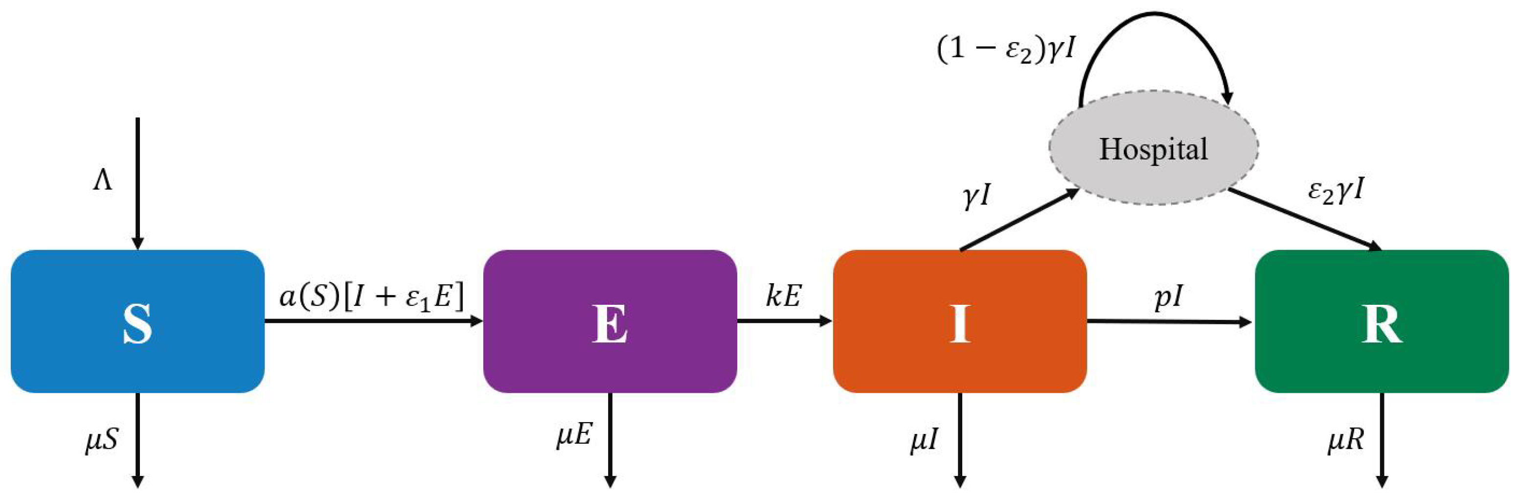
To better understand the relationships among various groups in model (1), we present the flowchart Figure 1 of the corresponding deterministic model for model (1).

It is noted that diseases such as influenza, varicella and dengue fever may exhibit periodic outbreaks due to cyclic changes in vector behavior, seasonal factors, or human lifestyle habits. In view of this, some scholars have considered periodic variations for studying stochastic periodic models [34,35,36,37,38,39]. For instance, Shangguan et al. [38] further considered periodic variations in a stochastic model with infectivity in the incubation period and home isolation, constructed a periodic model, and then identified the existence of T-periodic solutions.

This paper builds upon the research of Zhang et al. [29] to further discuss the conditions that contribute to disease persistence and the existence of stationary distributions in model (1). Since the transmission model (1) is unidirectional and individuals in the R-class do not flow back to any other compartment, removing the R-class to produce model (2) does not affect the dynamics of the remaining variables,

$$\left\{\begin{array}{c}dS\left(t\right)=\left\{\Lambda -\mu S\left(t\right)-a\left(S\left(t\right)\right)\left[I\left(t\right)+{\epsilon }_{1}E\left(t\right)\right]\right\}dt+{\sigma }_{1}S\left(t\right)d{B}_1\left(t\right),\hfill \\ dE\left(t\right)=\left\{a\left(S\left(t\right)\right)\left[I\left(t\right)+{\epsilon }_{1}E\left(t\right)\right]-(\mu +k)E\left(t\right)\right\}dt+{\sigma }_{2}E\left(t\right)d{B}_2\left(t\right),\hfill \\ dI\left(t\right)=[kE\left(t\right)-(\mu +p+\gamma )I\left(t\right)]dt+{\sigma }_{3}I\left(t\right)d{B}_3\left(t\right).\hfill \end{array}\right.$$

(2)

The complete dynamic equations for S, E, and I are retained in model (2), ensuring that the core mechanisms of disease transmission are preserved.

In addition, this paper proposes a stochastic semi-parametric SEIR model (3) with periodic coefficients corresponding to model (2),

$$\left\{\begin{array}{c}dS\left(t\right)=\left\{\Lambda \left(t\right)-\mu \left(t\right)S\left(t\right)-a^{\circ }(S,t)\left[I\left(t\right)+{\epsilon }_{1}E\left(t\right)\right]\right\}dt+{\sigma }_1\left(t\right)S\left(t\right)d{B}_1\left(t\right),\hfill \\ dE\left(t\right)=\left\{a^{\circ }(S,t)\left[I\left(t\right)+{\epsilon }_{1}E\left(t\right)\right]-(\mu \left(t\right)+k\left(t\right))E\left(t\right)\right\}dt+{\sigma }_2\left(t\right)E\left(t\right)d{B}_2\left(t\right),\hfill \\ dI\left(t\right)=[k\left(t\right)E\left(t\right)-(\mu \left(t\right)+p\left(t\right)+\gamma \left(t\right))I\left(t\right)]dt+{\sigma }_3\left(t\right)I\left(t\right)d{B}_3\left(t\right),\hfill \end{array}\right.$$

(3)

we further discuss the conditions for the existence of periodic solutions in model (3). In this model, the instantaneous disease transmission rate is defined as a bivariate periodic function: $a^{\circ }(S,t)={\sum }_{i=1}^m{\kappa }_i\left(t\right)f_i\left(S\right)+c_i$, where $c_i$ are constants, $f_i\left(S\right)$ satisfy piecewise continuity conditions, and ${\kappa }_i\left(t\right),\Lambda \left(t\right),\mu \left(t\right),p\left(t\right),\gamma \left(t\right),k\left(t\right)$ and noise intensities ${\sigma }_j\left(t\right)(j=1,2,3)$ are continuous T-periodic functions.

The hypothesis in reference [29] states that the bounded instantaneous disease transmission rate $a\left(S\right)$ satisfies $a\left(S\left(0\right)\right)=0,\left(S\left(t\right)\right)\ge a^{\prime }\left(S\left(t\right)\right)>0$, which leads to the existence and uniqueness of the overall positive solution of model (1), the sufficient conditions for disease extinction, and the sufficient conditions for solutions to asymptotically approach the disease-free equilibrium point in deterministic models. However, it does not provide sufficient conditions for the persistent existence of the disease. Therefore, this paper modifies the assumption of the instantaneous transmission rate $a\left(S\right(t\left)\right)$ in model (2) to derive sufficient conditions for the persistence and existence of a stationary distribution of the disease. Similarly, for the instantaneous transmission rate $a^{\circ }(S,t)$ of a periodically occurring disease, sufficient conditions for the existence of positive periodic solutions in model (3) can be derived.

For the convenience of the subsequent proof, we make the following assumptions in this paper.

Assumption 1.

The instantaneous disease transmission rate $a\left(S\right)$ that satisfies the local Lipschitz condition also meets the criteria for $a\left(0\right)=0$ and $M_1\le \frac{a\left(s\right)}{s}\le M_2$, where $0<M_1\le M_2$.

Assumption 2.

The instantaneous disease transmission rate $a^{\circ }(S,t)$ that satisfies the local Lipschitz condition also meets the criteria $a^{\circ }(0,t)=0$ and $M_1^{\circ }\le \frac{a^{\circ }(S,t)}{S}\le M_2^{\circ }$, where $0<M_1^{\circ }\le M_2^{\circ }$.

These conditions constrain the ratio of the infection rate to the size of the susceptible population, indicating that the infection rate is approximately linear, with the proportionality coefficient fluctuating within the interval $\left[M_1,M_2\right]$, reflecting the heterogeneity of disease transmission. For example, $M_1$ can represent low transmission efficiency under periods of strict isolation, such as during the COVID-19 lockdowns, while $M_2$ corresponds to high transmission efficiency in the absence of interventions.

The paper is structured as follows. Section 2 establishes the conditions for the persistence of the disease within the stochastic SEIR model (2), accompanied by numerical verification. In Section 3, we conclude that the stochastic SEIR model (2) possesses a unique ergodic stationary distribution, which is further supported by numerical validation. Section 4 investigates the existence of positive periodic solutions for the stochastic periodic model (3), with analytical results confirmed through simulations.

2. Persistence of the Model (2)

Under Assumption 1, similarly to Zhang et al. [29], we can establish the existence and uniqueness of global solutions and the dynamics of extinction for the stochastic SEIR model (2). Building upon this foundation, we extend Zhang et al.’s framework [29] to investigate the persistence of the disease in model (2).

Lemma 1.

For any given initial value $X\left(0\right):=\left(S\right(0),E(0),I(0\left)\right)$$\in R_{+}^3$, model (2) admits a unique solution $X\left(t\right):=\left(S\right(t),E(t),I(t\left)\right)$ for $t\ge 0$, and this solution remains in $R_{+}^3$ with a probability of one.

Proof. 

It is noted that all coefficients of system (2) are locally Lipschitz-continuous. Therefore, for any initial value $(S\left(0\right),E\left(0\right),I\left(0\right))\in R_{+}^3$, there exists a unique local solution $(S\left(t\right),E\left(t\right),I\left(t\right))\in \left[0,{\tau }_e\right)$ [40]. Next, we demonstrate that this solution is global. For any $(S,E,I)\in R_3^{+}$, we define a non-negative $C^2$ function $V(S,E,I):R_{+}^3\to R_{+}$

$$V(S,E,I):=\left(S-o_1-o_1\ln \frac{S}{o_1}\right)+(E-1-\ln E)+o_2(I-1-\ln I),$$

(4)

where the parameters $o_1$ and $o_2$ are given by

$$o_1=\frac{(\mu +p+\gamma )(\mu +k)}{\left[k+{\epsilon }_1(\mu +p+\gamma )\right]M_2},o_2=\frac{\mu +k}{\left[k+{\epsilon }_1(\mu +p+\gamma )\right]M_2}.$$

(5)

The non-negativity of the function is ensured by the condition $x>0$, which guarantees that $x-1-\ln x>0$. The choice of weights $\left(\frac{(\mu +p+\gamma )(\mu +k)}{\left[k+{\epsilon }_1(\mu +p+\gamma )\right]M_2},1,\frac{\mu +k}{\left[k+{\epsilon }_1(\mu +p+\gamma )\right]M_2}\right)$ is related to the system’s equilibrium point and the transmission dynamics. By balancing the drift and diffusion terms, the $LV$ can be controlled at the boundary.

Using Itô’ s formula, the differential $dV(S,E,I)$ can be expanded as

$$dV(S,E,I)=LV(S,E,I)dt+{\sigma }_1(S-o_1)d{B}_1+{\sigma }_2(E-1)d{B}_2+o_2{\sigma }_3(I-1)d{B}_3,$$

(6)

where

$$\begin{array}{cc}\hfill LV(S,E,I)=& \left(1-\frac{o_1}{S}\right)\left[\Lambda -\mu S-a\left(S\right)\left(I+{\epsilon }_{1}E\right)\right]+\frac{o_1}{2}\frac{1}{S^2}{\sigma }_1^2{S}^2+\left(1-\frac{1}{E}\right)\left[a\left(S\right)\left(I+{\epsilon }_{1}E\right)-(\mu +k)E\right]+\frac{1}{2}\frac{1}{E^2}{\sigma }_2^2{E}^2\hfill \\ \hfill & +o_2\left(1-\frac{1}{I}\right)[kE-(\mu +p+\gamma )I]+\frac{o_2}{2}\frac{1}{I^2}{\sigma }_3^2{I}^2\hfill \\ \hfill \le & \Lambda +o_1\mu +2\mu +k+p+\gamma +\frac{o_1{\sigma }_1^2+{\sigma }_2^2+o_2{\sigma }_3^2}{2}+\left[o_{2}k+o_1{\epsilon }_1{M}_2-(\mu +k)\right]E+\left[o_1{M}_2-o_2(\mu +p+\gamma )\right]I,\hfill \end{array}$$

(7)

From the definitions of $o_1$ and $o_2$, it follows that

$$LV(S,E,I)\le \Lambda +o_1\mu +2\mu +k+p+\gamma +\frac{o_1{\sigma }_1^2+{\sigma }_2^2+o_2{\sigma }_3^2}{2}:=K.$$

(8)

The remainder of the proof follows a procedure analogous to Theorem 1 in Zhang et al. [29]. □

Definition 1.

If $\underset{t\to \infty }{\lim }(E\left(t\right)+I\left(t\right))=0$, then model (2) is said to be extinct.

Lemma 2.

For any initial values $X\left(0\right)\in R_{+}^3$, let $X\left(t\right))$ be the solution of model (2). If $R_1:=\frac{2{(k+\mu )}^2\left(1+{\epsilon }_1\right)\Lambda M_2}{\mu \left[k^2\frac{{\sigma }_2^2}{2}\wedge {(k+\mu )}^2\left(\mu +p+\gamma +\frac{{\sigma }_3^2}{2}\right)\right]}<1$, then we can find that

$$\begin{array}{c}\hfill {\displaystyle \underset{t\to +\infty }{\lim }}\sup \frac{\ln [kE+(k+\mu \left)I\right]}{t}\le \frac{k^2\frac{{\sigma }_2^2}{2}\wedge {(k+\mu )}^2\left(\mu +p+\gamma +\frac{{\sigma }_3^2}{2}\right)}{2{(k+\mu )}^2}\left(R_1-1\right)<0.\end{array}$$

(9)

Proof. 

For model (2), we have

$$\begin{array}{cc}\hfill d\left(S\right(t)+E(t)+I(t\left)\right)& =[\Lambda -\mu (S\left(t\right)+E\left(t\right)+I\left(t\right))-(p+\gamma )I\left(t\right)]dt+d{B}_1\left(t\right)+{\sigma }_{2}d{B}_3\left(t\right)+{\sigma }_{3}d{B}_2\left(t\right)\hfill \\ \hfill & \le [\Lambda -\mu (S\left(t\right)+E\left(t\right)+I\left(t\right))]dt+d{B}_1\left(t\right)+{\sigma }_{2}d{B}_3\left(t\right)+{\sigma }_{3}d{B}_2\left(t\right).\hfill \end{array}$$

(10)

then

$$\begin{array}{cc}\hfill \frac{S\left(t\right)+E\left(t\right)+I\left(t\right)}{t}-\frac{S\left(0\right)+E\left(0\right)+I\left(0\right)}{t}\le & \Lambda -\frac{\mu }{t}{\int }_0^t(S\left(s\right)+E\left(s\right)+I\left(s\right))ds+{\sigma }_1\frac{1}{t}{\int }_0^{t}S\left(s\right)d{B}_1\left(s\right)\hfill \\ & +{\sigma }_2\frac{1}{t}{\int }_0^{t}E\left(s\right)d{B}_2\left(s\right)+{\sigma }_3\frac{1}{t}{\int }_0^{t}I\left(s\right)d{B}_3\left(s\right).\hfill \end{array}$$

(11)

From Lemma 2.2 of [18], we have

$$\underset{t\to \infty }{\lim }S\left(t\right)+E\left(t\right)+I\left(t\right)<+\infty ,$$

(12)

$$\underset{t\to \infty }{\lim }\frac{S\left(\mathrm{t}\right)}{t}=\underset{t\to \infty }{\lim }\frac{\mathrm{E}\left(\mathrm{t}\right)}{t}=\underset{t\to \infty }{\lim }\frac{\mathrm{I}\left(\mathrm{t}\right)}{t}=0,$$

(13)

$$\underset{t\to \infty }{\lim }\frac{\ln \mathrm{S}\left(\mathrm{t}\right)}{t}=\underset{t\to \infty }{\lim }\frac{\ln \mathrm{E}\left(\mathrm{t}\right)}{t}=\underset{t\to \infty }{\lim }\frac{\ln \mathrm{I}\left(\mathrm{t}\right)}{t}=0,$$

(14)

$$\underset{t\to \infty }{\lim }\frac{1}{t}{\int }_0^{t}S\left(s\right)d{B}_1\left(s\right)=\underset{t\to \infty }{\lim }\frac{1}{t}{\int }_0^{t}E\left(s\right)d{B}_2\left(s\right)=\underset{t\to \infty }{\lim }\frac{1}{t}{\int }_0^{t}I\left(s\right)d{B}_3\left(s\right)=0,$$

(15)

then

$$\underset{t\to \infty }{\lim \sup }\frac{1}{t}{\int }_0^t(S\left(s\right)+E\left(s\right)+I\left(s\right))ds\le \frac{\Lambda }{\mu }.$$

(16)

Therefore,

$$\underset{t\to \infty }{\lim }\frac{1}{t}{\int }_0^{t}S\left(s\right)ds\le \underset{t\to \infty }{\lim \sup }\frac{1}{t}{\int }_0^t(S\left(s\right)+E\left(s\right)+I\left(s\right))ds\le \frac{\Lambda }{\mu }.$$

(17)

Applying Itô’s formula, we have

$$\begin{array}{cc}\hfill L\left[\ln \right(kE+(\mu +k)I\left)\right]& =\frac{ka\left(S\right)\left(I+{\epsilon }_{1}E\right)}{kE+(\mu +k)I}-\frac{2(\mu +k)(\mu +p+\gamma )I[kE+(\mu +k)I]+k^2{\sigma }_2^2{E}^2+{(k+\mu )}^2{\sigma }_3^2{I}^2}{2{[kE+(\mu +k)I]}^2}\hfill \\ \hfill & \begin{array}{c}\hfill \le a\left(S\right)\left(1+{\epsilon }_1\right)-\frac{k^2\frac{{\sigma }_2^2}{2}\wedge {(k+\mu )}^2\left(\mu +p+\gamma +\frac{{\sigma }_3^2}{2}\right)}{2{(k+\mu )}^2},\end{array}\hfill \end{array}$$

(18)

then

$$\begin{array}{cc}\hfill d\left[\ln \right(kE+(\mu +k)I\left)\right]\le & \left[a\left(S\right)\left(1+{\epsilon }_1\right)-\frac{k^2\frac{{\sigma }_2^2}{2}\wedge {(k+\mu )}^2\left(\mu +p+\gamma +\frac{{\sigma }_3^2}{2}\right)}{2{(k+\mu )}^2}\right]dt\hfill \\ \hfill & +\frac{kE{\sigma }_2}{kE+(\mu +k)I}d{B}_2\left(t\right)+\frac{(\mu +k)I{\sigma }_3}{kE+(\mu +k)I}d{B}_3\left(t\right).\hfill \end{array}$$

(19)

We obtain

$$\begin{array}{cc}\hfill \frac{\ln \left(kE\right(t)+(\mu +k\left)I\right(t\left)\right)-\ln \left(kE\right(0)+(\mu +k\left)I\right(0\left)\right)}{t}\le & \left(1+{\epsilon }_1\right)M_2{\int }_0^{t}S\left(s\right)ds-\frac{k^2\frac{{\sigma }_2^2}{2}\wedge {(k+\mu )}^2\left(\mu +p+\gamma +\frac{{\sigma }_3^2}{2}\right)}{2{(k+\mu )}^2}\hfill \\ & +\frac{1}{t}{\int }_0^t\frac{kE{\sigma }_2}{kE+(\mu +k)I}d{B}_2\left(s\right)+\frac{1}{t}{\int }_0^t\frac{(\mu +k)I{\sigma }_3}{kE+(\mu +k)I}d{B}_3\left(s\right)\hfill \\ \hfill \le & \frac{\left(1+{\epsilon }_1\right)M_2\Lambda }{\mu }-\frac{k^2\frac{{\sigma }_2^2}{2}\wedge {(k+\mu )}^2\left(\mu +p+\gamma +\frac{{\sigma }_3^2}{2}\right)}{2{(k+\mu )}^2}\hfill \\ \hfill =& \frac{k^2\frac{{\sigma }_2^2}{2}\wedge {(k+\mu )}^2\left(\mu +p+\gamma +\frac{{\sigma }_3^2}{2}\right)}{2{(k+\mu )}^2}\left(R_1-1\right)<0.\hfill \end{array}$$

(20)

Therefore, $\underset{t\to \infty }{\lim }[kE\left(t\right)+(\mu +k)I\left(t\right)]=0$. □

Definition 2.

If ${\displaystyle \underset{t\to \infty }{\lim \inf }}\frac{1}{t}{\int }_0^{t}I\left(s\right)ds>0$, then model (2) is said to be persistent in the mean.

Theorem 1.

If $R_2:=\frac{k\Lambda M_1}{\left(\mu +\frac{1}{2}{{\sigma }_1}^2\right)\left(\mu +k+\frac{1}{2}{{\sigma }_2}^2\right)\left(\mu +p+\gamma +\frac{1}{2}{{\sigma }_3}^2\right)}>1$, then the following lower bound is almost certain to hold

$$\underset{t\to +\infty }{\lim }\inf \frac{1}{t}{\int }_0^{t}I\left(s\right)ds\ge \frac{k\left(\mu +k+\frac{1}{2}{\sigma }_2^2\right)\left(R_2-1\right)}{b_{1}k{M}_2+b_1{\epsilon }_1{M}_2(\mu +p+\gamma )}>0.$$

(21)

Proof. 

Integrate both sides of the third equation in model (2) from 0 to t, divide by t, and rearrange to obtain

$$\frac{I\left(t\right)-I\left(0\right)}{t}=\frac{1}{t}{\int }_0^{t}kE\left(s\right)ds-\frac{1}{t}{\int }_0^t(\mu +p+\gamma )I\left(s\right)ds+\frac{{\sigma }_3}{t}{\int }_0^{t}I\left(s\right)d{B}_3\left(s\right).$$

(22)

Rearranging terms yields

$$\begin{array}{cc}\hfill \frac{1}{t}{\int }_0^{t}E\left(s\right)ds& =\frac{\mu +p+\gamma }{kt}{\int }_0^{t}I\left(s\right)ds+\frac{I\left(t\right)-I\left(0\right)}{kt}-\frac{{\sigma }_3}{kt}{\int }_0^{t}I\left(s\right)d{B}_3\left(s\right)\hfill \\ \hfill & =\frac{\mu +p+\gamma }{kt}{\int }_0^{t}I\left(s\right)ds+\phi \left(t\right),\hfill \end{array}$$

(23)

where

$$\phi \left(t\right):=\frac{I\left(t\right)-I\left(0\right)}{kt}-\frac{{\sigma }_3}{kt}{\int }_0^{t}I\left(s\right)d{B}_3\left(s\right),$$

(24)

and it follows that $\underset{t\to +\infty }{\lim }\frac{\phi \left(t\right)}{t}=0$; this is almost certain.

Define the auxiliary function $F(S,E,I):R_{+}^3\to R$

$$F(S,E,I):=-b_1\ln S-b_2\ln I-\ln E,$$

(25)

where the coefficients $b_1$ and $b_2$ are given by

$$b_1:=\frac{k\Lambda M_1}{{\left(\mu +\frac{1}{2}{{\sigma }_1}^2\right)}^2\left(\mu +p+\gamma +\frac{1}{2}{{\sigma }_3}^2\right)},b_2:=\frac{k\Lambda M_1}{\left(\mu +\frac{1}{2}{{\sigma }_1}^2\right){\left(\mu +p+\gamma +\frac{1}{2}{{\sigma }_3}^2\right)}^2}.$$

(26)

Applying Itô’s formula to $F(S,E,I)$, we derive

$$dF=LFdt-b_1{\sigma }_{1}d{B}_1\left(t\right)-b_2{\sigma }_{3}d{B}_3\left(t\right)-{\sigma }_{2}d{B}_2\left(t\right),$$

(27)

where

$$\begin{array}{cc}\hfill LF& =b_1\frac{a\left(S\right)}{S}\left(I+{\epsilon }_{1}E\right)-b_1\frac{\Lambda }{S}-b_{2}k\frac{E}{I}-a\left(S\right)\frac{I}{E}-{\epsilon }_{1}a\left(S\right)E+b_1\mu \hfill \\ \hfill & +b_2(\mu +p+\gamma )+(\mu +k)+\frac{1}{2}{b}_1{\sigma }_1^2+\frac{1}{2}{b}_2{\sigma }_3^2+\frac{1}{2}{\sigma }_2^2\hfill \\ \hfill & \le b_1{M}_{2}I+b_1{\epsilon }_1{M}_{2}E-3\sqrt[3]{b_1{b}_{2}k\Lambda M_1}+b_1\left(\mu +\frac{1}{2}{\sigma }_1^2\right)+b_2\left(\mu +p+\gamma +\frac{1}{2}{\sigma }_3^2\right)\hfill \\ \hfill & +\left(\mu +k+\frac{1}{2}{\sigma }_2^2\right)=b_1{M}_{2}I+b_1{\epsilon }_1{M}_{2}E-\left(\mu +k+\frac{1}{2}{\sigma }_2^2\right)\left(R_2-1\right).\hfill \end{array}$$

(28)

Consequently,

$$dF\le \left[b_1{M}_{2}I+b_1{\epsilon }_1{M}_{2}E-\left(\mu +k+\frac{1}{2}{\sigma }_2^2\right)\left(R_2-1\right)\right]dt-b_1{\sigma }_{1}d{B}_1\left(t\right)-b_2{\sigma }_{3}d{B}_3\left(t\right)-{\sigma }_{2}d{B}_2\left(t\right).$$

(29)

Integrate both sides of the inequality from 0 to t and divide by t,

$$\begin{array}{cc}\hfill \frac{F\left(t\right)-F\left(0\right)}{t}& \le \left[b_1{M}_2\frac{1}{t}{\int }_0^{t}I\left(s\right)ds+b_1{\epsilon }_1{M}_2\frac{1}{t}{\int }_0^{t}E\left(s\right)ds\right]-\left(\mu +k+\frac{1}{2}{\sigma }_2^2\right)\left(R_2-1\right)\hfill \\ \hfill & -\frac{1}{t}\left[b_1{\sigma }_1{\int }_0^{t}d{B}_1\left(s\right)\begin{array}{c}\hfill +b_2{\sigma }_3{\int }_0^{t}d{B}_3\left(s\right)+{\sigma }_2{\int }_0^{t}d{B}_2\left(s\right)\end{array}\right].\hfill \end{array}$$

(30)

From the relation

$$\frac{1}{t}{\int }_0^{t}E\left(s\right)ds=\frac{\mu +p+\gamma }{kt}{\int }_0^{t}I\left(s\right)ds+\phi \left(t\right),$$

(31)

we derive

$$\begin{array}{cc}\hfill \frac{F\left(t\right)-F\left(0\right)}{t}& \le \frac{b_{1}k{M}_2+b_1{\epsilon }_1{M}_2(\mu +p+\gamma )}{k}\frac{1}{t}{\int }_0^{t}I\left(s\right)ds-\left(\mu +k+\frac{1}{2}{\sigma }_2^2\right)\left(R_2-1\right)\hfill \\ \hfill & +b_1{\epsilon }_1{M}_2\phi \left(t\right)-\frac{1}{t}\left[b_1{\sigma }_1{\int }_0^{t}d{B}_1\left(s\right)\begin{array}{c}\hfill +b_2{\sigma }_3{\int }_0^{t}d{B}_3\left(s\right)+{\sigma }_2{\int }_0^{t}d{B}_2\left(s\right)\end{array}\right].\hfill \end{array}$$

(32)

Since $\underset{t\to +\infty }{\lim }\frac{\phi \left(t\right)}{t}=0$ almost certainly and the noise terms satisfy $\underset{t\to +\infty }{\lim }\frac{1}{t}{\int }_0^{t}d{B}_i\left(s\right)=0$, rearranging terms yields

$$\underset{t\to +\infty }{\lim }\inf \frac{1}{t}{\int }_0^{t}I\left(s\right)ds\ge \frac{k\left(\mu +k+\frac{1}{2}{\sigma }_2^2\right)\left(R_2-1\right)}{b_{1}k{M}_2+b_1{\epsilon }_1{M}_2(\mu +p+\gamma )}.$$

(33)

This establishes the non-negativity of the time-averaged infected population. □

Numerical Simulations. To support the validity and efficiency of the analytical results provided in the preceding section, we will construct a numerical technique to simulate the solution path of model (2). We demonstrate the correctness of the obtained results by enumerating specific transfer functions and performing numerical simulations using the Milstein higher-order method, thereby illustrating the impact of different specific factors in the model on the disease. Assuming $N^{\ast }\in \mathbb{N},m=$$1,2,3,n=1,2,\dots ,N^{\ast },\Delta t=\frac{T}{N^{\ast }}$ represents the size of the time step in the interval $[0,T]$. Additionally, $\Delta B_n\triangleq B\left(t_{n+1}\right)-$$B\left(t_n\right)=\sqrt{\Delta t}{\xi }_{mn}$, where ${\xi }_{mn}$ is considered an independent Gaussian random variable $N(0,1)$. Therefore, the Milstein method associated with model (2) takes the following form,

$$\begin{array}{c}\hfill \left\{\begin{array}{c}S(n+1)=S\left(n\right)+\left\{\Lambda -\mu S\left(n\right)-a\left(S\left(n\right)\right)\left[I\left(n\right)+{\epsilon }_{1}E\left(n\right)\right]\right\}\Delta t+{\sigma }_{1}S\left(n\right){\xi }_{1n}\sqrt{\Delta t}+\frac{{\sigma }_1^2}{2}S\left(n\right)\left(\Delta {\xi }_{1n}^2-1\right)\Delta t,\hfill \\ E(n+1)=E\left(n\right)+\left\{a\left(S\left(n\right)\right)\left[I\left(n\right)+{\epsilon }_{1}E\left(n\right)\right]-(\mu +k)E\left(n\right)\right\}\Delta t+{\sigma }_{1}E\left(n\right){\xi }_{2n}\sqrt{\Delta t}+\frac{{\sigma }_2^2}{2}E\left(n\right)\left(\Delta {\xi }_{2n}^2-\Delta t\right),\hfill \\ I(n+1)=I\left(n\right)+[kE\left(n\right)-(\mu +p+\gamma )I\left(n\right)]\Delta t+{\sigma }_{1}I\left(n\right){\xi }_{3n}\sqrt{\Delta t}+\frac{{\sigma }_2^2}{2}I\left(n\right)\left(\Delta {\xi }_{3n}^2-\Delta t\right).\hfill \end{array}\right.\end{array}$$

(34)

The initial population $X\left(0\right)=(S\left(0\right),E\left(0\right),I\left(0\right))\in R_{+}^3$ primarily influences the short-term dynamics of the simulation, such as the speed of outbreak and peak, but does not significantly affect the long-term simulation outcomes, as the model’s global stability, parameter dominance, and randomness smooth out initial differences. Therefore, we consider a population with an initial count of 995,000 susceptibles, 3000 exposed, and 2000 infected individuals; that is, $\left(\mathrm{S}\right(0)$, $\mathrm{E}\left(0\right),\mathrm{I}\left(0\right))=(0.995,0.003,0.002)$, with $\Delta \mathrm{t}=0.01$. The simulation is conducted using the basic data from the COVID-19 pandemic [19], with the parameter values shown in

Table 2. Estimated parameter values and their epidemiological interpretations for the COVID-19 transmission model.

Param.	Value	Unit	Interpretation	Ref.
$\Lambda$	0.05812	day−1	Recruitment rate (birth/immigration)	[19]
$\mu$	0.00003	day−1	Mortality/emigration rate	[19]
k	0.2	day−1	Latent period ($1/k$ = 5 days)	[19]
p	0.1	day−1	Recovery rate ($1/p$ = 10 days)	[19]
$\gamma$	0.1	day−1	Hospitalization rate	Asm.
${\epsilon }_1$	0.5	–	Exposed individuals’ relative infectivity (50% of infectious)	Asm.

Asm.: assumed values based on the epidemiological characteristics of COVID-19.

.

In order to obtain the critical value of the disease transmission rate that has an average strong persistence in numerical terms, we choose $\left({\sigma }_1,{\sigma }_2,{\sigma }_3\right)=(0.3,0.3,0.3)$ and perform direct substitution to calculate $R_2>1$; thus, we have

$$M_1>\frac{\left(\mu +\frac{1}{2}{\sigma }_1^2\right)\left(\mu +k+\frac{1}{2}{\sigma }_2^2\right)\left(\mu +p+\gamma +\frac{1}{2}{\sigma }_3^2\right)}{k\Lambda }\approx 0.3655.$$

(35)

To validate this viewpoint, this paper first demonstrates the impact of different contact rate functions $a\left(S\right)$ on disease dynamics through four examples with $M_1=0.4$, and then presents the temporal dynamics of the SEI state variables along with the relationship between $a\left(S\right)$ and S in conjunction with the figures. These examples encompass linear, piecewise linear, convex, and concave smooth contact rate functions, indicating that the threshold $R_2\approx 1.10>1$ suggests a strong persistence of the disease on average in all cases. Furthermore, another example that satisfies $R_2\le 1$ but shows disease persistence illustrates that the threshold $R_2>1$ is merely a sufficient condition for the disease to exhibit strong persistence on average.

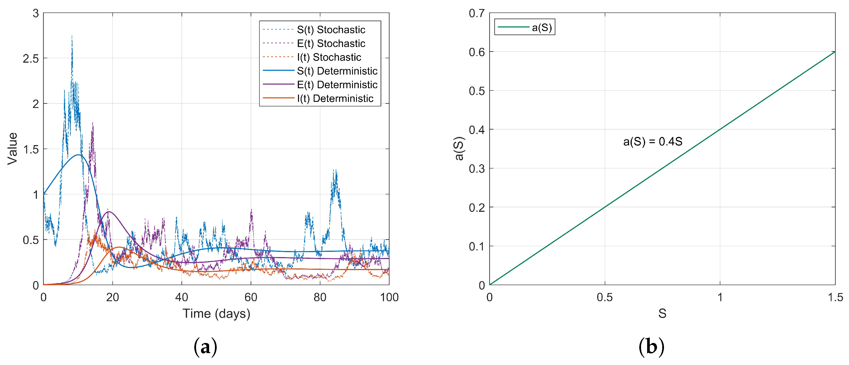
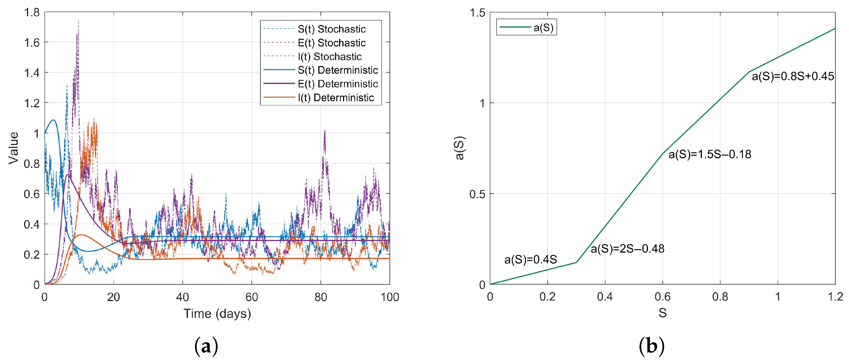
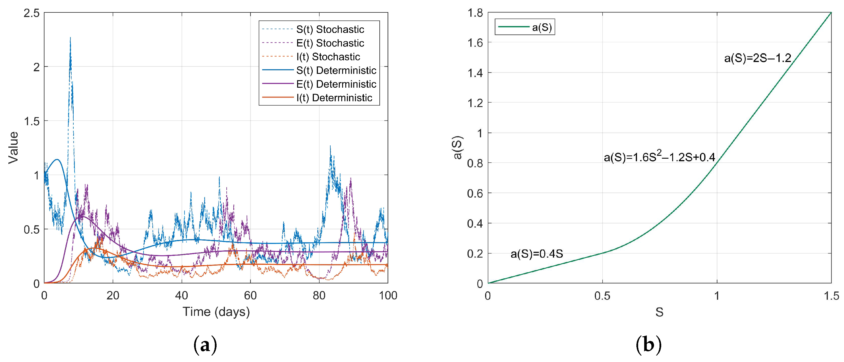
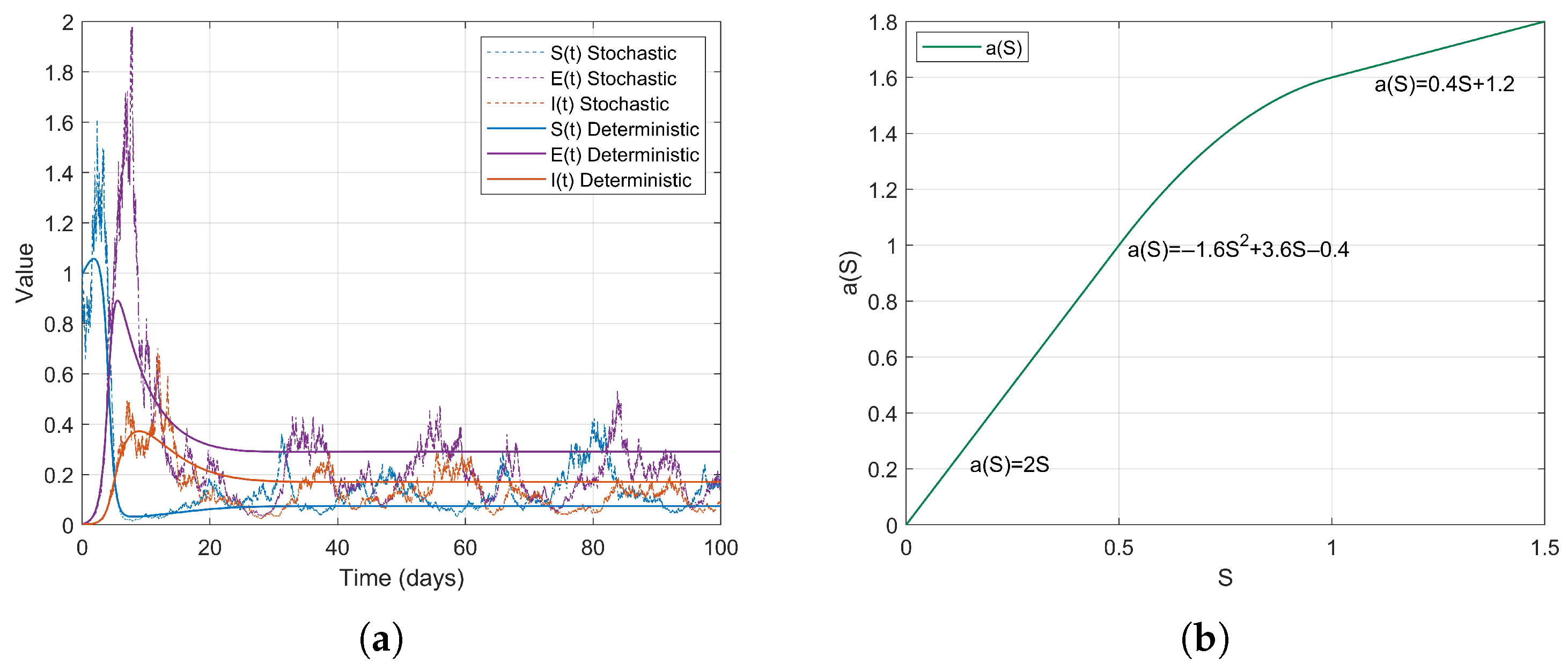
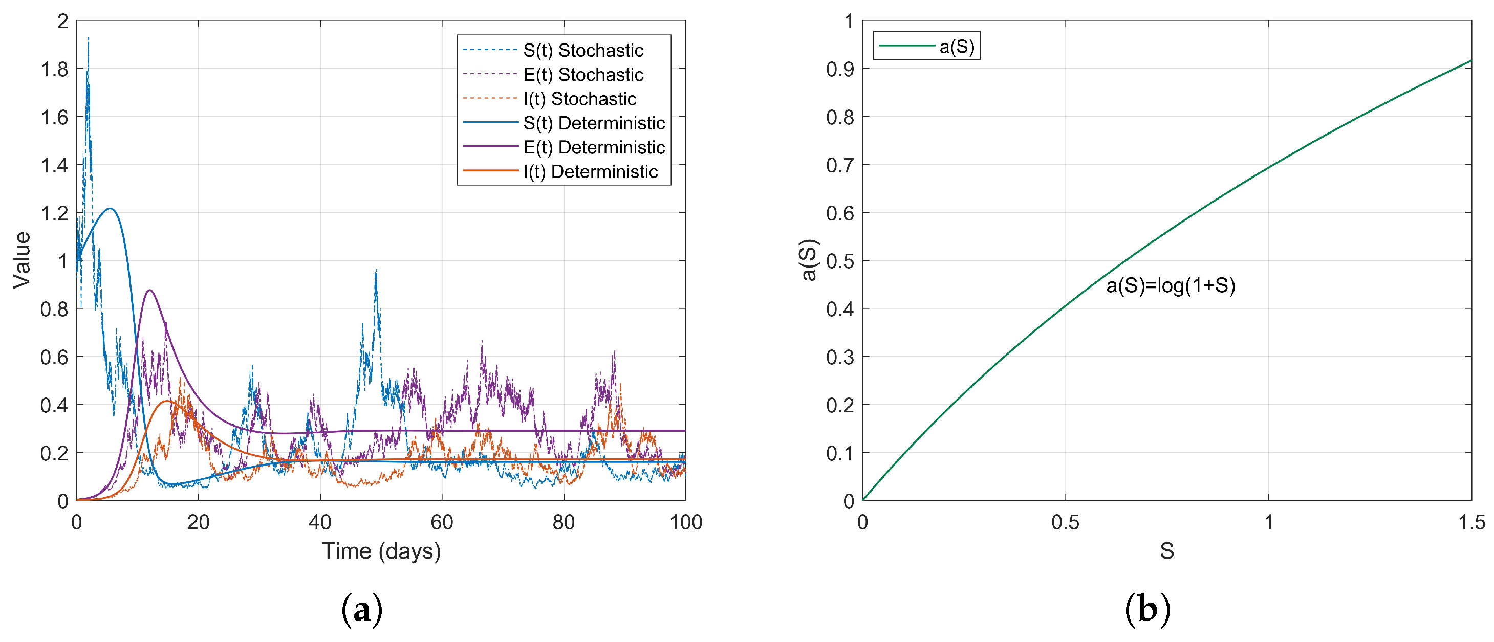
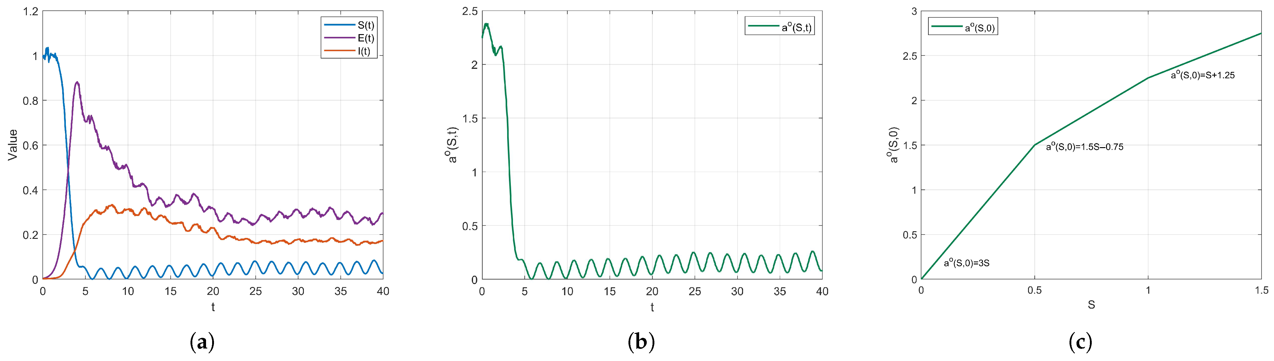
Example 1.

During the early stages of the COVID-19 pandemic, urban areas, particularly dense communities that did not implement social distancing measures, exhibited characteristics of high population density and consistent social mixing rates. It can be assumed that the contact rate increases proportionally with the number of susceptible individuals S. Therefore, we consider a linear contact rate function

$$a\left(S\right)=0.4S,$$

(36)

then $M_1=M_2=0.4$. The simulation results are as follows (Figure 2).

Example 2.

Based on the changes in contact rates corresponding to population thresholds, we can simulate the graded social distancing policies in different regions. For instance, when S is low, contact is minimal; at moderate levels, it increases; and at higher levels, it grows in a controlled manner. Therefore, we define the contact rate as a piecewise linear function

$$a\left(S\right)=\left\{\begin{array}{cc}0.4S,\hfill & \mathit{if}0\le S<0.3,\hfill \\ 2S-0.48,\hfill & \mathit{if}0.3\le S<0.6,\hfill \\ 1.5S-0.18,\hfill & \mathit{if}0.6\le S<0.9,\hfill \\ 0.8S+0.45,\hfill & \mathit{if}S\ge 0.9,\hfill \end{array}\right.$$

(37)

then $M_1=0.4,M_2=2$. The simulation results are as follows (Figure 3).

Example 3.

After the lifting of restrictions, the occurrence of social gatherings intensified, and the contact rate accelerated with the increase in S. For instance, in 2022, as some regions returned to normal life, the contact rate rapidly increased with S. We can simulate this using a convex function. Therefore, we define the contact rate as a piecewise smooth convex function

$$a\left(S\right)=\left\{\begin{array}{cc}0.4S,\hfill & \mathit{if}0\le S<0.5,\hfill \\ 1.6S^2-1.2S+0.4,\hfill & \mathit{if}0.5\le S<1,\hfill \\ 2S-1.2,\hfill & \mathit{if}S\ge 1,\hfill \end{array}\right.$$

(38)

where $a\left(S\right)$ is a convex and increasing function, then $M_1=0.4,M_2=2$. The simulation results are as follows (Figure 4).

Example 4.

In scenarios where social networks are saturated or subject to forced capacity limits, such as during the COVID-19 pandemic at high levels of social interaction $\left(S\right)$, or in situations where crowd control measures are implemented in places like shopping malls, the growth of the contact rate tends to stabilize. Therefore, we define the contact rate as a piecewise smooth concave function

$$\begin{array}{c}\hfill a\left(S\right)=\left\{\begin{array}{cc}2S,\hfill & \mathit{if}0\le S<0.5,\hfill \\ -1.6S^2+3.6S-0.4,\hfill & \mathit{if}0.5\le S<1,\hfill \\ 0.4S+1.2,\hfill & \mathit{if}S\ge 1,\hfill \end{array}\right.\end{array}$$

(39)

where $a\left(S\right)$ is a concave and monotonically increasing function, then $M_1=0.4,M_2=2$. The simulation results are as follows (Figure 5).

Example 5.

For individuals in naturally socially saturated environments or those whose interactions are reduced due to remote work, the contact rate may exhibit a slow increase with respect to S. For instance, in certain regions where face-to-face interactions decreased due to remote work in late 2020, the contact rate gradually increased with S. In this context, a logarithmic function can be considered for modeling, specifically

$$\begin{array}{c}\hfill a\left(S\right)=\ln (1+S).\end{array}$$

(40)

The simulation results are as follows (Figure 6).

The choice of logarithmic functions results in the absence of $M_1>0$, satisfying $M_1\le \frac{\ln (1+S)}{S}\le M_2$. However, as S approaches infinity, $M_1$ approaches 0; thus, R₂ approaches 0. Nevertheless, it is evident from the simulation effect diagrams that strong persistence still exists. This further illustrates that $R_2>1$ is merely a sufficient condition for the disease to exhibit strong persistence on average.

In summary, the different $a\left(S\right)$ functions simulate a range of scenarios, from simple linear propagation to complex nonlinear propagation, encompassing factors such as urbanization, policy interventions, and behavioral changes. The unified result of $R_2>1$ indicates that these functions support strong persistence under various conditions; however, the propagation patterns reveal differences in the timing and intensity of interventions. $M_1$ and $M_2$ are based on the range of $a\left(S\right)$ and reflect the variability of contact rates in reality. This setting can effectively guide real-world epidemic control strategies, such as assessing the effectiveness of isolation or optimizing resource allocation. In particular, $M_1$ is a core parameter for epidemic management, predicting long-term trends and optimizing non-pharmaceutical interventions. Reducing $M_1$ is directly related to the sustainable management of the epidemic.

3. Endemic Stationary Distribution of Model (2)

In the context of stochastic epidemic modeling, analyzing the ergodic stationary distribution is essential for understanding the long-term statistical behavior of a system subjected to random perturbations. Therefore, the objective of this section is to investigate the ergodic stationary distribution of model (2).

Lemma 3.

[41] Let $U\subset E_l$ be a bounded domain with a regular boundary Γ, satisfying the following properties:

(A.1) In U and some neighborhoods of U, the smallest eigenvalue of the diffusion matrix $B\left(x\right)$ is non-vanishing.

(A.2) For $x\in E_l\setminus U$, the mean time τ taken for the trajectory starting at x to reach the set U is finite, and for every compact set $K\subset E_l,\underset{x\in K}{\sup }{E}_x\tau <\infty$.

Then the Markov process $X\left(t\right)$ admits a stationary (invariant) distribution $\mu (·)$. Let $f(·)$ be a function integrable with respect to μ. Then for all $x\in E_l$,

$$P_x\left\{\underset{T\to \infty }{\lim }\frac{1}{T}{\int }_0^{T}f\left(X\left(t\right)\right)dt={\int }_{E_l}f\left(x\right)\mu \left(dx\right)\right\}=1.$$

(41)

Theorem 2.

If $R_2>1$, then for any initial value $X\left(0\right)\in R_{+}^3$, model (2) admits a unique ergodic stationary distribution.

Proof. 

To complete the proof, it is sufficient to verify conditions (A.1) and (A.2) in the Lemma 3. The diffusion matrix of model (2) is $B=\left(\begin{array}{ccc}{{\sigma }_1}^2{S}^2& 0& 0\\ 0& {{\sigma }_2}^2{E}^2& 0\\ 0& 0& {{\sigma }_3}^2{I}^2\end{array}\right)$. There exists a constant $M={\displaystyle \underset{(S,E,I)\in \overline{U}\subset R_{+}^3}{\min }}\left\{{{\sigma }_1}^2{S}^2,{{\sigma }_2}^2{E}^2,{{\sigma }_3}^2{I}^2\right\}>0$, such that for all $(S,E,I)\in \overline{U}$ and any vector $\xi =\left({\xi }_1,{\xi }_2,{\xi }_3\right)\in R^3$, the quadratic form satisfies: ${\sum }_{i,j=1}^3{a}_{ij}(S,E,I){\xi }_i{\xi }_j={{\sigma }_1}^2{S}^2{\xi }_1^2+{{\sigma }_2}^2{E}^2{\xi }_2^2+{{\sigma }_3}^2{I}^2{\xi }_3^2\ge M{\left|\xi \right|}^2$. This inequality confirms that condition (A.1) holds within the domain U. Construct a non-negative $C^2$-function G

$$G\left(X\left(t\right)\right):=M\left(-\ln S-C_1\ln E-C_2\ln I-C_{3}I\right)-\ln S-\ln E+\frac{1}{q+1}{(S+E+I)}^{q+1},$$

(42)

where

$$\begin{array}{c}{C}_1:=\frac{k\Lambda M_1}{{\left(\mu +k+\frac{1}{2}{{\sigma }_2}^2\right)}^2\left(\mu +p+\gamma +\frac{1}{2}{{\sigma }_3}^2\right)},C_2:=\frac{k\Lambda M_1}{\left(\mu +k+\frac{1}{2}{{\sigma }_2}^2\right){\left(\mu +p+\gamma +\frac{1}{2}{{\sigma }_3}^2\right)}^2},\\ C_3:=\frac{{\epsilon }_1}{k}{M}_2,0<q<1,m:=\left[\mu -\frac{q}{2}\left({{\sigma }_1}^2\mathrm{V}{{\sigma }_2}^2\mathrm{V}{{\sigma }_3}^2\right)\right]>0.\end{array}$$

(43)

It is noted that $G\left(X\right(t\left)\right)$ is continuous, and as any of S, E, or I approaches $0^{+}$ or $+\infty$, $G\left(X\right(t\left)\right)$ tends to $+\infty$. This indicates that when ($S,E,I$) approaches the boundary of $R_3^{+},\mathrm{G}\left(\mathrm{X}\left(\mathrm{t}\right)\right)$ tends to $+\infty$. Therefore, $G\left(X\right(t\left)\right)$ must have a lower bound, and it reaches this lower bound at the point $X_0=\left(S_0,E_0,I_0\right)$ within the interior of $R_3^{+}$.

Define $\tilde{G}\left(X\left(t\right)\right)$ as follows

$$\tilde{G}\left(X\left(t\right)\right):=G\left(X\left(t\right)\right)-G\left(X\left(0\right)\right)=M\left(G_1+G_2\right)+G_3+G_4,$$

(44)

where

$$\begin{array}{c}{G}_1:=-\ln S-C_1\ln E-C_2\ln I,G_2:=-C_{3}I,\\ G_3:=\frac{1}{q+1}{(S+E+I)}^{q+1},G_4:=-\ln S-\ln E-G\left(X\left(0\right)\right).\end{array}$$

(45)

From $M_1\le \frac{a\left(s\right)}{s}\le M_2$, we get

$$\begin{array}{cc}\hfill L{G}_1=& -\frac{\Lambda }{S}-C_1\frac{a\left(S\right)}{E}\left(I+{\epsilon }_{1}E\right)-C_{2}k\frac{E}{I}+\frac{a\left(S\right)}{S}\left(I+{\epsilon }_{1}E\right)+\left(\mu +\frac{1}{2}{\sigma }_1^2\right)\hfill \\ \hfill & +C_1\left(\mu +k+\frac{1}{2}{\sigma }_2^2\right)+C_2\left(\mu +p+\gamma +\frac{1}{2}{\sigma }_3^2\right)\hfill \\ \hfill \le & -3\sqrt[3]{C_1{C}_2{M}_{1}k\Lambda }+\frac{a\left(S\right)}{S}I+\frac{a\left(S\right)}{S}{\epsilon }_{1}E+\left(\mu +\frac{1}{2}{\sigma }_1^2\right)\hfill \\ \hfill & +C_1\left(\mu +k+\frac{1}{2}{\sigma }_2^2\right)+C_2\left(\mu +p+\gamma +\frac{1}{2}{\sigma }_3^2\right)\hfill \\ \hfill \le & -\left(\mu +\frac{1}{2}{\sigma }_1^2\right)\left(R_2-1\right)+\frac{a\left(S\right)}{S}I+\frac{a\left(S\right)}{S}{\epsilon }_{1}E\hfill \\ \hfill \le & -\eta +M_{2}I+{\epsilon }_1{M}_{2}E,\hfill \end{array}$$

(46)

$$L{G}_2=-C_3[kE-(\mu +p+\gamma )I]\le -{\epsilon }_1{M}_{2}E+\frac{{\epsilon }_1}{k}(\mu +p+\gamma )M_{2}I,$$

(47)

$$L{G}_3\le \Lambda {(S+E+I)}^q-m{(S+E+I)}^{q+1}\le F_1-\frac{m}{2}{(S+E+I)}^{q+1},$$

(48)

$$L{G}_4\le -\frac{\Lambda }{S}+M_2\left(I+{\epsilon }_{1}E\right)-M_1\frac{S}{E}\left(I+{\epsilon }_{1}E\right)+(2\mu +k)+\frac{1}{2}{\sigma }_1^2+\frac{1}{2}{\sigma }_2^2,$$

(49)

where

$$\eta :=\left(\mu +\frac{1}{2}{\sigma }_1^2\right)\left(R_2-1\right),F_1:=\underset{(S,E,I)\in R_{+}^3}{\sup }\left\{\Lambda {(S+E+I)}^q-\frac{m}{2}{(S+E+I)}^{q+1}\right\}.$$

(50)

Then

$$\begin{array}{cc}\hfill L\tilde{G}\le & \left[-\frac{m}{2}{S}^{q+1}-\frac{\Lambda }{S}+F_1+2\mu +k+\frac{1}{2}{\sigma }_1^2+\frac{1}{2}{\sigma }_2^2\right]+\left[-\frac{m}{2}{E}^{q+1}+{\epsilon }_1{M}_{2}E\right]\hfill \\ \hfill & +\left\{-\frac{m}{2}{I}^{q+1}+M\left\{-\eta +M_2\left[1+\frac{{\epsilon }_1}{k}(\mu +p+\gamma )\right]I\right\}+M_{2}I\right\}-M_1\frac{SI}{E}\hfill \\ \hfill =& g_1\left(S\right)+g_2\left(E\right)+g_3\left(I\right)-M_1\frac{SI}{E},\hfill \end{array}$$

(51)

where

$$g_1\left(S\right):=-\frac{m}{2}{S}^{q+1}-\frac{\Lambda }{S}+F_1+2\mu +k+\frac{1}{2}{\sigma }_1^2+\frac{1}{2}{\sigma }_2^2,$$

(52)

$$g_2\left(E\right):=-\frac{m}{2}{E}^{q+1}+{\epsilon }_1{M}_{2}E,$$

(53)

$$g_3\left(I\right):=-\frac{m}{2}{I}^{q+1}+M\left\{-\eta +M_2\left[1+\frac{{\epsilon }_1}{k}(\mu +p+\gamma )\right]I\right\}+M_{2}I.$$

(54)

Define the bounded closed set

$$D:=\left\{(S,E,I)\in R_{+}^3\left|\epsilon \le S\le \frac{1}{\epsilon }\right.,{\epsilon }^3\le E\le \frac{1}{{\epsilon }^3},\epsilon \le I\le \frac{1}{\epsilon }\right\},$$

(55)

define the functions

$$F_2:=F_1+2\mu +k+\frac{1}{2}{\sigma }_1^2+\frac{1}{2}{\sigma }_2^2,$$

(56)

$$F_3:=\underset{I\in (0,+\infty )}{\sup }\left\{-\frac{m}{4}{I}^{q+1}+M\left\{-\eta +M_2\left[1+\frac{{\epsilon }_1}{k}(\mu +p+\gamma )\right]I\right\}+M_{2}I\right\},$$

(57)

$$F_4:=\underset{E\in (0,+\infty )}{\sup }\left\{-\frac{m}{4}{E}^{q+1}+{\epsilon }_1{M}_{2}E\right\},$$

(58)

where $0<\epsilon <1$ is a sufficiently small constant (not necessarily an integer) satisfying the following conditions:

$$\begin{array}{c}(S,E,I)\in D_1:=\left\{(S,E,I)\in R_{+}^3,0<S<\epsilon \right\},g_2^u+g_3^u+F_2-\frac{\Lambda }{\epsilon }\le -1;\\ (S,E,I)\in D_2:=\left\{(S,E,I)\in R_{+}^3,S>\frac{1}{\epsilon }\right\},g_2^u+g_3^u+F_2-\frac{m}{2{\epsilon }^{q+1}}\le -1;\\ (S,E,I)\in D_3:=\left\{(S,E,I)\in R_{+}^3,I>\frac{1}{\epsilon }\right\},g_1^u+g_2^u+F_3-\frac{m}{4{\epsilon }^{q+1}}\le -1;\\ (S,E,I)\in D_4:=\left\{(S,E,I)\in R_{+}^3,E>\frac{1}{{\epsilon }^3}\right\},g_1^u+g_3^u+F_4-\frac{m}{2{\epsilon }^{3(q+1)}}\le -1;\\ (S,E,I)\in D_5:=\left\{(S,E,I)\in R_{+}^3,0<I<\epsilon \right\},g_1^u+g_2^u+M\left\{-\eta +M_2\left[1+\frac{{\epsilon }_1}{k}(\mu +p+\gamma )\right]\epsilon \right\}+M_2\epsilon \le -1;\\ (S,E,I)\in D_6:=\left\{(S,E,I)\in R_{+}^3,S>\epsilon ,I>\epsilon ,E<{\epsilon }^3\right\},g_1^u+g_2^u+g_3^u-\frac{M_1}{\epsilon }\le -1.\end{array}$$

(59)

Clearly, $R_{+}^3$$\setminus D=D_1\cup D_2\cup D_3\cup D_4\cup D_5\cup D_6$. Synthesizing the above six cases, we will prove that

$$\underset{(S,E,I)\in R_{+}^3\setminus D}{\sup }L\tilde{G}(S,E,I)\le -1.$$

(60)

This completes the proof of (A.2). Consequently, model (2) admits a unique stationary distribution that is ergodic. □

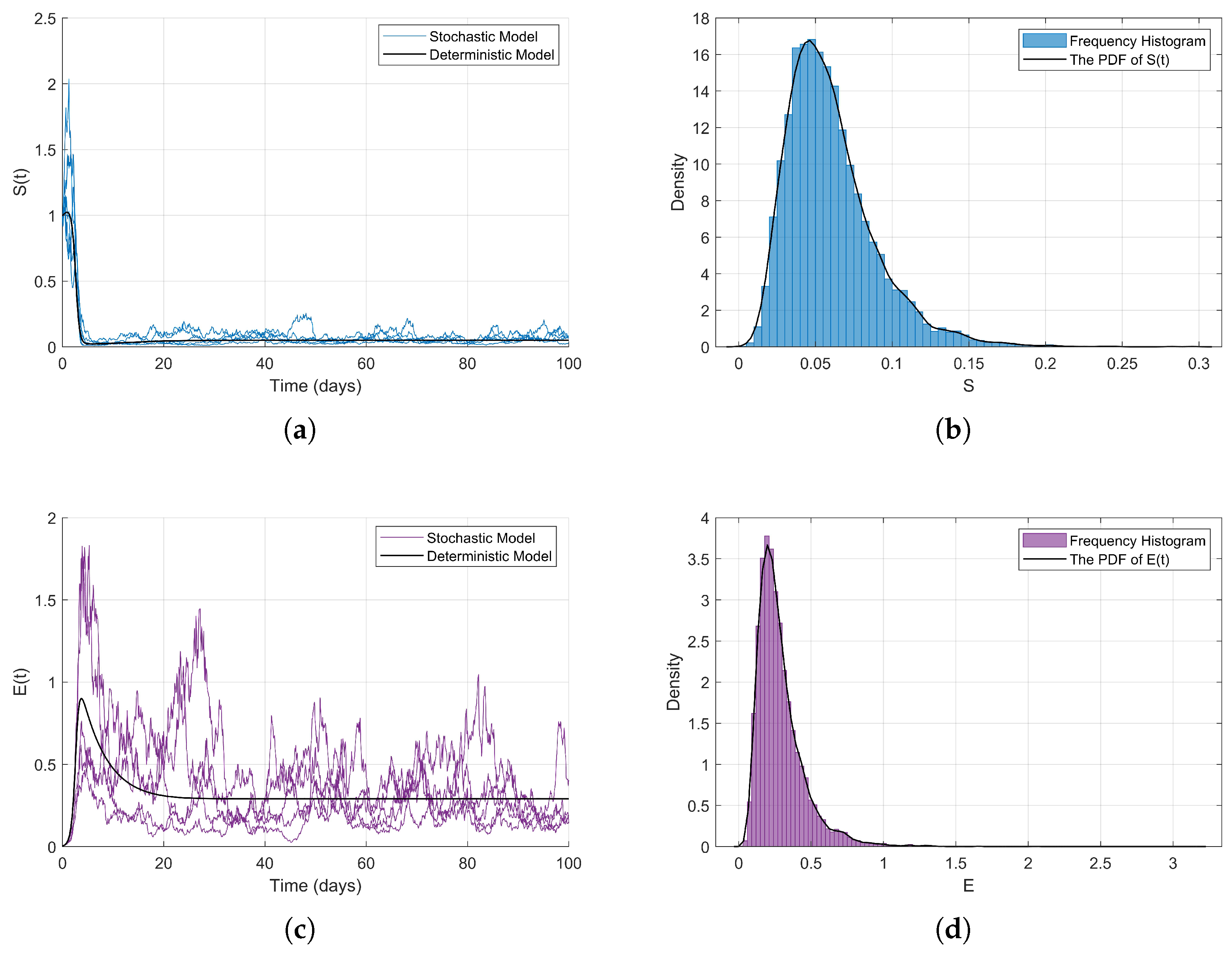
Numerical Simulations. In this part, we adopt the same initial values and parameter configurations as those used in Example 3 to validate the analytical results of Theorem 2 through numerical simulations. We define the contact rate as a piecewise smooth function

$$a\left(S\right)=\left\{\begin{array}{cc}3S,\hfill & \mathit{if}0\le S<1,\hfill \\ -2S^2+5S-0.5,\hfill & \mathit{if}0.5\le S<1,\hfill \\ S+1.5,\hfill & \mathit{if}S\ge 1,\hfill \end{array}\right.$$

(61)

where $a\left(S\right)$ is a concave and increasing function, then $M_1=1,M_2=3$; therefore $R_2\approx 4.30>1$. Therefore, the conditions of Theorem 2 are satisfied, and as illustrated in Figure 7, model (2) exhibits an ergodic stationary distribution.

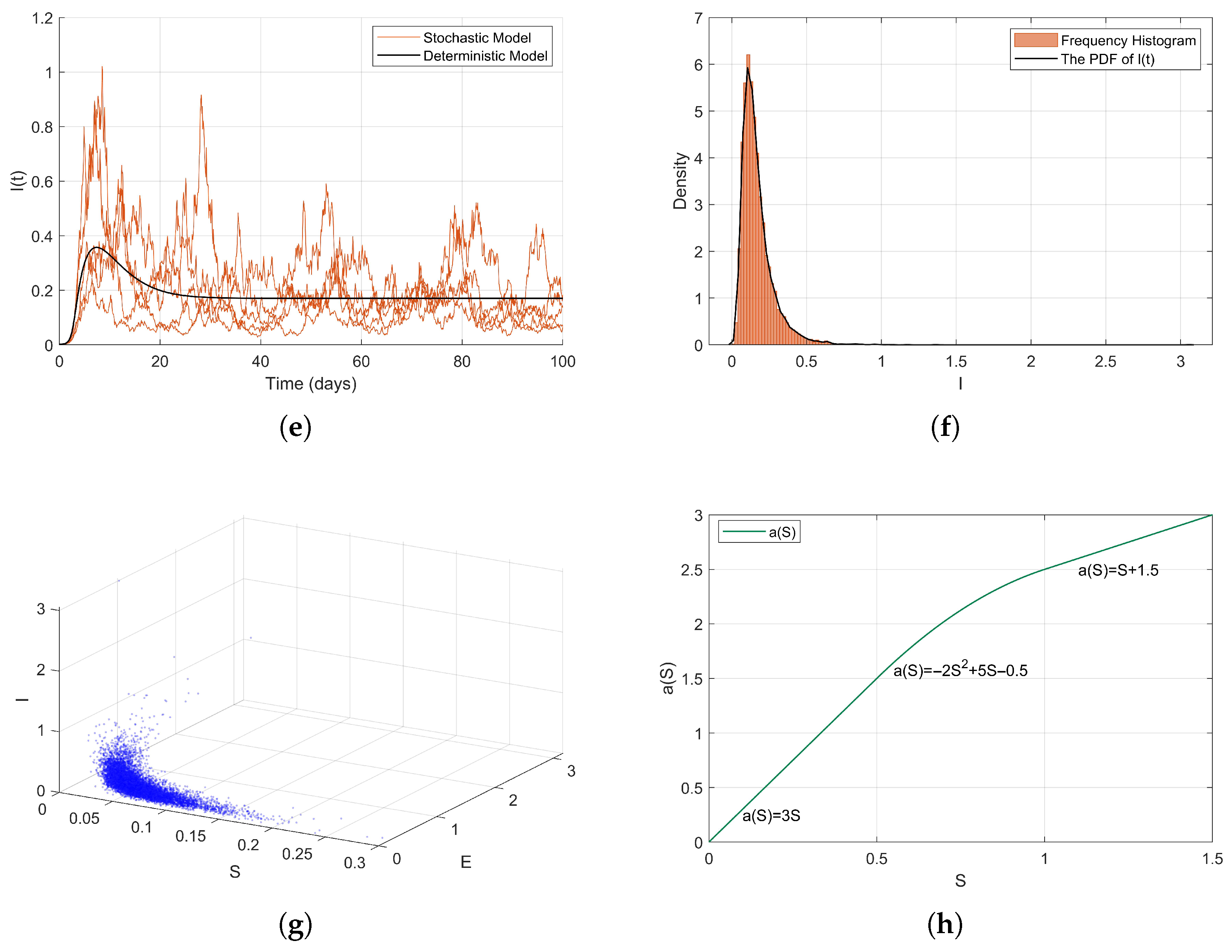
Due to the fact that the state variables of the random model (2) are expected not to tend towards zero, but rather to converge to a non-trivial stationary distribution, where I and E populations maintain positive values, while the S population decreases but is not extinguished, the specific form of the stationary distribution is influenced non-linearly by parameters and the contact rate function $a\left(S\right)$. The concavity and convexity changes of the piecewise function may lead to a multimodal or oscillatory characteristic of the stationary distribution, particularly when S crosses the thresholds of 0.5 and 1.

4. The Existence of Positive Periodic Solutions for Model (3)

In stochastic epidemiological modeling, the investigation of non-trivial positive periodic solutions influenced by seasonal fluctuations or periodic parameters (e.g., time-dependent transmission rates) is crucial for elucidating the long-term dynamics of diseases in time-varying stochastic systems and for designing synchronized control strategies. Consequently, the objective of this section is to rigorously analyze the non-trivial positive periodic solutions of model (3).

For an integrable and bounded function $x\left(t\right)$, define ${\langle g\rangle }_T:=\frac{1}{T}{\int }_0^{T}g\left(t\right)dt$, $x_{\ast }:=\underset{t\in R_{+}}{\inf }x\left(t\right)$ and $x^{\ast }:=\underset{t\in R_{+}}{\sup }x\left(t\right)$.

We first establish the existence and uniqueness of a positive solution for the periodic model, a lemma that is fundamental to subsequent discussions.

Lemma 4.

For any given initial value $X\left(0\right)\in R_{+}^3$, model (3) admits a unique solution $X\left(t\right)$ for $t\ge 0$, and this solution remains in $R_{+}^3$; this is almost certain.

Proof. 

Define the following $C^2$-function $W_1\left(X\left(t\right)\right):R_{+}^3\to R_{+}$

$$W_1\left(X\left(t\right)\right):=\left(S-e_1-e_1\ln \frac{S}{e_1}\right)+(E-1-\ln E)+e_2(I-1-\ln I),$$

(62)

where

$$e_1:=\frac{\left(k_{\ast }+{\mu }_{\ast }\right)\left({\mu }_{\ast }+p_{\ast }+{\gamma }_{\ast }\right)}{M_2^{\circ }\left[{\epsilon }_1\left({\mu }_{\ast }+p_{\ast }+{\gamma }_{\ast }\right)+k^{\ast }\right]},e_2:=\frac{e_1{M}_2^{\circ }}{{\mu }_{\ast }+p_{\ast }+{\gamma }_{\ast }}.$$

(63)

Applying Itô’s formula, we derive

$$d{W}_1=L{W}_{1}dt+{\sigma }_1\left(t\right)\left(S-e_1\right)d{B}_1\left(t\right)+{\sigma }_2\left(t\right)(E-1)d{B}_2\left(t\right)+e_2{\sigma }_3\left(t\right)(I-1)d{B}_3\left(t\right),$$

(64)

where

$$\begin{array}{cc}\hfill L{W}_1=& \Lambda \left(t\right)-a^{\circ }(S,t)\left(I+{\epsilon }_{1}E\right)-\mu \left(t\right)S+\frac{1}{2}{e}_1{\sigma }_1^2+e_1\frac{a^{\circ }(S,t)}{S}\left(I+{\epsilon }_{1}E\right)-e_1\frac{\Lambda \left(t\right)}{S}+e_1\mu \left(t\right)\hfill \\ & +a^{\circ }(S,t)\left(I+{\epsilon }_{1}E\right)-[\mu \left(t\right)+k\left(t\right)]E+\frac{1}{2}{\sigma }_2^2-\frac{a^{\circ }(S,t)}{E}\left(I+{\epsilon }_{1}E\right)+[\mu \left(t\right)+k\left(t\right)]\hfill \\ & +e_{2}k\left(t\right)E-e_2[\mu \left(t\right)+p\left(t\right)+\gamma \left(t\right)]I+\frac{1}{2}{e}_2{\sigma }_3^2-e_{2}k\left(t\right)\frac{E}{I}+e_2[\mu \left(t\right)+p\left(t\right)+\gamma \left(t\right)]\hfill \\ \hfill \le & {\Lambda }^{\ast }+e_1{\mu }^{\ast }+{\mu }^{\ast }+k^{\ast }+\frac{1}{2}{e}_1{\left({\sigma }_1^2\right)}^{\ast }+\frac{1}{2}{\left({\sigma }_2^2\right)}^{\ast }+\frac{1}{2}{e}_2{\left({\sigma }_3^2\right)}^{\ast }+e_2\left({\mu }^{\ast }+p^{\ast }+{\gamma }^{\ast }\right)\hfill \\ & +\left[e_1{M}_2^{\circ }{\epsilon }_1-e_2{k}^{\ast }+\left(k_{\ast }+{\mu }_{\ast }\right)\right]E+\left[e_1{M}_2^{\circ }-e_2\left({\mu }_{\ast }+p_{\ast }+{\gamma }_{\ast }\right)\right]I\hfill \\ \hfill =& {\Lambda }^{\ast }+e_1{\mu }^{\ast }+{\mu }^{\ast }+k^{\ast }+\frac{1}{2}{e}_1{\left({\sigma }_1^2\right)}^{\ast }+\frac{1}{2}{\left({\sigma }_2^2\right)}^{\ast }+\frac{1}{2}{e}_2{\left({\sigma }_3^2\right)}^{\ast }+e_2\left({\mu }^{\ast }+p^{\ast }+{\gamma }^{\ast }\right)\hfill \\ \hfill :=& \mathcal{K},\hfill \end{array}$$

(65)

where $\mathcal{K}$ is a positive constant. The remaining proof follows similarly to Lemma 1. □

Lemma 5.

[41] Suppose that the coefficients involved with model (3) are T-periodic and model (3) owns a unique global solution. Also, there is a function $W(t,x)\in C^2$ in R which is T-periodic in t and satisfies

(B.1) $\underset{\left|x\right|>R}{\inf }W(t,x)\to +\infty$ as $R\to +\infty$.

(B.2) $LW(t,x)\le -1$ outside some compact set.

Then model (3) has a T-periodic solution.

Theorem 3.

If $R_3:=\frac{<\Lambda k{M}_1^{\circ }{>}_T}{{〈\mu +\frac{1}{2}{{\sigma }_1}^2〉}_T{〈\mu +p+\gamma +\frac{1}{2}{{\sigma }_3}^2〉}_T{〈\mu +k+\frac{1}{2}{{\sigma }_3}^2〉}_T}>1$, then the model (3) admits a non-trivial positive periodic solution.

Proof. 

Define the following $C^2$-function $W_2(X\left(t\right),t):[0,+\infty )\times$$R_{+}^3$→$R_{+}$

$$\begin{array}{cc}\hfill W_2(X\left(t\right),t):& =\mathcal{M}\left(-\ln S-v_1\ln E-v_2\ln I-v_{3}I+w\left(t\right)\right)-\ln S-\ln E+\frac{1}{j+1}{(S+E+I)}^{j+1}\hfill \\ \hfill & =\mathcal{M}\left(W_3+w\left(t\right)\right)+W_4+W_5,\hfill \end{array}$$

(66)

where

$$v_1:=\frac{<\Lambda \left(t\right)k\left(t\right)M_1^{\circ }{>}_T}{<\mu \left(t\right)+k\left(t\right)+\frac{1}{2}{\sigma }_2^2\left(t\right){>}_T^2<\mu \left(t\right)+p\left(t\right)+\gamma \left(t\right)+\frac{1}{2}{\sigma }_3^2\left(t\right){>}_T},$$

(67)

$$v_2:=\frac{<\Lambda \left(t\right)k\left(t\right)M_1^{\circ }{>}_T}{<\mu \left(t\right)+k\left(t\right)+\frac{1}{2}{\sigma }_2^2\left(t\right){>}_T<\mu \left(t\right)+p\left(t\right)+\gamma \left(t\right)+\frac{1}{2}{\sigma }_3^2\left(t\right){>}_T^2},v_3:=\frac{M_2^{\circ }{\epsilon }_1}{k_{\ast }},$$

(68)

$$W_3:=-\ln S-v_1\ln E-v_2\ln I-v_{3}I,W_4:=-\ln S-\ln E,W_5:=\frac{1}{j+1}{(S+E+I)}^{j+1},$$

(69)

$j>0$ satisfies $j<\frac{2{\mu }_{\ast }}{{\left({\sigma }_1^2\right)}^{\ast }\vee {\left({\sigma }_2^2\right)}^{\ast }\vee {\left({\sigma }_3^2\right)}^{\ast }}$, $\mathcal{M}>0$ and $\vartheta :=-<\mu +\frac{1}{2}{\sigma }_1^2{>}_T\left(R_v-1\right)$ satisfies $-\vartheta \mathcal{M}+f_2\le -2$, with $R_v$ and $f_2$ to be specified in the proof below.

Let $w^{\prime }\left(t\right):=<R_v{>}_T-R_v\left(t\right)$, integrating the above equation from t to T yields,

$$\begin{array}{cc}\hfill w(t+T)-w\left(t\right)& ={\int }_t^{t+T}{w}^{\prime }\left(s\right)ds={\int }_t^{t+T}\left({〈R_v〉}_T-R_v\left(s\right)\right)ds\hfill \\ \hfill & ={\int }_0^T{R}_v\left(s\right)ds-{\int }_t^{t+T}{R}_v\left(s\right)ds=0.\hfill \end{array}$$

(70)

Thus, $w\left(t\right)$ is a T-periodic function on $[0,+\infty )$. This confirms that $W_2(X\left(t\right),t)$ is also a T-periodic function, and

$$\underset{k\to +\infty ,(S,E,I)\in R_{+}^3\setminus U_k}{\lim }{W}_2(X\left(t\right),t)=+\infty .$$

(71)

This verifies that condition (B.1) in lemma 5 is satisfied. We derive that

$$\begin{array}{cc}\hfill L{W}_3=& -\frac{\Lambda \left(t\right)}{S}+\frac{a^{\circ }(S,t)}{S}\left(I+{\epsilon }_{1}E\right)+\mu \left(t\right)-v_1\frac{a^{\circ }(S,t)}{E}\left(I+{\epsilon }_{1}E\right)+v_1[\mu \left(t\right)+k\left(t\right)]\hfill \\ \hfill & -v_{2}k\left(t\right)\frac{E}{I}+v_2[\mu \left(t\right)+p\left(t\right)+\gamma \left(t\right)]-v_{3}k\left(t\right)E+v_3[\mu \left(t\right)+p\left(t\right)+\gamma \left(t\right)]I\hfill \\ \hfill & +\frac{1}{2}{\sigma }_1^2\left(t\right)+\frac{1}{2}{v}_1{\sigma }_2^2\left(t\right)+\frac{1}{2}{v}_2{\sigma }_3^2\left(t\right)\hfill \\ \hfill \le & v_1\left[\mu \left(t\right)+k\left(t\right)+\frac{1}{2}{\sigma }_2^2\left(t\right)\right]+v_2\left[\mu \left(t\right)+p\left(t\right)+\gamma \left(t\right)+\frac{1}{2}{\sigma }_3^2\left(t\right)\right]+v_3\left({\mu }^{\ast }+p^{\ast }+{\gamma }^{\ast }\right)I\hfill \\ \hfill & +\mu \left(t\right)+\frac{1}{2}{\sigma }_1^2\left(t\right)+M_2^{\circ }I-3\sqrt[3]{v_1{v}_2\Lambda \left(t\right)k\left(t\right)M_1^{\circ }}\hfill \\ \hfill =& R_v\left(t\right)+\left[v_3\left({\mu }^{\ast }+p^{\ast }+{\gamma }^{\ast }\right)+M_2^{\circ }\right]I,\hfill \end{array}$$

(72)

$$L{W}_4\le -\frac{{\Lambda }_{\ast }}{S}+M_2^{\circ }I+M_2^{\circ }{\epsilon }_{1}E-\frac{a^{\circ }(S,t)I}{E}+2{\mu }^{\ast }+k^{\ast }+\frac{1}{2}{\left({\sigma }_1^2\right)}^{\ast }+\frac{1}{2}{\left({\sigma }_2^2\right)}^{\ast },$$

(73)

$$L{W}_5\le -\frac{1}{2}\left[{\mu }_{\ast }-\frac{j}{2}\left({\left({\sigma }_1^2\right)}^{\ast }\vee {\left({\sigma }_2^2\right)}^{\ast }\vee {\left({\sigma }_3^2\right)}^{\ast }\right)\right]\left(S^{j+1}+E^{j+1}+I^{j+1}\right)+J_1,$$

(74)

where

$$R_v\left(t\right):=-3\sqrt[3]{v_1{v}_2\Lambda \left(t\right)k\left(t\right)M_1^{\circ }}+v_1\left[\mu \left(t\right)+k\left(t\right)+\frac{1}{2}{\sigma }_2^2\left(t\right)\right]+v_2\left[\mu \left(t\right)+p\left(t\right)+\gamma \left(t\right)+\frac{1}{2}{\sigma }_3^2\left(t\right)\right]+\mu \left(t\right)+\frac{1}{2}{\sigma }_1^2\left(t\right),$$

(75)

$$J_1:=\underset{(S,E,I)\in {\mathbb{R}}_{+}^3}{\sup }\left\{-\frac{1}{2}\left[{\mu }_{\ast }-\frac{j}{2}\left({\left({\sigma }_1^2\right)}^{\ast }\vee {\left({\sigma }_2^2\right)}^{\ast }\vee {\left({\sigma }_3^2\right)}^{\ast }\right)\right](S^{j+1}+E^{j+1}+I^{j+1})+{\Lambda }^{\ast }{(S+E+I)}^j\right\},$$

(76)

$$\begin{array}{cc}\hfill f_2:=\underset{(S,E,I)\in R_{+}^3}{\sup }& \left\{-\frac{1}{2}\left[{\mu }_{\ast }-\frac{j}{2}\left({\left({\sigma }_1^2\right)}^{\ast }\vee {\left({\sigma }_2^2\right)}^{\ast }\vee {\left({\sigma }_3^2\right)}^{\ast }\right)\right]\left(S^{j+1}+E^{j+1}+I^{j+1}\right)\right.\hfill \\ & \left.+M_2^{\circ }{\epsilon }_{1}E+J_1+2{\mu }^{\ast }+k^{\ast }+\frac{1}{2}{\left({\sigma }_1^2\right)}^{\ast }+\frac{1}{2}{\left({\sigma }_2^2\right)}^{\ast }\right\}.\hfill \end{array}$$

(77)

Thus,

$$\begin{array}{cc}\hfill L\left(W_3+w\left(t\right)\right)& \le <R_v{>}_T+\left[v_3\left({\mu }^{\ast }+p^{\ast }+{\gamma }^{\ast }\right)+M_2^{\circ }\right]I\hfill \\ \hfill & =-<\mu +\frac{1}{2}{\sigma }_1^2{>}_T\left(R_v-1\right)+\left[v_3\left({\mu }^{\ast }+p^{\ast }+{\gamma }^{\ast }\right)+M_2^{\circ }\right]I\hfill \\ \hfill & =-\vartheta +\left[v_3\left({\mu }^{\ast }+p^{\ast }+{\gamma }^{\ast }\right)+M_2^{\circ }\right]I,\hfill \end{array}$$

(78)

$$\begin{array}{cc}\hfill L{W}_2\le & J_1-\frac{1}{2}\left[{\mu }_{\ast }-\frac{j}{2}\left({\left({\sigma }_1^2\right)}^{\ast }\vee {\left({\sigma }_2^2\right)}^{\ast }\vee {\left({\sigma }_3^2\right)}^{\ast }\right)\right]\left(S^{j+1}+E^{j+1}+I^{j+1}\right)-\vartheta \mathcal{M}-\frac{a^{\circ }(S,t)I}{E}\hfill \\ \hfill & +\left\{\mathcal{M}\left[M_2^{\circ }+v_3\left({\mu }^{\ast }+p^{\ast }+{\gamma }^{\ast }\right)\right]+M_2^{\circ }\right\}I+M_2^{\circ }{\epsilon }_{1}E-\frac{{\Lambda }_{\ast }}{S}+2{\mu }^{\ast }+k^{\ast }+\frac{1}{2}{\left({\sigma }_1^2\right)}^{\ast }+\frac{1}{2}{\left({\sigma }_2^2\right)}^{\ast }\hfill \\ \hfill \le & -\vartheta \mathcal{M}-\frac{M_1^{\circ }SI}{E}-\frac{{\Lambda }_{\ast }}{S}+HI+M_2^{\circ }{\epsilon }_{1}E+J_1+2{\mu }^{\ast }+k^{\ast }+\frac{1}{2}{\left({\sigma }_1^2\right)}^{\ast }+\frac{1}{2}{\left({\sigma }_2^2\right)}^{\ast }\hfill \\ \hfill & -\frac{1}{2}\left[{\mu }_{\ast }-\frac{j}{2}\left({\left({\sigma }_1^2\right)}^{\ast }\vee {\left({\sigma }_2^2\right)}^{\ast }\vee {\left({\sigma }_3^2\right)}^{\ast }\right)\right]\left(S^{j+1}+E^{j+1}+I^{j+1}\right).\hfill \end{array}$$

(79)

The remaining proof follows similarly to Theorem 2. □

Numerical Simulations. In this part, we present a numerical example to illustrate the validity of the theoretical results for model (3). The initial values of model (3) are set as $X\left(0\right)=\left(S\right(0),E(0),I(0\left)\right)=(0.995,0.003,0.002)$.

Example 6.

For model (3), we fix the periodic parameters as follows: $\Lambda \left(t\right)=0.05812+0.1sin\pi t,\mu \left(t\right)=0.00003+0.1sin\pi t$, $k\left(t\right)=0.2+0.1sin\pi t$, $p\left(t\right)=0.24+0.1sin\pi t$, $\gamma \left(t\right)=0.1+0.1sin\pi t$, ${\sigma }_1\left(t\right)={\sigma }_2\left(t\right)={\sigma }_3\left(t\right)=0.01+0.05sin\pi t$, ${\epsilon }_1=0.75$, and define the piecewise function $a(S,t)$ as

$$\begin{array}{c}\hfill a^{\circ }(S,t)={\displaystyle \sum _{i=1}^3}{\kappa }_i\left(t\right)f_i\left(S\right)+c_i=\left\{\begin{array}{cc}(3+0.3sin\pi t)S,& 0\le S<0.5,\\ (1.5+0.15sin\pi t)S-0.75,& 0.5\le S<1,\\ (1+0.1sin\pi t)S+1.25,& S\ge 1,\end{array}\right.\end{array}$$

(80)

where $f_1\left(S\right)=3S,f_2\left(S\right)=1.5S,f_3\left(S\right)=1S,c_1=0,c_2=-0.75,c_3=1.25,{\kappa }_i\left(t\right)=1+0.1sin\pi t,i=1,2,3$. The function ${\kappa }_{\mathrm{i}}\left(t\right)$ introduces a time period to simulate seasonal variations in social activities or policy adjustments. The function $f_i\left(S\right)$ defines the contact rate based on different intervals of the susceptible population S, mimicking a tiered control environment. The variable $c_i$ adjusts the baseline of contact rates for each segment, reflecting the impact of policy interventions or environmental factors. Then $M_1^{\circ }=0.32,M_2^{\circ }=2.2,$ $<\Lambda \left(t\right){>}_T=1, <\mu \left(t\right){>}_T=0.2, <k\left(t\right){>}_T=0.5, <p\left(t\right){>}_T=0.15, <\gamma \left(t\right){>}_T=0.25,$ $<{\sigma }_i\left(\mathrm{t}\right){>}_T=0.01$. Then $R_3\approx 1.90>1$. By Theorem 3, model (3) admits a T-periodic solution. This conclusion is visually supported by Figure 8. Furthermore, Figure 8a illustrates that $\mathrm{S}\left(\mathrm{t}\right),\mathrm{E}\left(\mathrm{t}\right)$, and $\mathrm{I}\left(\mathrm{t}\right)$ exhibit sustained periodic oscillations, confirming the existence of a non-trivial periodic regime under stochastic perturbations.

The cyclical model reveals the amplifying effect of temporal factors on the spread of COVID-19, emphasizing the importance of holiday or seasonal interventions. The simulation figures highlight the peaks of temporal transmission and the effects of tiered control measures, suggesting the adoption of dynamic and targeted intervention strategies to manage periodic risks.

5. Conclusions

Building on an extended stochastic semi-parametric SEIR model with latent periods (model (1)), this study examines a three-dimensional model (model (2)) and a periodic stochastic model (model (3)), analyzing strong disease persistence, stationary distribution, and periodic solutions through numerical simulations of $a\left(S\right(t\left)\right)$ and $a^{\circ }(S,t)$ using linear, piecewise, and piecewise smooth functions. Key findings indicate that $R_2=\frac{k\Lambda M_1}{\left(\mu +\frac{1}{2}{\sigma }_1^2\right)\left(\mu +k+\frac{1}{2}{\sigma }_2^2\right)\left(\mu +p+\gamma +\frac{1}{2}{\sigma }_3^2\right)}>1$ ensures disease persistence and a stationary distribution in model (2), while $R_3=\frac{{〈k\Lambda M_1^{\circ }〉}_T}{{〈\mu +\frac{1}{2}{\sigma }_1^2〉}_T{〈\mu +p+\gamma +\frac{1}{2}{\sigma }_3^2〉}_T{〈\mu +k+\frac{1}{2}{\sigma }_3^2〉}_T}>1$ guarantees positive periodic solutions in model (3). Compared to the deterministic model’s basic reproduction number $R_0=\frac{\left(k+{\epsilon }_1(\mu +p+\gamma )\right)a\left(\frac{\Lambda }{\mu }\right)}{(\mu +k)(\mu +p+\gamma )},R_2\le R_0$ without disturbance in model (2) and $R_3\le R_0$ without periodicity in model (3), underscoring the impact of stochastic noise and periodic factors on disease dynamics.

References

1. Allen, L.J.S. Some discrete-time SI, SIR, and SIS epidemic models. Math. Biosci. 1994, 124, 83–105. [Google Scholar] [CrossRef] [PubMed]
2. Li, J.; Ma, Z. Global analysis of SIS epidemic models with variable total population size. Math. Comput. Model. 2004, 39, 1231–1242. [Google Scholar] [CrossRef]
3. Corteel, M. Shaping epidemic dynamics: An historical epistemology study of the SIR model. Hist. Hum. Sci. 2025, 09526951251317104. [Google Scholar] [CrossRef]
4. Jin, Y.; Wang, W.; Xiao, S. An SIRS model with a nonlinear incidence rate. Chaos Solitons Fractals 2007, 34, 1482–1497. [Google Scholar] [CrossRef]
5. Li, M.Y.; Muldowney, J.S. Global stability for the SEIR model in epidemiology. Math. Biosci. 1995, 125, 155–164. [Google Scholar] [CrossRef] [PubMed]
6. Zhang, T.; Teng, Z. On a nonautonomous SEIRS model in epidemiology. Bull. Math. Biol. 2007, 69, 2537–2559. [Google Scholar] [CrossRef] [PubMed]
7. d’Onofrio, A. Stability properties of pulse vaccination strategy in SEIR epidemic model. Math. Biosci. 2002, 179, 57–72. [Google Scholar] [CrossRef] [PubMed]
8. Zhao, Z.; Chen, L.; Song, X. Impulsive vaccination of SEIR epidemic model with time delay and nonlinear incidence rate. Math. Comput. Simul. 2008, 79, 500–510. [Google Scholar] [CrossRef]
9. Pang, L.; Ruan, S.; Liu, S.; Zhao, Z.; Zhang, X. Transmission dynamics and optimal control of measles epidemics. Appl. Math. Comput. 2015, 256, 131–147. [Google Scholar] [CrossRef]
10. Abdelaziz, M.A.M.; Ismail, A.I.; Abdullah, F.A.; Mohd, M.H. Codimension one and two bifurcations of a discrete-time fractional-order SEIR measles epidemic model with constant vaccination. Chaos Solitons Fractals 2020, 140, 110104. [Google Scholar] [CrossRef]
11. Jiao, J.; Liu, Z.; Cai, S. Dynamics of an SEIR model with infectivity in incubation period and homestead-isolation on the susceptible. Appl. Math. Lett. 2020, 107, 106442. [Google Scholar] [CrossRef] [PubMed]
12. Mishra, A.M.; Purohit, S.D.; Owolabi, K.M.; Sharma, Y.D. A nonlinear epidemiological model considering asymptotic and quarantine classes for SARS CoV-2 virus. Chaos Solitons Fractals 2020, 138, 109953. [Google Scholar] [CrossRef] [PubMed]
13. Amaral, M.A.; de Oliveira, M.M.; Javarone, M.A. An epidemiological model with voluntary quarantine strategies governed by evolutionary game dynamics. Chaos Solitons Fractals 2021, 143, 110616. [Google Scholar] [CrossRef] [PubMed]
14. Meng, L.; Zhu, W. Analysis of SEIR epidemic patch model with nonlinear incidence rate, vaccination and quarantine strategies. Math. Comput. Simul. 2022, 200, 489–503. [Google Scholar] [CrossRef]
15. Khan, M.M.; Arefin, M.R.; Tanimoto, J. Investigating the trade-off between self-quarantine and forced quarantine provisions to control an epidemic: An evolutionary approach. Appl. Math. Comput. 2022, 432, 127365. [Google Scholar] [CrossRef] [PubMed]
16. Fan, X.; Wang, Z. Stability analysis of an SEIR epidemic model with stochastic perturbation and numerical simulation. Int. J. Nonlinear Sci. Numer. Simul. 2013, 14, 113–121. [Google Scholar] [CrossRef]
17. Liu, Q.; Jiang, D.; Shi, N.; Hayat, T.; Ahmad, B. Stationary distribution and extinction of a stochastic SEIR epidemic model with standard incidence. Phys. A 2017, 476, 58–69. [Google Scholar] [CrossRef]
18. Shangguan, D.; Liu, Z.; Wang, L.; Tan, R. A stochastic epidemic model with infectivity in incubation period and homestead–isolation on the susceptible. J. Appl. Math. Comput. 2021, 67, 785–805. [Google Scholar] [CrossRef] [PubMed]
19. Liu, Q.; Jiang, D. Stationary distribution and probability density for a stochastic SEIR-type model of coronavirus (COVID-19) with asymptomatic carriers. Chaos Solitons Fractals 2023, 169, 113256. [Google Scholar] [CrossRef] [PubMed]
20. Saha, P.; Pal, K.K.; Ghosh, U.; Tiwari, P.K. Dynamic analysis of deterministic and stochastic SEIR models incorporating the Ornstein–Uhlenbeck process. Chaos 2025, 35, 023165. [Google Scholar] [CrossRef] [PubMed]
21. Liu, W.; Hethcote, H.W.; Levin, S.A. Dynamical behavior of epidemiological models with nonlinear incidence rates. J. Math. Biol. 1987, 25, 359–380. [Google Scholar] [CrossRef] [PubMed]
22. Korobeinikov, A.; Maini, P.K. A Lyapunov function and global properties for SIR and SEIR epidemiological models with nonlinear incidence. Math. Biosci. Eng. 2004, 1, 57–60. [Google Scholar] [CrossRef] [PubMed]
23. Biswas, M.H.A.; Paiva, L.T.; De Pinho, M.D.R. A SEIR model for control of infectious diseases with constraints. Math. Biosci. Eng. 2014, 11, 761–784. [Google Scholar] [CrossRef]
24. Piccirillo, V. Nonlinear control of infection spread based on a deterministic SEIR model. Chaos Solitons Fractals 2021, 149, 111051. [Google Scholar] [CrossRef] [PubMed]
25. Huang, L.; Xia, Y.; Qin, W. Study on SEAI model of COVID-19 based on asymptomatic infection. Axioms 2024, 13, 309. [Google Scholar] [CrossRef]
26. Xu, S.; Hu, Y. Dynamic analysis of a Caputo fractional-order SEIR model with a general incidence rate. Sci. Rep. 2025, 15, 17561. [Google Scholar] [CrossRef] [PubMed]
27. Liu, Q.; Jiang, D.; Shi, N.; Hayat, T.; Alsaedi, A. Asymptotic behavior of a stochastic delayed SEIR epidemic model with nonlinear incidence. Phys. A 2016, 462, 870–882. [Google Scholar] [CrossRef]
28. Upadhyay, R.K.; Pal, A.K.; Kumari, S.; Roy, P. Dynamics of an SEIR epidemic model with nonlinear incidence and treatment rates. Nonlinear Dyn. 2019, 96, 2351–2368. [Google Scholar] [CrossRef]
29. Zhang, J.; Jin, T. A stochastic semi-parametric SEIR model with infectivity in an incubation period. Mathematics 2024, 12, 1580. [Google Scholar] [CrossRef]
30. Ain, Q.T.; Qiang, X.; Rao, Y.; Shi, X.; Kosari, S.; Kou, Z. Extinction dynamics and equilibrium patterns in stochastic epidemic model for norovirus: Role of temporal immunity and generalized incidence rates. Fractal Fract. 2024, 8, 586. [Google Scholar] [CrossRef]
31. Gouriéroux, C.; Lu, Y. Susceptible-infected-recovered model with stochastic transmission. Can. J. Stat. 2025, 53, e11835. [Google Scholar] [CrossRef]
32. Liu, X.; Cao, H.; Nie, L. Insights into infectious diseases with horizontal and environmental transmission: A stochastic model with logarithmic Ornstein–Uhlenbeck process and nonlinear incidence. Chaos Solitons Fractals 2025, 191, 115888. [Google Scholar] [CrossRef]
33. Zhao, D.; Duan, J.; Liu, R.; Guo, K. Dynamic analysis of a stochastic microorganism flocculation model with two complementary nutrients and nonlinear perturbation. Adv. Contin. Discrete Models 2025, 2025, 37. [Google Scholar] [CrossRef]
34. Hethcote, H.W.; Levin, S.A. Periodicity in epidemiological models. In Applied Mathematical Ecology; Springer: Berlin/Heidelberg, Germany, 1989; pp. 193–211. [Google Scholar] [CrossRef]
35. Kuznetsov, Y.A.; Piccardi, C. Bifurcation analysis of periodic SEIR and SIR epidemic models. J. Math. Biol. 1994, 32, 109–121. [Google Scholar] [CrossRef] [PubMed]
36. Nakata, Y.; Kuniya, T. Global dynamics of a class of SEIRS epidemic models in a periodic environment. J. Math. Anal. Appl. 2010, 363, 230–237. [Google Scholar] [CrossRef]
37. Li, F.; Zhao, X.Q. A periodic SEIRS epidemic model with a time-dependent latent period. J. Math. Biol. 2019, 78, 1553–1579. [Google Scholar] [CrossRef] [PubMed]
38. Shangguan, D.; Liu, Z.; Wang, L.; Tan, R. Periodicity and stationary distribution of two novel stochastic epidemic models with infectivity in the latent period and household quarantine. J. Appl. Math. Comput. 2022, 68, 2551–2570. [Google Scholar] [CrossRef] [PubMed]
39. Zhao, L.; Liu, Y. Time periodic traveling wave solutions of a time-periodic reaction–diffusion SEIR epidemic model with periodic recruitment. Nonlinear Anal. Real World Appl. 2025, 81, 104167. [Google Scholar] [CrossRef]
40. Mao, X.R. Stochastic Differential Equations and Their Applications; Horwood: Chichester, UK, 1997. [Google Scholar]
41. Khasminskii, R. Stochastic Stability of Differential Equations; Springer: Berlin/Heidelberg, Germany, 2011; Volume 66. [Google Scholar] [CrossRef]
Figure 1. Diagram of the deterministic model of model (1).
Axioms 14 00535 g001
Figure 2. (a) Temporal dynamics of the SEI state variables in the stochastic model (2). (b) Linear function a ( S ) and its relationship with S.
Axioms 14 00535 g002
Figure 3. (a) Temporal dynamics of the SEI state variables in the stochastic model (2). (b) Piecewise linear function a ( S ) and its relationship with S.
Axioms 14 00535 g003
Figure 4. (a) Temporal dynamics of the SEI state variables in the stochastic model (2). (b) Monotonically increasing smooth convex function a ( S ) and its relationship with S.
Axioms 14 00535 g004
Figure 5. (a) Temporal dynamics of the SEI state variables in the stochastic model (2). (b) Monotonically increasing smooth concave function a ( S ) and its relationship with S.
Axioms 14 00535 g005
Figure 6. (a) Temporal dynamics of the SEI state variables in the stochastic model (2). (b) Logarithmic function function a ( S ) and its relationship with S.
Axioms 14 00535 g006
Figure 7. (a) Susceptible population dynamics. (b) Stationary distribution of S(t). (c) Exposed population dynamics. (d) Stationary distribution of E(t). (e) Infected population dynamics. (f) Stationary distribution of I(t). (g) Joint stationary distribution. (h) Monotonically increasing smooth curvex function a ( S ) and its relationship with S.
Axioms 14 00535 g007aAxioms 14 00535 g007b
Figure 8. (a) Temporal dynamics of SEI state variables in the stochastic periodic model. (b) Time-dependent profile of a ( S , t ) as a function of t. (c) Dependence of a ( S , t ) on S at a fixed time t = 0 .
Axioms 14 00535 g008