Transfer Learning of High-Dimensional Stochastic Frontier Model via Elastic Net

Abstract

In this paper, the high-dimensional stochastic frontier model problem is explored via Elastic Net under the transfer learning framework. When the target data is limited, transfer learning improves the accuracy of model estimation and prediction by transferring the source data. When the transferable source is known, a transfer learning algorithm for a high-dimensional stochastic frontier model is proposed based on Elastic Net. In addition, based on the prior knowledge of the parameters, this paper introduces linear constraints to improve the estimation accuracy in transfer learning. When the transferable source is unknown, this paper designs a corresponding algorithm to detect the transferable source. Finally, the effectiveness of the method is proved by simulation experiments and actual cases.

1. Introduction

Efficiency analysis is one of the main methods of studying economic growth rate and determining the causes of economic growth. Stochastic frontier analysis is a common method of efficiency analysis, which is widely used in economics, management, and other fields. Aigner et al. [1], Meeusen and Broeck [2] and Battese and Corra [3] have proposed the stochastic frontier analysis (SFA), which is based on the deterministic production frontier model proposed by Aigner and Chu [4], and adds a random error term (denoted as v) so that the frontier production function also has randomness. It is usually assumed that this error term is an ordinary white noise error term and obeys a normal distribution. Generally, u is used to represent the technical inefficiency term, assuming that it is non-negative and independent of v. The stochastic frontier function can be expressed as $f(X;\beta )·exp(v-u)$, where $f\left(X\right)$ denotes the functional form of the production function, typically specified as a Cobb–Douglas function.

The most obvious difference between the stochastic frontier model and the general econometric model is that there is a composite error term $v-u$. In order to estimate the parameters contained in the error term and calculate the technical efficiency, it is necessary to make more detailed assumptions on the distribution of the error term. Battese and Corra [3] assume that u obeys a half normal distribution, which is the most commonly adopted assumption in stochastic frontier models. Meeusen and Broeck [2] assume that u obeys exponential distribution, which has good properties and is often used. Greene [5,6] proposes the Gamma distribution hypothesis of the inefficiency term u, but it has been questioned. Stevenson [7] proposes the truncated normal distribution assumption of u. In our paper, the most commonly used half normal distribution hypothesis is used for model estimation. Stochastic frontier analysis is a common method for efficiency measurement. After a long period of development, a series of theoretical innovations on stochastic frontier model setting and estimation and technical efficiency estimation and inference have emerged.

In the era of big data, data sets are often massive and diverse. However, in practical applications, the amount of data collected or generated by people is often not enough to provide accurate models for estimation and prediction. For example, when using stochastic frontier analysis to analyze the production efficiency of production units, the analysis performance depends on a large amount of labeled data, but obtaining sufficient labeled data to train the model is usually expensive and time-consuming. Moreover, the data collected or generated by people generally exist in high-dimensional form, so using stochastic frontier analysis requires us to consider the problem that the amount of data is too small and the data is high-dimensional.

In order to solve the problem that the amount of data is too small, researchers have begun to consider integrating different but related data sets to improve the accuracy of parameter estimation and prediction. The idea of transfer learning is to find relevant data sets from existing domains and reduce data set bias by learning in new target domains. So far, transfer learning has been widely used in various fields such as computer science [8], health care [9] and power security [10], which fully proves the effectiveness of transfer learning.

High-dimensional data analysis has attracted people’s attention for a long time in the past, and many effective methods have been proposed. The Elastic Net developed by Zou and Hastie [11] is a very efficient and practical method. Elastic Net is a hybrid regularization technique that has gained significant attention due to its remarkable ability to handle high-dimensional data, address collinearity, and select relevant features. In addition, Jia and Yu [12] and Yuan and Lin [13] establish the theoretical properties of the Elastic Net, such as statistical consistency and convergence rate, which provided a solid foundation for its practical application. Similar to transfer learning, high-dimensional data analysis often encounters the challenge of limited sample size, where the number of samples is significantly smaller than the data dimension. Therefore, people began to apply transfer learning to high-dimensional problems.

In order to achieve this goal, Bastani [14] adopts transfer learning in the context of high-dimensional problems, mainly focusing on estimation and prediction in high-dimensional linear models. Following the traditional framework of transfer learning, Bastani [14] operates under the assumption that there is a certain degree of similarity between the target model and the source model. If the similarity condition is violated, negative transfer may occur, which means that the increase in sample size will actually lead to worse training and prediction results of the model. Notably, Bastani [14] assumes that the objective model is high-dimensional, while ensuring that the size of the source data is much larger than the dimension. In addition, the study only considers a single source model and does not explore scenarios involving multiple sources. As a way of further improvement, Li et al. [15] consider multiple sources, with both the source and target models situated in high-dimensional settings. Based on the work of Li et al. [15,16], the concept of transfer learning is extended to high-dimensional generalized linear models. They introduce an algorithm-free method to identify transferable sources in the source detection context, and always select transferable sources to prevent negative transfer.

Building on the research of Bastani [14] and Li et al. [15], Meng et al. [17] introduce a novel two-step transfer learning algorithm for cases where the transferable domain is known. This algorithm employs the Elastic Net penalty in both the transfer and debiasing steps. In addition, when the transferable source is unknown, a new algorithm for detecting the transferable source through the Elastic Net is also proposed. Furthermore, based on the high-dimensional model, Chen et al. [18] add the constraints of prior knowledge and study robust transfer learning. Finally, through experiments, it is proved that it is feasible to use transfer learning for high-dimensional models with linear constraints, and the performance of the model is greatly improved. When the transferable source is unknown, a constrained transferable source detection algorithm is proposed. The above high-dimensional problems are mostly based on linear regression models. For high-dimensional stochastic frontier models, Qingchuan and Shichuan [19] pioneered the use of the Alasso penalty method to select variables in stochastic frontier models, and achieved good results.

As far as we know, no one has applied the Elastic Net to the stochastic frontier model. Inspired by the work of Meng et al. [17] and Qingchuan and Shichuan [19], we explore the use of the Elastic Net in high-dimensional stochastic frontier models to perform variable selection and address multicollinearity issues, and further apply this approach in a transfer learning framework. To enhance the accuracy of coefficient estimation and improve overall model performance, we are additionally inspired by Chen et al. [18]. According to the prior knowledge, we add equality and inequality constraints to limit the coefficient estimation to a certain range.

This paper proposes transfer learning of high-dimensional stochastic frontier model via Elastic Net. To improve the accuracy of coefficient estimation and enhance model performance, inspired by Chen et al. [18], we incorporate equality and inequality constraints based on prior knowledge to restrict the coefficient estimates within a certain range. The following are the innovations of this paper:

(1)

When the transferable source domain is known, we propose a high-dimensional stochastic frontier transfer learning algorithm via Elastic Net.

(2)

When the transferable source domain is unknown, we design a transferable source detection algorithm.

(3)

When some prior knowledge is known, we add linear constraints to the model so that the coefficient estimation is reduced to a certain range and the coefficient estimation is improved.

The rest of this paper is organized as follows. In Section 1, we first briefly review the stochastic frontier model and transfer learning. Then we introduce the Elastic Net stochastic frontier model with transfer learning based on known transferable sources and unknown transferable sources in Section 2. Next, we perform extensive simulations in Section 3 and one real data experiment in Section 4. Finally, we summarize our paper in Section 5.

2. Methodology

2.1. High-Dimensional Stochastic Frontier Model via Elastic Net

This paper studies the following stochastic frontier models

$$Y=f(X;\beta )·exp(v-u),$$

(1)

where $f(X;\beta )$ represents the frontier production function, v is the bilateral random error term, and u represents the technical inefficiency term. Formula (1) uses the Cobb–Douglas production function. The stochastic frontier model based on Cobb–Douglas production function and logarithm is

$$lnY={\beta }_0+\sum {\beta }_{k}lnX+v-u.$$

(2)

For the sake of convenience, let $x=lnX$ and $y=lnY$, then the Formula (2) can be expressed as

$$y=x\beta +v-u,$$

(3)

where $v\sim N(0,{\sigma }_v^2)$ and $u\sim N^{+}(0,{\sigma }_u^2)$.

Although Formula (3) is similar to the ordinary linear model, the perturbation term $\epsilon =v-u$ is asymmetric due to the introduction of the non-negative term u. This asymmetry allows for the identification of the existence and distribution of u. We assume that $v\sim \mathcal{N}(0,{\sigma }_v^2)$, $u\sim {\mathcal{N}}^{+}(0,{\sigma }_u^2)$, and that v and u are mutually independent and also independent of the explanatory variables. Based on these assumptions, the log-likelihood function can be derived as follows [20]:

$$lnL(\epsilon \mid \lambda ,{\sigma }^2)=nln\left({\displaystyle \frac{\sqrt{2}}{\sqrt{\pi }}}\right)+nln\left({\displaystyle \frac{1}{\sigma }}\right)+\sum _{i=1}^{n}ln\left[1-\mathrm{\Phi }\left({\epsilon }_i\lambda {\sigma }^{-1}\right)\right]-{\displaystyle \frac{1}{2{\sigma }^2}}\sum _{i=1}^n{\epsilon }_i^2,$$

(4)

where ${\epsilon }_i=y_i-x_i\beta$, ${\sigma }^2={\sigma }_u^2+{\sigma }_v^2$, and $\lambda ={\sigma }_u/{\sigma }_v$. The function $\mathrm{\Phi }(·)$ denotes the cumulative distribution function of the standard normal distribution.

Compared with the ordinary linear model, the log-likelihood function in Formula (4) introduces a nonlinear term to reflect the presence of inefficiency. Ordinary linear models typically assume that the error term follows a symmetric normal distribution, and their likelihood functions involve only the exponential of the squared residuals. In stochastic frontier models, however, the residual is decomposed into white noise and an inefficiency term, which is assumed to follow a half-normal distribution. Consequently, Formula (4) includes the nonlinear term $ln[1-\mathrm{\Phi }({\epsilon }_i\lambda /\sigma )]$, which characterizes the asymmetry in the residual distribution.

This difference has an important influence on the optimization process. First, the likelihood function no longer has a closed-form solution, requiring numerical methods for parameter estimation. Second, the nonlinear term may lead to numerical instability—especially when $\mathrm{\Phi }(·)$ approaches 1, causing $1-\mathrm{\Phi }(·)$ to become nearly zero, which results in a loss of precision in the logarithmic term. Therefore, stabilization techniques are necessary in practical optimization. Finally, the inclusion of the additional parameters $\lambda$ and $\sigma$ increases the dimensionality of the optimization problem, making the estimation process more complex.

In general, we use maximum likelihood estimation for parameter estimation but typically do not account for cases where the number of features exceeds the number of samples. To this end, we add regularization terms to achieve feature selection and address the collinearity problem. For convenience, we define $ln{L}_i$ as the negative log-likelihood function for the i-th observation. The resulting optimization problem can be expressed as

$$\underset{\beta }{min}\sum _{i=1}^{n}ln{L}_i\left(\beta \right)+{\lambda }_1{\parallel \beta \parallel }_1+{\lambda }_2{\parallel \beta \parallel }_2^2.$$

(5)

If we have some prior knowledge of the parameters before the estimation, we can incorporate linear equality and inequality constraints. This transforms Formula (5) into the following constrained optimization problem:

$$\underset{\beta }{min}\sum _{i=1}^{n}ln{L}_i\left(\beta \right)+{\lambda }_1{\parallel \beta \parallel }_1+{\lambda }_2{\parallel \beta \parallel }_2^{2}s.t.C\beta \ge d,E\beta =f.$$

(6)

Among them, ${\lambda }_1$ and ${\lambda }_2$ are the penalty parameters, and $C\in R^{q\times p},d\in R^q,E\in R^{m\times p},f\in R^m$ are vectors that are set according to the actual situation. The Formula (5) can be used to select parameters by ${\lambda }_1{\parallel \beta \parallel }_1$, and the collinearity problem can be solved by ${\lambda }_2{\parallel \beta \parallel }_2^2$.

We now provide a more detailed introduction to the linear constraints to enhance readability. If we know some prior knowledge of the parameters before the estimation, such as ${\beta }_1\ge a$, $w{\beta }_2+v{\beta }_3\ge b$ and ${\beta }_4=c$, where $w,v,a,b,c$ is a real number, then we can use this knowledge to construct a linear constraint. Specifically, the following matrix is constructed:

$$C=\left[\begin{array}{cccccc}1& 0& 0& 0& \dots & 0\\ 0& w& v& 0& \dots & 0\\ ⋮& ⋮& ⋮& ⋮& \ddots & ⋮\\ 0& 0& 0& 0& \dots & 0\end{array}\right]\in {\mathbb{R}}^{q\times p},d=\left[\begin{array}{c}a\\ b\\ ⋮\\ 0\end{array}\right]\in {\mathbb{R}}^{q\times 1}$$

$$E=\left[\begin{array}{cccccc}0& 0& 0& 1& \dots & 0\\ 0& 0& 0& 0& \dots & 0\\ ⋮& ⋮& ⋮& ⋮& \ddots & ⋮\\ 0& 0& 0& 0& \dots & 0\end{array}\right]\in {\mathbb{R}}^{q\times p},f=\left[\begin{array}{c}c\\ 0\\ ⋮\\ 0\end{array}\right]\in {\mathbb{R}}^{q\times 1}$$

The inequality constraint is $C\beta \ge d$, and the equality constraint is $E\beta =f$.

Here, we discuss the linear constraints derived from prior knowledge and the regularization terms ${\lambda }_1{\parallel \beta \parallel }_1$ and ${\lambda }_2{\parallel \beta \parallel }_2^2$. The regularization terms are considered soft constraints, which influence the objective function through penalty terms, thereby contributing to structural selection and preventing overfitting during model training. In contrast, linear constraints are hard constraints that typically originate from domain-specific prior knowledge. While regularization helps control model complexity and enhance interpretability, linear constraints enforce parameter feasibility based on the actual problem setting. The two types of constraints are complementary in nature.

In addition, to solve the optimization problem in Formula (6), we refer to the framework proposed by Zou et al. [11] and introduce several modifications. First, the Elastic Net penalty term in the original problem is equivalently reformulated as a standard Lasso problem. Following Lemma 1 in Zou et al. [11], an extended data set is constructed to achieve this transformation. As a result, the original problem is converted into a minimization problem with an ${\ell }_1$ penalty. The Lasso solution path is then computed on the extended data set using a standard Lasso algorithm, and the final solution to the original problem is recovered through variable transformation.

The choice of penalty parameters has a significant impact on the estimation. Here, we take the Formula (5) as an example to briefly illustrate the selection of the penalty parameters ${\lambda }_1$ and ${\lambda }_2$. The same strategy can be applied to determine the penalty parameters in other parts of the model.

By introducing the mixing parameter $\lambda$, the optimization problem becomes

$$\underset{\beta }{min}\sum _{i=1}^{n}ln{L}_i\left(\beta \right)+\alpha \lambda {\parallel \beta \parallel }_1+{\displaystyle \frac{1-\alpha }{2}}\lambda {\parallel \beta \parallel }_2^2,$$

(7)

where $\lambda ={\lambda }_1+{\lambda }_2$ and $\alpha \in [0,1]$. Given a fixed $\alpha$ and a sequence candidate values ${\lambda }^1,\dots ,{\lambda }^m$, we use five-fold cross validation to find the optimal $\lambda$. The process involves randomly dividing the sample data into five subsets, using one subset as the validation set and the remaining subsets as the training set for each iteration. For each candidate value ${\lambda }^{\ell }$ ($\ell =1,\dots ,m$), the model is trained on the training set and evaluated on the validation set. The value of $\lambda$ that minimizes the mean absolute error ($MAE$) across all validation sets is selected as the final penalty parameter.

When the sample size of the target data is large, the above constraint variable selection method has achieved good results, but when the sample size of the target data is small, the variable selection effect is not ideal. In this case, it is necessary to use transfer learning technology to transfer data from similar distributed source data sets.

2.2. Transfer Learning of High-Dimensional Stochastic Frontier Model via Elastic Net

Transfer learning usually has two domains: source domain and target domain, respectively. The target domain, which has limited data or labels, is the focus of learning, while the source domain contains abundant data or rich label information. Although the source and target domains may differ in data distribution, they share certain similarities. The purpose of transfer learning is to transfer knowledge from the source domain to the target domain to complete model learning.

Suppose that the target data $(X^{\left(0\right)},Y^{\left(0\right)})$, where the ith target data is defined as $(x_i^{\left(0\right)},y_i^{\left(0\right)})$, comes from the following stochastic frontier model

$$y_i^{\left(0\right)}=x_i^{\left(0\right)}\beta +v_i^{\left(0\right)}-u_i^{\left(0\right)},i=1,2,3,\dots ,n.$$

(8)

Then the target model is constructed:

$$\sum ln{L}_i\left(\beta \right)+{\lambda }_1{\parallel \beta \parallel }_1+{\lambda }_2{\parallel \beta \parallel }_2^2.$$

(9)

Assume that there are K source data sets $(X^{\left(K\right)},Y^{\left(K\right)})$. And the kth source data set is represented as $(X^{\left(k\right)},Y^{\left(k\right)})$, where $X_{\left(k\right)}\in R^{n_k\times p}$ and $Y^{\left(k\right)}\in R^{n_k}$. The kth source data set of the jth data is represented as $(x_j^{\left(k\right)},y_j^{\left(k\right)})$. The source data comes from the stochastic frontier model:

$$y_j^{\left(k\right)}=x_j^{\left(k\right)}{w}^{\left(k\right)}+v_j^{\left(k\right)}-u_j^{\left(k\right)},j=1,2,3,\dots ,n_k.$$

(10)

In this paper, we refer to source data sets that meet a predefined similarity condition as transferable sources. Only the information from these transferable sources is utilized to enhance the coefficient estimation for the target data. This restriction is reasonable, as it ensures that the incorporated information is sufficiently relevant and consistent with the target domain, thereby improving the accuracy and robustness of the estimation. In contrast, if the similarity between the source and target domains is insufficient, incorporating source data may degrade performance rather than improve it.

We now define a transferable source. Given any positive threshold $h>0$, let $\beta =w^{\left(0\right)}$ denote the parameter vector of the target model, and let $w^{\left(k\right)}$ denote the parameter vector of the kth source model. Define the difference as ${\delta }^{\left(k\right)}=\beta -w^{\left(k\right)}$. If ${\parallel {\delta }^{\left(k\right)}\parallel }_1\le h$, the k-th source is considered transferable. The index set of all transferable sources is then defined as $\mathcal{A}=\left\{k:{\parallel {\delta }^{\left(k\right)}\parallel }_1\le h\right\}$.

This paper studies how to perform transfer learning on high-dimensional stochastic frontier models with known and unknown transferable sources, and how to perform transfer learning on high-dimensional stochastic frontier models with linear constraints.

2.2.1. Known Transferable Sources and No Constraints

Suppose there is a set of transferable sources ${\mathcal{A}}_h$, where the sample size is $n_{\mathcal{A}}$. Firstly, the target data and transferable data are brought into the log-likelihood function with regularization term to obtain ${\widehat{w}}^{\mathcal{A}}$

$${\widehat{w}}^{\mathcal{A}}\leftarrow arg\underset{w}{min}\left\{\sum _{i=1}^{n_0+n_{\mathcal{A}}}ln{L}_i\left(\widehat{w}\right)+{\lambda }_1{\parallel w\parallel }_1+{\lambda }_2{\parallel w\parallel }_2^2\right\},$$

(11)

where ${\epsilon }_i=y_i-x_i\widehat{w}$.

Next, the target data is brought into the log-likelihood function with regularization term to obtain ${\widehat{\delta }}_{\mathcal{A}}$

$${\widehat{\delta }}^{\mathcal{A}}\leftarrow arg\underset{\delta }{min}\left\{\sum _{i=1}^{n_0}ln{L}_i({\widehat{w}}^{\mathcal{A}}+\delta )+{\eta }_1{\parallel \delta \parallel }_1+{\eta }_2{\parallel \delta \parallel }_2^2\right\},$$

(12)

where ${\epsilon }_i=y_i-x_i({\widehat{w}}^{\mathcal{A}}+\delta )$.

The penalty parameters ${\lambda }_1$, ${\lambda }_2$, ${\eta }_1$ and ${\eta }_2$ are obtained by cross validation. In order to help readers easily understand the algorithm, the $\mathcal{A}$-Trans algorithm is shown in Algorithm 1.

The transfer learning algorithm proposed below is an improvement of the two-step transfer learning framework introduced by Chen et al. [18]. The main difference lies in the use of a different likelihood function. The practicability and effectiveness of the original algorithm have been demonstrated in their paper.    

Algorithm 1: $\mathcal{A}$-Trans

Input: Target data $(X^{\left(0\right)},Y^{\left(0\right)})$, transferable source data ${\left\{(X^{\left(k\right)},Y^{\left(k\right)})\right\}}_{k=1}^K$, penalty parameter ${\lambda }_1$, ${\lambda }_2$, ${\eta }_1$ and ${\eta }_2$    Output: The estimated coefficient vector $\widehat{\beta }$ 1 Transferring step: $${\widehat{w}}^{\mathcal{A}}\leftarrow arg\underset{w}{min}\left\{\sum _{i=1}^{n_0+n_{\mathcal{A}}}ln{L}_i\left(\widehat{w}\right)+{\lambda }_1{\parallel w\parallel }_1+{\lambda }_2{\parallel w\parallel }_2^2\right\}$$ 2 Correction step: $${\widehat{\delta }}^{\mathcal{A}}\leftarrow arg\underset{\delta }{min}\left\{\sum _{i=1}^{n_0}ln{L}_i({\widehat{w}}^{\mathcal{A}}+\delta )+{\eta }_1{\parallel \delta \parallel }_1+{\eta }_2{\parallel \delta \parallel }_2^2\right\}$$ 3 Calculate: $\widehat{\beta }\leftarrow {\widehat{w}}^A+{\widehat{\delta }}^A$ 4 Output: $\widehat{\beta }$

2.2.2. Known Transferable Sources and Linear Constraints

If we have some prior knowledge about the parameter $\beta$ of the stochastic frontier model, then we can add linear equations and inequality constraints to transfer learning. Similar to the above, $\beta$ is also estimated by a two-step method, but constraints are added in the solution process.

It is still assumed that the transferable source ${\mathcal{A}}_h$ is known, where the sample size is expressed as $n_{\mathcal{A}}$. Firstly, the target data and transferable data are brought into the log-likelihood function with regularization terms and linear constraints to obtain ${\widehat{w}}^{\mathcal{A}}$:

$$\begin{array}{cc}\hfill & {\widehat{w}}^{\mathcal{A}}\leftarrow arg\underset{w}{min}\left\{\sum _{i=1}^{n_0+n_{\mathcal{A}}}ln{L}_i\left(\widehat{w}\right)+{\lambda }_1{\parallel w\parallel }_1+{\lambda }_2{\parallel w\parallel }_2^2\right\},\hfill \\ \hfill & \mathrm{s}.\mathrm{t}.C\widehat{w}\ge d,E\widehat{w}=f,\hfill \end{array}$$

(13)

where ${\epsilon }_i=y_i-x_i\widehat{w}$.

Secondly, the target data is brought into the log-likelihood function with regularization terms and constraints to obtain ${\widehat{\delta }}_{\mathcal{A}}$:

$$\begin{array}{cc}\hfill & {\widehat{\delta }}^{\mathcal{A}}\leftarrow arg\underset{\delta }{min}\left\{\sum _{i=1}^{n_0}ln{L}_i({\widehat{w}}^{\mathcal{A}}+\delta )+{\eta }_1{\parallel \delta \parallel }_1+{\eta }_2{\parallel \delta \parallel }_2^2\right\},\hfill \\ \hfill & s.t.C\left({\widehat{w}}^{\mathcal{A}}+\delta \right)\ge d,E\left({\widehat{w}}^{\mathcal{A}}+\delta \right)=f,\hfill \end{array}$$

(14)

where ${\epsilon }_i=y_i-x_i({\widehat{w}}^{\mathcal{A}}+\delta )$.

Similarly, we can obtain the penalty parameters ${\lambda }_1$, ${\lambda }_2$, ${\eta }_1$ and ${\eta }_2$ by cross validation. The $\mathcal{A}$-ConTrans algorithm is shown in Algorithm 2.

Algorithm 2: $\mathcal{A}$-ConTrans

Input: Target data $(X^{\left(0\right)},Y^{\left(0\right)})$, transferable source data ${\left\{(X^{\left(k\right)},Y^{\left(k\right)})\right\}}_{k=1}^K$, penalty parameter ${\lambda }_1$, ${\lambda }_2$, ${\eta }_1$ and ${\eta }_2$, constraint parameter $C,d,E,f$    Output: The estimated coefficient vector $\widehat{\beta }$ 1 Transferring step: $$\begin{array}{cc}& {\widehat{w}}^{\mathcal{A}}\leftarrow arg\underset{w}{min}\left\{\sum _{i=1}^{n_0+n_{\mathcal{A}}}ln{L}_i\left(\widehat{w}\right)+{\lambda }_1{\parallel w\parallel }_1+{\lambda }_2{\parallel w\parallel }_2^2\right\},\hfill \\ & s.t.C\widehat{w}\ge d,E\widehat{w}=f\hfill \end{array}$$ 2 Correction step: $$\begin{array}{cc}& {\widehat{\delta }}^{\mathcal{A}}\leftarrow arg\underset{\delta }{min}\left\{\sum _{i=1}^{n_0}ln{L}_i({\widehat{w}}^{\mathcal{A}}+\delta )+{\eta }_1{\parallel \delta \parallel }_1+{\eta }_2{\parallel \delta \parallel }_2^2\right\},\hfill \\ & s.t.C\left({\widehat{w}}^{\mathcal{A}}+\delta \right)\ge d,E\left({\widehat{w}}^{\mathcal{A}}+\delta \right)=f\hfill \end{array}$$ 3 Calculate: $\widehat{\beta }\leftarrow {\widehat{w}}^A+{\widehat{\delta }}^A$ 4 Output: $\widehat{\beta }$

2.2.3. Unknown Transferable Sources and Linear Constraints

When the transferable source is unknown, the consequences of not running the transferable source detection is unimaginable. In order to solve this problem, this paper implements a transferable source detection algorithm based on the constrained Elastic Net stochastic frontier model, which detects the data set that can be transferred from the source data set, and the unconstrained situation is the same. The penalty parameters ${\lambda }_1^{\left(k\right)\left[r\right]}$ and ${\lambda }_2^{\left(k\right)\left[r\right]}$ are obtained by cross validation. For the sake of convenience, the transferable source detection algorithm first divides the target data set into five parts $(r=5)$. It runs the migration step on each source domain and every four fold target data. Then the average error ${\widehat{R}}_0^{\left(0\right)}$ of the residual fold of the objective function is calculated. For the target data of every four folds, we use the constrained regularized stochastic frontier model to fit and calculate the error of the remaining folds. Then the average error ${\widehat{R}}_0^{\left(0\right)}$ is calculated as the baseline. Finally, these two errors are compared against a threshold: source domains with errors greater than the threshold are discarded, while those with errors less than the threshold are added to the collection $\mathcal{A}$.

For convenience, we assume that $n_0$ can be divided into five parts. The average error of the rth fold of the target data $(X^{\left(0\right)\left[r\right]},Y^{\left(0\right)\left[r\right]})$ is

$${\widehat{R}}_0^{\left[r\right]}\left(w\right)={\displaystyle \frac{1}{n_0/5}}\sum _{i=1}^{n_0/5}{\left(y_i^{\left(0\right)\left[r\right]}-x_i^{\left(0\right)\left[r\right]}w\right)}^2.$$

(15)

The specific algorithm is shown in Algorithm 3. It should be noted that Algorithm 3 does not require the input of h. And we add some constraints to the algorithm to limit the inclusion of non-transferable source domains.

Algorithm 3: $\mathcal{A}$-ConTrans Detection

Require: Target data $(X^{\left(0\right)},Y^{\left(0\right)})$, all all source data ${\left\{(X^{\left(k\right)},Y^{\left(k\right)})\right\}}_{k=1}^K$, penalty parameters ${\left\{{({\lambda }_1^{\left(k\right)\left[r\right]},{\lambda }_2^{\left(k\right)\left[r\right]})}_{k=0}^K\right\}}_{r=1}^5$, a constant $C_0>0$, constraint parameter $C,d,E,f$ Ensure: The estimated coefficient vector $\widehat{\beta }$ and transferable source data sets $\mathcal{A}$ 1: Transferable source detection: Divide $(X^{\left(0\right)},Y^{\left(0\right)})$ into five sets of equal size as ${\left\{(X^{\left(0\right)\left[i\right]},Y^{\left(0\right)\left[i\right]})\right\}}_{i=1}^5$ 2: for $r=1$ to 5 do 3: ${\widehat{\beta }}^{\left(0\right)\left[r\right]}\leftarrow$ fit the Stochastic frontier model of Elastic Net with ${\left\{(X^{\left(0\right)\left[i\right]},Y^{\left(0\right)\left[i\right]})\right\}}_{i=1}^5\setminus (X^{\left(0\right)\left[i\right]},Y^{\left(0\right)\left[i\right]})$ and penalty parameters ${\lambda }_1^{\left(0\right)\left[r\right]},{\lambda }_2^{\left(0\right)\left[r\right]}$, $s.t.C{\widehat{\beta }}^{\left(0\right)\left[r\right]}\ge d,E{\widehat{\beta }}^{\left(0\right)\left[r\right]}=f$ 4: ${\widehat{\beta }}^{\left(k\right)\left[r\right]}\leftarrow$ running step 1 in Algorithm 2 with $({\left\{(X^{\left(0\right)\left[i\right]},Y^{\left(0\right)\left[i\right]})\right\}}_{i=1}^5\setminus (X^{\left(0\right)\left[r\right]},Y^{\left(0\right)\left[r\right]}))\cup (X^{\left(k\right)},Y^{\left(k\right)})$ and ${\lambda }_1^{\left(k\right)\left[r\right]},{\lambda }_2^{\left(k\right)\left[r\right]}$ for $k\ne 0$, $s.t.C{\widehat{\beta }}^{\left(k\right)\left[r\right]}\ge d,E{\widehat{\beta }}^{\left(k\right)\left[r\right]}=f$ 5: calculate the error ${\widehat{R}}_0^{\left[r\right]}\left({\widehat{\beta }}^{\left(k\right)\left[r\right]}\right)$ with $(X^{\left(0\right)\left[r\right]},Y^{\left(0\right)\left[r\right]})$, for $k=1,\dots ,K$ 6: end for 7: ${\widehat{R}}_0^{\left(k\right)}\leftarrow {\sum }_{r=1}^5{\widehat{R}}_0^{\left[r\right]}\left({\widehat{\beta }}^{\left(k\right)\left[r\right]}\right)/5,{\widehat{R}}_0^{\left(0\right)}\leftarrow {\sum }_{r=1}^5{\widehat{R}}_0^{\left[r\right]}\left({\widehat{\beta }}^{\left(0\right)\left[r\right]}\right)/5$, $\widehat{\sigma }=\sqrt{{\sum }_{r=1}^5{({\widehat{R}}_0^{\left[r\right]}\left({\widehat{\beta }}^{\left(0\right)\left[r\right]}\right)-{\widehat{R}}_0^{\left(0\right)})}^2/4}$ 8: $\widehat{\mathcal{A}}\leftarrow \{k\ne 0:{\widehat{R}}_0^{\left(k\right)}-{\widehat{E}}_0^{\left(0\right)}\le C_0(\widehat{\sigma }\vee 0.01)\}$ 9: $\widehat{\mathcal{A}}$-Trans: $\widehat{\beta }\leftarrow$ running Algorithm 2 with ${\left\{(X^{\left(k\right)},Y^{\left(k\right)})\right\}}_{k\in \left\{0\right\}\cup \widehat{\mathcal{A}}}$ 10: Output: $\widehat{\beta }$ and $\widehat{\mathcal{A}}$

Algorithm 3 relies on the unknown constant $C_0$, which determines the threshold for selecting transferable source data. Without knowing the true value of $C_0$, a larger value may lead to an overestimation of $\mathcal{A}$, while a smaller value may result in an underestimation. Following Liu [21], we determine $C_0$ by running an additional round of cross-validation. Although this increases computational cost, it is an effective approach for solving practical problems.

2.3. Technical Efficiency

When using the stochastic frontier model for analysis, in addition to estimating all model parameters, we also need to estimate the technical efficiency. In this paper, we mainly rely on the JLMS method proposed by James Jondrow et al. [22] to obtain the technical efficiency $T{E}_i$ by calculating $e^{E(-{\widehat{u}}_i|{\widehat{\epsilon }}_i)}$:

$${\widehat{u}}_i=E\left(u_i\right|{\widehat{\epsilon }}_i)=\left({\displaystyle \frac{\widehat{\sigma }\widehat{\lambda }}{1+{\widehat{\lambda }}^2}}\right)\left({\widehat{z}}_i+{\displaystyle \frac{\varphi \left({\widehat{z}}_i\right)}{\mathrm{\Phi }\left({\widehat{z}}_i\right)}}\right),$$

(16)

$${\widehat{TE}}_i=e^{E(-{\widehat{u}}_i|{\widehat{\epsilon }}_i)}=e^{(-{\widehat{u}}_i)},$$

(17)

where ${\widehat{\epsilon }}_i=y_i-x_i\widehat{\beta }$, ${\widehat{z}}_i={\displaystyle \frac{-{\widehat{\epsilon }}_i\widehat{\lambda }}{\widehat{\sigma }}}$, ${\widehat{\sigma }}^2={\widehat{\sigma }}_u^2+{\widehat{\sigma }}_v^2$ and $\widehat{\lambda }={\displaystyle \frac{{\widehat{\sigma }}_u}{{\widehat{\sigma }}_v}}$. $\varphi (·)$ is the probability density function of standard normal distribution, $\mathrm{\Phi }(·)$ is the cumulative distribution function of standard normal distribution. By using maximum likelihood estimation, we can not only obtain the estimator $\widehat{\beta }$ but also $\widehat{\sigma }$ and $\widehat{\lambda }$, and bring them into the above formula to obtain the estimation of technical efficiency.

3. Simulation Experiments

The transfer learning objective of the high-dimensional stochastic frontier model with linear constraints is to improve the estimation of the target model by transferring knowledge from the source data. Here we consider 50-dimensional data, i.e., $p=50$. In order to ensure that the transferable source data satisfy

$$\mathcal{A}=\{k:{\parallel w^{\left(k\right)}-\beta \parallel }_1\le h\},$$

(18)

we define a vector $d_k={(0.5,-0.5,0.5,-0.5\dots )}^T$ and $\beta ={(5·1_s,0_{p-s})}^T$, where s is defined as 5, $1_s$ is a value of 1 for s element and $0_{p-s}$ is a value of 0 for $p-s$ elements. For any transferable source data set, we set ${\omega }^{\left(k\right)}=\beta +h/p·d_k$. For the target data, we assume $x_i^{\left(0\right)}\sim \mathcal{N}(0_p,\mathrm{\Sigma })$, where $\mathrm{\Sigma }={\left({\rho }^{\left|i-j\right|}\right)}_{1\le i,j\le p}$ with $\rho =0.95$. For the source data we assume $x_i^{\left(k\right)}\sim \mathcal{N}(0_p,\mathrm{\Sigma })$ with $\mathrm{\Sigma }={\left({\rho }^{\left|i-j\right|}\right)}_{1\le i,j\le p}$. The inefficiency term is generated as $u\sim {\mathcal{N}}^{+}(0,1.0^2)$, and the random noise term as $v\sim \mathcal{N}(0,1.5^2)$. The impact of transfer learning is represented by ${\displaystyle \frac{1}{p}}{\sum }_{i=1}^p|{\beta }_i-{\widehat{\beta }}_i|$, $|\sigma -\widehat{\sigma }|$, $|\lambda -\widehat{\lambda }|$ and ${\displaystyle \frac{1}{n_0}}{\sum }_{i=1}^{n_0}|T{E}_i-{\widehat{TE}}_i|$. Each set of experiments is repeated 50 times.

3.1. Transfer Learning When the Transferable Source Domain Is Known

In this section, we will give the transfer learning algorithms with unconstrained and constrained conditions when the transferable source is known.

3.1.1. Transfer Learning of Regularized Stochastic Frontier Model Without Constraint

Each group of experiments has a target data set consisting of 10 data points. Each transferable data set contains 10 transferable source data sets, each with 10 data points. h is taken as $\{5,10,15,20,25,30,35,40\}$, respectively, to observe the experimental results.

To facilitate expression, we refer to our model as the Elastic Net stochastic frontier model. When only the ${\ell }_1$ norm regularization term is added, it is called the Lasso stochastic frontier model. When no regularization term is added, it is referred to as the ordinary stochastic frontier model.

The illustration is explained as follows:

• Trans-Elastic Net: Elastic Net stochastic frontier model without constraints on transferable source data and target data;
• Naive: Elastic Net stochastic frontier model without constraints on target data only;
• Trans-Lasso: Lasso stochastic frontier model without constraints on transferable source data and target data;
• Trans-SFA: Ordinary stochastic frontier model without constraints on transferable source data and target data.

When the target data set remains unchanged, the coefficient estimation errors are shown in Figure 1. For the same target data set, the Elastic Net stochastic frontier model and the Lasso stochastic frontier model achieve better results at different values of h compared to using only the target data. Regardless of whether the Elastic Net, Lasso, or ordinary stochastic frontier model is used, the coefficient estimation error increases gradually with increasing h. At the same time, the effect of the Elastic Net stochastic frontier model is obviously better than that of the Lasso stochastic frontier model and the ordinary stochastic frontier model.

In terms of technical efficiency estimation error, as shown in Figure 2, the estimation error of $\lambda$, $\sigma$ and $TE$ exhibits a similar trend to that of the coefficient estimation error. The estimation error of the Elastic Net stochastic frontier model is the smallest, which is better than other models. In addition, the technical efficiency estimation errors of all models after transfer learning gradually increase with the increase in h. Overall, the Elastic Net stochastic frontier model performs best in technical efficiency estimation.

The influence on the parameter estimation of the transferable source data under different values of h for the target data and varying numbers of transferable source data sets is shown in Figure 3 and Figure 4. Here, K represents the number of transferable source data sets. The sample size of each transferable source data set is 10, h is set to $\{10,20,30,40\}$, and K is set to $\{5,7,9,12,15,18,21,24\}$. The target data set has 10 samples.

In the whole experiment, the target data set is kept unchanged, and the value of K is changed for the comparison of transfer learning. As shown in Figure 3, it can be seen that in the case of constant h, the coefficient estimation error basically decreases with the increase in the transferable data set K. In the case of $K=5$, the error of $\beta$ is very large, and the error decreases very quickly from $K=5$ to $K=7$. The reason is that even after the source data is transmitted, the total amount of data is still too small, which leads to the instability in the estimation results. In addition, as h increases under the condition of constant K, the coefficient estimation error gradually increases. Therefore, when h is smaller and K is larger, the results are better and the estimation error will be smaller.

From Figure 4, it can be seen that in the case of constant h, the estimation errors of the parameters $\lambda$, $\sigma$, and $TE$ also decrease with the increase in the transferable data set K. In the case of constant K, as h increases, the estimation error gradually increases. Therefore, when h is small and K is large, the estimation error of technical efficiency is the smallest and the result is the best.

3.1.2. Transfer Learning of Regularized Stochastic Frontier Model with Linear Constraint

When some prior knowledge of the coefficients is available, we can add linear constraints to the model to reduce the estimation error of transfer learning. Similarly, each set of experiments includes a target data set containing 10 data points, and each transferable source data set consists of 10 data sets, each with 10 data points. The parameter h is set to $\{5,10,15,20,25,30,35,40\}$ respectively to observe the experimental results.

The illustration is explained as follows:

• Trans-ConElastic Net: Elastic Net stochastic frontier model with linear constraints on transferable source data and target data;
• ConNaive: Elastic Net stochastic frontier model with linear constraints on target data only;
• Trans-ConLasso: Lasso stochastic frontier model with linear constraints on transferable source data and target data;
• Trans-ConSFA: Ordinary stochastic frontier model with linear constraints on transferable source data and target data.

Under linear constraints, as shown in Figure 5, it can be observed that when the target data set remains unchanged, the Elastic Net stochastic frontier model and the Lasso stochastic frontier model achieve smaller coefficient estimation errors and perform better than using only the target data at different h. Due to the small sample size of the target data set and the inherent limitations of the ordinary stochastic frontier model, the estimation error of the coefficients does not change significantly. Under the same linear constraints, regardless of whether the Elastic Net stochastic frontier model, Lasso stochastic frontier model or ordinary stochastic frontier model is used, the coefficient estimation error after transfer learning gradually increases with increasing h.

The estimation errors of the parameters $\sigma$, $\lambda$ and $TE$ are shown in Figure 6. It can be observed that the estimation errors of the Elastic Net stochastic frontier model and the Lasso stochastic frontier model are small, primarily due to the effect of incorporating source data rather than relying solely on the target data. Regardless of whether the Elastic Net stochastic frontier model, the Lasso stochastic frontier model or the ordinary stochastic frontier model is used, the estimation error after transfer learning gradually increases with the increasing h. In contrast, In contrast, the Elastic Net stochastic frontier model under linear constraints yields the best overall performance.

Under the linear constraint, the influence on parameter estimation from the transferable source data, with different h for the target data and varying numbers of transferable source data sets, is shown in Figure 7. Throughout the experiment, the target data set is kept unchanged, while the value of K is varied to compare the performance of transfer learning. As shown in Figure 7, when h is held constant, the coefficient estimation error generally decreases as the number of transferable source data sets K increases. Due to the effect of linear constraints, the sudden change in coefficient estimation error observed under unconstrained conditions at $K=5$ does not occur. In addition, when K is fixed, the coefficient estimation error gradually increases as h increases. Therefore, when h is smaller and K is larger, the results are better and the coefficient estimation error is smaller.

The estimation errors of the parameters $\sigma$, $\lambda$ and $TE$ are shown in Figure 8. It can be seen from the figure that the estimation error decreases as the number of transferable source data sets K increases, while h remains constant. In addition, when K is fixed, the estimation error gradually increases with increasing h. Therefore, when h is smaller and K is larger, the estimation of technical efficiency is more accurate, and the parameter estimation errors will be smaller.

Setting K to 10, with each transferable data set containing 10 data points, and the target data set consisting of 10 samples, we observe the effect of high-dimensional models with and without linear constraints. The results are shown in Figure 9.

As shown in Figure 9, the transfer effect of the Elastic Net stochastic frontier model with constraints is better than that of the model without constraints, and the estimation error increases with increasing h. The addition of a tacit constraint can be regarded as incorporating prior information, which effectively narrows the range of the estimated coefficients and improves the accuracy of coefficient estimation.

3.2. Transfer Learning When the Transferable Source Domain Is Unknown

When the transferable source is unknown, the transferable source is first detected, and then the transfer learning is performed to estimate the coefficients. We conduct experiments based on Elastic Net stochastic frontier model under linear constraints. The target data set is set to contain 15 samples. The total number of transferable and non-transferable source data sets is 10 (i.e., $K_{{\mathcal{A}}_h}+K_{{\mathcal{A}}_h^c}=10$), and each source data set contains 100 samples. The parameter h is set to 10. The coefficients of the transferable source data sets are the same as in previous experiments, while the coefficients of the non-transferable source data sets are set as $w^{\left(k\right)}=\beta +h·p$.

The illustration is explained as follows:

• Trans-Elastic Net: Transfer learning using Algorithm 3 with all source data and target data;
• Naive: Elastic Net Stochastic frontier model with linear constrains on target data only;
• All-Elastic Net: Elastic Net stochastic frontier model with linear constraints on all data;
• Oracle-Elastic Net: Transfer learning using Algorithm 2 on source data in ${\mathcal{A}}_h$.

As shown in Figure 10, the All-Elastic Net method uses the right axis as the y axis, while all other methods use the left axis as the y axis. It can be observed that if no transferable source detection is performed, the resulting $\beta$ estimation error is significantly larger. In fact, the error in this case is even greater than that obtained when using only the target data.

As shown in Figure 11, for the estimation error of $\sigma$, the All-Elastic Net uses the right axis as the y axis, while the other methods use the left axis as the y axis. It can be observed that the $\sigma$ estimation error is also very large for All-Elastic Net, primarily due to its large $\beta$ estimation error. However, because of the substantial estimation error in $\sigma$, the technical efficiency estimation of All-Elastic Net does not exhibit meaningful characteristics, and is therefore not shown in the figure. From Figure 10 and Figure 11, it can be seen that Trans-Elastic Net closely approximates the results of Oracle-Elastic Net, indicating that Algorithm 3 can successfully detect the transferable source and recover ${\mathcal{A}}_h$.

4. Real Data

The real data come from the Farm Accountancy Data Network (FADN), which is maintained and enhanced by EU member states, and is available at http://ec.europa.eu/agriculture/rica/, accessed on 1 May 2025. We choose the data from the year 2013 for analysis. Python 3.8.10 is used to remove outliers and missing values, perform logarithmic transformation and normalization, select appropriate features, and conduct other preprocessing steps. After handling missing values and outliers and performing feature engineering, a data set consisting of 101 features is prepared. We use total output as the dependent variable, the total input, the total agricultural utilization area, the total labor input as the dependent variable. The test data exhibit strong collinearity, which is very suitable for our model. The target and source data sets are divided by economic scale. The data with an economic scale of EUR $38,000$ are used as the target domain, totaling 19 samples. The data with economic scales of EUR $8000-<25,000$, EUR $50,000-<100,000$, EUR $100,000-<500,000$ and $>=$ EUR 5000,000 are used as the source domain, containing 84, 131, 132, and 74 samples, respectively. We believe that the influence of total input and total agricultural utilization area among the independent variable on the total output of the dependent variable is always positive. This is a prior knowledge available before estimation, so the constraint is set to ${\beta }_1>0,{\beta }_2>0$. Using Algorithm 3, we find that data sets with economies of EUR $8000-<25,000$, EUR $50,000-<100,000$ and EUR $100,000-<500,000$ can be migrated.

Since prior knowledge is specified before estimation, it is inevitable that some correct and practical prior knowledge may be omitted, or incorrect and irrelevant prior knowledge may be included. Other prior knowledge about the coefficients may influence the final results, but such knowledge is not as evident as that of the two variables mentioned above. To avoid the risk of poor outcomes caused by the incorrect introduction of prior knowledge, we conservatively apply only the constraint ${\beta }_1>0,{\beta }_2>0$.

In order to prove the repeatability of our method, we perform five-fold cross-validation analyses on the data and record the average prediction error across the five folds as the final comparative prediction error. The prediction error of each fold is defined by $MAE={\displaystyle \frac{1}{n_{test}}}|y_{test}-{\widehat{y}}_{test}|$.

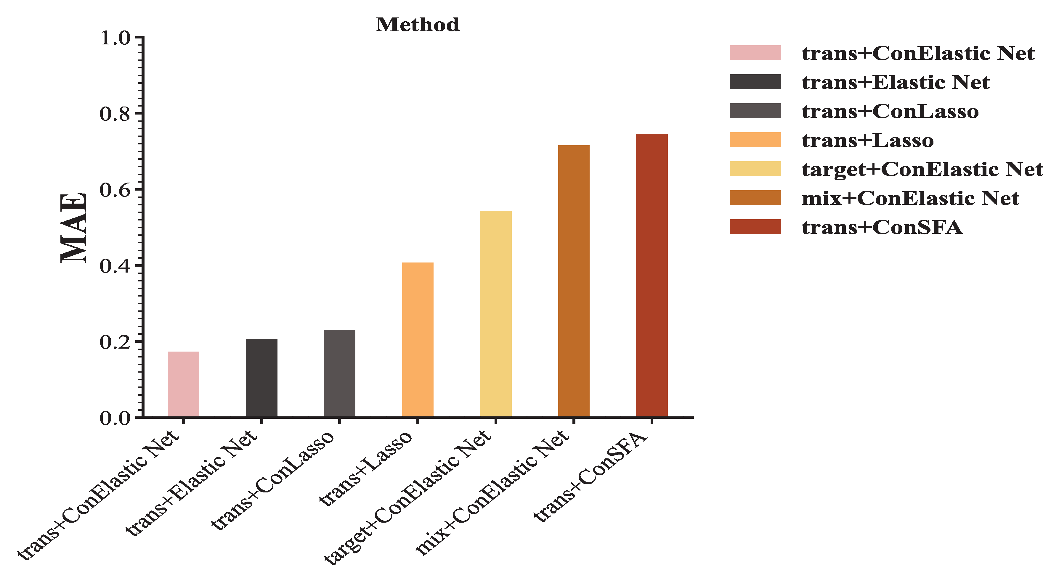
We use the Elastic Net stochastic frontier model with or without linear constraints, the Lasso stochastic frontier model, and the ordinary stochastic frontier model for testing. The results after transfer are shown in Figure 12. The various methods are explained below:

• trans+ConElastic Net: Elastic Net stochastic frontier model with transferable source data and target data under added constraints.
• trans+Elastic Net: Elastic Net stochastic frontier model with transferable source data and target data without adding constraints.
• trans+ConLasso: Lasso stochastic frontier model with transferable source data and target data under added constraints.
• trans+Lasso: Ordinary stochastic frontier model with transferable source data and target data without adding constraints.
• target+ConElastic Net: Elastic Net stochastic frontier model with only target data under linear constraints.
• mix+ConElastic Net: Elastic Net stochastic frontier model with all data under added constraints.
• trans+ConSFA: Ordinary stochastic frontier model with transferable source data and target data under linear constraints.

As shown in Figure 12, trans+conElastic Net achieves the lowest MAE, followed by trans+Elastic Net, which proves the effectiveness of our proposed algorithm. The MAE under constrained conditions is lower than that under unconstrained conditions. Across all methods, this indicates that incorporating prior knowledge during coefficient estimation is beneficial to the estimation results. When all data are used directly for stochastic frontier analysis, a large MAE is observed, further highlighting that the absence of transferable source detection can lead to significant estimation errors.

From

Table 1. Mean ± standard deviation of MAE for each method and paired t-test results compared with the baseline method (trans+ConElastic Net).

Method	MAE	Std	t-Value	p-Value
trans+ConElastic Net	0.1735	±0.1695	–	–
trans+Elastic Net	0.2072	±0.2062	−0.7402	0.4687
trans+ConLasso	0.2307	±0.1870	−0.7204	0.4805
trans+Lasso	0.4073	±0.3453	−3.1678	0.0053 **
target+ConElastic Net	0.5438	±0.5596	−2.3600	0.0298 *
mix+ConElastic Net	0.7156	±0.8451	−2.6351	0.0168 *
trans+ConSFA	0.7446	±0.8776	−2.6911	0.0149 *

Note: * $p<0.05$, ** $p<0.01$ indicate statistically significant differences compared with the baseline method.

, we can see that trans + conElastic Net achieves the lowest standard deviation, and the standard deviation of trans + Elastic Net ranks second, only after trans + ConLasso, indicating that our method is both accurate and stable. We use trans + conElastic Net as the benchmark method for the paired t-test. The results show that, except for the p-values of trans + Elastic Net and trans + ConLasso, the p-values of all other methods reach the significance level $(p<0.05)$, which directly indicates that this method is significantly better than most of the comparison methods in terms of error performance. Combining the results of $MAE$, standard deviation, and the paired t-test, we conclude that our proposed method performs best among the seven candidate methods from multiple perspectives, demonstrating strong practicality and robustness.

5. Discussion

From the above experiments, it can be seen that the transfer learning of the high-dimensional stochastic frontier model via Elastic Net is feasible and effective. Firstly, in the presence of high-dimensional and collinear data, our model outperforms the Lasso stochastic frontier model and ordinary stochastic frontier model. Secondly, adding constraints to the model, that is, incorporating some prior knowledge, can restrict the parameter estimation within a certain range, making the estimation more accurate. Third, transfer learning is used to transfer knowledge from similar source data in the case of limited target data, in order to improve the accuracy of parameter estimation and the performance of prediction. Experiments show that transfer learning is indeed feasible for the high-dimensional stochastic frontier model based on Elastic Net, and greatly improves the performance of the model. Moreover, the effectiveness of both algorithms is demonstrated by simulation experiments and real cases for the scenarios where the transferable source is known and where it is unknown. This study also often observes the phenomenon of negative transfer learning, that is, the negative impact on the final result, which is still very common in transfer learning. How to reduce or avoid the phenomenon of negative transfer learning is a problem for further research in the future. Whether transfer learning can be used for other statistical learning methods will also continue to be studied in the future.

Although the proposed algorithm performs well in numerical simulation and empirical research, it lacks theoretical proof to support its effectiveness. A potential research direction is to provide statistical inference and confidence intervals for the parameters estimated by the proposed method. This will enhance the interpretability and applicability of the algorithm. In addition, extending the existing framework and theoretical analysis to other models is a worthwhile avenue of exploration. Evaluating the applicability of the proposed methods to different models may offer insights into their versatility and potential improvements in various transfer learning scenarios.