A New Class of (α,η,(Q,h),L)-Contractions in Triple Controlled Metric-Type Spaces with Application to Polynomial Sine-Type Equations

Abstract

This paper introduces a novel class of generalized contractions, termed $(\alpha ,\eta ,(Q,h),\mathcal{L})$-contraction mapping, within the context of triple controlled metric-type spaces, extending the framework of fixed point theory in controlled structures. The proposed mapping is defined using $\alpha$-admissible and $\eta$-subadmissible functions, in conjunction with a control pair $(Q,h)$ of upper class of type I, and incorporates Wardowski’s function $\mathcal{L}$-contraction condition. Under suitable hypotheses, we establish both the existence and uniqueness of fixed points for this class of mappings. Several corollaries are derived as special cases of the main result. Moreover, we provide a nontrivial application by analyzing the solvability of a nonlinear equation involving powers of the sine function, thereby illustrating the utility of the developed theory.

1. Introduction

One of the foundational results in fixed point theory is the Banach contraction principle [1], which guarantees the existence and uniqueness of fixed points for self-contractive mappings on complete metric spaces. Since its introduction in 1922, this principle has inspired extensive research, with many generalizations aimed at relaxing the original assumptions and broadening its applicability. One major direction of development has involved generalizing the underlying space. Notably, b-metric spaces, introduced by Bakhtin [2] and refined by Czerwik [3], extend the classical metric structure. This was followed by extended b-metric spaces [4], controlled metric-type spaces [5], controlled b-Branciari metric-type spaces [6], and double controlled metric-type spaces [7,8]. To address increasingly complex systems, recent work has introduced triple controlled metric-type spaces [9,10,11], which employ three control functions to govern the generalized distance. These spaces enable the treatment of nonlinear problems with multiple interdependent constraints, opening new directions for both theory and application. Fixed point theory in such generalized frameworks has found applications across various fields. In ecology, it aids in analyzing equilibrium states in population dynamics and ecosystem models [12]. In computer science, it provides theoretical underpinnings for program semantics, static analysis, and iterative algorithms [13]. In economics, it supports core results in game theory and general equilibrium models [14]. The flexibility of controlled metric spaces makes them particularly valuable in these domains, where classical metric assumptions are often too restrictive.

Fixed point theory on generalized metric-type spaces has seen notable progress with the introduction of several contraction conditions. Among these, Wardowski’s $\mathcal{L}$-contraction [15] and Samet et al.’s $\alpha$-admissible mappings [16] have proven instrumental in relaxing classical assumptions. Recent works (such as [11,17]) have extended these ideas to $(\alpha ,F)$-contractions on various metric frameworks.

To control the iterative behavior in more complex settings, we incorporate a control pair $(Q,h)$ from the upper class of type I, as introduced by Ansari et al. [18,19]. The use of $(Q,h)$ allows for a finer regulation of the contraction dynamics, particularly in triple controlled metric-type spaces. This combination facilitates the establishment of fixed point results under broader and more flexible conditions, with potential applications in nonlinear analysis and applied mathematics.

In this work, we introduce a novel contraction mapping, denoted by ($\alpha ,\eta ,(Q,h),\mathcal{F}$)-contractions, within the framework of triple controlled metric-type spaces. These mappings incorporate the following:

• $\alpha$-admissible and $\eta$-subadmissible control functions.
• a control pair $(Q,h)$ from the upper class of type I.
• a function-based contraction condition of Wardowski type via $\mathcal{L}$-functions.

We establish both the existence and uniqueness of fixed points for these mappings and derive several corollaries as special cases of our main result. In addition, we present an example of our main result.

To demonstrate the applicability of the proposed theory, we analyze a nonlinear equation involving powers of the $sin\left(\xi \right)$ function,

$${sin}^r\left(\xi \right)-(r^4-1){sin}^{r+1}\left(\xi \right)-r^{4}sin\left(\xi \right)+1=0,$$

by first establishing the existence and uniqueness of a real root of an mth-degree polynomial in x. Then, as an application, we apply it to the $x=sin\left(\xi \right)$ function, thereby illustrating how our framework effectively handles analytical problems involving nonlinear trigonometric expressions.

2. Preliminaries

In 2000, Branciari [20] introduced the notion of rectangular metric spaces, also known as generalized metric spaces.

Definition 1.

The mapping $d:{\mathcal{X}}^2\to [0,\infty )$, with $\mathcal{X}\ne \varnothing$, is defined as follows:

1. 

$d({\chi }_1,{\chi }_2)=0⟺{\chi }_1={\chi }_2$, for all ${\chi }_1,{\chi }_2\in \mathcal{X}$;

2. 

$d({\chi }_1,{\chi }_2)=d({\chi }_2,{\chi }_1),$ the symmetry property for all ${\chi }_1,{\chi }_2\in \mathcal{X}$;

3. 

$d({\chi }_1,{\chi }_2)\le d({\chi }_1,{\chi }_3)+d({\chi }_3,{\chi }_4)+d({\chi }_4,{\chi }_2).$

The pair $(\mathcal{X},d)$ is called a rectangular metric space.

Rectangular metric spaces have attracted considerable interest, as their topological structure is generally incompatible with that of ordinary metric spaces. This fundamental distinction has motivated numerous authors to further explore and develop the theory of such spaces [21]. The concept was subsequently extended to rectangular b-metric spaces [22,23]. More recently, in 2020, the controlled b-Branciari metric-type space was introduced [6], providing an even more flexible framework.

Definition 2.

Let $\mathcal{X}\ne \varnothing$, and consider a real number $s\ge 1$. The mapping $d:{\mathcal{X}}^2\to [0,\infty )$ is defined as follows:

1. 

$d({\chi }_1,{\chi }_2)=0⟺{\chi }_1={\chi }_2$, for all ${\chi }_1,{\chi }_2\in \mathcal{X}$;

2. 

$d({\chi }_1,{\chi }_2)=d({\chi }_2,{\chi }_1),$ the symmetry property for all ${\chi }_1,{\chi }_2\in \mathcal{X}$;

3. 

$d({\chi }_1,{\chi }_2)\le s[d({\chi }_1,{\chi }_3)+d({\chi }_3,{\chi }_4)+d({\chi }_4,{\chi }_2)],$

for all ${\chi }_1,{\chi }_2\in \mathcal{X}$ and all distinct points ${\chi }_3,{\chi }_4\in \mathcal{X}$, each different from ${\chi }_1,{\chi }_2$. The structure $(\mathcal{X},d)$ is called a rectangular b-metric space.

Definition 3.

Let $\mathcal{X}\ne \varnothing$ and consider $\beta :\mathcal{X}\times \mathcal{X}\to [1,\infty )$. A function $d:\mathcal{X}\times \mathcal{X}\to [0,\infty )$ is referred to as a controlled b-Branciari type metric if it fulfills the following conditions:

1. 

$d({\chi }_1,{\chi }_2)=0⟺{\chi }_1={\chi }_2$, for all ${\chi }_1,{\chi }_2\in X$;

2. 

$d({\chi }_1,{\chi }_2)=d({\chi }_2,{\chi }_1),$ symmetry condition for all ${\chi }_1,{\chi }_2\in X$;

3. 

$d({\chi }_1,{\chi }_2)\le \beta ({\chi }_1,{\chi }_3)d({\chi }_1,{\chi }_3)+\beta ({\chi }_3,{\chi }_4)d({\chi }_3,{\chi }_4)+\beta ({\chi }_4,{\chi }_2)d({\chi }_4,{\chi }_2).$

For every pair ${\chi }_1,{\chi }_2$ that belongs to $\mathcal{X}$, and for all distinct elements ${\chi }_3,{\chi }_4\in \mathcal{X}$, each different from ${\chi }_1,{\chi }_2$. The structure $(\mathcal{X},d)$ is termed a controlled b-Branciari metric-type space.

The triple controlled metric-type space was introduced as an extension to the controlled b-Branciari metric-type space. For more information, consult [9,10,11].

Definition 4.

([9]). Consider $\mathcal{X}\ne \varnothing$, let $\beta ,\mu ,\gamma :\mathcal{X}\times \mathcal{X}\to [1,\infty )$ be functions. A mapping $\varpi :{\mathcal{X}}^2\to [0,\infty )$ is termed as a triple controlled metric type if it satisfies the following:

(q1)

$\varpi ({\chi }_1,{\chi }_2)=0$ if and only if ${\chi }_1={\chi }_2,$ for every ${\chi }_1,{\chi }_2\in \mathcal{X}$;

(q2)

$\varpi ({\chi }_1,{\chi }_2)=\varpi ({\chi }_2,{\chi }_1),$ for every ${\chi }_1,{\chi }_2\in \mathcal{X}$;

(q3)

$\varpi ({\chi }_1,{\chi }_2)\le \beta ({\chi }_1,{\chi }_3)\varpi ({\chi }_1,{\chi }_3)+\mu ({\chi }_3,{\chi }_4)\varpi ({\chi }_3,{\chi }_4)+\gamma ({\chi }_4,{\chi }_2)\varpi ({\chi }_4,{\chi }_2)$.

For every ${\chi }_1,{\chi }_2\in \mathcal{X}$ and for every distinct elements ${\chi }_3,{\chi }_4\in \mathcal{X},$ each different from ${\chi }_1$ and ${\chi }_2$. The structure $(\mathcal{X},\varpi )$ is termed a triple controlled metric-type space (it is abbreviated as $\mathcal{TC}MTS$).

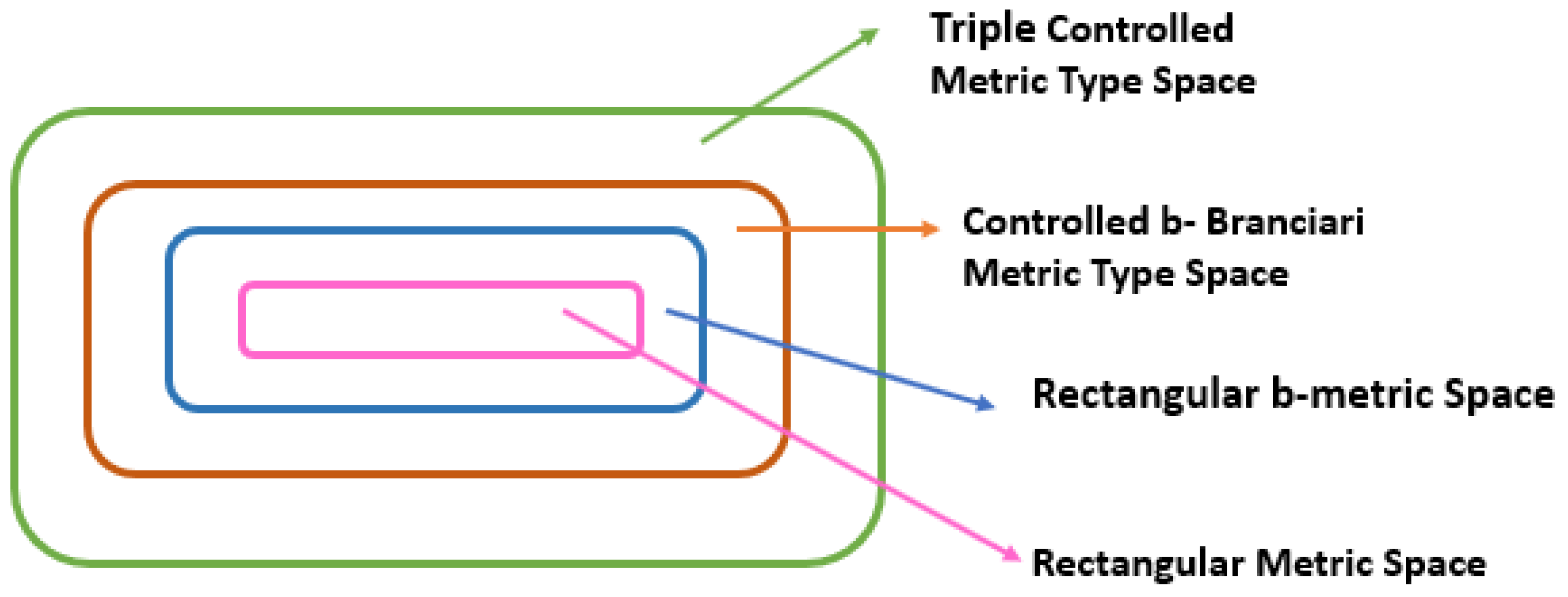
Remark 1.

The relationship between these various rectangular metric-type spaces can be observed as follows: by taking $s=1$, one can see that every rectangular metric space is a rectangular b-metric-type space. Also, by taking the function $\beta =s$, we observe that every rectangular b-metric space is a controlled b-Branciari metric-type space. Moreover, by taking $\beta =\mu =\gamma$, we conclude that every controlled b-Branciari metric-type space is a triple controlled metric-type space. The converse does not hold in any of these cases. Figure 1 below illustrates the relationship between various metric spaces.

The triple controlled metric-type space, $\mathcal{TC}MTS$, is a generalization of controlled b-Branciari metric-type space, as illustrated in the example below (c.f. [9]).

Example 1.

Let $A=\mathcal{X}\cup \mathcal{Y}$, where $\mathcal{X}=\{{\displaystyle \frac{1}{n}}:n\in N\}$ and $\mathcal{Y}$ is the set of all positive integers. Define the mapping $\varpi :A\times A\to [0,\infty )$ by

$$\varpi ({\chi }_1,{\chi }_2)=\left\{\begin{array}{cc}0\hfill & iff{\chi }_1={\chi }_2,\hfill \\ {\chi }_1+10\hfill & if{\chi }_1\in \mathcal{X},{\chi }_2\in \{6,9\},\mathit{or}{\chi }_1\in \{6,9\},{\chi }_2\in \mathcal{X},\hfill \\ 2\hfill & \mathit{otherwise}.\hfill \end{array}\right.$$

The control functions $\beta ,\mu ,\gamma :A\times A\to [1,\infty )$ are defined as

$$\beta ({\chi }_1,{\chi }_2)=\left\{\begin{array}{cc}{\displaystyle \frac{1}{{\chi }_1}}\hfill & \mathit{if}{\chi }_1\in \mathcal{X},{\chi }_2\in \mathcal{Y},\hfill \\ 1\hfill & \mathit{otherwise}.\hfill \end{array}\right.$$

$$\mu ({\chi }_1,{\chi }_2)=\left\{\begin{array}{cc}{\chi }_1+{\chi }_2\hfill & \mathit{if}{\chi }_1\in \mathcal{X},{\chi }_2\in \mathcal{Y},\hfill \\ 2\hfill & \mathit{otherwise},\hfill \end{array}\right.$$

and

$$\gamma ({\chi }_1,{\chi }_2)=\left\{\begin{array}{cc}{\chi }_1+1\hfill & \mathit{if}\mathit{both}{\chi }_1,{\chi }_2\in \mathcal{X},\mathrm{or}{\chi }_1,{\chi }_2\in \mathcal{Y},\hfill \\ {\displaystyle \frac{3}{2}}\hfill & \mathit{otherwise}.\hfill \end{array}\right.$$

One can easily show that ϖ is a $\mathcal{TC}MTS$. Note

$$\varpi ({\displaystyle \frac{1}{3}},9)={\displaystyle \frac{31}{3}}>\beta ({\displaystyle \frac{1}{3}},4)\varpi ({\displaystyle \frac{1}{3}},4)+\beta (4,1)\varpi (4,1)+\beta (1,9)\varpi (1,9)=10.$$

Thus, the $\mathcal{TC}MTS$ is not a controlled b-Branciari metric-type space.

The notions of convergence, Cauchy sequences, completeness, and open balls within the framework of $\mathcal{TC}MTS$ are presented in the following discussion.

Definition 5.

Consider the $\mathcal{TC}MTS$ structure $(\mathcal{X},\varpi )$, and assume $\left\{{\chi }_n\right\}$ is any sequence in the space $\mathcal{X}$.

(1) 

The operator $T:\mathcal{X}\to \mathcal{X}$ is termed to be continuous at point ${\chi }_0\in \mathcal{X},$ if for every $\epsilon >0$, there exists $t>0$ so that $T\left(B({\chi }_0,t)\right)\subseteq B(T{\chi }_0,\epsilon )$.

(2) 

The open ball $B(\chi ,\epsilon )$ is described as

$$B(\chi ,\epsilon )=\{{\chi }_1\in \mathcal{X},\varpi (\chi ,{\chi }_1)<\epsilon \},$$

for some $\epsilon >0$ and $\chi \in \mathcal{X}$.

(3) 

A sequence $\left\{{\chi }_n\right\}$ in $\mathcal{X}$ is termed to converge to some ${\chi }_0$ in $\mathcal{X},$ if for every $\epsilon >0$, you can find some $N\in \mathbb{N},$ so that $\varpi ({\chi }_n,{\chi }_0)<\epsilon$ for every $n\ge N.$ In this case, we write ${lim}_{n\to \infty }{\chi }_n={\chi }_0.$

(4) 

The sequence $\left\{{\chi }_n\right\}$ is said to be a Cauchy sequence, if for every $\epsilon >0$, there exists some $N\in \mathbb{N}$ such that $\varpi ({\chi }_m,{\chi }_n)<\epsilon$ for every $m,n\ge N.$

(5) 

The space $(\mathcal{X},\varpi )$ is said to be a complete space if every Cauchy sequence in $\mathcal{X}$ is convergent.

Remark 2.

In light of the disparities between the rectangular b-metric space topology and the conventional metric space topology, an illustrative example, initially constructed in [24] and further discussed in subsequent studies [23,25], demonstrates a fundamental distinction. Unlike traditional metric spaces, where each convergent sequence has a unique limit, in b-metric spaces, sequences may converge to multiple limits. This property highlights a significant deviation from the standard sequence convergence’s behavior within metric spaces.

Example 2.

Let $\mathcal{X}=\{0,2\}$, $\mathcal{Y}=\{{\displaystyle \frac{1}{n}}:n\in \mathbb{N}\}$ and consider the set $W=\mathcal{X}\cup \mathcal{Y}$. The mapping $\delta :W\times W\to [0,\infty )$ is defined as

$$\delta ({\chi }_1,{\chi }_2)=\left\{\begin{array}{cc}0,\hfill & {\chi }_1={\chi }_2,\hfill \\ 1\hfill & {\chi }_2\ne {\chi }_1,\mathrm{and}\{{\chi }_1,{\chi }_2\}\subset \mathcal{X}\mathrm{or}\{{\chi }_1,{\chi }_2\}\subset \mathcal{Y},\hfill \\ {\chi }_2,\hfill & {\chi }_1\in \mathcal{X},{\chi }_2\in \mathcal{Y},\hfill \\ {\chi }_1,\hfill & {\chi }_1\in \mathcal{X},{\chi }_2\in \mathcal{Y}.\hfill \end{array}\right.$$

Consider $K({\chi }_1,{\chi }_2)=\delta {({\chi }_1,{\chi }_2)}^2$, and $s=3$, then one can see that $(W,K)$ is a rectangular b-metric space. Note that the sequence $\left\{{\displaystyle \frac{1}{n}}\right\}$ converges to two elements 0 and 2. For more illustrations, refer to [23,24].

The next lemma, adapted from [26] and further explored in [23,25], illustrates the condition that guarantees the unique convergence of a sequence in b-metric spaces.

Lemma 1. 

Let $\left\{{\chi }_n\right\}$ be a Cauchy sequence in a rectangular b-metric space $(\mathcal{X},\varpi )$ with the property that ${\chi }_m\ne {\chi }_n$ for all $m\ne n$. Under these conditions, the sequence $\left\{{\chi }_n\right\}$ admits at most one limit point.

Definition 6

([18,19]). A map $h:R^{+}\times R^{+}\to R$ belongs to the subclass of type I if it fulfills the following condition: for all $a,b\in R^{+},$ whenever $a\ge 1$, it holds that $h(1,b)\le h(a,b).$

Example 3

([18,19]). Each function h is of a subclass of type I:

(1) 

let $h(a,b)={(b+l)}^a,$ with $l>1$.

(2) 

let $h(a,b)={(a+l)}^b$, with $l>0$.

(3) 

let $h(a,b)=a^n{b}^k,$ such that $k>0,n\in \mathbb{N}\cup \left\{0\right\}$.

Definition 7

([18,19]). The pair $(Q,h)$ is called an upper class of type I, if h is of a subclass of type I, and $Q:R^{+}\times R^{+}\to R$ is a function fulfilling the following conditions:

1. 

$0\le r\le 1$ implies $Q(r,t)\le Q(1,t),$

2. 

$h(1,b)\le Q(r,t)$ implies $b\le rt,\mathrm{for}\mathrm{all}b,r,t\in R^{+}.$

Example 4

([18,19]). Examples of the pair $(Q,h)$:

(1) 

Let $h(a,b)={(b+l)}^a,$ with $l>1$ and,$Q(r,t)=rt+l.$

(2) 

Let $h(a,b)={(a+l)}^b,l>0,$ and $Q(s,t)={(1+l)}^{st}$.

(3) 

Let $h(a,b)=a^n{b}^k,$ and $Q(s,t)=s^m{t}^k,$ and $k>0$.

(4) 

Let $h(a,b)={\displaystyle \frac{ma+n}{m+n}}b,$ with $m,n\in N,$ and $Q(s,t)=st$.

The notion of $\alpha$-admissible mappings was proposed by Samet et al. [16], while the notion $\eta$-subadmissible mapping can be found in [27].

Definition 8.

Consider the mapping $T:\mathcal{X}⟶\mathcal{X}$ and let $\alpha ,\eta :\mathcal{X}\times \mathcal{X}\to [0,\infty )$ be functions. Then,

(1) 

T is referred to as $\alpha$-admissible mapping, if for all ${\chi }_1,{\chi }_2\in \mathcal{X}$, we have

$$\alpha ({\chi }_1,{\chi }_2)\ge 1⟹\alpha (T{\chi }_1,T{\chi }_2)\ge 1.$$

(2) 

T is referred to as η-subadmissible mapping, if for all ${\chi }_1,{\chi }_2\in \mathcal{X}$, we have

$$\eta ({\chi }_1,{\chi }_2)\le 1⟹\eta (T{\chi }_1,T{\chi }_2)\le 1.$$

Example 5.

Consider $\mathcal{A}=[0,+\infty )$, and let $T:\mathcal{A}⟶\mathcal{A}$ and $\alpha :{\mathcal{A}}^2\to [0,\infty )$ be defined as $T\left(\chi \right)=7\chi$, and for all ${\chi }_1,{\chi }_2\in \mathcal{A}$,

$$\alpha ({\chi }_1,{\chi }_2)=\left\{\begin{array}{cc}{e}^{{\displaystyle \frac{{\chi }_2}{{\chi }_1}}},\hfill & \mathit{if}{\chi }_1\ge {\chi }_2,{\chi }_1\ne 0.\hfill \\ 0\hfill & \mathit{if}{\chi }_1<{\chi }_2.\hfill \end{array}\right.$$

Then, T is termed as $\alpha$-admissible mapping

Example 6.

Let $\mathcal{X}=[0,+\infty )$, the mapping $T:\mathcal{X}\to \mathcal{X}$ is defined as;

$$T\left(\chi \right)=\left\{\begin{array}{cc}{\displaystyle \frac{\chi }{4}}\hfill & \mathit{if}\chi \in [0,1],\hfill \\ 2\chi -{\displaystyle \frac{7}{4}}\hfill & \mathit{if}\chi >1.\hfill \end{array}\right.$$

Let $\alpha ,\eta :{\mathcal{X}}^2\to (-\infty ,+\infty )$ be defined by

$$\alpha ({\chi }_1,{\chi }_2)=\left\{\begin{array}{cc}1\hfill & \mathit{if}{\chi }_1,{\chi }_2\in [0,1],\hfill \\ 0\hfill & \mathit{otherwise},\hfill \end{array}\right.$$

and

$$\eta ({\chi }_1,{\chi }_2)=\left\{\begin{array}{cc}1\hfill & \mathit{if}{\chi }_1,{\chi }_2\in [0,1],\hfill \\ 2\hfill & \mathit{otherwise}.\hfill \end{array}\right.$$

Then, T is α-admissible and η-subadmissible mapping, since if $\alpha ({\chi }_1,{\chi }_2)\ge 1,$ means ${\chi }_1,{\chi }_2\in [0,1]$, consequently, $\alpha (T{\chi }_1,T{\chi }_2)=\alpha ({\displaystyle \frac{{\chi }_1}{4}},{\displaystyle \frac{{\chi }_2}{4}})\ge 1.$ Moreover, T is η-subadmissible, since if $\eta ({\chi }_1,{\chi }_2)\le 1$, means ${\chi }_1,{\chi }_2\in [0,1]$, hence $\eta (T{\chi }_1,T{\chi }_2)=\eta ({\displaystyle \frac{{\chi }_1}{4}},{\displaystyle \frac{{\chi }_2}{4}})\le 1$.

Wardowski [15] introduced the $\mathcal{L}$-contraction, later extended to various generalized metric spaces [28,29].

Definition 9.

Define $\mathcal{L}$ as the collection of all functions $L:(0,\infty )\to (-\infty ,\infty )$ that meet the following conditions:

(L1)

L is a strictly increasing.

(L2)

For any sequence $\left\{s_n\right\}$ of positive real numbers, the equivalence;

$$\underset{n\to \infty }{lim}{s}_n=0\iff \underset{n\to \infty }{lim}L\left(s_n\right)=-\infty ,$$

holds true.

(L3)

There exists a constant $r\in (0,1)\ni {lim}_{s\to 0^{+}}{s}^{r}L\left(s\right)=0$.

Example 7.

Let $F\left(t\right)={\displaystyle \frac{-1}{\sqrt{t}}}$, and $G\left(t\right)=ln\left(t\right)$, for $t>0$. It is evident that both F(t) and G(t) fulfill the conditions $\left(L1\right),\left(L2\right)$, and $\left(L3\right)$. Therefore, they are member of the class $\mathcal{L}$. For additional information, refer to [15].

Definition 10.

Let $(\mathcal{X},\varpi )$ be a $\mathcal{TC}MTS$. A self-mapping $T:\mathcal{X}\to \mathcal{X}$ is said to be $\mathcal{L}$-contraction if there exists a function $L\in$$\mathcal{L}$ and a constant $\tau >0$ such that the following implication holds:

$$\varpi (T{\chi }_1,T{\chi }_2)>0\Rightarrow \tau +L\left(\varpi (T{\chi }_1,T{\chi }_2)\right)\le L\left(\varpi ({\chi }_1,{\chi }_2)\right),for{\chi }_1,{\chi }_2\in \mathcal{X}.$$

(1)

Next, we present our novel $(\alpha ,\eta ,(Q,h),\mathcal{L})$—contraction mapping on a $\mathcal{TC}MTS$$(\mathcal{X},\varpi )$.

Definition 11.

Let $(\mathcal{X},\varpi )$ be a $\mathcal{TC}MTS$, where $\mathcal{X}\ne \varnothing$. A mapping $T:\mathcal{X}\to \mathcal{X}$ is considered to be an $(\alpha ,\eta ,(Q,h),\mathcal{L})$—contraction, if the following inequality is satisfied:

$$h\left(\alpha (x,y),\tau +L\left(\varpi \right(Tx,Ty)\right)\le Q\left(\eta (x,y),L\left(\varpi \right(x,y\left)\right)\right),$$

(2)

for every $x,y\in \mathcal{X}$, such that $\varpi (Tx,Ty)>0$, and $\tau >0$. The pair $(Q,h)$ is an upper class of type I, here α and η as in Definition 8.

Example 8.

Let $(\mathcal{X},\varpi )$ be a $\mathcal{TC}MTS$, and let the mapping $T:\mathcal{X}\to \mathcal{X}$ be an $(\alpha ,\eta ,(Q,h),\mathcal{L})$-contraction mapping. By taking $h(x,y)=x^n{y}^k$ and $Q(s,t)=s^m{t}^k,$ where $m,n\in \mathbb{N}\cup \left\{0\right\},$ and $k>0$, and $L\left(s\right)=ln\left(s\right)$, thus Equation (2) simplifies to

$$\alpha {(x,y)}^n{(\tau +ln\left(\varpi (Tx,Ty)\right))}^k\le \eta {(x,y)}^{m}ln{\left(\varpi (x,y)\right)}^k.$$

(3)

3. Main Results

The primary fixed-point result based on our novel $(\alpha ,\eta ,(Q,h),\mathcal{L})$-contraction mapping (defined on $\mathcal{TC}MTS$, $(\mathcal{X},\varpi )$) framework is presented below.

Theorem 1.

Let $(\mathcal{X},\varpi )$ be a complete $\mathcal{TC}MTS$, and let $T:\mathcal{X}\to \mathcal{X}$ be an $(\alpha ,\eta ,(Q,h),\mathcal{L})$-contraction mapping, as in Definition 11, satisfying the following conditions:

(T1) 

T is both α-admissible and η-subadmissible.

(T2) 

Some ${\chi }_0\in \mathcal{X}$ can be found, so that $\alpha ({\chi }_0,T{\chi }_0)\ge 1$ and $\eta ({\chi }_0,T{\chi }_0)\le 1$.

(T3) 

For ${\chi }_0\in \mathcal{X}$, we define the sequence $\left\{{\chi }_n\right\}$ by ${\chi }_n=T^n{\chi }_0$, for $n\in \mathbb{N}$. Assume the following conditions hold:

$$\underset{m\ge 1}{sup}\underset{i\to \infty }{lim}{\displaystyle \frac{\beta ({\chi }_{2i+2},{\chi }_{2i+3})}{\beta ({\chi }_{2i},{\chi }_{2i+1})}}\gamma ({\chi }_{2i+2},{\chi }_m)<1,$$

(4)

and

$$\underset{m\ge 1}{sup}\underset{i\to \infty }{lim}{\displaystyle \frac{\mu ({\chi }_{2i+3},{\chi }_{2i+4})}{\mu ({\chi }_{2i+1},{\chi }_{2i+2})}}\gamma ({\chi }_{2i+2},{\chi }_m)<1.$$

(5)

Furthermore, for each $\tilde{\chi }\in \mathcal{X}$, the following limits exists and are finite;

$$\underset{n\to \infty }{lim}\beta (\tilde{\chi },{\chi }_n),\underset{n\to \infty }{lim}\mu ({\chi }_n,\tilde{\chi })\mathrm{and}\underset{n\to \infty }{lim}\gamma ({\chi }_n,\tilde{\chi }).$$

(6)

Then T admits a fixed point in $\mathcal{X}$. Moreover, if T has two fixed points ${\tilde{\chi }}_1,{\tilde{\chi }}_2\in \mathcal{X}$ satisfying $\alpha ({\tilde{\chi }}_1,{\tilde{\chi }}_2)\ge 1$ and $\eta ({\tilde{\chi }}_1,{\tilde{\chi }}_2)\le 1$, then T possess a unique fixed point in $\mathcal{X}.$

Proof. 

We start by selecting ${\chi }_0$ as in condition (T2), hence $\alpha ({\chi }_0,T{\chi }_0)\ge 1$, and $\eta ({\chi }_0,T{\chi }_0)\le 1$. The general term of the sequence $\left\{{\chi }_n\right\}$ is defined by setting $T{\chi }_0={\chi }_1,T^2{\chi }_0=T{\chi }_1={\chi }_2$. For any $n\in \mathbb{N}$, we have

$$T^n{\chi }_0=T^{n-1}{\chi }_1=\cdots =T{\chi }_{n-1}={\chi }_n.$$

By utilizing the pair $(Q,h)$:

$$\begin{array}{cc}\hfill h\left(1,\tau +L\left(\varpi ({\chi }_n,{\chi }_{n+1})\right)\right)& =h\left(1,\tau +L\left(\varpi (T{\chi }_{n-1},T{\chi }_n)\right)\right).\hfill \\ \hfill & \le h\left(\alpha ({\chi }_{n-1},{\chi }_n),\tau +L\left(\varpi (T{\chi }_{n-1},T{\chi }_n)\right)\right).\hfill \\ \hfill & \le Q\left(\eta ({\chi }_{n-1},{\chi }_n),L\left(\varpi ({\chi }_{n-1},{\chi }_n)\right)\right).\hfill \\ \hfill & \le Q\left(1,L\left(\varpi ({\chi }_{n-1},{\chi }_n)\right)\right).\hfill \end{array}$$

Which gives

$$\tau +L\left(\varpi ({\chi }_n,{\chi }_{n+1})\right)\le L\left(\varpi ({\chi }_{n-1},{\chi }_n)\right).$$

After continuing the process a few times,

$$\begin{array}{ccc}\hfill L\left(\varpi ({\chi }_n,{\chi }_{n+1})\right)& \le & L\left(\varpi ({\chi }_{n-1},{\chi }_n)\right)-\tau .\hfill \\ \hfill & \le & L\left(\varpi ({\chi }_{n-2},{\chi }_{n-1})\right)-2\tau .\hfill \\ \hfill & \le & \cdots \le L\left(\varpi ({\chi }_0,{\chi }_1)\right)-n\tau .\hfill \end{array}$$

(7)

Taking the limit $n\to +\infty$ in (7), and utilizing $\tau >0$,

$$\underset{n\to +\infty }{lim}L\left(\varpi ({\chi }_n,{\chi }_{n+1})\right)=-\infty .$$

(8)

As $L\in$$\mathcal{L}$, by (L2), it implies that ${lim}_{n\to +\infty }\varpi ({\chi }_n,{\chi }_{n+1})=0$. By condition (L3), we can find some $k\in (0,1),$ such that

$$\underset{n\to +\infty }{lim}{\left(\varpi ({\chi }_n,{\chi }_{n+1})\right)}^{k}L\left(\varpi ({\chi }_n,{\chi }_{n+1})\right)=0.$$

(9)

Utilizing (7), we get

$$L\left(\varpi ({\chi }_n,{\chi }_{n+1})\right)-L\left(\varpi ({\chi }_0,{\chi }_1)\right)\le -n\tau .$$

Which gives

$${\left(\varpi ({\chi }_n,{\chi }_{n+1})\right)}^{k}L\left(\varpi ({\chi }_n,{\chi }_{n+1})\right)-{\left(\varpi ({\chi }_n,{\chi }_{n+1})\right)}^{k}L\left(\varpi ({\chi }_0,{\chi }_1)\right)$$

$$\le -n\tau {\left(\varpi ({\chi }_n,{\chi }_{n+1})\right)}^k\le 0.$$

(10)

Letting n tends to infinity in Equation (10), we obtain

$$\underset{n\to +\infty }{lim}n({\left(\varpi ({\chi }_n,{\chi }_{n+1})\right)}^k=0.$$

(11)

Therefore, ${lim}_{n\to +\infty }{n}^{1/k}\left(\varpi ({\chi }_n,{\chi }_{n+1})\right)=0$; thus, there is some $n_0\in \mathbb{N}$ so that

$$\varpi ({\chi }_n,{\chi }_{n+1})\le {\displaystyle \frac{1}{n^{1/k}}},foralln\ge n_0.$$

(12)

Step A: Establishing the convergence of the sequence $\left\{{\chi }_n\right\}$.

We start by showing $\left\{{\chi }_n\right\}$ is Cauchy sequence in two steps; thus, for all, $m,n\in \mathbb{N}$:

Step 1. Assume that $p=2m+1$ is an odd integer, where $m\ge 1$. By applying triangular inequality in the context of the $\mathcal{TC}MTS$, we derive:

$$\begin{array}{cc}\hfill \varpi ({\chi }_n,{\chi }_{n+2m+1})& \le \beta ({\chi }_n,{\chi }_{n+1})\varpi ({\chi }_n,{\chi }_{n+1})+\mu ({\chi }_{n+1},{\chi }_{n+2})\varpi ({\chi }_{n+1},{\chi }_{n+2})\hfill \\ \hfill & +\gamma ({\chi }_{n+2},{\chi }_{n+2m+1})\varpi ({\chi }_{n+2},{\chi }_{n+2m+1}).\hfill \\ \hfill & \le \beta ({\chi }_n,{\chi }_{n+1})\varpi ({\chi }_n,{\chi }_{n+1})+\mu ({\chi }_{n+1},{\chi }_{n+2})\varpi ({\chi }_{n+1},{\chi }_{n+2})\hfill \\ \hfill & +\gamma ({\chi }_{n+2},{\chi }_m)[\beta ({\chi }_{n+2},{\chi }_{n+3})\varpi ({\chi }_{n+2},{\chi }_{n+3})+\mu ({\chi }_{n+3},{\chi }_{n+4})\varpi ({\chi }_{n+3},{\chi }_{n+4})\hfill \\ \hfill & +\gamma ({\chi }_{n+4},{\chi }_{n+2m+1})\varpi ({\chi }_{n+4},{\chi }_{n+2m+1})].\hfill \\ \hfill ⋮\end{array}$$

$$\begin{array}{cc}\hfill \varpi ({\chi }_n,{\chi }_{n+2m+1})& \le \beta ({\chi }_n,{\chi }_{n+1})\varpi ({\chi }_n,{\chi }_{n+1})+\mu ({\chi }_{n+1},{\chi }_{n+2})\varpi ({\chi }_{n+1},{\chi }_{n+2})\hfill \\ \hfill & +\sum _{i={\displaystyle \frac{n}{2}}+1}^{{\displaystyle \frac{n+2m-2}{2}}}[\beta ({\chi }_{2i},{\chi }_{2i+1})\varpi ({\chi }_{2i},{\chi }_{2i+1})+\mu ({\chi }_{2i+1},{\chi }_{2i+2})\varpi ({\chi }_{2i+1},{\chi }_{2i+2})]\hfill \\ \hfill & \left(\prod _{j={\displaystyle \frac{n}{2}}+1}^i\gamma ({\chi }_{2j},{\chi }_{n+2m+1})\right)+\prod _{i={\displaystyle \frac{n}{2}}+1}^{{\displaystyle \frac{n+2m}{2}}}\gamma ({\chi }_{2i},{\chi }_{n+2m+1})\varpi ({\chi }_{n+2m},{\chi }_{n+2m+1}).\hfill \\ \hfill & \le \beta ({\chi }_n,{\chi }_{n+1})\varpi ({\chi }_n,{\chi }_{n+1})+\mu ({\chi }_{n+1},{\chi }_{n+2})\varpi ({\chi }_{n+1},{\chi }_{n+2})\hfill \\ \hfill & +\sum _{i={\displaystyle \frac{n}{2}}+1}^{{\displaystyle \frac{n+2m-2}{2}}}\beta ({\chi }_{2i},{\chi }_{2i+1})\varpi ({\chi }_{2i},{\chi }_{2i+1})\left(\prod _{j={\displaystyle \frac{n}{2}}+1}^i\gamma ({\chi }_{2j},{\chi }_{n+2m+1})\right)\hfill \\ \hfill & +\prod _{i={\displaystyle \frac{n}{2}}+1}^{{\displaystyle \frac{n+2m}{2}}}\gamma ({\chi }_{2i},{\chi }_{n+2m+1})\varpi ({\chi }_{n+2m},{\chi }_{n+2m+1})\hfill \\ \hfill & +\sum _{i={\displaystyle \frac{n}{2}}+1}^{{\displaystyle \frac{n+2m-2}{2}}}\mu ({\chi }_{2i+1},{\chi }_{2i+2})\varpi ({\chi }_{2i+1},{\chi }_{2i+2})\left(\prod _{j={\displaystyle \frac{n}{2}}+1}^i\gamma ({\chi }_{2j},{\chi }_{n+2m+1})\right).\hfill \end{array}$$

The last inequality can be written as

$$\begin{array}{cc}\hfill \varpi ({\chi }_n,{\chi }_{n+2m+1})& \le \beta ({\chi }_n,{\chi }_{n+1})\varpi ({\chi }_n,{\chi }_{n+1})+\mu ({\chi }_{n+1},{\chi }_{n+2})\varpi ({\chi }_{n+1},{\chi }_{n+2})\hfill \\ \hfill & +\sum _{i={\displaystyle \frac{n}{2}}+1}^{{\displaystyle \frac{n+2m}{2}}}\beta ({\chi }_{2i},{\chi }_{2i+1})\varpi ({\chi }_{2i},{\chi }_{2i+1})\left(\prod _{j={\displaystyle \frac{n}{2}}+1}^i\gamma ({\chi }_{2j},{\chi }_{n+2m+1})\right)\hfill \\ \hfill & +\sum _{i={\displaystyle \frac{n}{2}}+1}^{{\displaystyle \frac{n+2m-2}{2}}}\mu ({\chi }_{2i+1},{\chi }_{2i+2})\varpi ({\chi }_{2i+1},{\chi }_{2i+2})\left(\prod _{j={\displaystyle \frac{n}{2}}+1}^i\gamma ({\chi }_{2j},{\chi }_{n+2m+1})\right).\hfill \end{array}$$

By substituting Equation (12) into the preceding inequality, we conclude that

$$\varpi ({\chi }_{2i},{\chi }_{2i+1})\le {\displaystyle \frac{1}{{\left(2i\right)}^{1/k}}},$$

which leads to

$$\begin{array}{cc}\hfill \varpi ({\chi }_n,{\chi }_{n+2m+1})& \le \beta ({\chi }_n,{\chi }_{n+1}){\displaystyle \frac{1}{{\left(n\right)}^{1/k}}}+\mu ({\chi }_{n+1},{\chi }_{n+2}){\displaystyle \frac{1}{{(n+1)}^{1/k}}}\hfill \\ \hfill & +\sum _{i={\displaystyle \frac{n}{2}}+1}^{{\displaystyle \frac{n+2m}{2}}}\beta ({\chi }_{2i},{\chi }_{2i+1})\left(\prod _{j={\displaystyle \frac{n}{2}}+1}^i\gamma ({\chi }_{2j},{\chi }_{n+2m+1})\right){\displaystyle \frac{1}{{\left(2i\right)}^{1/k}}}\hfill \\ \hfill & +\sum _{i={\displaystyle \frac{n}{2}}+1}^{{\displaystyle \frac{n+2m-2}{2}}}\mu ({\chi }_{2i+1},{\chi }_{2i+2})\left(\prod _{j={\displaystyle \frac{n}{2}}+1}^i\gamma ({\chi }_{2j},{\chi }_{n+2m+1})\right){\displaystyle \frac{1}{{(2i+1)}^{1/k}}}.\hfill \end{array}$$

We express it as

$$\begin{array}{cc}\hfill \varpi ({\chi }_n,{\chi }_{n+2m+1})& \le \beta ({\chi }_n,{\chi }_{n+1}){\displaystyle \frac{1}{{\left(n\right)}^{1/k}}}+\mu ({\chi }_{n+1},{\chi }_{n+2}){\displaystyle \frac{1}{{(n+1)}^{1/k}}}\hfill \end{array}$$

(13)

$$\begin{array}{cc}\hfill & +[{\Xi }_{n+2m/2}-{\Xi }_{n/2}]+[{{\rm Y}}_{n+2m-2/2}-{{\rm Y}}_{n/2}].\hfill \end{array}$$

(14)

where

$${\Xi }_p=\sum _{i=1}^p\left(\prod _{j=1}^i\gamma ({\chi }_{2j},{\chi }_{n+2m+1})\right)\beta ({\chi }_{2i},{\chi }_{2i+1}){\displaystyle \frac{1}{{\left(2i\right)}^{1/k}}},$$

and

$${{\rm Y}}_q=\sum _{i=1}^q\left(\prod _{j=1}^i\gamma ({\chi }_{2j},{\chi }_{n+2m+1})\right)\mu ({\chi }_{2i+1},{\chi }_{2i+2}){\displaystyle \frac{1}{{(2i+1)}^{1/k}}}.$$

Applying the ratio test in conjunction with Equation (4), we find that

$$\underset{n,m\to \infty }{lim}[{\Xi }_{n+2m/2}-{\Xi }_{n/2}]=0.$$

Likewise, employing Equation (5) and again using the ratio test, we obtain

$$\underset{n,m\to \infty }{lim}[{{\rm Y}}_{n+2m-2/2}-{{\rm Y}}_{n/2}]=0.$$

Furthermore, from Equation (6) and the fact $k\in (0,1)$, it follows that

$$\underset{n\to \infty }{lim}\beta ({\chi }_n,{\chi }_{n+1})\left({\displaystyle \frac{1}{n^{1/k}}}\right)=0,\mathrm{and}\underset{n\to \infty }{lim}\mu ({\chi }_{n+1},{\chi }_{n+2}){\displaystyle \frac{1}{{(n+1)}^{1/k}}}=0.$$

Therefore,

$$\underset{n,m\to \infty }{lim}\varpi ({\chi }_n,{\chi }_{n+2m+1})=0.$$

(15)

Step 2: Let $p=2m$ be an even integer, with $m\ge 1$. Repeat the same process as in Step 1. Hence, we obtain;

$$\underset{n,m\to \infty }{lim}\varpi ({\chi }_n,{\chi }_{n+2m})=0.$$

Consequently, the sequence $\left\{{\chi }_n\right\}$ is Cauchy in the complete $\mathcal{TC}MTS$$(\mathcal{X},\varpi )$, so it converges to a point $\tilde{\chi }\in \mathcal{X}$, that is,

$$\underset{n\to \infty }{lim}\varpi ({\chi }_n,\tilde{\chi })=0.$$

(16)

Step B: We show $T\tilde{\chi }=\tilde{\chi }$, i.e., $\tilde{\chi }$ is a fixed point.

Consider Equation (2):

$$\begin{array}{cc}\hfill h\left(1,\tau +L\left(\varpi (T{\chi }_n,T\tilde{\chi })\right)\right)& \le h\left(\alpha ({\chi }_n,\tilde{\chi }),\tau +L\left(\varpi (T{\chi }_n,T\tilde{\chi })\right)\right).\hfill \\ \hfill & \le Q\left(1,L\left(\varpi ({\chi }_n,\tilde{\chi })\right)\right).\hfill \end{array}$$

Since $(Q,h)$ belongs to the upper class of type I, it follows that

$$\tau +L(\varpi (T{\chi }_n,T\tilde{\chi })\le L\left(\varpi ({\chi }_n,\tilde{\chi })\right).$$

(17)

Taking the limit as n tends to infinity in (17), and using Equation 16 and (L2) from Definition 9, we obtain ${lim}_{n\to \infty }L\left(\varpi ({\chi }_n,\tilde{\chi })\right)=-\infty$, which implies ${lim}_{n\to \infty }\varpi (T{\chi }_n,T\tilde{\chi })=0.$ Observe

$$\varpi (\tilde{\chi },T\tilde{\chi })\le \beta (\tilde{\chi },{\chi }_n)\varpi (\tilde{\chi },{\chi }_n)+\mu ({\chi }_n,{\chi }_{n+1})\varpi ({\chi }_n,{\chi }_{n+1})+\gamma (T{\chi }_n,T\tilde{\chi })\varpi (T{\chi }_n,T\tilde{\chi }l).$$

(18)

By passing to the limit as $n\to \infty$ in Equation (18) and invoking Equation (6), we arrive at the conclusion that $T\tilde{\chi }=\tilde{\chi }$.

Step C: We establish the uniqueness of the fixed point. Suppose there exist two distinct fixed points, ${\tilde{\chi }}_1$, and ${\tilde{\chi }}_2$, such that $\alpha ({\tilde{\chi }}_1,{\tilde{\chi }}_2)\ge 1$ and $\eta ({\tilde{\chi }}_1,{\tilde{\chi }}_2)\le 1$. Consider

$$\begin{array}{cc}\hfill h\left(1,\tau +L\left(\varpi ({\tilde{\chi }}_1,{\tilde{\chi }}_2)\right)\right)& =h\left(1,\tau +L\left(\varpi (T{\tilde{\chi }}_1,T{\tilde{\chi }}_2)\right)\right).\hfill \\ \hfill & \le Q\left(1,L\left(\varpi ({\tilde{\chi }}_1,{\tilde{\chi }}_2)\right)\right).\hfill \end{array}$$

(19)

Which gives

$$\tau +L\left(\varpi ({\tilde{\chi }}_1,{\tilde{\chi }}_2)\right)\le L\left(\varpi ({\tilde{\chi }}_1,{\tilde{\chi }}_2)\right).$$

This yields $\tau \le 0,$ which contradicts the assumption that $\tau >0$. Therefore, we must have ${\tilde{\chi }}_1={\tilde{\chi }}_2$, confirming that the fixed point is unique.

□

Remark 3.

Let $(\mathcal{X},\varpi )$ be a complete $\mathcal{TC}MTS$, by taking $\beta =\mu =\gamma$, then $(\mathcal{X},\varpi )$ becomes controlled b-Branciari metric type as in Definition 3. Thus, we obtain a special case of our primary Theorem 1.

Corollary 1.

Let $(\mathcal{X},\varpi )$ be a complete controlled b-Branciari metric type, and let $T:\mathcal{X}\to \mathcal{X}$ be an $(\alpha ,\eta ,(Q,h),\mathcal{L})$—contraction mapping satisfying the following conditions:

(T1) 

T is both α-admissible and η-subadmissible.

(T2) 

There is some ${\chi }_0\in \mathcal{X}$ such that $\alpha ({\chi }_0,T{\chi }_0)\ge 1$ and $\eta ({\chi }_0,T{\chi }_0)\le 1$.

(T3) 

For ${\chi }_0\in \mathcal{X}$, we define the sequence $\left\{{\chi }_n\right\}$ by ${\chi }_n=T^n{\chi }_0$, for $n\in \mathbb{N}$. Assume the following conditions hold:

$$\underset{m\ge 1}{sup}\underset{i\to \infty }{lim}{\displaystyle \frac{\beta ({\chi }_{2i+2},{\chi }_{2i+3})}{\beta ({\chi }_{2i},{\chi }_{2i+1})}}\beta ({\chi }_{2i+2},{\chi }_m)<1.$$

Furthermore, for each $\tilde{\chi }\in \mathcal{X}$, the following limits exists and are finite:

$$\underset{n\to \infty }{lim}\beta (\tilde{\chi },{\chi }_n).$$

Then T admits a fixed point in $\mathcal{X}$. Moreover, if T has two fixed points ${\tilde{\chi }}_1,{\tilde{\chi }}_2\in \mathcal{X}$ satisfying $\alpha ({\tilde{\chi }}_1,{\tilde{\chi }}_2)\ge 1$ and $\eta ({\tilde{\chi }}_1,{\tilde{\chi }}_2)\le 1$, then T possess a unique fixed point in $\mathcal{X}.$

Next, we state a corollary to our primary theorem.

Corollary 2.

Let $(\mathcal{X},\varpi )$ be a complete $\mathcal{TC}MTS$, and let $T:\mathcal{X}\to \mathcal{X}$ be an α-admissible and η-subadmissible $\mathcal{L}$-contraction mapping satisfying the following:

$$\alpha {(x,y)}^n{(\tau +L\left(\varpi (Tx,Ty)\right))}^k\le \eta {(x,y)}^{m}L{\left(\varpi (x,y)\right)}^k.$$

(20)

where $m,n\in \mathbb{N}\cup \left\{0\right\},k>0$. Moreover, the following conditions hold:

1. 

There is some ${\chi }_0\in \mathcal{X}$ such that $\alpha ({\chi }_0,T{\chi }_0)\ge 1$ and $\eta ({\chi }_0,T{\chi }_0)\le 1$.

2. 

For ${\chi }_0\in \mathcal{X}$, we define the sequence $\left\{{\chi }_n\right\}$ by ${\chi }_n=T^n{\chi }_0$, for $n\in \mathbb{N}$, such that the following conditions hold:

$$\underset{m\ge 1}{sup}\underset{i\to \infty }{lim}{\displaystyle \frac{\beta ({\chi }_{2i+2},{\chi }_{2i+3})}{\beta ({\chi }_{2i},{\chi }_{2i+1})}}\gamma ({\chi }_{2i+2},{\chi }_m)<1,$$

(21)

and

$$\underset{m\ge 1}{sup}\underset{i\to \infty }{lim}{\displaystyle \frac{\mu ({\chi }_{2i+3},{\chi }_{2i+4})}{\mu ({\chi }_{2i+1},{\chi }_{2i+2})}}\gamma ({\chi }_{2i+2},{\chi }_m)<1.$$

(22)

Furthermore, for each $\tilde{\chi }\in \mathcal{X}$, the following limits exists and are finite:

$$\underset{n\to \infty }{lim}\beta (\tilde{\chi },{\chi }_n),\underset{n\to \infty }{lim}\mu ({\chi }_n,\tilde{\chi })\mathrm{and}\underset{n\to \infty }{lim}\gamma ({\chi }_n,\tilde{\chi }).$$

(23)

Then, T admits a fixed point in $\mathcal{X}$. Moreover, if T has two fixed points ${\tilde{\chi }}_1,{\tilde{\chi }}_2\in \mathcal{X}$ satisfying $\alpha ({\tilde{\chi }}_1,{\tilde{\chi }}_2)\ge 1$ and $\eta ({\tilde{\chi }}_1,{\tilde{\chi }}_2)\le 1$, then T admits a unique fixed point in $\mathcal{X}.$

Proof. 

Choosing $h(x,y)=x^n{y}^k$ and $Q(s,t)=s^m{t}^k,$ where $m,n\in \mathbb{N}\cup \left\{0\right\},$ and $k>0$ in Definition 11. Therefore, in the statement of Theorem 1, the Equation (2) becomes

$$\alpha {({\chi }_1,{\chi }_2)}^n{(\tau +L\left(\varpi (T{\chi }_1,T{\chi }_2)\right))}^k\le \eta {({\chi }_1,{\chi }_2)}^{m}L{\left(\varpi ({\chi }_1,{\chi }_2)\right)}^k.$$

□

Next, we present a supporting example for Corollary 2, inspired by [30].

Example 9.

Let $\mathcal{X}=[0,+\infty )$, and consider the mapping $\varpi :{\mathcal{X}}^2\to [0,+\infty ),$ defined by $\varpi ({\chi }_1,{\chi }_2)=|{\chi }_1-{\chi }_2|$. The control functions $\beta ,\mu ,\gamma :{\mathcal{X}}^2\to [1,\infty )$ are defined by $\beta ({\chi }_1,{\chi }_2)=max\{{\chi }_1,{\chi }_2\}+1$, $\mu ({\chi }_1,{\chi }_2)=max\{{\chi }_1,{\chi }_2\}+2$, and

$$\gamma ({\chi }_1,{\chi }_2)=\left\{\begin{array}{cc}{\chi }_1+{\chi }_2\hfill & \mathit{if}{\chi }_1\in [0,1],\hfill \\ 1\hfill & \mathit{if}{\chi }_1>1.\hfill \\ \hfill \end{array}\right.$$

Then, $(\mathcal{X},\varpi )$ is a complete $\mathcal{TC}MTS$. The pair $(Q,h)$ of upper class of type I will be taken as $h(x,y)=xy$ and $Q(s,t)=st$ also $L\left(t\right)=ln\left(t\right),$ while the mapping $T:\mathcal{X}\to \mathcal{X}$ is defined as

$$T\left(\chi \right)=\left\{\begin{array}{cc}{\displaystyle \frac{\chi }{4}}\hfill & \mathit{if}\chi \in [0,1],\hfill \\ 2\chi -{\displaystyle \frac{7}{4}}\hfill & \mathit{if}\chi >1.\hfill \\ \hfill \end{array}\right.$$

Let $\alpha ,\eta :{\mathcal{X}}^2\to (-\infty ,+\infty )$ be defined as in Example 6. Thus, T is α-admissible and η-subadmissible.

To show T is $(\alpha ,\eta ,(Q,h)-\mathcal{L})$-contraction mapping, we only need to look at the case when ${\chi }_1,{\chi }_2\in [0,1]$. Note

$$\varpi (T{\chi }_1,T{\chi }_2)=|T{\chi }_1-T{\chi }_2|={\displaystyle \frac{1}{4}}|{\chi }_1-{\chi }_2|={\displaystyle \frac{1}{4}}\varpi ({\chi }_1,{\chi }_2)<{\displaystyle \frac{1}{2}}\varpi ({\chi }_1,{\chi }_2).$$

Hence,

$$\alpha ({\chi }_1,{\chi }_2)(ln\left(2\right)+ln\left(\varpi (T{\chi }_1,T{\chi }_2)\right))\le ln\left(2\right)+ln\left(\varpi (T{\chi }_1,T{\chi }_2)\right)\le \eta ({\chi }_1,{\chi }_2)ln\left(\varpi ({\chi }_1,{\chi }_2)\right).$$

(24)

By taking $\tau =ln\left(2\right)>0$, in (24), we have

$$\alpha ({\chi }_1,{\chi }_2)(\tau +ln\left(\varpi (T{\chi }_1,T{\chi }_2)\right))\le \eta ({\chi }_1,{\chi }_2)ln\left(\varpi ({\chi }_1,{\chi }_2)\right).$$

Therefore, we have

$$h\left(\alpha ({\chi }_1,{\chi }_2),\tau +L(\varpi (T{\chi }_1,T{\chi }_2)\right)\le Q\left(\eta ({\chi }_1,{\chi }_2),L\left(\varpi ({\chi }_1,{\chi }_2)\right)\right),$$

which implies that T is $(\alpha ,\eta ,(Q,h)-\mathcal{L})$-contraction mapping.

Let ${\chi }_0=1$, then $\alpha ({\chi }_0,T{\chi }_0)\ge 1,\eta ({\chi }_0,T{\chi }_0)\le 1$. We form a sequence by ${\chi }_1=T\left({\chi }_0\right)=T\left(1\right)={\displaystyle \frac{1}{4}}$; hence, ${\chi }_i=T^i\left({\chi }_0\right)=T^i\left(1\right)={\displaystyle \frac{1}{4^i}}$ for all $i\ge 1$. Finally, to show Equations (21) and (22) holds, observe

$$\begin{array}{cc}\hfill & \underset{m\ge 1}{sup}\underset{i\to \infty }{lim}{\displaystyle \frac{\beta ({\chi }_{2i+2},{\chi }_{2i+3})}{\beta ({\chi }_{2i},{\chi }_{2i+1})}}\gamma ({\chi }_{2i+2},{\chi }_m)\hfill \\ \hfill & =\underset{m\ge 1}{sup}\underset{i\to \infty }{lim}{\displaystyle \frac{[max\{\frac{1}{4^{2i+2}},\frac{1}{4^{2i+3}}\}+1)}{[max\{\frac{1}{4^{2i}},\frac{1}{4^{2i+1}}\}+1)]}}({\displaystyle \frac{1}{4^{2i+2}}}+{\displaystyle \frac{1}{4^m}})<1,\hfill \end{array}$$

and

$$\begin{array}{cc}\hfill & \underset{m\ge 1}{sup}\underset{i\to \infty }{lim}{\displaystyle \frac{\mu ({\chi }_{2i+3},{\chi }_{2i+4})}{\mu ({\chi }_{2i+1},{\chi }_{2i+2})}}\gamma ({\chi }_{2i+2},{\chi }_m)\hfill \\ \hfill & =\underset{m\ge 1}{sup}\underset{i\to \infty }{lim}{\displaystyle \frac{[max\{\frac{1}{4^{2i+3}},\frac{1}{4^{2i+4}}\}+2)}{[max\{\frac{1}{4^{2i+1}},\frac{1}{4^{2i+2}}\}+2)]}}({\displaystyle \frac{1}{4^{2i+2}}}+{\displaystyle \frac{1}{4^m}})<1.\hfill \end{array}$$

Moreover, for any $\chi \in \mathcal{X}$, all the limits ${lim}_{i\to +\infty }\beta (\chi ,{\chi }_i)$, ${lim}_{i\to +\infty }\mu ({\chi }_i,\chi )$, and ${lim}_{i\to +\infty }\gamma ({\chi }_i,\chi )$ exists and are finite. Therefore, T fulfills all the hypotheses of Corollary 2. Consequently, T has a fixed point, which is $\chi =0$.

4. Application

In summary, Theorem 1 provides a rigorous framework for establishing the existence and uniqueness of a real root of an mth-degree polynomial. While various methods have been developed to address root-finding problems—most notably numerical algorithms—the fixed point approach employed herein offers an elegant and analytically tractable alternative. As a particular application, we further demonstrate the existence of a unique real root for an mth-degree polynomial formulated in terms of $x=sin\left(\xi \right)$.

Theorem 2.

For $r\ge 3$ any natural number, the below equation

$$x^r-(r^4-1)x^{r+1}-r^{4}x+1=0,$$

(25)

admits a unique solution within the interval $[-1,1].$

Proof. 

If $\left|x\right|>1$, then Equation (25) have no solution; thus, $\left|x\right|\le 1$. Let $\mathcal{X}=[-1,1]$. For any $x,y\in \mathcal{X}$, define the function $\varpi :{\mathcal{X}}^2\to [0,+\infty ),$ by $\varpi (x,y)=|x-y|$. Consider the three mappings $\beta ,\mu ,\gamma :{\mathcal{X}}^2\to [1,\infty )$ specified as follows:

$$\beta (x,y)=max\{y,x\}+2,\mathrm{and}\mu (x,y)=1,\mathrm{while}$$

$$\gamma (x,y)=\left\{\begin{array}{cc}max\{y,x\}+{\displaystyle \frac{9}{10}}\hfill & \mathrm{if}y,x\in [0,1],\hfill \\ 1\hfill & \mathrm{otherwise}.\hfill \end{array}\right.$$

It can be verified that $(\mathcal{X},\varpi )$ constitute a complete triple controlled metric-type space $\mathcal{TC}MTS$.

Choose the pair $(Q,h)$ by $h(x,y)=xy$ and $Q(s,t)=st$. Additionally, define the function $L\left(t\right)=ln\left(t\right).$ The operator $T:\mathcal{X}\to \mathcal{X}$, is defined by

$$T\left(x\right)={\displaystyle \frac{x^r+1}{(r^4-1)x^r+r^4}}.$$

(26)

Given that $r\ge 3$, we choose $r=5$ for computational convenience. However, the same approach can be applied to verify the result for any $r\ge 3$. Accordingly, Equation (26) transforms into:

$$Tx={\displaystyle \frac{x^5+1}{(5^4-1)x^5+5^4}}={\displaystyle \frac{x^5+1}{624x^5+625}}.$$

(27)

Let $\alpha ,\eta :{\mathcal{X}}^2\to (-\infty ,+\infty )$ be defined by

$$\alpha (x,y)=\left\{\begin{array}{cc}1\hfill & \mathrm{if}x,y,\in [0,1],\hfill \\ 0\hfill & \mathrm{otherwise},\hfill \end{array}\right.$$

$$\eta (x,y)=\left\{\begin{array}{cc}1\hfill & \mathrm{if}x,y\in [0,1],\hfill \\ 2\hfill & \mathrm{otherwise}.\hfill \end{array}\right.$$

One can easily show that T is $\alpha$-admissible and $\eta$-subadmissible mapping, since if $\alpha (x,y)\ge 1$, it means $x,y\in [0,1]$, so $Tx,Ty\in [0,1]$. Consequently, $\alpha (Tx,Ty)\ge 1$. Similarly, one can show that if $\eta (x,y)\le 1$, then $\eta (Tx,Ty)\le 1.$

To show T is $(\alpha ,\eta ,(Q,h)-\mathcal{L})$-contraction mapping, note that for $x,y\in [0,1]$, we have

$$\begin{array}{ccc}\hfill \varpi (Tx,Ty)=|Tx-Ty|& =& |{\displaystyle \frac{x^5+1}{624x^5+625}}-{\displaystyle \frac{y^5+1}{624y^5+625}}|.\hfill \\ & =& |{\displaystyle \frac{x^5-y^5}{(624x^5+625)(624y^5+625)}}|.\hfill \\ & \le & {\displaystyle \frac{|x-y|}{625}}={\displaystyle \frac{1}{625}}\varpi (x,y).\hfill \end{array}$$

Hence, we have

$$\alpha (x,y)\left(ln\right(625)+ln(\varpi (Tx,Ty)\left)\right)\le ln\left(625\right)+ln\left(\varpi \right(Tx,Ty\left)\right)\le \eta (x,y)ln\left(\varpi \right(x,y\left)\right).$$

(28)

By taking $\tau =ln\left(625\right)>0$, in (28), we have

$$\alpha (x,y)(\tau +ln(\varpi (Tx,Ty)\left)\right)\le \eta (x,y)ln\left(\varpi \right(x,y\left)\right).$$

Therefore, we have

$$h\left(\alpha (x,y),\tau +ln\left(\varpi \right(Tx,Ty)\right)\le Q\left(\eta (x,y),ln\left(\varpi \right(x,y\left)\right)\right),$$

which implies that T is $(\alpha ,\eta ,(Q,h)-\mathcal{L})$-contraction mapping.

Finally, we show that Equations (4) and (5) of Theorem 1 holds. Let $x_0\in \mathcal{X}$ such that $\alpha \left(x_{0}T{x}_0\right)\ge 1$, and $\eta \left(x_{0}T{x}_0\right)\le 1$, so $x_0\in [0,1].$ Form the sequence $x_n=T^n{x}_0$. We study the behavior of $T^n{x}_0$ as n tends to infinity.

The sequence $\left\{x_n\right\}$ is decreasing as n tends to infinity. Since, $x_1=T{x}_0={\displaystyle \frac{x_0^5+1}{624x_0^5+625}}$, and

$$x_2=T{x}_1=T\left({\displaystyle \frac{x_0^5+1}{624x_0^5+625}}\right)={\displaystyle \frac{x_1^5+1}{624x_1^5+625}}={\displaystyle \frac{{\left(\frac{x_0^5+1}{624x_0^5+625}\right)}^5+1}{624{\left(\frac{x_0^5+1}{624x_0^5+625}\right)}^5+625}}.$$

(29)

Thus, for general n, we have

$$x_{n+1}=T{x}_n={\displaystyle \frac{x_n^5+1}{624x_n^5+625}}.$$

(30)

One can show that the sequence $\left\{x_n\right\}$ is a decreasing sequence. Furthermore, for each $x_n\in [0,1]$. Let

$$\begin{array}{ccc}\hfill K_{n,m}& =& {\displaystyle \frac{\beta (x_{2n+2},x_{2n+3})}{\beta (x_{2n},x_{2n+1})}}\gamma (x_{2n+2},x_m).\hfill \\ & =& {\displaystyle \frac{(max\{x_{2n+2},x_{2n+3}\}+2)}{(max\{x_n,x_{n+1}\}+2)}}(max\{x_{2n+2},x_m\}+{\displaystyle \frac{9}{10}}).\hfill \end{array}$$

Hence, one can easily see that

$$\underset{m\ge 1}{sup}\underset{n\to \infty }{lim}{K}_{n,m}=\underset{m\ge 1}{sup}\underset{n\to \infty }{lim}{\displaystyle \frac{(max\{x_{2n+2},x_{2n+3}\}+2)}{(max\{x_n,x_{n+1}\}+2)}}(max\{x_{2n+2},x_m\}+{\displaystyle \frac{9}{10}})<1.$$

(31)

Also, in the same way, one can show that

$$\begin{array}{ccc}\hfill \underset{m\ge 1}{sup}\underset{n\to \infty }{lim}{S}_{n,m}& =& \underset{m\ge 1}{sup}\underset{n\to \infty }{lim}{\displaystyle \frac{\mu (x_{2n+3},x_{2n+4})}{\mu (x_{2n+1},x_{2n+2})}}\gamma (x_{2n+2},{\chi }_m).\hfill \\ & =& \underset{m\ge 1}{sup}\underset{n\to \infty }{lim}max\{x_{2n+2},x_m\}+{\displaystyle \frac{9}{10}}<1.\hfill \end{array}$$

Moreover, the limit ${lim}_{n\to \infty }\beta (x,x_n)={lim}_{n\to \infty }=max\{x,x_n\}+2,$ exists and is finite, also both ${lim}_{n\to \infty }\mu (x_n,x)$ and ${lim}_{n\to \infty }\gamma (x_n,x)$ are well defined and finite. Hence, all the requirements of Theorem 1 are satisfied. It follows that the operator T admits a unique fixed point in $\mathcal{X},$ which corresponds to the unique real solution of Equation (32). □

Next, we present an application of our Theorem 2 to the trignometric function $x=sin\left(\xi \right)$.

Theorem 3.

For $r\ge 3$ any natural number, the following equation

$${sin}^r\left(\xi \right)-(r^4-1){sin}^{r+1}\left(\xi \right)-r^{4}sin\left(\xi \right)+1=0,$$

(32)

admits a unique solution within the interval $[-1,1].$

Proof. 

Note, for $\xi \in [-1,1]$, we then have $sin\left(\xi \right)\in [-1,1]$. Denote $x=sin\left(\xi \right)$, and let $\mathcal{X}=[-1,1]$. Apply Theorem 2. □

5. Conclusions

In this study, we introduced a novel class of contractive mappings, denoted as ($\alpha ,\eta ,(Q,h),\mathcal{L}$)-contractions, within the framework of triple controlled metric-type spaces. By incorporating $\alpha$-admissibility,$\eta$-subadmissibility, and a control pair $(Q,h)$ from the upper class of type I, alongside Wardowski-type $\mathcal{L}$-contractions, we established comprehensive fixed point theorems ensuring both existence and uniqueness. These results not only generalize but also unify several prior contributions in the field of controlled and functional fixed point theory.

The practical efficacy of the proposed framework was demonstrated through the solvability analysis of a nonlinear equation involving powers of the sine function, where a unique solution was established within a bounded domain.

This work paves the way for several potential research directions. Can the present framework be extended to encompass multi-valued mappings or coupled fixed point configurations? Are analogous results attainable in fuzzy or probabilistic metric settings, or within partial metric structures? Moreover, exploring applications in domains such as ecology and economics, where controlled nonlinear dynamics frequently arise, remains an open and intriguing question.