
Statistical Analysis of a Generalized Variant of the Weibull Model Under Unified Hybrid Censoring with Applications to Cancer Data


Abstract
1. Introduction
- If , terminate the test at .
- If , stop the test at .
- If , conclude the experiment at .
2. Classical Likelihood Estimation
2.1. Point Estimation of the Model Parameters
2.2. ACIs for the Model Parameters
2.3. Point Estimates and ACIs for the RF and HRF
3. Bayesian Estimation
3.1. Prior, Posterior, and Bayes Estimator
3.2. Conditional Distributions and MCMC Paradigm
- Set initial values of and based on the related MLEs.
- For , carry out the next MH steps:
- (a)
- Generate .
- (b)
- Calculate the acceptance probability:
- (c)
- Accept/reject: .
- At iteration j, obtain the RF and HRF as
- Remove the first samples as a burn-in period. Retain the subsequent sequence for Bayesian analysis:
4. Monte Carlo Comparisons
- For Pop-1:PGW(0.2, 0.5, 0.8):
- -
- Prior A[PA]: and ;
- -
- Prior B[PB]: and .
- For Pop-2:PGW(0.4, 0.8, 1.2):
- -
- Prior A[PA]: and ;
- -
- Prior B[PB]: and .
- In general, all proposed estimators for the PGW parameters , , , , and show satisfactory performance, exhibiting low MSE, MAB, and AIL values, along with high CP values.
- As expected, Bayesian MCMC estimates outperform classical estimates across all parameters. This is due to the Bayesian approach incorporating prior information along with censored data, whereas likelihood methods rely solely on the observed data.
- Bayes point estimates (or BCI estimates) derived from PB consistently outperform those from PA in terms of lower MSEs, MABs, and AILs and higher CPs. This is attributed to the smaller prior variance in PB.
- Regarding interval estimation, the BCI estimates of , , , , or behave surpass those derived from the ACI method in all parameters.
- As n increases, all proposed estimators benefit from reduced MSE, MAB, and AIL values, while CP values improve. A similar trend is observed when increase together.
- When grow, the accuracy of all inferential computations of , , , , or generally tends to be better.
- When , , and grow, it is noted that
- -
- the MSE and MAB results of and decrease, while those of , , and increase;
- -
- the AIL results of , , and decrease, while those of and increase;
- -
- the CP results of and decrease, while those of , and increase.
- As a summary, the Bayes setup using an MCMC-based model is recommended for estimating the distribution parameters and/or reliability features involved in the PGW lifespan model in the presence of unified hybrid censored data.
5. Cancer Data Analysis
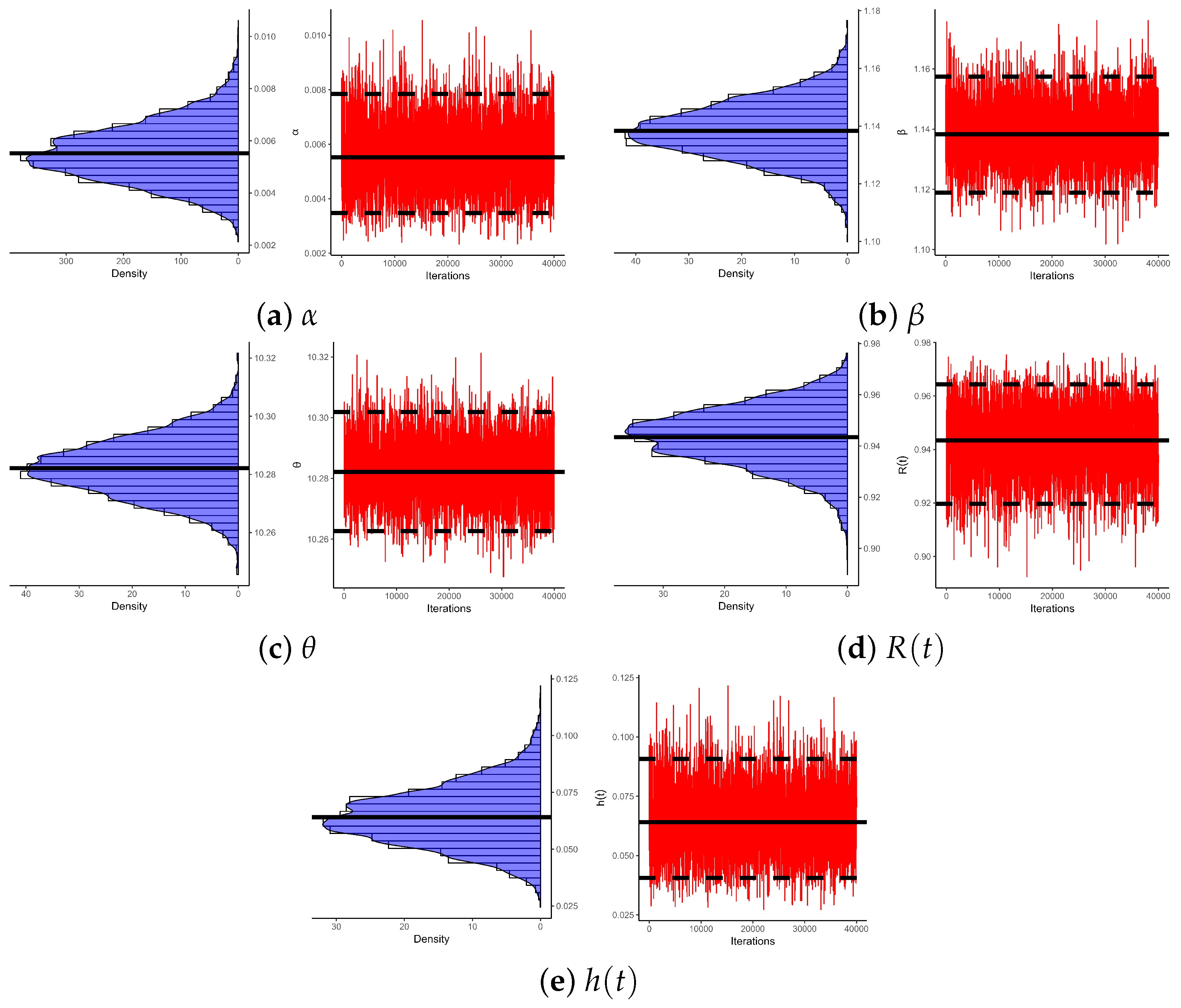
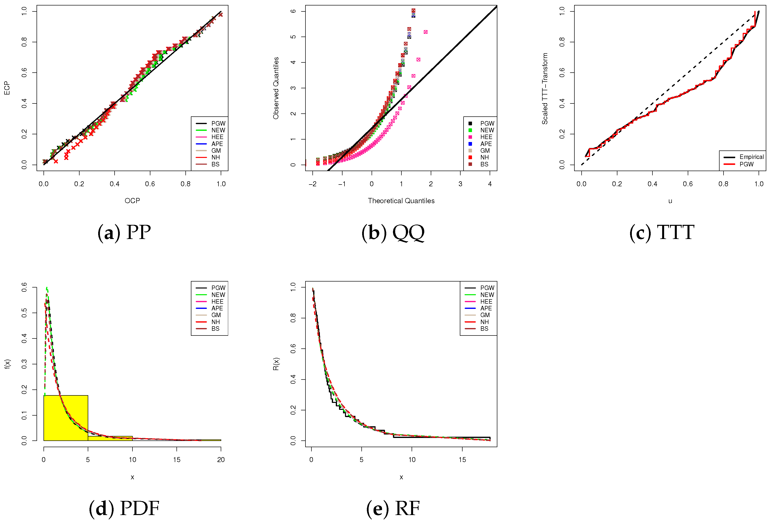
5.1. Bladder Cancer
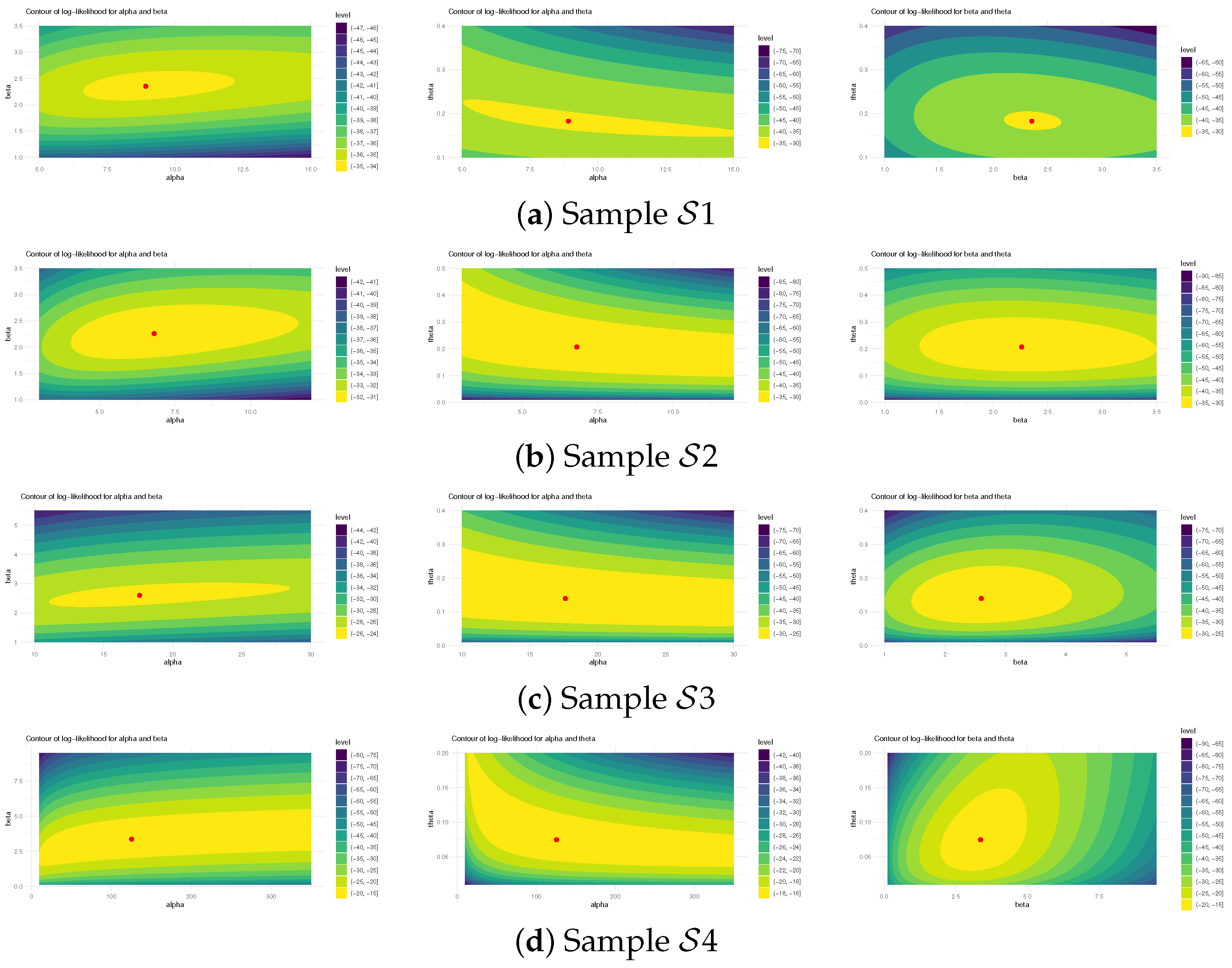
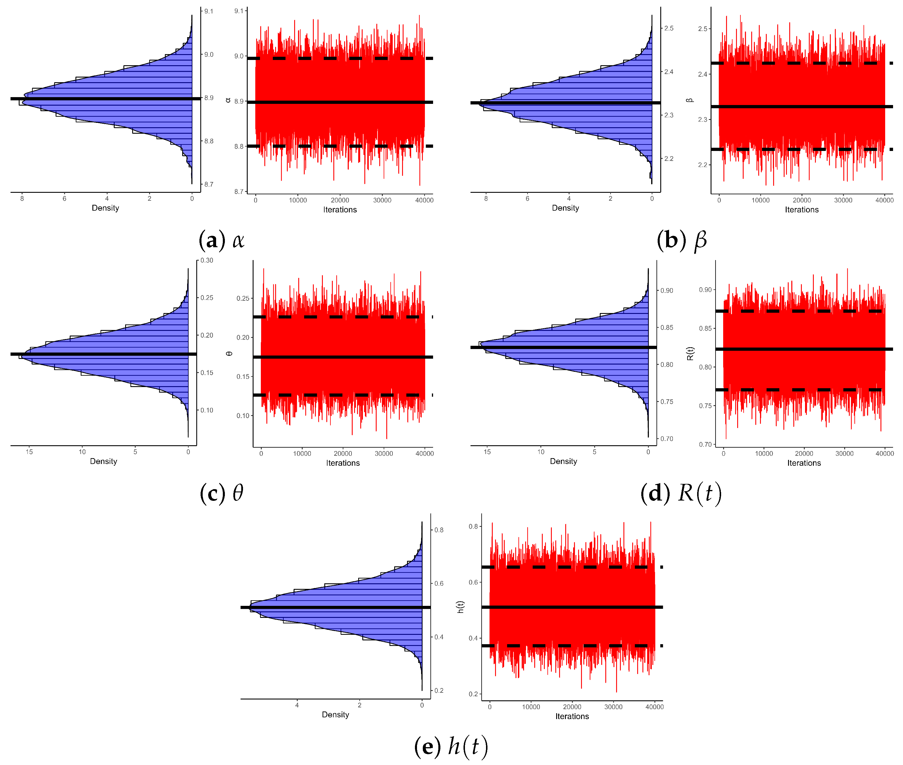
5.2. Head and Neck Cancer
6. Conclusions
Author Contributions
Funding
Data Availability Statement
Conflicts of Interest
References
- Bagdonavi čius, V.; Nikulin, M. Accelerated Life Models: Modeling and Statistical Analysis; Chapman and Hall/CRC: New York, NY, USA, 2001. [Google Scholar]
- Dimitrakopoulou, T.; Adamidis, K.; Loukas, S. A lifetime distribution with an upside-down bathtub-shaped hazard function. IEEE Trans. Reliab. 2007, 56, 308–311. [Google Scholar] [CrossRef]
- Nadarajah, S.; Haghighi, F. An extension of the exponential distribution. Statistics 2011, 45, 543–558. [Google Scholar] [CrossRef]
- Nikulin, M.; Haghighi, F. A Chi-Squared Test for the Generalized Power Weibull Family for the Head-and-Neck Cancer Censored Data. J. Math. Sci. 2006, 133, 1333–1341. [Google Scholar] [CrossRef]
- Nikulin, M.; Haghighi. On the power generalized Weibull family: Model for cancer censored data. Metron 2009, 67, 75–86. [Google Scholar]
- Kumar, D.; Dey, S. Power generalized Weibull distribution based on order statistics. J. Stat. Res. 2017, 51, 61–78. [Google Scholar] [CrossRef]
- El-Din, M.M.; Abd El-Raheem, A.M.; Abd El-Azeem, S.O. On progressive-stress accelerated life testing for power generalized Weibull distribution under progressive type-II censoring. J. Stat. Appl. Probab. Lett. 2018, 5, 131–143. [Google Scholar] [CrossRef]
- Pandey, R.; Kumari, N. Bayesian analysis of power generalized Weibull distribution. Int. J. Appl. Comput. Math. 2018, 4, 1–16. [Google Scholar] [CrossRef]
- Sabry, M.A.; Muhammed, H.Z.; Nabih, A.; Shaaban, M. Parameter estimation for the power generalized Weibull distribution based on one-and two-stage ranked set sampling designs. J. Stat. Appl. Probab. 2019, 8, 113–128. [Google Scholar]
- Dey, S.; Nassar, M.; Ali, S.; Kumar, D.; Raheem, E. Comparison of Estimation Methods of the Power Generalized Weibull Distribution. Statistica 2022, 82, 339–372. [Google Scholar]
- Epstein, B. Truncated life tests in the exponential case. Ann. Math. Stat. 1954, 25, 555–564. [Google Scholar] [CrossRef]
- Childs, A.; Chandrasekar, B.; Balakrishnan, N.; Kundu, D. Exact likelihood inference based on Type-I and Type-II hybrid censored samples from the exponential distribution. Ann. Inst. Stat. Math. 2003, 55, 319–330. [Google Scholar] [CrossRef]
- Chandrasekar, B.; Childs, A.; Balakrishnan, N. Exact likelihood inference for the exponential distribution under generalized Type-I and Type-II hybrid censoring. Nav. Res. Logist. 2004, 51, 994–1004. [Google Scholar] [CrossRef]
- Balakrishnan, N.; Rasouli, A.; Sanjari Farsipour, N. Exact likelihood inference based on an unified hybrid censored sample from the exponential distribution. J. Stat. Comput. Simul. 2008, 78, 475–488. [Google Scholar] [CrossRef]
- Panahi, H.; Sayyareh, A. Estimation and prediction for a unified hybrid-censored Burr Type XII distribution. J. Stat. Comput. Simul. 2016, 86, 55–73. [Google Scholar] [CrossRef]
- Jeon, Y.E.; Kang, S.B. Estimation of the Rayleigh distribution under unified hybrid censoring. Austrian J. Stat. 2021, 50, 59–73. [Google Scholar] [CrossRef]
- Dutta, S.; Kayal, S. Bayesian and non-Bayesian inference of Weibull lifetime model based on partially observed competing risks data under unified hybrid censoring scheme. Qual. Reliab. Eng. Int. 2022, 38, 3867–3891. [Google Scholar] [CrossRef]
- Dutta, S.; Lio, Y.; Kayal, S. Parametric inferences using dependent competing risks data with partially observed failure causes from MOBK distribution under unified hybrid censoring. J. Stat. Comput. Simul. 2024, 94, 376–399. [Google Scholar] [CrossRef]
- Hasaballah, M.M.; Tashkandy, Y.A.; Balogun, O.S.; Bakr, M.E. Statistical inference of unified hybrid censoring scheme for generalized inverted exponential distribution with application to COVID-19 data. AIP Adv. 2024, 14, 045111. [Google Scholar] [CrossRef]
- Shukla, A.K.; Soni, S.; Kumar, K. Statistical inference and prediction in unified hybrid censored power Lindley distribution. Life Cycle Reliab. Saf. Eng. 2025, 14, 183–204. [Google Scholar] [CrossRef]
- Alotaibi, R.; Nassar, M.; Khan, Z.A.; Alajlan, W.A.; Elshahhat, A. Entropy evaluation in inverse Weibull unified hybrid censored data with application to mechanical components and head-neck cancer patients. AIMS Math. 2025, 10, 1085–1115. [Google Scholar] [CrossRef]
- Kundu, D. Bayesian inference and life testing plan for the Weibull distribution in presence of progressive censoring. Technometrics 2008, 50, 144–154. [Google Scholar] [CrossRef]
- Henningsen, A.; Toomet, O. maxLik: A package for maximum likelihood estimation in R. Comput. Stat. 2011, 26, 443–458. [Google Scholar] [CrossRef]
- Plummer, M.; Best, N.; Cowles, K.; Vines, K. CODA: Convergence diagnosis and output analysis for MCMC. R News 2006, 6, 7–11. [Google Scholar]
- Lee, E.T.; Wang, J.W. Statistical Methods for Survival Data Analysis, 3rd ed.; Wiley: New York, NY, USA, 2003. [Google Scholar]
- Alotaibi, R.; Nassar, M.; Khan, Z.A.; Elshahhat, A. Analysis of Weibull progressively first-failure censored data with beta-binomial removals. AIMS Math. 2024, 9, 24109–24142. [Google Scholar] [CrossRef]
- Alotaibi, R.; Nassar, M.; Elshahhat, A. A new extended Pham distribution for modelling cancer data. J. Radiat. Res. Appl. Sci. 2024, 17, 100961. [Google Scholar] [CrossRef]
- Peng, X.; Yan, Z. Estimation and application for a new extended Weibull distribution. Reliab. Eng. Syst. Saf. 2014, 121, 34–42. [Google Scholar] [CrossRef]
- Pinho, L.G.B.; Cordeiro, G.M.; Nobre, J.S. The Harris extended exponential distribution. Commun. Stat.-Theory Methods 2015, 44, 3486–3502. [Google Scholar] [CrossRef]
- Oguntunde, P.E.; Balogun, O.S.; Okagbue, H.I.; Bishop, S.A. The Weibull-exponential distribution: Its properties and applications. J. Appl. Sci. 2015, 15, 1305–1311. [Google Scholar] [CrossRef]
- Marshall, A.W.; Olkin, I. Life Distributions; Springer: New York, NY, USA, 2007. [Google Scholar]
- Mahdavi, A.; Kundu, D. A new method for generating distributions with an application to exponential distribution. Commun. Stat. Theory Methods 2017, 46, 6543–6557. [Google Scholar] [CrossRef]
- Gupta, R.D.; Kundu, D. Generalized exponential distribution: Different method of estimations. J. Stat. Comput. Simul. 2001, 69, 315–337. [Google Scholar] [CrossRef]
- Birnbaum, Z.W.; Saunders, S.C. A probabilistic interpretation of Miner’s rule. SIAM J. Appl. Math. 1968, 16, 637–652. [Google Scholar] [CrossRef]
- Weibull, W. A statistical distribution function of wide applicability. J. Appl. Mech. 1951, 18, 293–297. [Google Scholar] [CrossRef]
- Johnson, N.; Kotz, S.; Balakrishnan, N. Continuous Univariate Distributions, 2nd ed.; John Wiley & Sons: New York, NY, USA, 1994. [Google Scholar]
- Pham, H. A vtub-shaped hazard rate function with applications to system safety. Int. J. Reliab. Appl. 2002, 3, 1–16. [Google Scholar]
- Marinho, P.R.D.; Silva, R.B.; Bourguignon, M.; Cordeiro, G.M.; Nadarajah, S. AdequacyModel: An R package for probability distributions and general purpose optimization. PLoS ONE 2019, 14, e0221487. [Google Scholar] [CrossRef]
- Efron, B. Logistic regression, survival analysis, and the Kaplan-Meier curve. J. Am. Stat. Assoc. 1988, 83, 414–425. [Google Scholar] [CrossRef]
- Elshahhat, A.; Rastogi, M.K. Bayesian Life Analysis of Generalized Chen’s Population Under Progressive Censoring. Pak. J. Stat. Oper. Res. 2022, 18, 675–702. [Google Scholar] [CrossRef]
- Elshahhat, A.; Nassar, M. Analysis of adaptive Type-II progressively hybrid censoring with binomial removals. J. Stat. Comput. Simul. 2023, 93, 1077–1103. [Google Scholar] [CrossRef]


| Case | Condition | Termination Point () | Observed Failures (r) |
|---|---|---|---|
| 1 | |||
| 2 | |||
| 3 | |||
| 4 | |||
| 5 | |||
| 6 |
| n | MLE | MCMC-PA | MCMC-PB | ||||||||
|---|---|---|---|---|---|---|---|---|---|---|---|
| Pop-1 | |||||||||||
| (1,4) | 30 | (10,20) | 0.310 | 1.836 | 2.281 | 0.368 | 0.605 | 1.997 | 0.606 | 0.454 | 0.713 |
| (15,25) | 0.232 | 1.729 | 1.958 | 0.423 | 0.564 | 1.860 | 0.385 | 0.397 | 0.672 | ||
| 60 | (20,40) | 0.188 | 1.548 | 1.713 | 0.387 | 0.343 | 1.517 | 0.281 | 0.191 | 0.485 | |
| (30,50) | 0.159 | 1.432 | 0.810 | 0.456 | 0.126 | 0.800 | 0.342 | 0.091 | 0.269 | ||
| 90 | (30,50) | 0.179 | 1.109 | 0.488 | 0.291 | 0.118 | 0.477 | 0.358 | 0.071 | 0.244 | |
| (50,70) | 0.153 | 0.970 | 0.242 | 0.390 | 0.087 | 0.234 | 0.372 | 0.056 | 0.208 | ||
| (4,8) | 30 | (10,20) | 0.289 | 1.621 | 0.663 | 0.355 | 0.530 | 0.636 | 0.298 | 0.392 | 0.590 |
| (15,25) | 0.367 | 1.500 | 0.586 | 0.413 | 0.433 | 0.582 | 0.379 | 0.299 | 0.503 | ||
| 60 | (20,40) | 0.320 | 1.411 | 0.411 | 0.279 | 0.243 | 0.355 | 0.370 | 0.135 | 0.304 | |
| (30,50) | 0.340 | 1.274 | 0.269 | 0.455 | 0.125 | 0.235 | 0.438 | 0.089 | 0.233 | ||
| 90 | (30,50) | 0.426 | 0.998 | 0.234 | 0.386 | 0.106 | 0.199 | 0.429 | 0.066 | 0.193 | |
| (50,70) | 0.298 | 0.905 | 0.208 | 0.319 | 0.087 | 0.184 | 0.397 | 0.056 | 0.184 | ||
| Pop-2 | |||||||||||
| (0.5,1.5) | 30 | (10,20) | 0.564 | 0.483 | 0.565 | 0.497 | 0.302 | 0.481 | 0.381 | 0.246 | 0.446 |
| (15,25) | 0.523 | 0.467 | 0.543 | 0.392 | 0.255 | 0.462 | 0.464 | 0.168 | 0.428 | ||
| 60 | (20,40) | 0.539 | 0.355 | 0.522 | 0.425 | 0.220 | 0.455 | 0.562 | 0.153 | 0.400 | |
| (30,50) | 0.523 | 0.343 | 0.516 | 0.516 | 0.219 | 0.446 | 0.415 | 0.148 | 0.398 | ||
| 90 | (30,50) | 0.533 | 0.310 | 0.497 | 0.397 | 0.205 | 0.424 | 0.455 | 0.141 | 0.378 | |
| (50,70) | 0.495 | 0.239 | 0.427 | 0.427 | 0.150 | 0.387 | 0.479 | 0.118 | 0.343 | ||
| (1.5,2.5) | 30 | (10,20) | 0.458 | 0.398 | 0.428 | 0.438 | 0.278 | 0.388 | 0.587 | 0.184 | 0.358 |
| (15,25) | 0.372 | 0.376 | 0.411 | 0.379 | 0.239 | 0.359 | 0.410 | 0.168 | 0.343 | ||
| 60 | (20,40) | 0.466 | 0.245 | 0.400 | 0.478 | 0.161 | 0.348 | 0.375 | 0.118 | 0.325 | |
| (30,50) | 0.516 | 0.243 | 0.384 | 0.358 | 0.151 | 0.333 | 0.457 | 0.069 | 0.258 | ||
| 90 | (30,50) | 0.427 | 0.234 | 0.381 | 0.276 | 0.149 | 0.330 | 0.379 | 0.059 | 0.236 | |
| (50,70) | 0.339 | 0.183 | 0.324 | 0.432 | 0.118 | 0.301 | 0.501 | 0.057 | 0.223 | ||
| n | MLE | MCMC-PA | MCMC-PB | ||||||||
|---|---|---|---|---|---|---|---|---|---|---|---|
| Pop-1 | |||||||||||
| (1,4) | 30 | (10,20) | 0.601 | 0.462 | 0.407 | 0.597 | 0.119 | 0.261 | 0.591 | 0.083 | 0.225 |
| (15,25) | 0.517 | 0.404 | 0.332 | 0.629 | 0.083 | 0.223 | 0.629 | 0.072 | 0.213 | ||
| 60 | (20,40) | 0.527 | 0.141 | 0.251 | 0.399 | 0.053 | 0.207 | 0.408 | 0.050 | 0.176 | |
| (30,50) | 0.579 | 0.064 | 0.237 | 0.564 | 0.048 | 0.179 | 0.581 | 0.035 | 0.159 | ||
| 90 | (30,50) | 0.479 | 0.044 | 0.177 | 0.431 | 0.033 | 0.146 | 0.316 | 0.033 | 0.138 | |
| (50,70) | 0.566 | 0.035 | 0.146 | 0.628 | 0.028 | 0.132 | 0.563 | 0.020 | 0.097 | ||
| (4,8) | 30 | (10,20) | 0.398 | 0.403 | 0.340 | 0.722 | 0.094 | 0.239 | 0.708 | 0.070 | 0.209 |
| (15,25) | 0.423 | 0.326 | 0.331 | 0.570 | 0.081 | 0.219 | 0.696 | 0.068 | 0.207 | ||
| 60 | (20,40) | 0.463 | 0.139 | 0.233 | 0.486 | 0.050 | 0.200 | 0.495 | 0.048 | 0.171 | |
| (30,50) | 0.513 | 0.051 | 0.198 | 0.642 | 0.048 | 0.176 | 0.642 | 0.033 | 0.153 | ||
| 90 | (30,50) | 0.362 | 0.043 | 0.173 | 0.462 | 0.033 | 0.146 | 0.616 | 0.030 | 0.136 | |
| (50,70) | 0.457 | 0.033 | 0.146 | 0.563 | 0.028 | 0.128 | 0.629 | 0.020 | 0.097 | ||
| Pop-2 | |||||||||||
| (0.5,1.5) | 30 | (10,20) | 0.853 | 0.317 | 0.560 | 0.920 | 0.289 | 0.532 | 0.913 | 0.255 | 0.499 |
| (15,25) | 0.670 | 0.285 | 0.531 | 0.967 | 0.260 | 0.501 | 0.876 | 0.157 | 0.384 | ||
| 60 | (20,40) | 0.707 | 0.287 | 0.529 | 0.880 | 0.247 | 0.491 | 0.959 | 0.152 | 0.374 | |
| (30,50) | 0.796 | 0.277 | 0.520 | 0.930 | 0.246 | 0.487 | 0.783 | 0.133 | 0.346 | ||
| 90 | (30,50) | 0.840 | 0.231 | 0.462 | 0.860 | 0.197 | 0.422 | 0.729 | 0.123 | 0.324 | |
| (50,70) | 0.897 | 0.205 | 0.433 | 0.730 | 0.187 | 0.413 | 0.899 | 0.099 | 0.280 | ||
| (1.5,2.5) | 30 | (10,20) | 0.985 | 0.297 | 0.540 | 0.911 | 0.285 | 0.531 | 0.843 | 0.248 | 0.491 |
| (15,25) | 0.927 | 0.271 | 0.512 | 0.755 | 0.168 | 0.403 | 0.928 | 0.151 | 0.376 | ||
| 60 | (20,40) | 0.839 | 0.257 | 0.499 | 0.843 | 0.164 | 0.396 | 0.754 | 0.143 | 0.363 | |
| (30,50) | 0.762 | 0.255 | 0.498 | 0.745 | 0.148 | 0.374 | 0.897 | 0.125 | 0.335 | ||
| 90 | (30,50) | 0.897 | 0.214 | 0.441 | 0.771 | 0.126 | 0.326 | 0.817 | 0.112 | 0.305 | |
| (50,70) | 0.820 | 0.204 | 0.433 | 0.995 | 0.103 | 0.289 | 0.942 | 0.088 | 0.263 | ||
| n | MLE | MCMC-PA | MCMC-PB | ||||||||
|---|---|---|---|---|---|---|---|---|---|---|---|
| Pop-1 | |||||||||||
| (1,4) | 30 | (10,20) | 0.717 | 1.264 | 1.387 | 0.757 | 0.796 | 0.804 | 0.699 | 0.629 | 0.721 |
| (15,25) | 0.692 | 1.229 | 1.261 | 0.828 | 0.754 | 0.767 | 0.994 | 0.541 | 0.666 | ||
| 60 | (20,40) | 0.762 | 1.177 | 1.168 | 0.732 | 0.528 | 0.599 | 0.760 | 0.407 | 0.510 | |
| (30,50) | 0.712 | 1.167 | 1.004 | 0.911 | 0.319 | 0.495 | 0.749 | 0.255 | 0.425 | ||
| 90 | (30,50) | 0.839 | 0.999 | 0.931 | 0.881 | 0.294 | 0.453 | 0.632 | 0.218 | 0.397 | |
| (50,70) | 0.762 | 0.841 | 0.820 | 0.792 | 0.253 | 0.424 | 0.878 | 0.206 | 0.376 | ||
| (4,8) | 30 | (10,20) | 0.741 | 1.229 | 1.176 | 0.698 | 0.766 | 0.733 | 0.704 | 0.579 | 0.707 |
| (15,25) | 0.916 | 1.198 | 1.134 | 0.725 | 0.726 | 0.709 | 0.982 | 0.509 | 0.639 | ||
| 60 | (20,40) | 0.889 | 1.169 | 1.026 | 0.618 | 0.467 | 0.582 | 0.847 | 0.328 | 0.481 | |
| (30,50) | 0.752 | 1.072 | 0.940 | 0.791 | 0.310 | 0.482 | 0.993 | 0.225 | 0.414 | ||
| 90 | (30,50) | 0.780 | 0.957 | 0.890 | 0.844 | 0.279 | 0.432 | 0.712 | 0.208 | 0.372 | |
| (50,70) | 0.814 | 0.747 | 0.741 | 0.905 | 0.249 | 0.395 | 0.931 | 0.197 | 0.353 | ||
| Pop-2 | |||||||||||
| (0.5,1.5) | 30 | (10,20) | 1.177 | 1.672 | 1.418 | 1.094 | 0.647 | 0.832 | 1.359 | 0.633 | 0.772 |
| (15,25) | 1.027 | 1.461 | 1.328 | 1.278 | 0.633 | 0.798 | 1.402 | 0.610 | 0.681 | ||
| 60 | (20,40) | 1.376 | 1.356 | 1.238 | 1.386 | 0.620 | 0.716 | 1.215 | 0.508 | 0.616 | |
| (30,50) | 1.429 | 1.250 | 1.115 | 1.246 | 0.595 | 0.698 | 1.390 | 0.487 | 0.603 | ||
| 90 | (30,50) | 1.202 | 1.211 | 0.982 | 1.492 | 0.514 | 0.638 | 1.245 | 0.412 | 0.523 | |
| (50,70) | 1.352 | 1.183 | 0.876 | 1.106 | 0.492 | 0.604 | 1.529 | 0.390 | 0.497 | ||
| (1.5,2.5) | 30 | (10,20) | 1.485 | 0.646 | 1.261 | 1.486 | 0.646 | 0.800 | 1.017 | 0.614 | 0.745 |
| (15,25) | 1.185 | 0.627 | 1.026 | 1.268 | 0.624 | 0.708 | 1.189 | 0.554 | 0.668 | ||
| 60 | (20,40) | 0.986 | 0.611 | 0.956 | 1.591 | 0.590 | 0.659 | 1.449 | 0.482 | 0.599 | |
| (30,50) | 1.352 | 0.596 | 0.944 | 1.278 | 0.584 | 0.651 | 1.301 | 0.467 | 0.585 | ||
| 90 | (30,50) | 1.426 | 0.579 | 0.870 | 1.058 | 0.498 | 0.600 | 1.291 | 0.373 | 0.517 | |
| (50,70) | 1.286 | 0.538 | 0.850 | 1.377 | 0.472 | 0.586 | 1.467 | 0.344 | 0.497 | ||
| n | MLE | MCMC-PA | MCMC-PB | ||||||||
|---|---|---|---|---|---|---|---|---|---|---|---|
| Pop-1 | |||||||||||
| (1,4) | 30 | (10,20) | 0.957 | 0.190 | 0.426 | 0.967 | 0.153 | 0.385 | 0.929 | 0.117 | 0.373 |
| (15,25) | 0.941 | 0.125 | 0.317 | 0.940 | 0.114 | 0.323 | 0.936 | 0.067 | 0.306 | ||
| 60 | (20,40) | 0.964 | 0.063 | 0.196 | 0.930 | 0.051 | 0.189 | 0.965 | 0.016 | 0.170 | |
| (30,50) | 0.979 | 0.014 | 0.077 | 0.969 | 0.012 | 0.083 | 0.982 | 0.011 | 0.077 | ||
| 90 | (30,50) | 0.926 | 0.009 | 0.067 | 0.957 | 0.007 | 0.057 | 0.958 | 0.006 | 0.055 | |
| (50,70) | 0.943 | 0.007 | 0.057 | 0.942 | 0.006 | 0.064 | 0.973 | 0.006 | 0.056 | ||
| (4,8) | 30 | (10,20) | 0.968 | 0.163 | 0.367 | 0.961 | 0.141 | 0.328 | 0.957 | 0.109 | 0.316 |
| (15,25) | 0.974 | 0.122 | 0.242 | 0.965 | 0.074 | 0.233 | 0.941 | 0.059 | 0.219 | ||
| 60 | (20,40) | 0.971 | 0.062 | 0.096 | 0.946 | 0.019 | 0.102 | 0.963 | 0.014 | 0.089 | |
| (30,50) | 0.964 | 0.013 | 0.075 | 0.956 | 0.011 | 0.081 | 0.954 | 0.010 | 0.076 | ||
| 90 | (30,50) | 0.959 | 0.008 | 0.067 | 0.965 | 0.007 | 0.057 | 0.964 | 0.006 | 0.054 | |
| (50,70) | 0.943 | 0.007 | 0.052 | 0.948 | 0.006 | 0.059 | 0.944 | 0.006 | 0.051 | ||
| Pop-2 | |||||||||||
| (0.5,1.5) | 30 | (10,20) | 0.935 | 0.213 | 0.460 | 0.919 | 0.195 | 0.447 | 0.932 | 0.158 | 0.438 |
| (15,25) | 0.931 | 0.199 | 0.442 | 0.921 | 0.177 | 0.428 | 0.932 | 0.089 | 0.415 | ||
| 60 | (20,40) | 0.915 | 0.185 | 0.419 | 0.928 | 0.161 | 0.394 | 0.924 | 0.085 | 0.384 | |
| (30,50) | 0.921 | 0.177 | 0.428 | 0.932 | 0.151 | 0.409 | 0.927 | 0.076 | 0.395 | ||
| 90 | (30,50) | 0.925 | 0.167 | 0.408 | 0.923 | 0.137 | 0.381 | 0.919 | 0.074 | 0.357 | |
| (50,70) | 0.931 | 0.145 | 0.372 | 0.932 | 0.120 | 0.360 | 0.920 | 0.058 | 0.335 | ||
| (1.5,2.5) | 30 | (10,20) | 0.932 | 0.202 | 0.419 | 0.931 | 0.177 | 0.394 | 0.936 | 0.151 | 0.385 |
| (15,25) | 0.918 | 0.188 | 0.301 | 0.927 | 0.094 | 0.289 | 0.929 | 0.081 | 0.286 | ||
| 60 | (20,40) | 0.922 | 0.171 | 0.295 | 0.930 | 0.090 | 0.266 | 0.933 | 0.080 | 0.275 | |
| (30,50) | 0.919 | 0.158 | 0.280 | 0.924 | 0.083 | 0.283 | 0.918 | 0.070 | 0.254 | ||
| 90 | (30,50) | 0.926 | 0.154 | 0.267 | 0.935 | 0.079 | 0.254 | 0.929 | 0.063 | 0.233 | |
| (50,70) | 0.934 | 0.138 | 0.233 | 0.923 | 0.064 | 0.217 | 0.935 | 0.049 | 0.198 | ||
| n | MLE | MCMC-PA | MCMC-PB | ||||||||
|---|---|---|---|---|---|---|---|---|---|---|---|
| Pop-1 | |||||||||||
| (1,4) | 30 | (10,20) | 0.421 | 1.307 | 1.094 | 0.279 | 0.882 | 0.919 | 0.480 | 0.820 | 0.864 |
| (15,25) | 0.539 | 1.089 | 0.962 | 0.387 | 0.875 | 0.905 | 0.540 | 0.717 | 0.816 | ||
| 60 | (20,40) | 0.470 | 0.741 | 0.824 | 0.482 | 0.597 | 0.660 | 0.392 | 0.432 | 0.548 | |
| (30,50) | 0.357 | 0.281 | 0.433 | 0.295 | 0.262 | 0.419 | 0.429 | 0.242 | 0.403 | ||
| 90 | (30,50) | 0.413 | 0.218 | 0.385 | 0.277 | 0.212 | 0.340 | 0.285 | 0.179 | 0.321 | |
| (50,70) | 0.393 | 0.175 | 0.365 | 0.187 | 0.152 | 0.332 | 0.346 | 0.142 | 0.315 | ||
| (4,8) | 30 | (10,20) | 0.371 | 1.134 | 0.980 | 0.469 | 0.872 | 0.915 | 0.639 | 0.803 | 0.856 |
| (15,25) | 0.470 | 0.966 | 0.922 | 0.548 | 0.829 | 0.879 | 0.525 | 0.710 | 0.807 | ||
| 60 | (20,40) | 0.331 | 0.646 | 0.692 | 0.419 | 0.592 | 0.649 | 0.420 | 0.374 | 0.512 | |
| (30,50) | 0.286 | 0.280 | 0.433 | 0.365 | 0.261 | 0.419 | 0.463 | 0.241 | 0.402 | ||
| 90 | (30,50) | 0.200 | 0.216 | 0.351 | 0.330 | 0.185 | 0.335 | 0.386 | 0.157 | 0.306 | |
| (50,70) | 0.302 | 0.175 | 0.344 | 0.223 | 0.152 | 0.327 | 0.316 | 0.142 | 0.311 | ||
| Pop-2 | |||||||||||
| (0.5,1.5) | 30 | (10,20) | 1.327 | 0.855 | 0.904 | 1.331 | 0.767 | 0.838 | 1.373 | 0.735 | 0.805 |
| (15,25) | 1.400 | 0.781 | 0.868 | 1.336 | 0.730 | 0.814 | 1.369 | 0.724 | 0.762 | ||
| 60 | (20,40) | 1.136 | 0.739 | 0.851 | 1.162 | 0.703 | 0.807 | 1.206 | 0.501 | 0.639 | |
| (30,50) | 1.173 | 0.724 | 0.824 | 1.209 | 0.673 | 0.781 | 1.248 | 0.473 | 0.594 | ||
| 90 | (30,50) | 1.027 | 0.670 | 0.811 | 1.084 | 0.651 | 0.771 | 1.117 | 0.460 | 0.636 | |
| (50,70) | 1.137 | 0.501 | 0.664 | 1.211 | 0.388 | 0.567 | 1.236 | 0.354 | 0.524 | ||
| (1.5,2.5) | 30 | (10,20) | 0.715 | 0.785 | 0.841 | 0.686 | 0.737 | 0.829 | 0.774 | 0.731 | 0.767 |
| (15,25) | 0.576 | 0.732 | 0.837 | 0.706 | 0.726 | 0.799 | 0.651 | 0.704 | 0.727 | ||
| 60 | (20,40) | 0.622 | 0.713 | 0.816 | 0.644 | 0.545 | 0.678 | 0.481 | 0.446 | 0.604 | |
| (30,50) | 0.496 | 0.689 | 0.803 | 0.572 | 0.519 | 0.665 | 0.586 | 0.415 | 0.568 | ||
| 90 | (30,50) | 0.537 | 0.670 | 0.790 | 0.510 | 0.504 | 0.641 | 0.474 | 0.370 | 0.567 | |
| (50,70) | 0.596 | 0.472 | 0.639 | 0.547 | 0.370 | 0.553 | 0.518 | 0.268 | 0.457 | ||
| n | ACI | BCI-PA | BCI-PB | |||||
|---|---|---|---|---|---|---|---|---|
| Pop-1 | ||||||||
| (1,4) | 30 | (10,20) | 3.741 | 0.877 | 3.253 | 0.884 | 3.009 | 0.893 |
| (15,25) | 3.218 | 0.882 | 2.763 | 0.889 | 2.556 | 0.897 | ||
| 60 | (20,40) | 2.944 | 0.885 | 2.572 | 0.893 | 2.379 | 0.900 | |
| (30,50) | 2.541 | 0.902 | 2.284 | 0.910 | 2.112 | 0.918 | ||
| 90 | (30,50) | 2.375 | 0.905 | 2.108 | 0.913 | 1.950 | 0.920 | |
| (50,70) | 1.989 | 0.912 | 1.885 | 0.917 | 1.744 | 0.922 | ||
| (4,8) | 30 | (10,20) | 0.700 | 0.914 | 0.602 | 0.920 | 0.589 | 0.927 |
| (15,25) | 0.658 | 0.919 | 0.596 | 0.926 | 0.584 | 0.931 | ||
| 60 | (20,40) | 0.590 | 0.923 | 0.583 | 0.929 | 0.555 | 0.934 | |
| (30,50) | 0.493 | 0.938 | 0.491 | 0.947 | 0.488 | 0.952 | ||
| 90 | (30,50) | 0.470 | 0.943 | 0.440 | 0.950 | 0.440 | 0.953 | |
| (50,70) | 0.406 | 0.948 | 0.384 | 0.954 | 0.384 | 0.957 | ||
| Pop-2 | ||||||||
| (0.5,1.5) | 30 | (10,20) | 2.678 | 0.884 | 2.422 | 0.892 | 2.241 | 0.900 |
| (15,25) | 2.499 | 0.889 | 2.376 | 0.897 | 2.198 | 0.905 | ||
| 60 | (20,40) | 2.254 | 0.902 | 2.145 | 0.910 | 1.984 | 0.917 | |
| (30,50) | 2.148 | 0.904 | 1.872 | 0.912 | 1.732 | 0.920 | ||
| 90 | (30,50) | 1.955 | 0.908 | 1.645 | 0.916 | 1.522 | 0.922 | |
| (50,70) | 1.645 | 0.914 | 1.491 | 0.920 | 1.380 | 0.925 | ||
| (1.5,2.5) | 30 | (10,20) | 0.702 | 0.922 | 0.652 | 0.928 | 0.598 | 0.934 |
| (15,25) | 0.683 | 0.927 | 0.629 | 0.933 | 0.589 | 0.939 | ||
| 60 | (20,40) | 0.650 | 0.940 | 0.588 | 0.947 | 0.531 | 0.951 | |
| (30,50) | 0.641 | 0.942 | 0.582 | 0.949 | 0.521 | 0.955 | ||
| 90 | (30,50) | 0.633 | 0.947 | 0.536 | 0.953 | 0.513 | 0.956 | |
| (50,70) | 0.590 | 0.951 | 0.512 | 0.957 | 0.475 | 0.959 | ||
| n | ACI | BCI-PA | BCI-PB | |||||
|---|---|---|---|---|---|---|---|---|
| Pop-1 | ||||||||
| (1,4) | 30 | (10,20) | 1.282 | 0.913 | 0.581 | 0.920 | 0.515 | 0.922 |
| (15,25) | 1.178 | 0.916 | 0.519 | 0.923 | 0.500 | 0.925 | ||
| 60 | (20,40) | 0.965 | 0.919 | 0.372 | 0.926 | 0.355 | 0.928 | |
| (30,50) | 0.706 | 0.925 | 0.337 | 0.932 | 0.316 | 0.934 | ||
| 90 | (30,50) | 0.619 | 0.930 | 0.309 | 0.937 | 0.270 | 0.940 | |
| (50,70) | 0.497 | 0.936 | 0.203 | 0.943 | 0.179 | 0.946 | ||
| (4,8) | 30 | (10,20) | 1.173 | 0.916 | 0.524 | 0.922 | 0.496 | 0.924 |
| (15,25) | 0.987 | 0.919 | 0.510 | 0.925 | 0.459 | 0.927 | ||
| 60 | (20,40) | 0.833 | 0.922 | 0.357 | 0.928 | 0.335 | 0.930 | |
| (30,50) | 0.694 | 0.928 | 0.329 | 0.934 | 0.297 | 0.936 | ||
| 90 | (30,50) | 0.497 | 0.933 | 0.297 | 0.939 | 0.262 | 0.941 | |
| (50,70) | 0.459 | 0.939 | 0.196 | 0.945 | 0.167 | 0.947 | ||
| Pop-2 | ||||||||
| (0.5,1.5) | 30 | (10,20) | 0.535 | 0.924 | 0.363 | 0.931 | 0.271 | 0.933 |
| (15,25) | 0.458 | 0.928 | 0.335 | 0.935 | 0.268 | 0.937 | ||
| 60 | (20,40) | 0.257 | 0.936 | 0.223 | 0.943 | 0.185 | 0.945 | |
| (30,50) | 0.225 | 0.938 | 0.213 | 0.945 | 0.166 | 0.947 | ||
| 90 | (30,50) | 0.191 | 0.941 | 0.172 | 0.947 | 0.138 | 0.950 | |
| (50,70) | 0.143 | 0.943 | 0.136 | 0.949 | 0.125 | 0.952 | ||
| (1.5,2.5) | 30 | (10,20) | 0.417 | 0.927 | 0.351 | 0.933 | 0.225 | 0.935 |
| (15,25) | 0.370 | 0.931 | 0.327 | 0.937 | 0.206 | 0.939 | ||
| 60 | (20,40) | 0.229 | 0.939 | 0.191 | 0.945 | 0.177 | 0.947 | |
| (30,50) | 0.218 | 0.941 | 0.179 | 0.947 | 0.160 | 0.949 | ||
| 90 | (30,50) | 0.176 | 0.944 | 0.143 | 0.949 | 0.132 | 0.952 | |
| (50,70) | 0.138 | 0.946 | 0.130 | 0.952 | 0.122 | 0.954 | ||
| n | ACI | BCI-PA | BCI-PB | |||||
|---|---|---|---|---|---|---|---|---|
| Pop-1 | ||||||||
| (1,4) | 30 | (10,20) | 2.193 | 0.892 | 1.423 | 0.905 | 0.852 | 0.914 |
| (15,25) | 2.016 | 0.893 | 1.407 | 0.909 | 0.827 | 0.916 | ||
| 60 | (20,40) | 1.889 | 0.896 | 1.328 | 0.912 | 0.810 | 0.919 | |
| (30,50) | 1.641 | 0.900 | 1.276 | 0.916 | 0.786 | 0.923 | ||
| 90 | (30,50) | 1.476 | 0.904 | 1.200 | 0.920 | 0.746 | 0.927 | |
| (50,70) | 1.378 | 0.907 | 0.973 | 0.923 | 0.738 | 0.928 | ||
| (4,8) | 30 | (10,20) | 1.938 | 0.901 | 1.244 | 0.908 | 0.823 | 0.918 |
| (15,25) | 1.748 | 0.905 | 1.152 | 0.912 | 0.810 | 0.920 | ||
| 60 | (20,40) | 1.630 | 0.908 | 1.037 | 0.915 | 0.795 | 0.923 | |
| (30,50) | 1.403 | 0.912 | 1.007 | 0.919 | 0.761 | 0.927 | ||
| 90 | (30,50) | 1.356 | 0.916 | 1.000 | 0.923 | 0.725 | 0.931 | |
| (50,70) | 1.223 | 0.919 | 0.973 | 0.926 | 0.687 | 0.934 | ||
| Pop-2 | ||||||||
| (0.5,1.5) | 30 | (10,20) | 2.343 | 0.886 | 1.573 | 0.899 | 0.964 | 0.907 |
| (15,25) | 2.109 | 0.891 | 1.469 | 0.904 | 0.892 | 0.911 | ||
| 60 | (20,40) | 1.991 | 0.894 | 1.359 | 0.907 | 0.844 | 0.914 | |
| (30,50) | 1.671 | 0.899 | 1.279 | 0.912 | 0.827 | 0.919 | ||
| 90 | (30,50) | 1.513 | 0.902 | 1.211 | 0.915 | 0.817 | 0.922 | |
| (50,70) | 1.403 | 0.905 | 1.177 | 0.918 | 0.806 | 0.924 | ||
| (1.5,2.5) | 30 | (10,20) | 2.126 | 0.895 | 1.394 | 0.902 | 0.883 | 0.911 |
| (15,25) | 1.988 | 0.900 | 1.344 | 0.907 | 0.849 | 0.915 | ||
| 60 | (20,40) | 1.757 | 0.903 | 1.287 | 0.910 | 0.827 | 0.918 | |
| (30,50) | 1.597 | 0.908 | 1.218 | 0.915 | 0.813 | 0.923 | ||
| 90 | (30,50) | 1.403 | 0.911 | 1.177 | 0.918 | 0.781 | 0.926 | |
| (50,70) | 1.321 | 0.914 | 1.146 | 0.921 | 0.779 | 0.929 | ||
| n | ACI | BCI-PA | BCI-PB | |||||
|---|---|---|---|---|---|---|---|---|
| Pop-1 | ||||||||
| (1,4) | 30 | (10,20) | 0.299 | 0.932 | 0.220 | 0.937 | 0.189 | 0.941 |
| (15,25) | 0.246 | 0.935 | 0.208 | 0.940 | 0.168 | 0.944 | ||
| 60 | (20,40) | 0.183 | 0.938 | 0.167 | 0.943 | 0.155 | 0.946 | |
| (30,50) | 0.173 | 0.939 | 0.149 | 0.944 | 0.141 | 0.948 | ||
| 90 | (30,50) | 0.163 | 0.940 | 0.139 | 0.945 | 0.127 | 0.949 | |
| (50,70) | 0.128 | 0.942 | 0.116 | 0.947 | 0.110 | 0.951 | ||
| (4,8) | 30 | (10,20) | 0.259 | 0.934 | 0.199 | 0.940 | 0.186 | 0.943 |
| (15,25) | 0.226 | 0.937 | 0.179 | 0.943 | 0.161 | 0.946 | ||
| 60 | (20,40) | 0.178 | 0.940 | 0.158 | 0.946 | 0.152 | 0.949 | |
| (30,50) | 0.163 | 0.941 | 0.147 | 0.947 | 0.139 | 0.950 | ||
| 90 | (30,50) | 0.154 | 0.942 | 0.133 | 0.948 | 0.121 | 0.951 | |
| (50,70) | 0.122 | 0.944 | 0.112 | 0.949 | 0.097 | 0.953 | ||
| Pop-2 | ||||||||
| (0.5,1.5) | 30 | (10,20) | 0.233 | 0.936 | 0.214 | 0.941 | 0.203 | 0.945 |
| (15,25) | 0.229 | 0.937 | 0.203 | 0.942 | 0.197 | 0.946 | ||
| 60 | (20,40) | 0.176 | 0.942 | 0.152 | 0.947 | 0.142 | 0.951 | |
| (30,50) | 0.163 | 0.944 | 0.145 | 0.949 | 0.137 | 0.953 | ||
| 90 | (30,50) | 0.132 | 0.948 | 0.127 | 0.952 | 0.118 | 0.955 | |
| (50,70) | 0.129 | 0.949 | 0.120 | 0.953 | 0.106 | 0.956 | ||
| (1.5,2.5) | 30 | (10,20) | 0.221 | 0.938 | 0.203 | 0.944 | 0.199 | 0.946 |
| (15,25) | 0.213 | 0.939 | 0.199 | 0.945 | 0.191 | 0.948 | ||
| 60 | (20,40) | 0.165 | 0.944 | 0.144 | 0.950 | 0.139 | 0.952 | |
| (30,50) | 0.152 | 0.946 | 0.140 | 0.952 | 0.123 | 0.955 | ||
| 90 | (30,50) | 0.133 | 0.950 | 0.122 | 0.954 | 0.116 | 0.957 | |
| (50,70) | 0.129 | 0.951 | 0.110 | 0.955 | 0.094 | 0.959 | ||
| n | ACI | BCI-PA | BCI-PB | |||||
|---|---|---|---|---|---|---|---|---|
| Pop-1 | ||||||||
| (1,4) | 30 | (10,20) | 1.251 | 0.922 | 0.735 | 0.927 | 0.710 | 0.929 |
| (15,25) | 1.137 | 0.926 | 0.597 | 0.930 | 0.565 | 0.933 | ||
| 60 | (20,40) | 0.821 | 0.930 | 0.561 | 0.933 | 0.487 | 0.935 | |
| (30,50) | 0.808 | 0.932 | 0.495 | 0.935 | 0.434 | 0.937 | ||
| 90 | (30,50) | 0.617 | 0.935 | 0.452 | 0.937 | 0.417 | 0.940 | |
| (50,70) | 0.498 | 0.938 | 0.396 | 0.941 | 0.356 | 0.943 | ||
| (4,8) | 30 | (10,20) | 1.163 | 0.925 | 0.712 | 0.928 | 0.662 | 0.930 |
| (15,25) | 1.085 | 0.929 | 0.570 | 0.931 | 0.556 | 0.934 | ||
| 60 | (20,40) | 0.816 | 0.933 | 0.552 | 0.934 | 0.469 | 0.936 | |
| (30,50) | 0.727 | 0.935 | 0.446 | 0.936 | 0.430 | 0.938 | ||
| 90 | (30,50) | 0.604 | 0.938 | 0.434 | 0.938 | 0.397 | 0.941 | |
| (50,70) | 0.424 | 0.941 | 0.361 | 0.942 | 0.346 | 0.944 | ||
| Pop-2 | ||||||||
| (0.5,1.5) | 30 | (10,20) | 1.000 | 0.927 | 0.832 | 0.929 | 0.686 | 0.931 |
| (15,25) | 0.945 | 0.928 | 0.786 | 0.931 | 0.677 | 0.932 | ||
| 60 | (20,40) | 0.765 | 0.932 | 0.660 | 0.934 | 0.495 | 0.934 | |
| (30,50) | 0.643 | 0.934 | 0.584 | 0.935 | 0.479 | 0.937 | ||
| 90 | (30,50) | 0.512 | 0.936 | 0.492 | 0.937 | 0.467 | 0.938 | |
| (50,70) | 0.424 | 0.939 | 0.464 | 0.940 | 0.389 | 0.943 | ||
| (1.5,2.5) | 30 | (10,20) | 0.835 | 0.930 | 0.811 | 0.930 | 0.678 | 0.932 |
| (15,25) | 0.813 | 0.931 | 0.761 | 0.932 | 0.670 | 0.933 | ||
| 60 | (20,40) | 0.605 | 0.935 | 0.544 | 0.935 | 0.487 | 0.935 | |
| (30,50) | 0.594 | 0.937 | 0.528 | 0.936 | 0.468 | 0.938 | ||
| 90 | (30,50) | 0.498 | 0.939 | 0.479 | 0.938 | 0.456 | 0.939 | |
| (50,70) | 0.467 | 0.942 | 0.421 | 0.941 | 0.365 | 0.944 | ||
| 0.08 | 0.20 | 0.40 | 0.50 | 0.51 | 0.81 | 0.90 | 1.05 | 1.19 | 1.26 | 1.35 | 1.40 |
| 1.46 | 1.76 | 2.02 | 2.02 | 2.07 | 2.09 | 2.23 | 2.26 | 2.46 | 2.54 | 2.62 | 2.64 |
| 2.69 | 2.69 | 2.75 | 2.83 | 2.87 | 3.02 | 3.25 | 3.31 | 3.36 | 3.36 | 3.48 | 3.52 |
| 3.57 | 3.64 | 3.70 | 3.82 | 3.88 | 4.18 | 4.23 | 4.26 | 4.33 | 4.34 | 4.40 | 4.50 |
| 4.51 | 4.87 | 4.98 | 5.06 | 5.09 | 5.17 | 5.32 | 5.32 | 5.34 | 5.41 | 5.41 | 5.49 |
| 5.62 | 5.71 | 5.85 | 6.25 | 6.54 | 6.76 | 6.93 | 6.94 | 6.97 | 7.09 | 7.26 | 7.28 |
| 7.32 | 7.39 | 7.59 | 7.62 | 7.63 | 7.66 | 7.87 | 7.93 | 8.26 | 8.37 | 8.53 | 8.65 |
| 8.66 | 9.02 | 9.22 | 9.47 | 9.74 | 10.06 | 10.34 | 10.66 | 10.75 | 11.25 | 11.64 | 11.79 |
| 11.98 | 12.02 | 12.03 | 12.07 | 12.63 | 13.11 | 13.29 | 13.80 | 14.24 | 14.76 | 14.77 | 14.83 |
| 15.96 | 16.62 | 17.12 | 17.14 | 17.36 | 18.10 | 19.13 | 20.28 | 21.73 | 22.69 | 23.63 | 25.74 |
| 25.82 | 26.31 | 32.15 | 34.26 | 36.66 | 43.01 | 46.12 | 79.05 |
| Model | Symbol | Author(s) |
|---|---|---|
| New Extended Weibull | NEW | Peng and Yan [28] |
| Harris Extended Exponential | HEE | Pinho et al. [29] |
| Weibull Exponential | WE | Oguntunde et al. [30] |
| Gompertz–Makeham | GM | Marshall and Olkin [31] |
| Alpha Power Exponential | APE | Mahdavi and Kundu [32] |
| Nadarajah–Haghighi | NH | Nadarajah and Haghighi [3] |
| Generalized Exponential | GE | Gupta and Kundu [33] |
| Birnbaum–Saunders | BS | Birnbaum and Saunders [34] |
| Weibull | W | Weibull [35] |
| Gamma | G | Johnson et al. [36] |
| Pham | P | Pham [37] |
| Model | A.I | CA.I | A–D | N-LL | K–S | p-Value | ||||||
|---|---|---|---|---|---|---|---|---|---|---|---|---|
| Est. | Std.Err | Est. | Std.Err | Est. | Std.Err | B.I | HQ.I | CvM | ||||
| PGW | 0.142 | 0.039 | 1.557 | 0.241 | 0.422 | 0.109 | 826.60 | 826.80 | 0.235 | 410.30 | 0.039 | 0.990 |
| 835.16 | 830.08 | 0.035 | ||||||||||
| NEW | 0.127 | 0.150 | 1.020 | 0.074 | 0.103 | 0.023 | 833.12 | 833.31 | 0.742 | 413.56 | 0.070 | 0.561 |
| 841.67 | 836.60 | 0.121 | ||||||||||
| HEE | 0.244 | 0.474 | 0.134 | 0.073 | 1.170 | 0.573 | 833.27 | 833.46 | 0.454 | 413.63 | 0.096 | 0.192 |
| 841.82 | 836.74 | 0.075 | ||||||||||
| WE | 12.805 | 5.003 | 0.985 | 0.063 | 0.007 | 0.002 | 838.06 | 838.26 | 1.003 | 416.03 | 0.081 | 0.372 |
| 846.62 | 841.54 | 0.168 | ||||||||||
| GM | 0.079 | 0.035 | 0.121 | 0.013 | 0.843 | 0.754 | 830.61 | 830.80 | 0.507 | 412.30 | 0.049 | 0.920 |
| 839.16 | 834.08 | 0.083 | ||||||||||
| APE | 1.177 | 0.846 | 0.111 | 0.023 | 0.000 | 0.000 | 832.64 | 832.73 | 0.768 | 414.32 | 0.079 | 0.397 |
| 838.34 | 834.95 | 0.128 | ||||||||||
| NH | 0.923 | 0.151 | 0.122 | 0.034 | 0.000 | 0.000 | 832.45 | 832.55 | 0.614 | 414.23 | 0.092 | 0.229 |
| 838.16 | 834.77 | 0.102 | ||||||||||
| GE | 1.218 | 0.149 | 0.121 | 0.014 | 0.000 | 0.000 | 830.16 | 830.25 | 0.674 | 413.08 | 0.072 | 0.512 |
| 835.86 | 832.47 | 0.112 | ||||||||||
| BS | 1.377 | 0.087 | 4.577 | 0.448 | 0.000 | 0.000 | 864.08 | 864.18 | 2.565 | 430.04 | 0.169 | 0.001 |
| 869.79 | 866.40 | 0.414 | ||||||||||
| W | 1.048 | 0.068 | 0.094 | 0.019 | 0.000 | 0.000 | 832.17 | 832.27 | 0.786 | 414.09 | 0.070 | 0.557 |
| 837.88 | 834.49 | 0.131 | ||||||||||
| G | 1.173 | 0.131 | 0.125 | 0.017 | 0.000 | 0.000 | 830.74 | 830.83 | 0.719 | 413.37 | 0.073 | 0.497 |
| 836.44 | 833.05 | 0.120 | ||||||||||
| P | 0.652 | 0.041 | 1.159 | 0.026 | 0.000 | 0.000 | 857.31 | 857.40 | 2.048 | 426.65 | 0.122 | 0.044 |
| 863.01 | 859.62 | 0.346 | ||||||||||
| r | Time | ||||||||||||||||
|---|---|---|---|---|---|---|---|---|---|---|---|---|---|---|---|---|---|
| (10,15) | (2.5,3.0) | (17,17) | 2.50 | 17 | 0.08 | 0.20 | 0.40 | 0.50 | 0.51 | 0.81 | 0.90 | 1.05 | 1.19 | 1.26 | 1.35 | 1.40 | |
| 1.46 | 1.76 | 2.02 | 2.02 | 2.07 | 2.09 | 2.23 | 2.26 | 2.46 | |||||||||
| (10,15) | (1.8,2.1) | (12,15) | 2.07 | 15 | 0.08 | 0.20 | 0.40 | 0.50 | 0.51 | 0.81 | 0.90 | 1.05 | 1.19 | 1.26 | 1.35 | 1.40 | |
| 1.46 | 1.76 | 2.02 | 2.02 | 2.07 | |||||||||||||
| (10,15) | (1.5,2.1) | (11,13) | 2.10 | 13 | 0.08 | 0.20 | 0.40 | 0.50 | 0.51 | 0.81 | 0.90 | 1.05 | 1.19 | 1.26 | 1.35 | 1.40 | |
| 1.46 | 1.76 | 2.02 | |||||||||||||||
| (10,15) | (0.5,1.2) | (4,7) | 1.40 | 10 | 0.08 | 0.20 | 0.40 | 0.50 | 0.51 | 0.81 | 0.90 | 1.05 | 1.19 | 1.26 | 1.35 | 1.40 | |
| Sample | Par. | MLE | 95% ACI | |||
|---|---|---|---|---|---|---|
| Bayes | 95% BCI | |||||
| Est. | Std.Err | Low. | Upp. | Width | ||
| 0.0055 | 0.0038 | 0.0000 | 0.0130 | 0.0130 | ||
| 0.0055 | 0.0001 | 0.0035 | 0.0078 | 0.0044 | ||
| 1.1395 | 0.2463 | 0.6568 | 1.6221 | 0.9653 | ||
| 1.1383 | 0.0005 | 1.1189 | 1.1574 | 0.0385 | ||
| 10.284 | 6.4957 | 0.0000 | 23.015 | 23.015 | ||
| 10.282 | 0.0005 | 10.263 | 10.302 | 0.0393 | ||
| 0.9435 | 0.0170 | 0.9102 | 0.9769 | 0.0667 | ||
| 0.9434 | 0.0006 | 0.9197 | 0.9644 | 0.0447 | ||
| 0.0641 | 0.0129 | 0.0388 | 0.0895 | 0.0507 | ||
| 0.0641 | 0.0006 | 0.0406 | 0.0907 | 0.0501 | ||
| 0.0048 | 0.0039 | 0.0000 | 0.0124 | 0.0124 | ||
| 0.0048 | 0.0001 | 0.0029 | 0.0073 | 0.0044 | ||
| 1.1433 | 0.2781 | 0.5983 | 1.6883 | 1.0900 | ||
| 1.1422 | 0.0005 | 1.1226 | 1.1611 | 0.0385 | ||
| 11.914 | 8.7727 | 0.0000 | 29.108 | 29.108 | ||
| 11.913 | 0.0005 | 11.894 | 11.933 | 0.0395 | ||
| 0.9428 | 0.0174 | 0.9088 | 0.9768 | 0.0681 | ||
| 0.9428 | 0.0007 | 0.9139 | 0.9659 | 0.0521 | ||
| 0.0652 | 0.0151 | 0.0357 | 0.0947 | 0.0590 | ||
| 0.0651 | 0.0008 | 0.0389 | 0.0976 | 0.0587 | ||
| 0.8467 | 2.0120 | 0.0000 | 4.7901 | 4.7901 | ||
| 0.8456 | 0.0005 | 0.8261 | 0.8652 | 0.0391 | ||
| 1.3292 | 0.6504 | 0.0544 | 2.6040 | 2.6040 | ||
| 1.3281 | 0.0005 | 1.3087 | 1.3478 | 0.0391 | ||
| 0.0976 | 0.1617 | 0.0000 | 0.4145 | 0.4145 | ||
| 0.0961 | 0.0005 | 0.0782 | 0.1145 | 0.0363 | ||
| 0.9402 | 0.0193 | 0.9024 | 0.9779 | 0.0755 | ||
| 0.9411 | 0.0003 | 0.9299 | 0.9522 | 0.0222 | ||
| 0.0594 | 0.0164 | 0.0272 | 0.0915 | 0.0643 | ||
| 0.0584 | 0.0003 | 0.0475 | 0.0695 | 0.0220 | ||
| 0.0039 | 0.0022 | 0.0000 | 0.0083 | 0.0083 | ||
| 0.0039 | 0.0001 | 0.0021 | 0.0064 | 0.0043 | ||
| 1.2421 | 0.3486 | 0.5589 | 1.9253 | 1.3664 | ||
| 1.2410 | 0.0005 | 1.2212 | 1.2599 | 0.0387 | ||
| 15.633 | 7.6228 | 0.6923 | 30.573 | 29.881 | ||
| 15.632 | 0.0005 | 15.613 | 15.652 | 0.0394 | ||
| 0.9391 | 0.0182 | 0.9035 | 0.9748 | 0.0714 | ||
| 0.9388 | 0.0009 | 0.9004 | 0.9677 | 0.0674 | ||
| 0.0753 | 0.0241 | 0.0280 | 0.1226 | 0.0946 | ||
| 0.0756 | 0.0011 | 0.0401 | 0.1227 | 0.0826 | ||
| 0.1220 | 0.2356 | 0.2374 | 0.2587 | 0.3198 | 0.3700 | 0.4135 | 0.4738 | 0.5546 | 0.5836 |
| 0.6347 | 0.6846 | 0.7447 | 0.7826 | 0.8143 | 0.8400 | 0.9200 | 0.9400 | 1.1000 | 1.1200 |
| 1.1900 | 1.2700 | 1.3000 | 1.3300 | 1.4000 | 1.4600 | 1.5500 | 1.5900 | 1.7300 | 1.7900 |
| 1.9400 | 1.9500 | 2.0900 | 2.4900 | 2.8100 | 3.1900 | 3.3900 | 4.3200 | 4.6900 | 5.1900 |
| 6.3300 | 7.2500 | 8.1700 | 17.760 |
| Model | A.I | CA.I | A–D | N-LL | K–S | p-Value | ||||||
|---|---|---|---|---|---|---|---|---|---|---|---|---|
| Est. | Std.Err | Est. | Std.Err | Est. | Std.Err | B.I | HQ.I | CvM | ||||
| PGW | 6.906 | 8.624 | 2.299 | 0.754 | 0.211 | 0.092 | 155.72 | 156.32 | 0.134 | 74.860 | 0.064 | 0.989 |
| 161.07 | 157.71 | 0.021 | ||||||||||
| NEW | 0.482 | 0.203 | 0.623 | 0.153 | 0.905 | 0.273 | 155.79 | 156.39 | 0.197 | 74.896 | 0.070 | 0.971 |
| 161.14 | 157.78 | 0.034 | ||||||||||
| HEE | 0.248 | 0.188 | 0.028 | 0.075 | 0.048 | 0.128 | 161.67 | 162.27 | 0.454 | 77.835 | 0.104 | 0.690 |
| 167.02 | 163.66 | 0.076 | ||||||||||
| WE | 29.44 | 26.78 | 0.912 | 0.096 | 0.011 | 0.010 | 165.09 | 165.69 | 0.859 | 79.546 | 0.134 | 0.372 |
| 170.44 | 167.08 | 0.148 | ||||||||||
| GM | 0.448 | 0.228 | 0.139 | 0.211 | 0.160 | 0.178 | 161.46 | 162.06 | 0.421 | 77.728 | 0.105 | 0.681 |
| 166.81 | 163.44 | 0.070 | ||||||||||
| APE | 0.008 | 0.025 | 0.121 | 0.086 | 0.000 | 0.000 | 159.45 | 159.74 | 0.422 | 77.724 | 0.104 | 0.685 |
| 163.02 | 160.77 | 0.070 | ||||||||||
| NH | 0.694 | 0.158 | 0.855 | 0.380 | 0.000 | 0.000 | 160.46 | 160.75 | 0.546 | 78.231 | 0.104 | 0.684 |
| 164.03 | 161.78 | 0.093 | ||||||||||
| GE | 1.071 | 0.223 | 0.469 | 0.094 | 0.000 | 0.000 | 162.66 | 162.95 | 0.879 | 79.328 | 0.150 | 0.251 |
| 166.22 | 163.98 | 0.151 | ||||||||||
| BS | 1.188 | 0.127 | 1.317 | 0.198 | 0.000 | 0.000 | 159.68 | 158.97 | 0.273 | 79.338 | 0.098 | 0.760 |
| 162.24 | 160.00 | 0.048 | ||||||||||
| W | 0.941 | 0.101 | 0.484 | 0.097 | 0.000 | 0.000 | 162.43 | 162.72 | 0.823 | 79.214 | 0.131 | 0.405 |
| 166.00 | 163.75 | 0.141 | ||||||||||
| G | 1.024 | 0.193 | 0.458 | 0.110 | 0.000 | 0.000 | 162.75 | 163.04 | 0.889 | 79.374 | 0.147 | 0.268 |
| 166.32 | 164.07 | 0.153 | ||||||||||
| P | 0.589 | 0.065 | 1.498 | 0.098 | 0.000 | 0.000 | 172.97 | 173.26 | 1.459 | 84.486 | 0.171 | 0.137 |
| 176.54 | 174.30 | 0.253 | ||||||||||
| r | Time | |||||||||
|---|---|---|---|---|---|---|---|---|---|---|
| (10,20) | (1.3,1.4) | (22,22) | 1.30 | 22 | 0.1220 | 0.2356 | 0.2374 | 0.2587 | 0.3198 | |
| 0.3700 | 0.4135 | 0.4738 | 0.5546 | 0.5836 | ||||||
| 0.6347 | 0.6846 | 0.7447 | 0.7826 | 0.8143 | ||||||
| 0.8400 | 0.9200 | 0.9400 | 1.1000 | 1.1200 | ||||||
| 1.1900 | 1.2700 | |||||||||
| (10,20) | (0.9,1.2) | (16,20) | 1.12 | 20 | 0.1220 | 0.2356 | 0.2374 | 0.2587 | 0.3198 | |
| 0.3700 | 0.4135 | 0.4738 | 0.5546 | 0.5836 | ||||||
| 0.6347 | 0.6846 | 0.7447 | 0.7826 | 0.8143 | ||||||
| 0.8400 | 0.9200 | 0.9400 | 1.1000 | 1.1200 | ||||||
| (10,20) | (0.7,0.9) | (12,16) | 0.90 | 16 | 0.1220 | 0.2356 | 0.2374 | 0.2587 | 0.3198 | |
| 0.3700 | 0.4135 | 0.4738 | 0.5546 | 0.5836 | ||||||
| 0.6347 | 0.6846 | 0.7447 | 0.7826 | 0.8143 | ||||||
| 0.8400 | ||||||||||
| (10,20) | (0.3,0.5) | (4,8) | 0.5836 | 10 | 0.1220 | 0.2356 | 0.2374 | 0.2587 | 0.3198 | |
| 0.3700 | 0.4135 | 0.4738 | 0.5546 | 0.5836 | ||||||
| Sample | Par. | MLE | 95% ACI | |||
|---|---|---|---|---|---|---|
| Bayes | 95% BCI | |||||
| Est. | Std.Err | Low. | Upp. | Width | ||
| 8.9229 | 15.809 | 0.0000 | 39.908 | 39.908 | ||
| 8.8973 | 0.0025 | 8.8005 | 8.9947 | 0.1942 | ||
| 2.3536 | 0.8614 | 0.6653 | 4.0418 | 3.3765 | ||
| 2.3281 | 0.0025 | 2.2340 | 2.4241 | 0.1901 | ||
| 0.1830 | 0.1241 | 0.0000 | 0.4261 | 0.4261 | ||
| 0.1747 | 0.0013 | 0.1263 | 0.2262 | 0.0999 | ||
| 0.8163 | 0.0521 | 0.7141 | 0.9185 | 0.2044 | ||
| 0.8229 | 0.0013 | 0.7705 | 0.8722 | 0.1017 | ||
| 0.5377 | 0.1106 | 0.3209 | 0.7545 | 0.4336 | ||
| 0.5105 | 0.0036 | 0.3728 | 0.6542 | 0.2814 | ||
| 6.8072 | 15.513 | 0.0000 | 37.212 | 37.212 | ||
| 6.7818 | 0.0025 | 6.6829 | 6.8788 | 0.1959 | ||
| 2.2606 | 1.0031 | 0.2945 | 4.2266 | 3.9321 | ||
| 2.2336 | 0.0025 | 2.1353 | 2.3315 | 0.1963 | ||
| 0.2067 | 0.1987 | 0.0000 | 0.5962 | 0.5962 | ||
| 0.1957 | 0.0015 | 0.1399 | 0.2557 | 0.1159 | ||
| 0.8183 | 0.0539 | 0.7127 | 0.9240 | 0.2113 | ||
| 0.8262 | 0.0013 | 0.7733 | 0.8759 | 0.1026 | ||
| 0.5388 | 0.1229 | 0.2980 | 0.7797 | 0.4817 | ||
| 0.5072 | 0.0037 | 0.3662 | 0.6565 | 0.2903 | ||
| 17.608 | 21.167 | 0.0000 | 59.093 | 59.093 | ||
| 17.582 | 0.0025 | 17.482 | 17.679 | 0.1969 | ||
| 2.5997 | 0.6643 | 1.2977 | 3.9016 | 2.6038 | ||
| 2.5726 | 0.0025 | 2.4761 | 2.6703 | 0.1942 | ||
| 0.1395 | 0.0637 | 0.0147 | 0.2643 | 0.2496 | ||
| 0.1312 | 0.0012 | 0.0858 | 0.1824 | 0.0966 | ||
| 0.8112 | 0.0494 | 0.7143 | 0.9080 | 0.1937 | ||
| 0.8207 | 0.0017 | 0.7519 | 0.8823 | 0.1304 | ||
| 0.5293 | 0.1243 | 0.2856 | 0.7730 | 0.4874 | ||
| 0.4947 | 0.0045 | 0.3272 | 0.6778 | 0.3506 | ||
| 125.56 | 11.9489 | 102.14 | 148.98 | 46.8390 | ||
| 125.53 | 0.0025 | 125.43 | 125.63 | 0.1988 | ||
| 3.3653 | 0.5685 | 2.2511 | 4.4796 | 2.2285 | ||
| 3.3388 | 0.0025 | 3.2424 | 3.4360 | 0.1936 | ||
| 0.0747 | 0.0224 | 0.0307 | 0.1186 | 0.0879 | ||
| 0.0696 | 0.0009 | 0.0372 | 0.1090 | 0.0719 | ||
| 0.8087 | 0.0541 | 0.7027 | 0.9147 | 0.2120 | ||
| 0.8207 | 0.0024 | 0.7213 | 0.9042 | 0.1829 | ||
| 0.4553 | 0.1645 | 0.1328 | 0.7777 | 0.6449 | ||
| 0.4208 | 0.0054 | 0.2278 | 0.6467 | 0.4189 | ||
Disclaimer/Publisher’s Note: The statements, opinions and data contained in all publications are solely those of the individual author(s) and contributor(s) and not of MDPI and/or the editor(s). MDPI and/or the editor(s) disclaim responsibility for any injury to people or property resulting from any ideas, methods, instructions or products referred to in the content. |
© 2025 by the authors. Licensee MDPI, Basel, Switzerland. This article is an open access article distributed under the terms and conditions of the Creative Commons Attribution (CC BY) license (https://creativecommons.org/licenses/by/4.0/).
Share and Cite
Nassar, M.; Alotaibi, R.; Elshahhat, A. Statistical Analysis of a Generalized Variant of the Weibull Model Under Unified Hybrid Censoring with Applications to Cancer Data. Axioms 2025, 14, 442. https://doi.org/10.3390/axioms14060442
Nassar M, Alotaibi R, Elshahhat A. Statistical Analysis of a Generalized Variant of the Weibull Model Under Unified Hybrid Censoring with Applications to Cancer Data. Axioms. 2025; 14(6):442. https://doi.org/10.3390/axioms14060442
Chicago/Turabian StyleNassar, Mazen, Refah Alotaibi, and Ahmed Elshahhat. 2025. "Statistical Analysis of a Generalized Variant of the Weibull Model Under Unified Hybrid Censoring with Applications to Cancer Data" Axioms 14, no. 6: 442. https://doi.org/10.3390/axioms14060442
APA StyleNassar, M., Alotaibi, R., & Elshahhat, A. (2025). Statistical Analysis of a Generalized Variant of the Weibull Model Under Unified Hybrid Censoring with Applications to Cancer Data. Axioms, 14(6), 442. https://doi.org/10.3390/axioms14060442