Comparative Evaluation of Nonparametric Density Estimators for Gaussian Mixture Models with Clustering Support

Abstract

The article investigates the accuracy of nonparametric univariate density estimation methods applied to various Gaussian mixture models. A comprehensive comparative analysis is performed for four popular estimation approaches: adaptive kernel density estimation, projection pursuit, log-spline estimation, and wavelet-based estimation. The study is extended with modified versions of these methods, where the sample is first clustered using the EM algorithm based on Gaussian mixture components prior to density estimation. Estimation accuracy is quantitatively evaluated using MAE and MAPE criteria, with simulation experiments conducted over 100,000 replications for various sample sizes. The results show that estimation accuracy strongly depends on the density structure, sample size, and degree of component overlap. Clustering before density estimation significantly improves accuracy for multimodal and asymmetric densities. Although no formal statistical tests are conducted, the performance improvement is validated through non-overlapping confidence intervals obtained from 100,000 simulation replications. In addition, several decision-making systems are compared for automatically selecting the most appropriate estimation method based on the sample’s statistical features. Among the tested systems, kernel discriminant analysis yielded the lowest error rates, while neural networks and hybrid methods showed competitive but more variable performance depending on the evaluation criterion. The findings highlight the importance of using structurally adaptive estimators and automation of method selection in nonparametric statistics. The article concludes with recommendations for method selection based on sample characteristics and outlines future research directions, including extensions to multivariate settings and real-time decision-making systems.

1. Introduction

Nonparametric density estimation methods are playing an increasingly important role in applied research. However, only a limited number of studies perform comprehensive comparisons of various statistical approaches representing popular classes of estimators. Nonparametric density estimation is widely used in data mining and in estimating or validating parameters of structural models, particularly when no assumptions are made about the true density. The choice of estimation method can lead to significantly different results, especially when the form of the underlying density is difficult to determine. Although a wide variety of density estimation techniques is known in modern data analysis, in practice it is not easy to select an effective procedure when the data distribution is multimodal and the sample size is small. Kernel estimators [1,2,3] are the most common variety encountered in the literature. Other methods, particularly those based on polynomials, are also frequently applied—including those using Bernstein polynomials [4], Hermite series [5], projection pursuit [6], wavelet expansions [7], and B-splines [8]. Additionally, polynomials are often incorporated into kernel-based frameworks, such as constrained local polynomial estimators [9], local polynomial approximation methods [10], and linear combinations of piecewise polynomial density functions [11].

The main objective of this article is to compare several density estimators, focusing on univariate multimodal densities. Although statistical analysis provides many competitive nonparametric density estimation methods, the vast majority of comparisons are limited to constant bandwidth kernel estimators. Typically, comparative studies of nonparametric density estimation focus solely on algorithms with fixed kernels, while very few studies perform broader comparisons of fundamentally different estimation approaches. For example, Scott and Factor [12] compared two constant kernel estimators and an orthogonal series estimator. Hwang, Lay, and Lippman [13] compared fixed and adaptive kernel methods, projection pursuit, and radial basis function methods in the multivariate case. Fenton and Gallant [14] examined the application of Hermite series and Silverman’s rule-of-thumb kernel methods for estimating normal mixture densities. Fadda, Slezak, and Bijaoui [15] compared adaptive kernel estimators, maximum penalized likelihood methods, and their own wavelet-based approach. Eğecioğlu and Srinivasan [16] compared fixed kernel and cosine-based estimators. Takada [17] analyzed fixed and adaptive kernel methods, Gallant and Nychka’s [18] Hermite-based approach, and the log-spline method. Some studies also explore hybrid approaches. For example, Ćwik and Koronacki [19] combined two types of fixed kernel methods, projection pursuit, and Gaussian component models using the EM algorithm. Couvreur and Couvreur [20] compared wavelet-based and histogram-based estimators in combination with iterative hidden Markov models, which function similarly to the EM algorithm.

A number of statistical models, such as multiple regression, discriminant analysis, logistic regression, and profit analysis, have been proposed to enable clearer conclusions from comparative studies. For example, Gallinari et al. established a link between discriminant analysis and multilayer perceptrons [21], while Manel et al. compared the performance of multiple discriminant analysis, logistic regression, and artificial neural networks [22]. Neural networks and statistical methods can complement each other in providing insights into the phenomena being studied. In fact, many researchers advocate using multiple methods for decision-making [23]. We apply these decision-making methods to select the most appropriate density estimator for approximating an unknown probability distribution. Specifically, these decision-making systems rely on input features such as sample size, estimated skewness, kurtosis, number of clusters (based on EM clustering), and outlier proportions. The systems are trained to select the density estimator that minimizes prediction error based on these statistical characteristics.

Having discussed the main nonparametric density estimation methods, it is important to highlight their practical significance and applicability across various fields. Density estimation plays a crucial role not only in theoretical statistical research but also in solving real-world problems such as classification, clustering, or anomaly detection. Improved density estimation can significantly enhance practical applications such as anomaly detection, risk assessment, or signal classification. For instance, in the context of financial transaction monitoring, multimodal and skewed density estimation enables better identification of suspicious behavior patterns, supporting fraud detection systems. Therefore, the following paragraphs review selected studies in which density estimation was successfully applied to practical tasks.

Traffic Safety and Environment: Ge et al. [24] employ AKDE to find “black spots” (high-accident road segments) in traffic planning. Compared to normal KDE, their methodology identifies more accidents per mile, allowing for more focused safety measures. Amador Luna et al. [25] used KDE to analyze high-density seismic data from the February 2023 earthquakes in Turkey and Syria. According to their analysis of almost 40,000 occurrences, KDE consistently produces geological interpretations by accurately defining the main fault structures and depth layers. The analysis was performed using QGIS software (version 3.18), which enabled kernel-based spatial visualization. Even with noisy measurements, point-density analyses in seismic or geographical data can uncover underlying patterns (faults, resource deposits, ecological ranges), illustrating the value of KDE in geoscience. Anomaly identification and surveillance rely heavily on GLR and discriminant approaches for signal and video anomaly detection. Puranik et al. [26] address the use of GLRT to detect adversarial (anomalous) disturbances in sensor data. Hybrid methods (GLR + NN or KDE + NN) are being investigated in network security to enhance the identification of unexpected behavior. Similarly, LDA/KDA are quick classifiers in embedded systems that detect anomalies in real time. While no explicit citation is provided, these approaches have been cited in recent studies on anomaly identification in hyperspectral images and industrial monitoring. In the article [27], four different estimators are analyzed: standard kernel estimator, Bernstein estimator, Guan’s estimator, and author proposed estimator. The suggested semi-parametric estimation strategy is based on the shrinkage combination between the Gaussian mixture model and the Bernstein density estimators, employing the EM algorithm for parameter estimation. With real world data, the proposed estimator outperforms other estimators, especially near the boundaries.

Article [28] presented a comparative analysis of several popular nonparametric estimators and found that in most multivariate cases with well-separated mixture components, the Friedman procedure was the most effective. Only when the sample size was small did the kernel estimator produce slightly more accurate results. However, when components overlapped, other estimators exhibited notable advantages. The present work continues the line of inquiry introduced in that article, focusing on identifying techniques for selecting the most suitable density estimator based on sample properties. At the same time, this study extends the research both in terms of the methods applied and the diversity of the underlying distributions.

This article is structured as follows: Section 2 presents the investigated density estimation methods, provides an overview of the EM algorithm used for sample clustering, describes the decision support techniques applied, and outlines the extended simulation study design. Section 3 contains the modeling results, while Section 4 offers a detailed discussion and interpretation of these findings. The accuracy of the estimators is illustrated using heatmap visualizations, which are provided in the Appendix A.

2. Materials and Methods

2.1. Investigated Density Estimation Algorithms

The comparative analysis of estimation accuracy was performed on four different types of statistics representing popular classes of estimators that have been previously studied by other researchers. Using the Monte Carlo method, this study investigated the following statistical estimators of probability density:

• The adaptive kernel density estimator (AKDE) proposed by Silverman [3], which employs variable bandwidths for different observations;
• The projection pursuit density estimator (PPDE), based on sequential Gaussianization of projections, proposed by Friedman [6,29];
• The log-spline density estimator (LSDE) introduced by Kooperberg and Stone [8], which approximates the logarithm of the target density using a sum of cubic B-splines;
• The nonlinear, threshold-based wavelet estimator (WEDE), whose properties were explored by Donoho et al. [30] and by Hall and Patil [31].

Before applying these methods, the sample is standardized. Let $X\left(1\right),\dots ,X\left(n\right)$ be independently observed, identically distributed random variables with an unknown density $f\left(x\right)$. The algorithms for estimating $\widehat{f}\left(x\right)$ are described below.

AKDE algorithm. The kernel density estimator with locally adaptive bandwidth takes the form

$$\begin{array}{c}\widehat{f}\left(x\right)={\displaystyle \frac{1}{n}}{\displaystyle \sum _{t=1}^n}{\displaystyle \frac{1}{h_t}}K\left({\displaystyle \frac{x-X\left(t\right)}{h_t}}\right)\end{array}$$

(1)

As in [13], the kernel function $K$ used here is the standard normal density $\phi$, and the bandwidth is defined as [1]:

$$h_j=h{\left(\tilde{f}\left(X\left(j\right)\right)/q\right)}^{-v},$$

where $h={\left(4/\left(3n\right)\right)}^{1/5}$. Here $\tilde{f}\left(\cdot \right)$ is the kernel estimator defined by $\left(1\right)$, using a fixed bandwidth $h$ and $q=\mathit{exp}\left\{{\displaystyle \frac{1}{n}}\mathit{log}{\sum }_{j=1}^n\tilde{f}\left(X\left(j\right)\right)\right\}$, and $v$ is the sensitivity parameter. Following [13], $v\in \left\{0.2, 0.4, 0.6, 0.8\right\}$, and the optimal value is selected via cross-validation. The sensitivity parameter $v$ was selected via cross-validation on a representative subset of simulations and then applied globally across all experiments. Cross-validation was performed on a representative subset of simulations to identify a robust global parameter value. This helped avoid overfitting to specific simulation runs. The choice of the sensitivity parameter $v$ influences the bias–variance tradeoff: higher values of $v$ reduce bias but increase variance, while lower values result in smoother, potentially more biased estimates.

PPDE algorithm. J.H. Friedman [29] proposed a recursive algorithm for multivariate density estimation based on identifying one-dimensional projections whose distributions deviate most from the standard normal and Gaussianizing them sequentially. Let $X$ be a standardized random vector (with mean 0 and identity covariance matrix) with unknown density $f$. After each iteration, $X$ is transformed: $Z^{\left(k\right)}=Q_k\left(X\right), k=\mathrm{1,2},\dots$ so that the projection of $Z^{\left(k\right)}$ onto direction $\tau$, in which the density $g_k$ deviates most from the normal density $\phi$, has distribution $\mathsf{\Phi }$, while the projection onto the orthogonal subspace remains unchanged. Friedman showed [29] that as $k\to +\infty$, $Z^{\left(k\right)}$ converges in distribution to the standard multivariate normal. Hence, for sufficiently large $M$,

$$\begin{array}{c}f\left(z\right)\cong \phi \left(z^{\left(M\right)}\right){\displaystyle \prod _{k=1}^M}{\displaystyle \frac{g_k\left({\tau }^{\prime }\left(k\right)z^{\left(k-1\right)}\right)}{\phi \left({\tau }^{\prime }\left(k\right)z^{\left(k\right)}\right)}},\end{array}$$

(2)

where $z^{\left(k\right)}=Q_k\left(x\right)$. Replacing $\left(2\right)$ the unknown densities $g_k$ on the right-hand side with their estimators gives the PPDE.

For univariate data, $\tau =1$ and $M=1$. The density $g_k$ is estimated using a projection estimator in the Legendre polynomial basis. Let ${\xi }_1, \dots , {\xi }_n$ be i.i.d. variables with density $g\left(u\right)$. After transformation ${\eta }_t=2\mathsf{\Phi }\left({\xi }_t\right)-1, y=2\mathsf{\Phi }\left(u\right)-1$, we obtain random variables ${\eta }_1,\dots ,{\eta }_n$ with density $g^{\ast }\left(y\right)={\displaystyle \frac{g\left(u\right)}{2\phi \left(u\right)}}$, supported on $[-1, 1]$. Expanding $g^{\ast }\left(y\right)$ in the Legendre basis ${\left\{{\psi }_j\right\}}_{j=0}^{+\infty }$,

$$g^{\ast }(y)=\sum _{j=0}^{+\infty }{b}_j{\psi }_j\left(y\right)$$

and replacing the coefficients $b_j=\left(j+{\displaystyle \raisebox{1ex}{$1$}\!\left/ \!\raisebox{-1ex}{$2$}\right.}\right)\mathit{E}{\psi }_j\left({\eta }_t\right)$ with empirical estimates, we obtain

$$\widehat{g}\left(y\right)=\phi \left(y\right)\sum _{j=0}^s{\displaystyle \frac{2j+1}{n}}\sum _{t=1}^n{\psi }_j\left({\eta }_t\right){\psi }_j\left(y\right),$$

(3)

Following the recommendation in [13], the order of expansion $\left(3\right)$ is limited to $s\le 6$. The expansion order was limited to $s\le 6$, following guidance from prior studies and supported by our preliminary simulations, which showed that higher orders led to instability without clear gains in accuracy.

LSDE algorithm. The log-spline estimator approximates the logarithm of a multivariate density using a sum of spline basis functions:

$$\widehat{f}\left(x\right)=\mathit{exp}\left\{\sum _{j=1}^s{\beta }_j{B}_j\left(x\right)-C\left(\beta \right)\right\}$$

where $B_1,\dots ,B_s$ are spline basis functions, $\mathit{\beta }=\left({\beta }_1,\dots ,{\beta }_s\right)$ is a coefficient vector, and $C\left(\mathit{\beta }\right)$ is a normalizing constant. Kooperberg and Stone use cubic B-splines, selecting the knot locations via the AIC criterion [32], and estimating coefficients via maximum likelihood. The log-likelihood function is given by $\mathcal{l}\left(\mathit{\beta }\right)={\sum }_t{\sum }_j{\beta }_j{B}_j\left(x\right)-nC\left(\mathit{\beta }\right)$. The Akaike Information Criterion (AIC) is calculated as $\mathrm{A}\mathrm{I}\mathrm{C}=-2\mathcal{l}\left(\mathit{\beta }\right)+ak$, where $k$ is the number of free parameters, and it is recommended to use $a=\log n$. The software used in [33] for computing the LSDE was also employed in this study. Although the LSDE was implemented using an existing R package without modifying the estimation function itself, we developed an automated procedure to integrate R-based estimation into the SAS simulation workflow. The implementation was carried out using R version 2.7.1 and SAS version 9.4 TS Level 1M4.

WEDE algorithm. A formal wavelet expansion of the density function is given by

$$\mathrm{f}\cong \sum _{\mathrm{k}\in \mathbb{Z}}{\mathrm{c}}_{\mathrm{L}\mathrm{k}}{\mathsf{\varphi }}_{\mathrm{L}\mathrm{k}}\left(\mathrm{x}\right)+\sum _{\mathrm{j}\in {\mathbb{J}}_{\mathrm{L}}}\sum _{\mathrm{k}\in \mathbb{Z}}{\mathrm{d}}_{\mathrm{j}\mathrm{k}}{\mathsf{\psi }}_{\mathrm{j}\mathrm{k}}\left(\mathrm{x}\right),$$

(4)

where ${\mathbb{J}}_L=\left\{m\in \mathbb{Z}:m\ge L\right\}$, and the coefficients are

$$c_{Lk}=\underset{-\infty }{\overset{+\infty }{\int }}{\varphi }_{Lk}\left(x\right)f\left(x\right)dx \mathrm{a}\mathrm{n}\mathrm{d} d_{Lk}=\underset{-\infty }{\overset{+\infty }{\int }}{\psi }_{Lk}\left(x\right)f\left(x\right)dx.$$

The scaled and shifted basis functions are defined by

$$\begin{array}{c}{\varphi }_{jk}\left(x\right)=p_{j\tau }^{1/2}\varphi \left(p_{j\tau }x-k\right) ir {\psi }_{jk}\left(x\right)=p_{j\tau }^{1/2}\psi \left(p_{j\tau }x-k\right),\end{array}$$

(5)

with tuning parameter $\tau \in \left({\displaystyle \frac{1}{2}},1\right]$ and resolution level $p_{j\tau }=\tau 2^j$. Using the orthonormal basis properties, the coefficients are

$${\widehat{c}}_{jk}={\displaystyle \frac{1}{n}}\sum _{t=1}^n{\varphi }_{jk}\left(X\left(t\right)\right),$$

(6)

$${\widehat{d}}_{jk}={\displaystyle \frac{1}{n}}\sum _{t=1}^n{\psi }_{jk}\left(X\left(t\right)\right),$$

(7)

Historically, when computations were slower, it was more efficient to first compute empirical coefficients and then apply the discrete wavelet transform (DWT).

The final estimate at resolution level $L$, and up to $J$, is

$$\widehat{f}\left(x\right)=\sum _k{\widehat{c}}_{Lk}{\varphi }_{Lk}\left(x\right)+\sum _{j=L}^{J-1}{\widehat{d}}_{jk}{\psi }_{jk}\left(x\right).$$

Using Haar mother wavelets and scaling functions,

$${\psi }_{jk}\left(x\right)=\left\{\begin{array}{c}{2}^{j/2}, 2^{-j}\le x<2^{-j}\left(k+{\displaystyle \frac{1}{2}}\right)\\ -2^{j/2}, 2^{-j}\left(k+{\displaystyle \frac{1}{2}}\right)\le x<2^{-j}\left(k+1\right)\\ 0, otherwise\end{array}\right.$$

(8)

$${\varphi }_{jk}\left(x\right)=\left\{\begin{array}{c}{2}^{j/2}, 2^{-j}k\le x<2^{-j}\left(k+1\right)\\ 0, otherwise\end{array}\right..$$

(9)

The values for $J$, $\tau$, and $L$ are selected according to standard recommendations in the wavelet literature [7]. The implementation used in this study follows the software developed by other researchers, as described in [34]. The tuning parameter $\tau$ was selected using a universal thresholding rule $\sigma \sqrt{2\mathit{log}n}$, where $\sigma$ was robustly estimated from the data.

We next discuss the use of these methods for estimating conditional densities when the sample is clustered. We assume that the observed random vector $X$ depends on a latent variable $v\in \{1,\dots ,q\}$ and that the conditional density $f_i\left(x\right)$ with condition $\left\{v=i\right\}$ is unimodal for all $i=\overline{1,q}$. The overall density estimate is given by

$$\widehat{f}\left(x\right)=\sum _{i=1}^q{\widehat{p}}_i{\widehat{f}}_i\left(x\right),$$

(10)

When the sample is clustered, the posterior probabilities ${\pi }_i\left(x\right)=\mathit{P}\left\{v=i|X=x\right\}$ are estimated as ${\widehat{\pi }}_i \left(x\right)$. Then,

$${\widehat{p}}_i={\displaystyle \frac{1}{n}}\sum _{t=1}^n{\widehat{\pi }}_i\left(X\left(t\right)\right), i=1,\dots ,q.$$

Strict (hard) clustering assigns $\widehat{v}\left(t\right)=\mathit{arg}\underset{i=1,\dots ,q}{\mathit{max}}{\widehat{\pi }}_i\left(X\left(t\right)\right)$, effectively partitioning the sample into subgroups.

2.2. Sample Clustering Using the EM Algorithm

Mixture distribution models are widely used in applied research for clustering purposes. Among them, the Gaussian Mixture Model (GMM) is particularly popular across various scientific disciplines when addressing practical problems. For instance, GMM is employed in clinical and pharmaceutical studies for analyzing ECG data distributions [35]. In genetics, it is used effectively for clustering data streams [36]. Time series modeling applies this approach to predict drug discontinuation profiles [37]. In astronomy, segmentation of massive datasets is often handled using mixture modeling algorithms [38]. Moreover, the classification of hyperspectral data for both military and civilian applications often relies on GMM-based techniques for comparing spectral features [39].

Simulation-based studies in [28] analyzing multimodal density estimation demonstrated that preliminary data clustering is beneficial. However, the question of which clustering method yields the best results remained open. The comparative analysis conducted in this study shows that probabilistic clustering methods significantly outperform popular geometric clustering approaches (such as k-means, hierarchical clustering, etc.), even when enhanced with component spherification [40]. Therefore, these geometric methods are not considered further here. We restrict our attention to sample clustering based on approximating the target density by a mixture of Gaussian densities.

If the density $f\left(x\right)$ is multimodal, it can be represented as a mixture of several unimodal component densities:

$$f\left(x\right)=\sum _{k=1}^q{p}_k{f}_k\left(x\right).$$

(11)

Assume that the observed random variable $X$ depends on a latent variable $v\in \{1,\dots ,q\}$, which indicates the class to which the observation belongs. The values $p_k=\mathit{P}\left\{v=k\right\}$ are called prior probabilities in classification theory, while ${\pi }_k\left(x\right)=\mathit{P}\left\{v=k|X=x\right\}$ denotes the posterior probabilities. The function $f_k$ is treated as the conditional density of $X$ given $v=k$. In this study, we apply hard clustering, i.e., the sample is partitioned into subsets using estimates $\widehat{v} \left(1\right),\dots ,\widehat{v} \left(n\right)$, where $v\left(t\right)$ denotes the predicted class for observation $X\left(t\right)$. However, soft clustering may be defined as the estimation of the posterior probabilities ${\pi }_k\left(X\left(t\right)\right)$ for all $k=1,\dots ,q, t=1,\dots ,n$.

The most widely used model in clustering theory and practice is the Gaussian Mixture Model, which is applied here. We assume that the component densities $f_k\left(x\right)$ are Gaussian with means ${\mu }_k$ and variances ${\sigma }_k^2$. We denote the right-hand side of $\left(11\right)$ as $f\left(\theta ,x\right)$, where $\theta =\left(\left(p_k, {\mu }_k, {\sigma }_k^2\right), k=1,\dots ,q\right)$. The posterior probabilities satisfy

$${\pi }_k\left(x\right)={\displaystyle \frac{p_k{f}_k\left(x\right)}{f\left(\theta ,x\right)}}, k=1,\dots ,q.$$

(12)

The estimates ${\widehat{\pi }}_k\left(x\right)$ can be obtained via the “plug-in” method by substituting $\theta$ with its maximum likelihood estimate: ${\theta }^{\ast }=\mathit{arg}\underset{\theta }{\mathit{max}}L\left(\theta \right), L\left(\theta \right)=\prod _{t=1}^{n}f\left(\theta , X\left(t\right)\right)$. This estimate is commonly obtained using a recursive procedure known as the Expectation-Maximization (EM) algorithm, which is also used in this study.

Suppose that after $r$ iterations, we have estimates ${\widehat{\pi }}_k={\widehat{\pi }}_k^{\left(r\right)}$. Then, the updated parameter estimates $\widehat{\theta }={\widehat{\theta }}^{\left(r+1\right)}$ are calculated as

$${\widehat{p}}_k={\displaystyle \frac{1}{n}}\sum _{t=1}^n{\widehat{\pi }}_k\left(X\left(t\right)\right),$$

$${\widehat{\mu }}_k={\displaystyle \frac{1}{n{p}_k}}\sum _{t=1}^n{\widehat{\pi }}_k\left(X\left(t\right)\right)\cdot X\left(t\right),$$

$${\widehat{\sigma }}_k^2={\displaystyle \frac{1}{n{p}_k}}\sum _{t=1}^n{\widehat{\pi }}_k\left(X\left(t\right)\right)\left[X\left(t\right)-{\widehat{\mu }}_k\right]\cdot {\left[X\left(t\right)-{\widehat{\mu }}_k\right]}^{\prime }$$

for all $k=1,\dots ,q$. Inserting ${\widehat{\theta }}^{\left(r+1\right)}$ back into $\left(12\right)$ yields new estimates ${\widehat{\pi }}_k^{\left(r+1\right)}\left(X\left(t\right)\right), k=1,\dots ,q, t=1,\dots ,n$. This recursive procedure ensures that the likelihood $L\left({\widehat{\theta }}^{\left(r\right)}\right)$ is non-decreasing. However, convergence to the global maximum depends strongly on the initial value ${\widehat{\theta }}^{\left(0\right)}$ (or ${\widehat{\pi }}^{\left(0\right)}$). A simple approach to initialization is to apply a random start strategy, repeating the EM algorithm multiple times with random initial values for ${\widehat{\pi }}^{\left(0\right)}$ and selecting the result that yields the highest likelihood value $L\left(\widehat{\theta }\right)$. Alternatively, one can apply sequential component extraction as described in [41].

To determine the number of clusters $q$, various model adequacy tests may be applied. Let $f^{\ast }\left(x\right)=f\left({\theta }^{\ast },x\right)$, where ${\theta }^{\ast }$ is the maximum likelihood estimate. Let $F^{\ast }$ denote the corresponding distribution function, and let the empirical distribution function be defined as $\tilde{F}\left(x\right)=n^{-1}{\displaystyle {\sum }_{t=1}^n}{1}_{\left\{X\left(t\right)<x\right\}}$. Following [41], define

$$\psi =\int {\displaystyle \frac{\widehat{f}\left(x\right)}{f^{\ast }\left(x\right)}}d\tilde{F}(x)-1=n^{-1}\sum _{t=1}^n\widehat{f}\left(X\left(t\right)\right)/f^{\ast }\left(X\left(t\right)\right)-1.$$

The null hypothesis that model $\left(11\right)$ is adequate is not rejected if $\psi <\epsilon$. The threshold $\epsilon$ corresponding to a significance level $\alpha$ can be set as close as possible to the quantile $u_{\alpha }:P\left\{\psi >u_{\alpha }\right\}=\alpha$. The quantile can be estimated using the bootstrap method [42,43]. Let $G\left(u\right)$ denote the estimated distribution of $\psi$. For a fixed $n$, this defines the distribution function $F$ of $X$, i.e., $P\left\{\psi <u\right\}=G\left(u,F\right)$. Given $\alpha$, the cutoff value $\epsilon$ is defined via $G\left(\psi ,F^{\ast }\right)=1-\alpha$. The function $G\left(\cdot ,F^{\ast }\right)$ can be computed using bootstrap resampling.

2.3. Decision Support Systems

In the absence of prior knowledge about the nature of the data in the analyzed sample, selecting the estimator that best approximates the unknown density can be practically challenging. This problem can be addressed using decision-making methods, which can be categorized into two groups based on their underlying algorithms: stochastic and deterministic. These methods are trained using labeled data to generate rules that allow for optimal selection based on available features. Below, we briefly describe the methods considered.

Generalized logistic regression. Binary, ordinal, and nominal response variables are common in many areas of research. Logistic regression is often used to study the relationship between such responses and a set of explanatory variables. Foundational works on logistic regression include Allison [44] and Cox and Snell [45]. When the response levels have no natural order, generalized logits are used. The fitted model is

$$g\left({\pi }_j\right)=\mathit{log}\left({\displaystyle \frac{{\pi }_j}{1-{\pi }_j}}\right)={\beta }_{0j}+v^{\prime }{\beta }_j,j=1,\dots ,k,$$

(13)

where ${\pi }_j$ is the probability that $j^{th}$ event occurs, $v$ is the predictor variable vector, the ${\beta }_{0j}$ are intercept parameters, ${\beta }_j$ are $k$ vectors of the slope parameter vector, and $g$ is the logit link function that relates ${\pi }_j$ to $v$ [42].

Linear discriminant analysis. Assuming each group follows a multivariate normal distribution, a parametric discriminant function can be developed based on the generalized squared Mahalanobis distance [46]. Classification uses either individual within-group covariance matrices or a pooled covariance matrix and takes class prior probabilities into account. Each observation is assigned to the group with the smallest generalized squared distance.

The squared Mahalanobis distance from $v$ to group $j$ is $d_j^2\left(v\right)={\left(v-m_j\right)}^{\prime }{S}_j^{-1}\left(v-m_j\right)$, where $S_j$ is the within-group or the pooled covariance matrix, and $m_j$ is the mean vector for group $j$. The group-specific density estimate at $v$ is then $f_j\left(v\right)={\left(2\pi \right)}^{-{\displaystyle \frac{p}{2}}}{\left|S_j\right|}^{-{\displaystyle \frac{1}{2}}}\mathit{exp}\left(-0.5d_j^2\left(v\right)\right)$. Applying Bayes’ theorem, the posterior probability that $v$ belongs to group $j$ is

$${\pi }_j={\displaystyle \frac{p_j{f}_j\left(v\right)}{{\sum }_i{p}_i{f}_i\left(v\right)}},j=1,\dots ,k,$$

(14)

where the sum runs over all groups, and $p_i$ is the prior probability of belonging to group $i$.

Kernel discriminant analysis. Nonparametric discriminant methods are based on nonparametric estimates of group-specific densities. Kernel functions—such as uniform, Gaussian, Epanechnikov, biweight, or triweight—can be used for density estimation. The group-specific density at $v$ is estimated as $f_j\left(v\right)={\displaystyle \frac{1}{n_j}}{\sum }_y{K}_j\left(v-y\right)$, where the sum is over all training observations $y$ in group $j$, $K_j$ is the kernel function, and $n_j$ is the sample size for group $j$. The posterior probabilities are then calculated using Formula (14).

To select the bandwidth for kernel estimation, we apply a well-established univariate plug-in bandwidth selector proposed by Sheather and Jones [47,48].

Neural networks. Neural networks (NNs) are widely applied in various disciplines due to their resemblance to biological neural systems [49]. Several studies have demonstrated the connections between neural networks and classical statistical methods. Comparative analyses of neural networks with discriminant analysis, multiple regression, and logistic regression can be found in [21,23,50,51].

Among classification and regression techniques, artificial neural networks are less commonly used. However, unlike logistic regression or discriminant analysis, neural networks do not rely on predefined equations to model the relationship between predictors and the response. Instead, the relationship is represented by a network of weights and nodes (neurons), akin to the architecture of a biological brain [51]. In this study, a Multilayer Perceptron (MLP) neural network with a single hidden layer was used for classification. This supervised, feed-forward network consists of an input layer (with one node per environmental variable), a hidden layer, and an output layer (with $k$ nodes producing values in [0, 1]). The activation function used in MLP is the hyperbolic tangent sigmoid. The network output is computed as

$$T\left(j\right)=\rho \left(\sum _{l=1}^r{w}_{jl}\rho \left(\sum _i{w}_{li}{v}_i\right)\right), j=1,\dots ,k$$

(15)

where $\rho$ is the activation function, $w_{jl}, w_{li}$ are weights, $v_i$ are input values, and $r$ is the number of hidden neurons. The MLP is trained using the backpropagation learning algorithm, which adjusts weights and biases. In our implementation, $10\%$ of observations were set aside for cross-validation to monitor and terminate training when appropriate. Further details about MLPs can be found in [23].

2.4. Accuracy Assessment Study

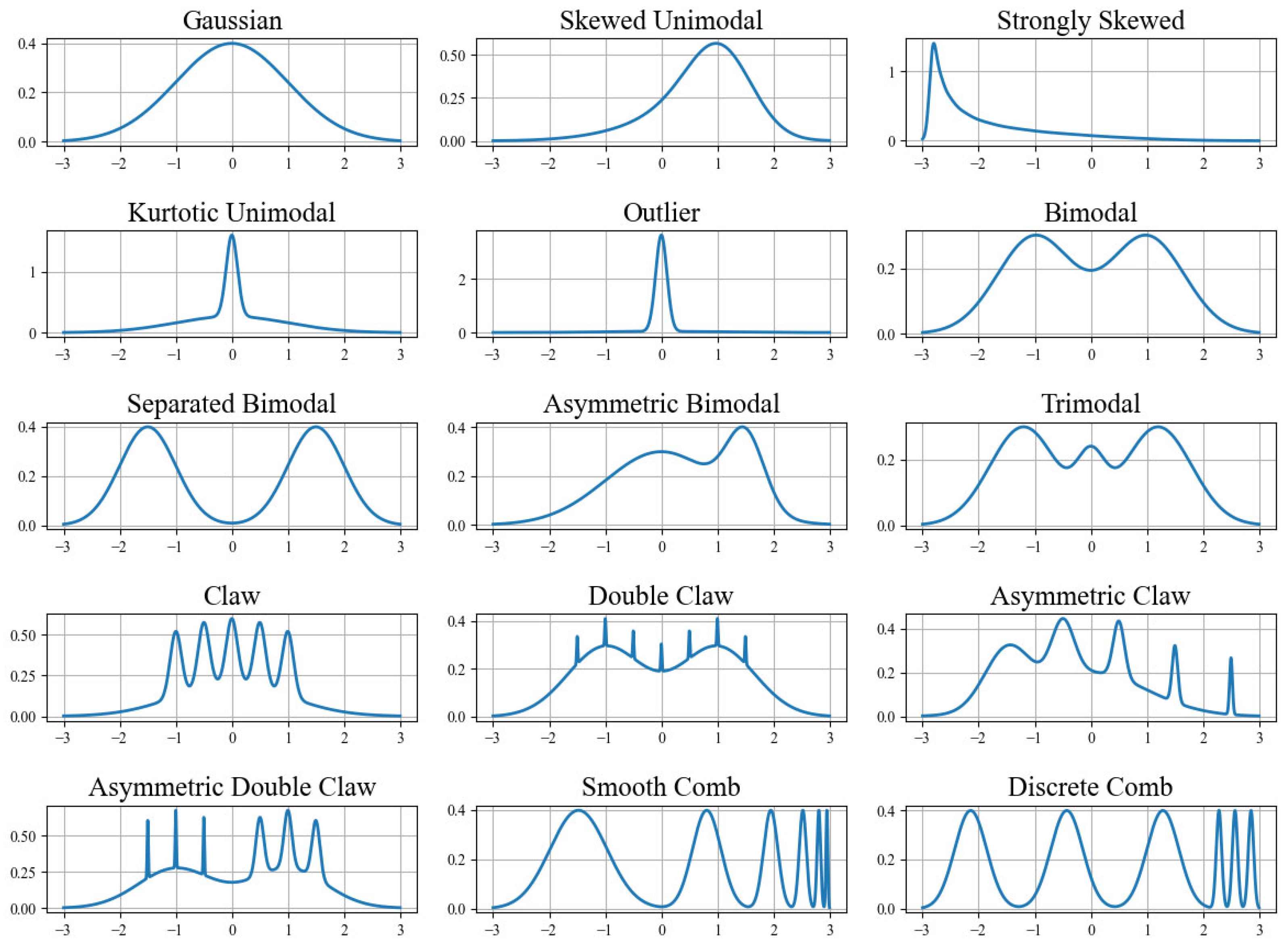
A comprehensive simulation study was conducted to compare the statistical estimation methods described previously. To avoid subjectivity in the comparative analysis, Gaussian mixture densities were used as target distributions. These mixtures were originally proposed by J.S. Marron and M.P. Wand [2] and include the following (also see Figure 1):

• Gaussian—$\mathcal{N}\left(0, 1\right)$
• Skewed Unimodal—${\displaystyle \frac{1}{5}}\mathcal{N}\left(\mathrm{0,1}\right)+{\displaystyle \frac{1}{5}}\mathcal{N}\left({\displaystyle \frac{1}{2}},{\left({\displaystyle \frac{2}{3}}\right)}^2\right)+{\displaystyle \frac{3}{5}}\mathcal{N}\left({\displaystyle \frac{13}{12}},{\left({\displaystyle \frac{5}{9}}\right)}^2\right)$
• Strongly Skewed—${\sum }_{l=0}^7{\displaystyle \frac{1}{8}}\mathcal{N}\left(3\left\{{\left({\displaystyle \frac{2}{3}}\right)}^l-1\right\},{\left({\displaystyle \frac{2}{3}}\right)}^{2l}\right)$
• Kurtotic Unimodal—${\displaystyle \frac{2}{3}}\mathcal{N}\left(\mathrm{0,1}\right)+{\displaystyle \frac{1}{3}}\mathcal{N}\left(0,{\left({\displaystyle \frac{1}{10}}\right)}^2\right)$
• Outlier—${\displaystyle \frac{1}{10}}\mathcal{N}\left(\mathrm{0,1}\right)+{\displaystyle \frac{9}{10}}\mathcal{N}\left(0,{\left({\displaystyle \frac{1}{10}}\right)}^2\right)$
• Bimodal—${\displaystyle \frac{1}{2}}\mathcal{N}\left(-1,{\left({\displaystyle \frac{2}{3}}\right)}^2\right)+{\displaystyle \frac{1}{2}}\mathcal{N}\left(1,{\left({\displaystyle \frac{2}{3}}\right)}^2\right)$
• Separated Bimodal—${\displaystyle \frac{1}{2}}\mathcal{N}\left(-{\displaystyle \frac{3}{2}},{\left({\displaystyle \frac{1}{2}}\right)}^2\right)+{\displaystyle \frac{1}{2}}\mathcal{N}\left({\displaystyle \frac{3}{2}},{\left({\displaystyle \frac{1}{2}}\right)}^2\right)$
• Asymmetric Bimodal—${\displaystyle \frac{3}{4}}\mathcal{N}\left(\mathrm{0,1}\right)+{\displaystyle \frac{1}{4}}\mathcal{N}\left({\displaystyle \frac{3}{2}},{\left({\displaystyle \frac{1}{3}}\right)}^2\right)$
• Trimodal—${\displaystyle \frac{9}{20}}\mathcal{N}\left(-{\displaystyle \frac{6}{5}},{\left({\displaystyle \frac{3}{5}}\right)}^2\right)+{\displaystyle \frac{9}{20}}\mathcal{N}\left({\displaystyle \frac{6}{5}},{\left({\displaystyle \frac{3}{5}}\right)}^2\right)+{\displaystyle \frac{1}{10}}\mathcal{N}\left(0,{\left({\displaystyle \frac{1}{4}}\right)}^2\right)$
• Claw—${\displaystyle \frac{1}{2}}\mathcal{N}\left(\mathrm{0,1}\right)+{\sum }_{l=0}^4{\displaystyle \frac{1}{10}}\mathcal{N}\left({\displaystyle \frac{l}{2}}-1,{\left({\displaystyle \frac{1}{10}}\right)}^2\right)$
• Double Claw—${\displaystyle \frac{49}{100}}\mathcal{N}\left(-1,{\left({\displaystyle \frac{2}{3}}\right)}^2\right)+{\displaystyle \frac{49}{100}}\mathcal{N}\left(1,{\left({\displaystyle \frac{2}{3}}\right)}^2\right)+{\sum }_{l=0}^6{\displaystyle \frac{1}{350}}\mathcal{N}\left({\displaystyle \frac{l-3}{2}},{\left({\displaystyle \frac{1}{100}}\right)}^2\right)$
• Asymmetric Claw—${\displaystyle \frac{1}{2}}\mathcal{N}\left(\mathrm{0,1}\right)+{\sum }_{l=-2}^2{\displaystyle \frac{2^{1-l}}{31}}\mathcal{N}\left(l+{\displaystyle \frac{1}{2}},{\left({\displaystyle \frac{2^{-l}}{10}}\right)}^2\right)$
• Asymmetric Double Claw—${\sum }_{l=0}^1{\displaystyle \frac{46}{100}}\mathcal{N}\left(2l-1,{\left({\displaystyle \frac{2}{3}}\right)}^2\right)+{\sum }_{l=1}^3{\displaystyle \frac{1}{100}}\mathcal{N}\left(-{\displaystyle \frac{l}{2}},{\left({\displaystyle \frac{1}{100}}\right)}^2\right)+{\sum }_{l=1}^3{\displaystyle \frac{7}{100}}\mathcal{N}\left({\displaystyle \frac{l}{2}},{\left({\displaystyle \frac{7}{100}}\right)}^2\right)$
• Smooth Comb—${\sum }_{l=0}^5{\displaystyle \frac{2^{5-l}}{63}}\mathcal{N}\left({\displaystyle \frac{\left(65-96{\left(\frac{1}{2}\right)}^2\right)}{21}},{\displaystyle \frac{{\left(\frac{32}{63}\right)}^2}{2^{2l}}}\right)$
• Discrete Comb—${\sum }_{l=0}^2{\displaystyle \frac{2}{7}}\mathcal{N}\left({\displaystyle \frac{12l-15}{7}},{\left({\displaystyle \frac{2}{7}}\right)}^2\right)+{\sum }_{l=8}^{10}{\displaystyle \frac{1}{21}}\mathcal{N}\left({\displaystyle \frac{2l}{7}},{\left({\displaystyle \frac{1}{21}}\right)}^2\right)$

The simulation was performed using small and medium sample sizes: 50, 100, 200, 400, 800, 1600, and 3200. For each case, 100,000 replications were generated. The number of Monte Carlo replications (100,000) was selected based on stability analysis. When using 10,000 replications, average error values were similar but confidence intervals were wider, leading to less clear method rankings. The higher replication count ensured stable estimates and tighter intervals for comparison.

To evaluate the accuracy of the density estimators, the following error measures were calculated:

$$MAE={\displaystyle \frac{1}{n}}\sum _{t=1}^n\left|f\left(X\left(t\right)\right)-\widehat{f}\left(X\left(t\right)\right)\right|\cong \int \left|f\left(x\right)-\widehat{f}\left(x\right)\right|f\left(x\right)dx$$

and

$$MAPE={\displaystyle \frac{1}{n}}\sum _{t=1}^n\left|{\displaystyle \frac{f\left(X\left(t\right)\right)-\widehat{f}\left(X\left(t\right)\right)}{f\left(X\left(t\right)\right)}}\right|\cong \int \left|f\left(x\right)-\widehat{f}\left(x\right)\right|dx.$$

In the next stage, decision-making algorithms were compared in terms of their ability to identify the most accurate density estimator for a given unknown distribution. The predictor vectors used by these algorithms included numerical features characterizing the data distribution, such as sample size, the skewness in absolute size, kurtosis, outliers, relative size of the sample, estimated number of clusters, and individual components of the clustered sample outlier ratio.

To estimate outliers in clustered samples, a rule-of-thumb known as the 3-sigma rule was applied. The results of the decision-making method comparison are presented in

Table 1. Misclassification rates for decision-making methods.

Methods	Training Set		Validation Set
	MAE	MAPE	MAE	MAPE
GLR	0.28081632	0.36843537	0.28476190	0.37142857
LDA	0.54897959	0.59959183	0.54730158	0.59650793
KDA	0.07659863	0.11455782	0.20825396	0.26761904
NN	0.19306122	0.25741497	0.27936508	0.33904762
GLR + NN	0.15986395	0.17795918	0.26888889	0.33015873
KDA + NN	0.12707483	0.17401361	0.19619048	0.27682540

Bold values indicate the method with the lowest error for each metric and set.

, originating from statistical process control [52]. Outliers were identified in each cluster of the GMM using the EM algorithm by the condition $\left\{X:\left|X-{\widehat{\mu }}_i\right|>z_{1-\alpha /2}{\widehat{\sigma }}_i, i=1,\dots ,q\right\}$, where $z$ is the quantile of the standard normal distribution and $\alpha =0.05$ denotes the confidence level [53].

Validation analysis was performed to evaluate the effectiveness of the decision-making systems. All samples from the Gaussian mixture models were split into two non-overlapping subsets—a training set and a validation set—using stratified simple random sampling with equal probability selection and without replacement [54].

The comparison error rate was defined as the proportion of incorrectly selected density estimators across all validation samples. The ratio between the training and validation sets was set at $7:3$, allowing the decision-making systems to be sufficiently trained while minimizing the overall comparison error rate.

3. Results

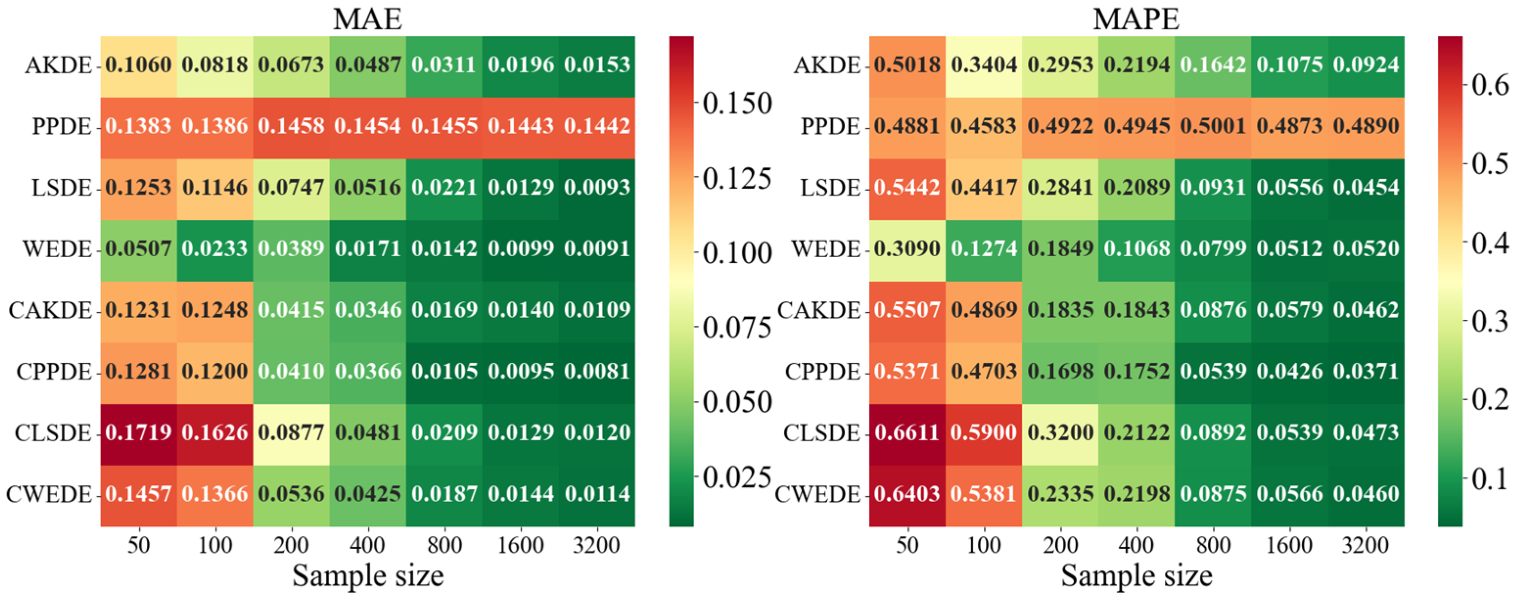
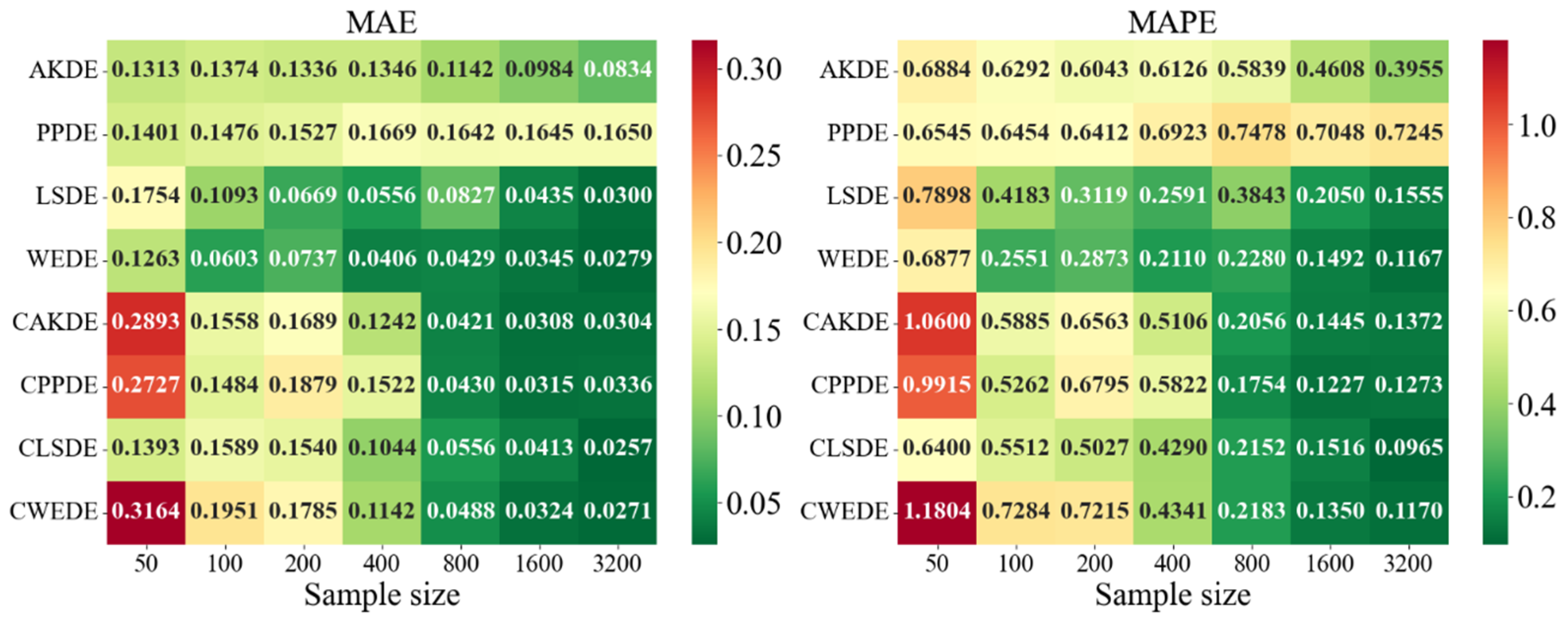
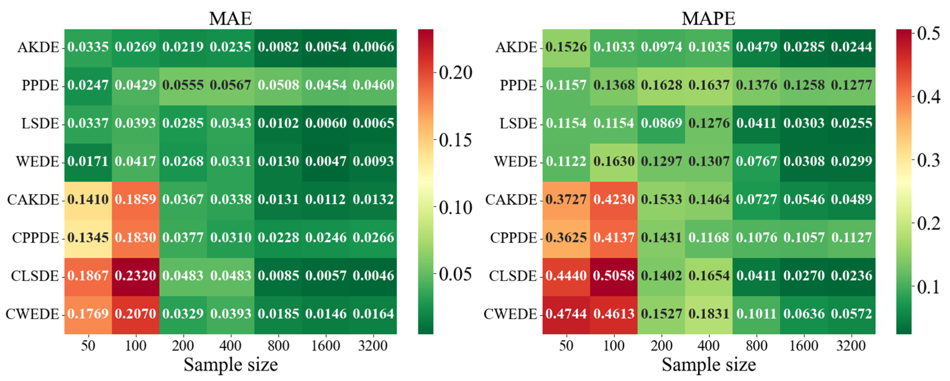
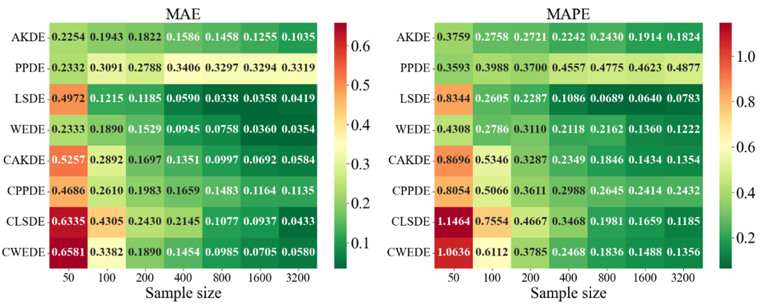
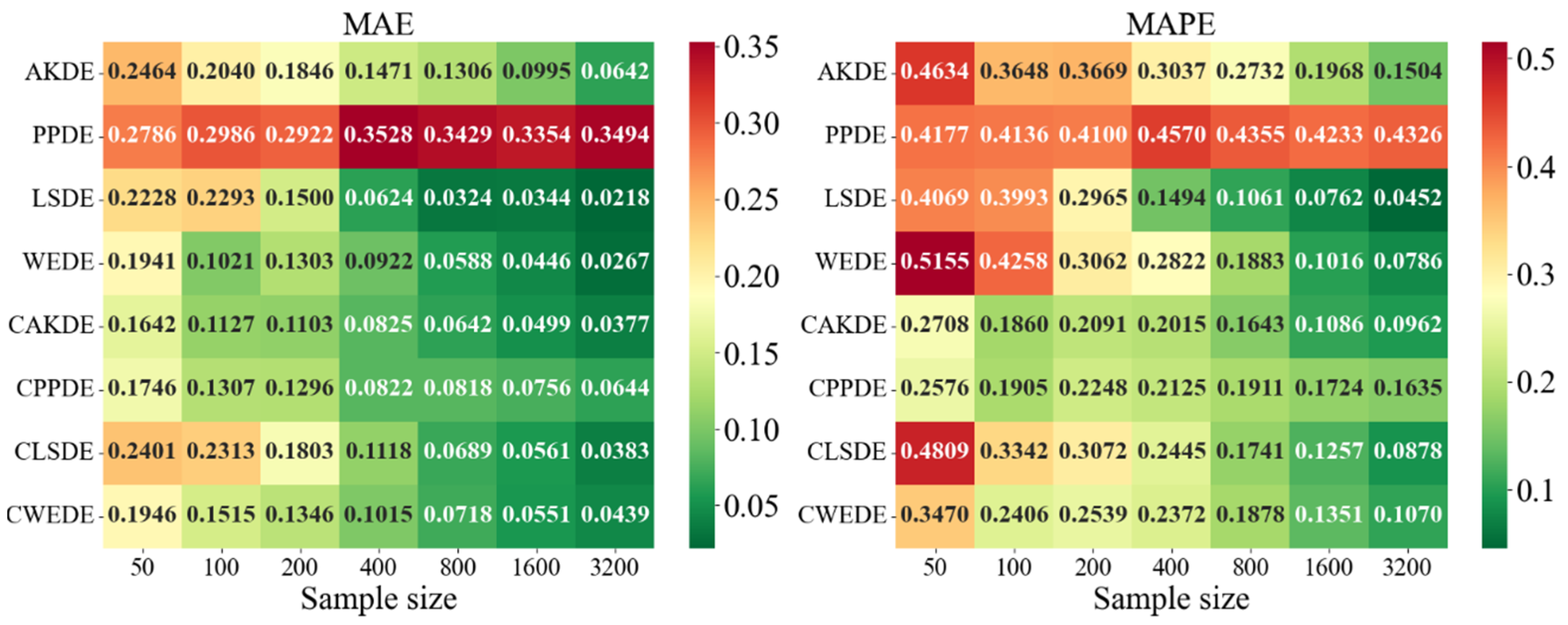
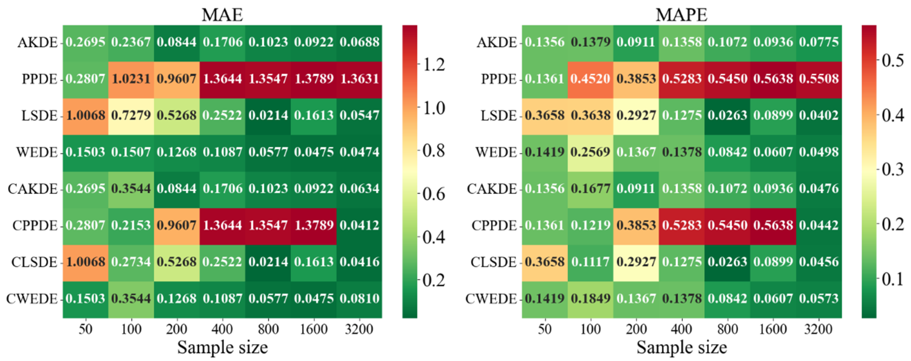
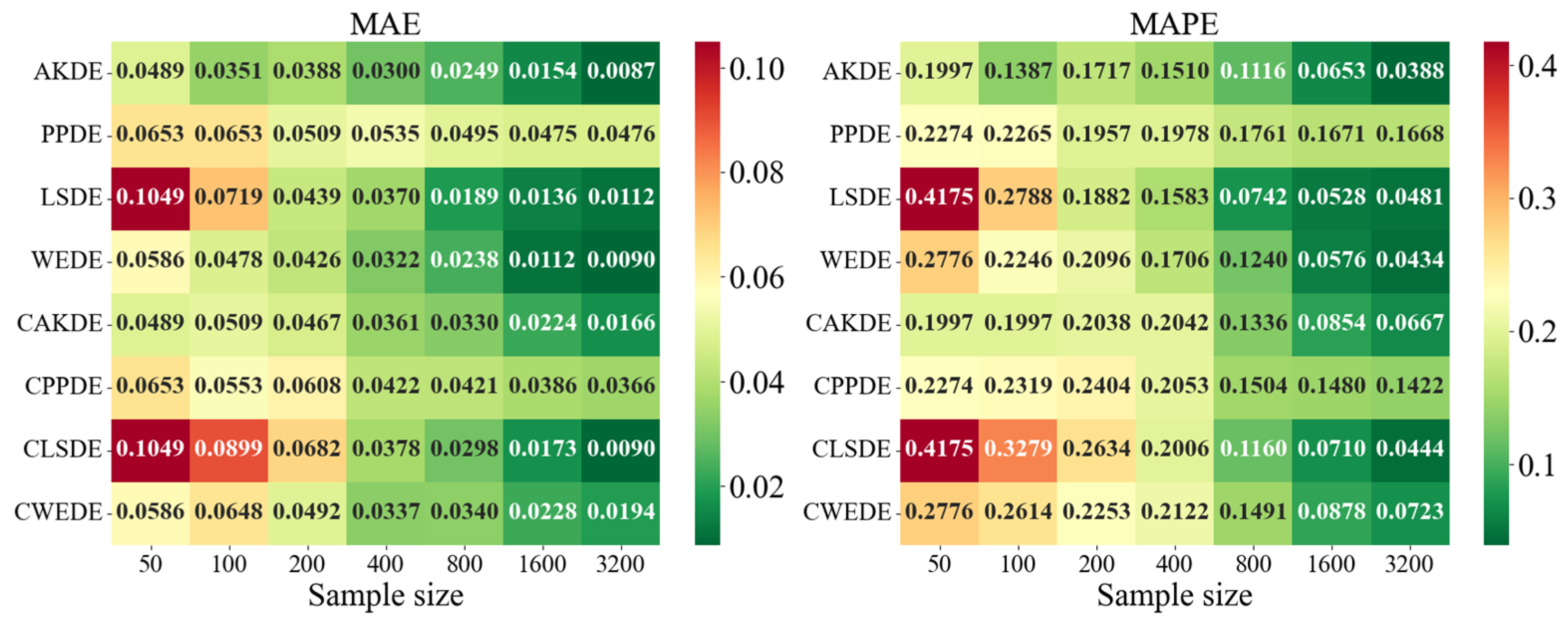
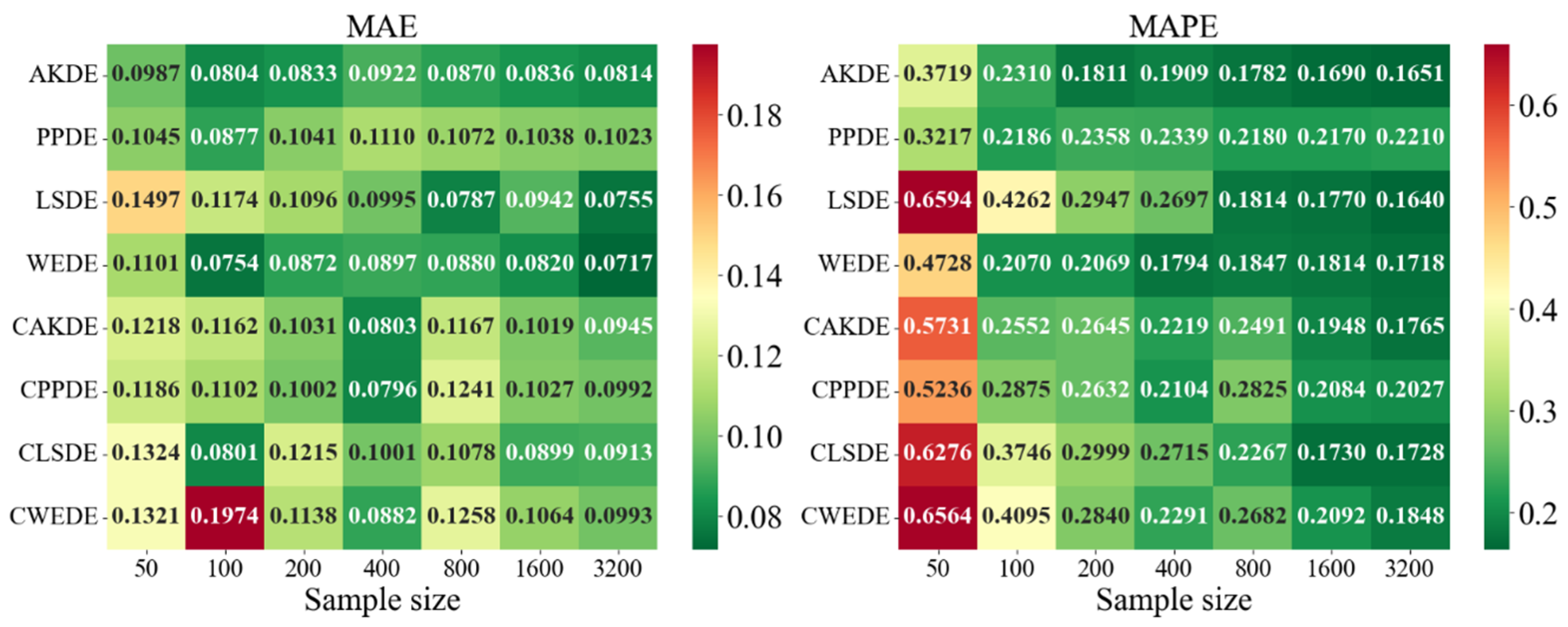
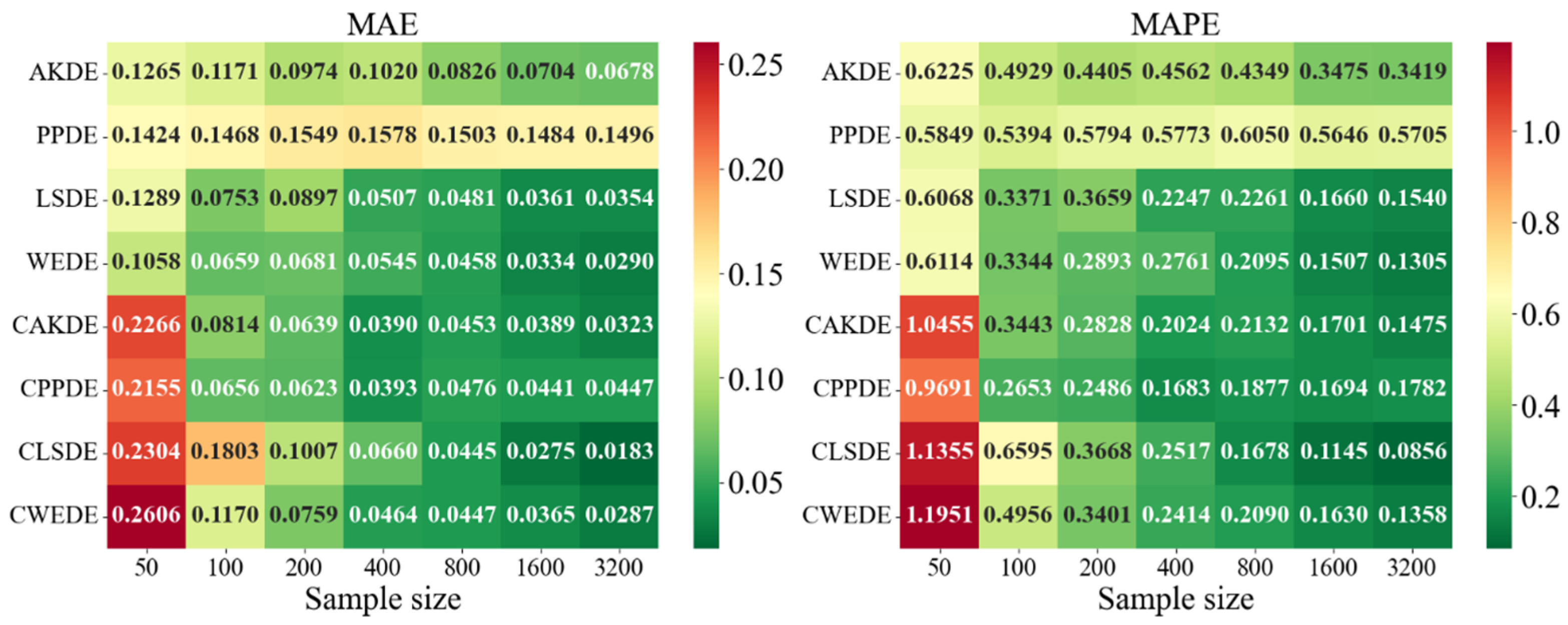
The error values for the applied methods, using optimally selected parameter values, are presented in Appendix A. These represent typical model cases; in other cases, the behavior of the errors was similar. For each method, the mean error values over $100$,$000$ samples are reported. Appendix A also provides graphical representations (heatmaps) of the density estimation results for the AKDE, PPDE, LSDE, and WEDE methods, both without and with initial data clustering. The latter results are denoted by a prefix C in front of the method name.

The general analysis showed that all methods exhibited a decreasing trend in MAE and MAPE values as sample size increased, confirming the consistency of the estimators. However, the precision gain differed depending on the method and the shape of the modeled density. While AKDE typically demonstrated stable performance, PPDE often showed better accuracy, especially for symmetric and multimodal densities. LSDE revealed its strength in larger samples, whereas WEDE frequently performed well when sensitivity to boundary values or local structure recovery was important.

The results of the decision-making method comparison are presented in Table 1. Here, the dependent variable is the method that most accurately estimated the density for each sample, based on both MAE and MAPE. GLR denotes generalized logistic regression, LDA—linear discriminant analysis, KDA—kernel discriminant analysis with Gaussian kernel (other kernels mentioned in Section 2.3 were also tested but yielded lower accuracy), and NN—a three-layer feedforward neural network with $20$ neurons. Additionally, hybrid approaches were used: a second neural network refined the results of the first method using the classification probabilities from the statistical method.

As shown in the table, KDA yielded the lowest error when decision-making methods were applied independently. Combining different methods improved accuracy in most cases compared to using them individually, with the exception of MAPE-based classification when applying KDA alone. Hybrid approaches led to $5.5\%$ to $11\%$ reductions in misclassification rates.

4. Discussion

The following discussion aims to contextualize the comparative results obtained from the simulation study. By examining the behavior of the four density estimation methods under varying distributional forms, we aim to evaluate their robustness, flexibility, and sensitivity to sample size, skewness, multimodality, and outliers. Special attention is given to the added value of clustering as a preprocessing step. An extended set of visual results supporting this discussion is provided in Figure A1, Figure A2, Figure A3, Figure A4, Figure A5, Figure A6, Figure A7, Figure A8, Figure A9, Figure A10, Figure A11, Figure A12, Figure A13, Figure A14 and Figure A15 in the Appendix A.

Focusing on specific results, in the case of the Gaussian density, all methods demonstrated good convergence. PPDE and LSDE were particularly notable, with their MAE values decreasing from $\approx 0.025-0.08$ (for $n=50$) to $\approx 0.004-0.006$ (for $n=3200$). This confirms their effectiveness when the target distribution is unimodal and close to normal. Although WEDE maintained stability, it slightly lagged behind in terms of precision.

For skewed unimodal distributions, performance differences became more evident. PPDE errors increased, especially for medium-sized samples, indicating sensitivity to skewness. In contrast, WEDE and LSDE adapted better to such structures, and clustering further improved their performance. This suggests that for distributions with substantial asymmetry, more flexible methods—particularly wavelet-based—yield higher accuracy.

Differences between methods were even more pronounced for strongly skewed densities. MAPE values sometimes exceeded $0.8$, especially for LSDE and CWEDE in small samples. However, as sample size increased, accuracy significantly improved, with WEDE consistently reducing error, even for such challenging distributions. Clustering played a critical role here—methods such as CAKDE and CWEDE were substantially more accurate than their non-clustered counterparts.

For complex multimodal distributions such as Bimodal, Trimodal, Claw, and Double Claw, WEDE and LSDE demonstrated notable strengths. WEDE effectively recovered fine modal structures, particularly for $n\ge 800$, while LSDE showed low MAE values in large samples. Nevertheless, without clustering, these methods were often ineffective in distinguishing mixture components. Clustered variants—especially CLSDE and CWEDE—performed significantly better by allowing each mode to be modeled individually, which is essential in multimodal scenarios.

In outlier-prone distributions, many methods struggled. PPDE and LSDE performed poorly without clustering, with MAPE often exceeding $0.5$ and, in some cases, surpassing 1. WEDE, however, retained high accuracy, highlighting its robustness to anomalies. Similarly, CAKDE and CWEDE were stable and significantly reduced errors, confirming the necessity of clustering for distributions with outlying features.

For asymmetric and complex densities (e.g., Asymmetric Bimodal, Asymmetric Claw, Asymmetric Double Claw), none of the methods were consistently stable across all sample sizes. Still, WEDE and LSDE (especially with clustering) showed consistent accuracy improvements as the sample size increased, with acceptable MAPE values achieved only from $n\approx 1600$. This suggests that for complex structures, effectiveness strongly depends on proper initial clustering and sufficiently large sample sizes.

In the last group of results—Comb-type densities characterized by highly intricate shapes and multiple localized peaks—WEDE demonstrated the highest stability, particularly for $n\ge 800$. LSDE showed impressive precision, but only in very large samples. Clustered methods, especially CLSDE and CWEDE, again significantly enhanced accuracy, confirming their versatility.

In summary, applying clustering generally improved the performance of all four methods. Although the improvement was not always dramatic, for densities with multiple modes or asymmetry, EM-based clustering proved to be a crucial step toward more accurately reconstructing the true density structure. It was also observed that some methods (especially PPDE) are highly sensitive to overlapping components and large variances, so their use without clustering should be approached with caution. While the accuracy of all methods improves with increasing sample size, the choice between them should be guided by the characteristics of the target density. For small samples, WEDE or CAKDE are recommended; for medium sizes, clustered versions of PPDE or LSDE are more suitable; and, for large samples, CLSDE, CWEDE, or even PPDE in its classical form may be effective. This confirms that no single method is universally optimal—the data nature and density structure must be considered to make a justified choice of the estimation method.

5. Conclusions

This study presented a comprehensive comparative analysis of four nonparametric density estimation methods—adaptive kernel density estimation (AKDE), projection pursuit density estimation (PPDE), log-spline density estimation (LSDE), and wavelet-based density estimation (WEDE)—applied to a wide range of univariate Gaussian mixture distributions. The analysis covered both classical methods and their extended versions, which included data clustering using the EM algorithm. Estimation accuracy was assessed using MAE and MAPE criteria across various sample sizes, allowing for an in-depth evaluation of method behavior and stability.

The results revealed that no single estimation method consistently outperformed the others across all density types and sample sizes. In small samples, simpler methods such as AKDE or PPDE yielded lower errors for symmetric and low-modality densities, but their performance deteriorated significantly when faced with asymmetry or fragmented structures. In contrast, LSDE and WEDE showed greater flexibility and the ability to reconstruct localized features, particularly in larger samples. Wavelet-based estimators were especially effective for densities with sharp transitions or localized extrema.

One of the key contributions of this work was the analysis of clustering as a preprocessing step. Clustered versions of the methods consistently outperformed their unclustered counterparts for multimodal, asymmetric, and outlier-prone distributions. Clustering the sample using the EM algorithm allowed each component to be modeled separately, reducing overall estimation error. This was particularly valuable for distributions with overlapping or distant components (e.g., “Separated Bimodal”, “Asymmetric Claw”, “Outlier”). These results underscore the importance of incorporating clustering into the analytical pipeline for more complex distributions.

Additionally, the effectiveness of decision-making systems (GLM, LDA, KDA, and MLP-type neural networks) was evaluated for automatically selecting the most appropriate density estimation method based on sample characteristics such as skewness, kurtosis, modality, outlier frequency, number of clusters, etc. Validation showed that the neural network-based system (MLP) had the lowest rate of incorrect method selection—on average, $18.4\%$—whereas simpler models such as GLM or LDA ranged between $24\%$ and $31\%$. This indicates that even in analytically complex scenarios, neural networks can effectively automate the method selection process, reducing the influence of subjectivity.

Overall, the findings suggest that effective nonparametric density estimation requires a combined approach—first analyzing the structure of the sample (e.g., through clustering) and then applying intelligent decision-making algorithms. The existence of a universally optimal method is unlikely; however, by systematically applying model selection principles, high levels of generalizability can be achieved.

Future research should extend this work to the multivariate case, where both clustering and estimation become more complex. It is also relevant to investigate dynamically adaptive decision-making systems capable of operating in real-time data stream environments. Further attention should be given to applying deep neural networks to the estimator selection problem, incorporating automated feature engineering and ensemble methods. Finally, practical applications in real-world domains such as anomaly detection, signal processing, and financial modeling could become an important direction for further investigation.