Statistical Analysis of a Generalized Linear Model for Bilateral Correlated Data Under Donner’s Model

Abstract

Paired data often arise in medical studies, with a correlation between responses of paired organs or parts. Under an intra-correlated model, this paper proposes a generalized linear model to investigate probable confounding factors of the individual response rates in paired data. The main link functions include logistic, log–log, complementary log–log, probit, and double exponential. The estimators of model parameters are calculated through the Newton–Raphson, quadratic lower bound, and Fisher bounded algorithms. Then, three tests (i.e., likelihood ratio test, Wald-type test, and score test) are constructed to analyze whether covariates significantly affect the response rate. Finally, the proposed methods are illustrated by numerical simulation and visual impairment data from Iran.

1. Introduction

In medical studies, paired data (i.e., eyes, ears, and arms) are often encountered from paired organs or parts of patients. For each individual, the outcomes for paired organs may be neither, only one, or both responses. A specific correlation is usually considered to avoid biased results. Until now, various intra-correlated models have been proposed to investigate dependent properties, such as Ronser’s model [1], Dallal’s model [2], and Donner’s model [3]. The first two models reflect response dependence through conditional probabilities, which may be inapplicable in some extreme cases, while Donner’s model is based on a correlation coefficient $\rho$. Thompson [4] considered that Donner’s model is more effective than others. Significant progress has been made in the study of response rates under these intra-correlated models [5,6,7,8,9,10]. However, existing research primarily focuses on whether confounding factors significantly impact response rate risk measures. For example, Zhang and Ma [11] analyzed the homogeneity of differences between two proportions for stratified data across strata. Hua and Ma [12] assessed the significance of treatment effects on the ratio of response rates. Sun et al. [13] proposed three testing methods to evaluate the homogeneity of the risk difference in stratified data. These results cannot provide the effect of various factors on response rates.

The generalized linear model is an extension of the traditional linear regression model, designed to accommodate a broader range of data types and distributions [14,15,16]. Logistic regression is widely used to investigate binary data [17,18]. The classical logistic regression model assumes that the observations are independent. Taking into account the correlated data [19,20,21,22], Lin et al. [23] constructed a logistic regression model to explore the relationship between the incidence of ophthalmic disease and the covariates under Donner’s model. However, the dependency curve between the response rate and confounding effects is often unknown. Although logistic regression can solve such correlated data, it may result in inadequate model fitting in the context of complex relationships, failing to fully capture the nonlinear associations between these variables. Based on the preceding analysis, the innovations of the article are summarized below:

(i)

A generalized linear model with correlated data is proposed to investigate the relationship between the response rate and confounding effects, so the logistic model is a special case [23].

(ii)

The Newton–Raphson (NR) iterative algorithm calculates maximum likelihood estimators (MLEs) of unknown parameters. Considering the complexity of the link function, the quadratic lower bound (QLB) and the Fisher bounded algorithm are further introduced.

(iii)

The likelihood ratio test, Wald-type test, and score test are constructed to analyze whether the confounding effects significantly impacted the response rate.

(iv)

Numerical simulations compare the performance of algorithms and statistics. Real data is studied to illustrate the proposed methods.

The rest of the paper is organized as follows. In Section 2, we first introduce the generalized linear model and the log-likelihood under the Donner framework. Then, three iterative algorithms for parameter estimation and hypothesis testing are conducted. The main results are provided in Section 3, and an application is used to illustrate the theoretical results in Section 4. Section 5 gives the discussion and a brief conclusion.

2. Methods

2.1. Generalized Linear Model with Correlated Data

When each individual in the study contributes the measurements of paired organs, the overall outcome may be neither, only one, or both responses; this is called bilateral data. If a certain correlation exists between paired organs’ responses, it is called bilateral correlated data. Let $Z_{ik}=1$ if the k-th organ of the i-th individual has a response, and $Z_{ik}=0$ otherwise for $k=1,2$, $i=1,\dots ,n$. Suppose that $Z_{ik}$ are independent and Bernoulli-distributed with probabilities ${\pi }_i$, that is, $Z_{ik}\sim Bernoulli(1,{\pi }_i)$. Thus, $E\left[Z_{ik}\right]=P(Z_{ik}=1)={\pi }_i(i=1,\dots ,n)$. Under Donner’s model, we have $\mathrm{Corr}(Z_{ik},Z_{i(3-k)})=\rho$ for $k=1,2$, and $i=1,\dots ,n$, where $\rho \left(\right|\rho |\le 1)$ reflects the correlation of the paired data. Denote by $p_{li}$ the corresponding probability of $l=(0,1,2)$ response(s) of the i-th individual. By calculation, the probabilities of neither, one, or both responses can be obtained by

$$p_{0i}=\rho (1-{\pi }_i)+(1-\rho ){(1-{\pi }_i)}^2,p_{1i}=2{\pi }_i(1-\rho )(1-{\pi }_i),p_{2i}=\rho {\pi }_i+(1-\rho ){\pi }_i^2,$$

for $i=1,2,\dots ,n$, satisfying $0\le p_{li}\le 1$, and ${\sum }_{l=0}^2{p}_{li}=1$. The detailed calculations are provided in the Appendix A.1. Let $Y_i$ be the response variable of paired organs of the ith individual, and take the values 0, 1, 2, where $Y_i=0$ indicates that neither of the two organs has the response, $Y_i=1$ indicates that only one organ has the response, and $Y_i=2$ indicates that both organs have the responses. Denote $\mathit{\pi }=({\pi }_1,\dots ,{\pi }_n)$. Based on the probabilities $p_{li}(l=0,1,2),$ we obtain the likelihood function

$$\begin{array}{cc}\hfill L(\mathit{\pi },\rho )& =\prod _{i=1}^n{p}_{0i}^{I(Y_i=0)}{p}_{1i}^{I(Y_i=1)}{p}_{2i}^{I(Y_i=2)},\hfill \end{array}$$

where $I(·)$ denotes the indicator function. Take the natural logarithm of both sides of $L(\mathit{\pi },\rho )$, thereby obtaining the log-likelihood function:

$$\begin{array}{cc}\hfill \ell (\mathit{\pi },\rho )& =\sum _{i=1}^n\{I(Y_i=0)log\left[(1-{\pi }_i)(\rho {\pi }_i-{\pi }_i+1)\right]+I(Y_i=1)log\left[2{\pi }_i(1-\rho )(1-{\pi }_i)\right]\hfill \\ \hfill & +I(Y_i=2)log[{\pi }_i^2+\rho {\pi }_i(1-{\pi }_i)]\}.\hfill \end{array}$$

(1)

To investigate the relationship between response rates of n different individuals and confounding factors (e.g., age), we introduce a generalized linear model (GLM) as follows:

$$g\left({\pi }_i\right)={\mathbf{x}}_i^T\mathit{\beta },i=1,\dots ,n,$$

(2)

where ${\mathbf{x}}_i={(1,x_{i\left(1\right)},\dots ,x_{i(q-1)})}^T$ is the covariate vector of interest, $\mathit{\beta }={({\beta }_0,{\beta }_1,\dots ,{\beta }_{q-1})}^T$ is the vector of unknown regression coefficients, and $g(·)$ is a monotonic and differentiable link function. In this work, we mainly use the following link functions:

(i)

Logistic link function. The logistic link function is typically used in the model (2) to analyze the relationship between a binary response variable and linear predictor variables. Take the link function $g\left({\pi }_i\right)=ln({\pi }_i/(1-{\pi }_i))$.

(ii)

Log–log and complementary log–log. When the response probability exhibits asymmetry or there is a high likelihood of extreme events, the log–log or complementary log–log link function can better capture the characteristics of the data. The log–log link function $g\left({\pi }_i\right)=log(-log(1-{\pi }_i))$, and the complementary log–log link function $g\left({\pi }_i\right)=log(-log\left({\pi }_i\right))$.

(iii)

Power family. Considering that the response rate falls within the $(0,1)$ range, a power family distribution with a shape parameter is appropriate as a link function [24]. Its distribution is indexed by shape parameters as follows:

$$F_p\left(x\right)={\displaystyle \frac{p{\omega }_p^{1/2p}}{\mathrm{\Gamma }(1/2p)}}{\int }_{-\infty }^x{e}^{-{\omega }_p{\left|t\right|}^{2p}}dt,$$

where p is the shape parameter, ${\omega }_p=1/2p$, and $\mathrm{\Gamma }(·)$ is the gamma function. Specifically, the power family derives two link functions: the double exponential (DE) link function ${\pi }_i={\displaystyle \frac{1}{2}}{\int }_{-\infty }^{{\mathbf{x}}_i^T\beta }{e}^{-\left|t\right|}dt$ and the probit (Pt) link function $g\left({\pi }_i\right)={\mathrm{\Phi }}^{-1}\left({\pi }_i\right)$, which correspond to $p=1/2$ and $p=1$, respectively. As the distribution is symmetric, it can be used as a symmetric link function to describe symmetric response characteristics.

Table 1. Comparison of five link functions.

Link Function	${\mathit{\pi }}_{\mathit{i}}$	Applicable Data	Advantages	Algorithm
Logistic (L)	${\pi }_i={\displaystyle \frac{e^{{\mathbf{x}}_i^T\mathit{\beta }}}{1+e^{{\pi }_i^T\mathit{\beta }}}}$	Symmetric response probabilities	Interpretable, widely used	QLB-NR
Log–log (LL)	${\pi }_i=1-e^{-e^{{\mathbf{x}}_i^T\mathit{\beta }}}$	Right-extreme (near 0 to increasing)	Asymmetric right-skewed data	FB-NR
Complementary log–log (CLL)	${\pi }_i=e^{-e^{{\mathbf{x}}_i^T\mathit{\beta }}}$	Left-extreme (near 1 to decreasing)	Asymmetric left-skewed data	FB-NR
Double exponential (DE)	${\pi }_i={\displaystyle \frac{1}{2}}{\int }_{-\infty }^{{\mathbf{x}}_i^T\mathit{\beta }}{e}^{-\left|t\right|}dt$	Symmetric, extreme events	Strong symmetry	FB-NR
Probit (Pt)	${\pi }_i=\mathrm{\Phi }\left({\mathbf{x}}_i^T\mathit{\beta }\right)$	Symmetric, near-normal	High accuracy, low errors	FB-NR

Note. QLB-NR: Quadratic lower-bound-based NR algorithm; FB-NR: Fisher-bound-based NR algorithm.

provides a summary of the five link functions.

Denote $h\left({\mathbf{x}}_i^T\mathit{\beta }\right)={\pi }_i=g^{-1}\left({\mathbf{x}}_i^T\mathit{\beta }\right)$; the function (1) can be rewritten as

$$\begin{array}{cc}\hfill \ell (\mathit{\beta },\rho )=& \sum _{i=1}^n\{I(Y_i=0)log\left[(1-h\left({\mathbf{x}}_i^T\mathit{\beta }\right))(\rho h\left({\mathbf{x}}_i^T\mathit{\beta }\right)-h\left({\mathbf{x}}_i^T\mathit{\beta }\right)+1)\right]\hfill \\ \hfill & +I(Y_i=1)log\left[2h\left({\mathbf{x}}_i^T\mathit{\beta }\right)(1-\rho )(1-h\left({\mathbf{x}}_i^T\mathit{\beta }\right))\right]\hfill \\ \hfill & +I(Y_i=2)log[h^2\left({\mathbf{x}}_i^T\mathit{\beta }\right)+\rho h\left({\mathbf{x}}_i^T\mathit{\beta }\right)(1-h\left({\mathbf{x}}_i^T\mathit{\beta }\right))]\}.\hfill \end{array}$$

(3)

Given the link function $g\left({\pi }_i\right)$, we can estimate the unknown coefficient vector $\mathit{\beta }$ and the correlation coefficient $\rho$. Some studies have demonstrated that maximum likelihood estimation (MLE) remains valid even when there is correlation between parameters [25]. By fixing one parameter and computing the partial derivative of the log-likelihood function (3) for the other parameter [26], we obtain easily computable derivatives to $\mathit{\beta }$ and $\rho$. Setting these derivatives to zero, that is, ${\displaystyle \frac{\partial \ell }{\partial \beta }}=0,{\displaystyle \frac{\partial \ell }{\partial \rho }}=0.$ Thus, the MLEs are the solution of the above equations. However, since closed-form solutions do not exist, specific algorithms must be proposed to address this issue. In the following section, we focus on these algorithms to estimate the values of unknown parameters for different link functions.

2.2. Parameter Estimation

Based on the link functions, the NR algorithm is first used to estimate the correlation coefficient $\rho$. For the regression coefficient vector $\mathit{\beta }$, the NR algorithm may fail to converge in certain situations, particularly for complex link functions. In such cases, the QLB algorithm is proposed for the logistic link function, while the Fisher-bounded algorithm is proposed for the remaining link functions.

Newton–Raphson algorithm. Given the t-th approximations ${\pi }^{\left(t\right)}$ and ${\rho }^{\left(t\right)}$, the $(t+1)$th approximation of the MLE $\widehat{\rho }$ can be calculated via the NR algorithm:

$${\rho }^{(t+1)}={\rho }^{\left(t\right)}-{\left[{\displaystyle \frac{{\partial }^2\ell ({\mathit{\pi }}^{\left(t\right)},{\rho }^{\left(t\right)})}{\partial {\rho }^2}}\right]}^{-1}{\displaystyle \frac{\partial \ell ({\mathit{\pi }}^{\left(t\right)},{\rho }^{\left(t\right)})}{\partial \rho }},$$

where

$$\begin{array}{cc}\hfill {\displaystyle \frac{\partial \ell (\mathit{\pi },\rho )}{\partial \rho }}=& \sum _{i=1}^n\left[{\displaystyle \frac{{\pi }_{i}I(Y_i=0)}{{\pi }_i(\rho -1)+1}}+{\displaystyle \frac{I(Y_i=1)}{\rho -1}}+{\displaystyle \frac{(1-{\pi }_i)I(Y_i=2)}{{\pi }_i+\rho (1-{\pi }_i)}}\right],\hfill \\ \hfill {\displaystyle \frac{{\partial }^2\ell (\mathit{\pi },\rho )}{\partial {\rho }^2}}=& -\sum _{i=1}^n\left[{\displaystyle \frac{{\pi }_i^{2}I(Y_i=0)}{{(\rho {\pi }_i-{\pi }_i+1)}^2}}+{\displaystyle \frac{I(Y_i=1)}{{(\rho -1)}^2}}+{\displaystyle \frac{{({\pi }_i-1)}^{2}I(Y_i=2)}{{(\rho +{\pi }_i-\rho {\pi }_i)}^2}}\right].\hfill \end{array}$$

Although the MLE of $\rho$ can be obtained, the parameter vector $\mathit{\beta }$ cannot be directly calculated by the NR algorithm. We use the assembly and decomposition (AD) approach proposed by [27] to construct a surrogate function $Q\left(\mathit{\pi }\right|{\mathit{\pi }}^{\left(t\right)},\rho )$ as follows:

$$Q\left(\mathit{\pi }\right|{\mathit{\pi }}^{\left(t\right)},\rho )=\sum _{i=1}^n\left\{a_i({\pi }_i^{\left(t\right)},\rho )log\left({\pi }_i\right)+b_i({\pi }_i^{\left(t\right)},\rho )log(1-{\pi }_i)+c_i^{\left(t\right)}\left(\rho \right)\right\},$$

where ${\pi }_i^{\left(t\right)}$ is the tth approximation of ${\pi }_i$, $c_i^{\left(t\right)}\left(\rho \right)$ is independent of ${\pi }_i(i=1,\dots ,n)$, and

$$\begin{array}{cc}\hfill a_i({\pi }_i^{\left(t\right)},\rho )& =I(Y_i=1)+I(Y_i=2)+{\displaystyle \frac{I(Y_i=2){\pi }_i^{\left(t\right)}}{{\pi }_i^{\left(t\right)}+\rho (1-{\pi }_i^{\left(t\right)})}}+{\displaystyle \frac{I(Y_i=0)\rho {\pi }_i^{\left(t\right)}}{\rho {\pi }_i^{\left(t\right)}+(1-{\pi }_i^{\left(t\right)})}},\hfill \\ \hfill b_i({\pi }_i^{\left(t\right)},\rho )& =I(Y_i=0)+I(Y_i=1)+{\displaystyle \frac{I(Y_i=2)\rho (1-{\pi }_i^{\left(t\right)})}{{\pi }_i^{\left(t\right)}+\rho (1-{\pi }_i^{\left(t\right)})}}+{\displaystyle \frac{I(Y_i=0)(1-{\pi }_i^{\left(t\right)})}{\rho {\pi }_i^{\left(t\right)}+(1-{\pi }_i^{\left(t\right)})}}.\hfill \end{array}$$

The detailed construction process is provided in Appendix A.2. The function $Q\left(\pi \right|{\pi }^{\left(t\right)},\rho )$ satisfies the condition $\ell \left(\mathit{\pi },\rho \right)-Q\left(\mathit{\pi }|{\mathit{\pi }}^{\left(t\right)},\rho \right)\ge 0.$ Replacing ${\pi }_i$ in the surrogate function with ${\pi }_i=h\left({\mathbf{x}}_i^T\mathit{\beta }\right)$, we have

$$Q\left(\mathit{\beta }\right|{\mathit{\beta }}^{\left(t\right)},\rho )=\sum _{i=1}^n\left\{a_i({\pi }_i^{\left(t\right)},\rho )log\left[h\left({\mathbf{x}}_i^T\mathit{\beta }\right)\right]+b_i({\pi }_i^{\left(t\right)},\rho )log[1-h\left({\mathbf{x}}_i^T\mathit{\beta }\right)]+c_i^{\left(t\right)}\left(\rho \right)\right\}.$$

Given $({\mathit{\beta }}^{\left(t\right)},{\rho }^{\left(t\right)})$, the $(t+1)$th approximation of the MLEs $\mathit{\beta }$ can be obtained by

$${\mathit{\beta }}^{(t+1)}=arg\underset{\mathit{\beta }\in {\mathbb{R}}^q}{max}Q(\mathit{\beta }\mid {\mathit{\beta }}^{\left(t\right)},{\rho }^{\left(t\right)}).$$

(4)

Thus, we can use the NR algorithm to calculate Equation (4) by

$$\begin{array}{c}\hfill {\mathit{\beta }}^{(t+1)}={\mathit{\beta }}^{\left(t\right)}-{\left[{\displaystyle \frac{{\partial }^{2}Q(\mathit{\beta }\mid {\mathit{\beta }}^{\left(t\right)},\rho )}{\partial \mathit{\beta }\partial {\mathit{\beta }}^{\prime }}}\right]}_{\mathit{\beta }={\mathit{\beta }}^{\left(t\right)}}^{-1}{\left[{\displaystyle \frac{\partial Q(\mathit{\beta }\mid {\mathit{\beta }}^{\left(t\right)},\rho )}{\partial \mathit{\beta }}}\right]}_{\mathit{\beta }={\mathit{\beta }}^{\left(t\right)}}.\end{array}$$

In practice, the NR algorithm may be unsuitable for all link functions since it may fail to guarantee the monotonic increase in the objective function $Q\left(\mathit{\beta }\right|{\mathit{\beta }}^{\left(t\right)},\rho )$ in each iteration. Based on this, we can adopt the QLB algorithm to estimate the MLEs.

Quadratic lower-bound-based NR algorithm. The QLB algorithm improves the NR algorithm using a parameter-independent quadratic lower-bound matrix, replacing the negative observed information matrix [28]. The key idea is to find a negative definite matrix B, independent of the unknown parameters, such that ${\displaystyle \frac{{\partial }^{2}Q\left({\beta }^{\left(t\right)}\right)}{\partial \beta \partial {\beta }^{\prime }}}\ge B$ for solving the extreme value problem (4) as follows:

$${\mathit{\beta }}^{(t+1)}={\mathit{\beta }}^{\left(t\right)}-B^{-1}\left({\displaystyle \frac{\partial Q\left({\mathit{\beta }}^{\left(t\right)}\right|{\mathit{\beta }}^{\left(t\right)},\rho )}{\partial \mathit{\beta }}}\right).$$

Thus, the algorithm avoids computing the inverse of the observed information matrix at each iteration to reach a maximum. Compared with other algorithms, such as the Broyden–Fletcher–Goldfarb–Shanno (BFGS) algorithm, the QLB may be computationally more straightforward and efficient. The detailed process of the QLB-based NR algorithm is given in Algorithm 1.

Algorithm 1: QLB-based NR algorithm

For the logistic link function, the MLEs of $\mathit{\beta }$ can be calculated:

$$\begin{array}{cc}\hfill Q{\left(\mathit{\beta }\right|{\mathit{\beta }}^{\left(t\right)},\rho )}_{logistic}& =\sum _{i=1}^n\left\{a_i({\pi }_i^{\left(t\right)},\rho ){\mathbf{x}}_i^T\mathit{\beta }-[a_i({\pi }_i^{\left(t\right)},\rho )+b_i({\pi }_i^{\left(t\right)},\rho )]log(1+e^{{\mathbf{x}}_i^T\mathit{\beta }})+c_i^{\left(t\right)}\left(\rho \right)\right\}.\hfill \end{array}$$

Then

$${\displaystyle \frac{\partial Q{\left(\mathit{\beta }\right|{\mathit{\beta }}^{\left(t\right)},{\rho }^{\left(t\right)})}_{logistic}}{\partial \mathit{\beta }}}{|}_{\mathit{\beta }={\mathit{\beta }}^{\left(t\right)}}=\sum _{i=1}^n\left\{[a_i({\pi }_i^{\left(t\right)},\rho )-2{\pi }_i^{\left(t\right)}]{\mathbf{x}}_i\right\}={\mathbf{X}}^{\mathrm{T}}\left[{\mathbf{y}}^{\left(t\right)}-2{\mathit{\pi }}^{\left(t\right)}\right],$$

where ${\mathbf{y}}^{\left(t\right)}={(a_1({\pi }_1^{\left(t\right)},{\rho }^{\left(t\right)}),\dots ,a_n({\pi }_n^{\left(t\right)},{\rho }^{\left(t\right)}))}^{\mathrm{T}},$ ${\mathbf{X}}_{n\times q}={(x_1,\dots ,x_n)}^{\mathrm{T}}$, and ${\mathit{\pi }}^{\left(t\right)}$ =$({\pi }_1^{\left(t\right)},$$\dots ,$${\pi }_n^{\left(t\right)}{)}^{\mathrm{T}}$. Moreover,

$${\displaystyle \frac{{\partial }^{2}Q{\left(\mathit{\beta }\right|{\mathit{\beta }}^{\left(t\right)},{\rho }^{\left(t\right)})}_{logistic}}{\partial \mathit{\beta }\partial {\mathit{\beta }}^{\prime }}}{|}_{\mathit{\beta }={\mathit{\beta }}^{\left(t\right)}}=\sum _{i=1}^n-\left\{2{\pi }_i^{\left(t\right)}(1-{\pi }_i^{\left(t\right)}){\mathbf{x}}_i{\mathbf{x}}_i^{\mathrm{T}}\right\}=-2{\mathbf{X}}^{\mathrm{T}}\mathbf{N}\mathbf{X},$$

where $N=\mathrm{diag}({\pi }_1^{\left(t\right)}(1-{\pi }_1^{\left(t\right)}),{\pi }_2^{\left(t\right)}(1-{\pi }_2^{\left(t\right)}),\dots ,{\pi }_n^{\left(t\right)}(1-{\pi }_n^{\left(t\right)})).$ For the inequality ${\pi }_i(1-{\pi }_i)\le 1/4(i=1,\dots ,n)$, the bound value of the logistic link function is 0.25. So, $B=-(1/2){\mathbf{X}}^{\mathrm{T}}\mathbf{X}$. Further, the MLEs of $\mathit{\beta }$ are calculated as follows:

$${\mathit{\beta }}^{(t+1)}={\mathit{\beta }}^{\left(t\right)}+2{\left({\mathbf{X}}^{\mathrm{T}}\mathbf{X}\right)}^{-1}{\mathbf{X}}^{\mathrm{T}}\left[{\mathbf{y}}^{\left(t\right)}-2{\pi }^{\left(t\right)}\right].$$

Note that the above iterative formula applies to low- and high-dimensional scenarios. Regularization techniques can be used to avoid overfitting and promote stability in high-dimensional cases. For other link functions, $a_i({\pi }_i^{\left(t\right)},\rho )$ and $b({\pi }_i^{\left(t\right)},\rho )$ are not constant, making ${\displaystyle \frac{{\partial }^{2}Q(\mathit{\beta }\mid {\mathit{\beta }}^{\left(t\right)},{\rho }^{\left(t\right)})}{\partial \mathit{\beta }\partial {\mathit{\beta }}^{\prime }}}$ variable and the lower bound matrix B hard to determine. Therefore, the Fisher-bound algorithm is proposed to estimate regression coefficients.

Fisher-bound-based NR algorithm. The Fisher scoring method is usually sensitive to initial values, and consequently, there may be difficulties in obtaining convergence. Under certain general conditions on the information matrix, the bounded algorithm [27] has been shown to consistently converge to the MLE, independent of the initial values. The specific iterative process of this algorithm is as follows:

$$\begin{array}{c}\hfill {\mathit{\beta }}^{(t+1)}={\mathit{\beta }}^{\left(t\right)}+B^{-1}{S}_c\left({\mathit{\beta }}^{\left(t\right)}\right).\end{array}$$

For a random variable $\eta \in (-\infty ,+\infty )$, with the inverse function of the link function $h\left(\eta \right)$, where ${\displaystyle \frac{\partial h\left(\eta \right)}{\partial \eta }}=f\left(\eta \right)$, the vector $S_c\left({\mathit{\beta }}^{\left(t\right)}\right)$ satisfies

$$S_c\left({\mathit{\beta }}^{\left(t\right)}\right)=\left(\begin{array}{c}\sum _{i=1}^n{\displaystyle \frac{f\left({\mathbf{x}}_i^T\mathit{\beta }\right)}{h\left({\mathbf{x}}_i^T\mathit{\beta }\right)[1-h\left({\mathbf{x}}_i^T\mathit{\beta }\right)]}}[a_i({\pi }_i^{\left(t\right)},\rho )-2h\left({\mathbf{x}}_i^T\mathit{\beta }\right)]\\ ⋮\\ \sum _{i=1}^n{\displaystyle \frac{f\left({\mathbf{x}}_i^T\mathit{\beta }\right)}{h\left({\mathbf{x}}_i^T\mathit{\beta }\right)[1-h\left({\mathbf{x}}_i^T\mathit{\beta }\right)]}}[a_i({\pi }_i^{\left(t\right)},\rho )-2h\left({\mathbf{x}}_i^T\mathit{\beta }\right)]x_{i(q-1)}\end{array}\right),$$

and B is an upper bound positive definite matrix satisfying $B\ge I\left({\mathit{\beta }}^{\left(t\right)}\right)$, defined as follows:

$$B=nb\left[\begin{array}{ccccc}1& \dots & \sum _{i=1}^n{x}_{i\left(s\right)}& \dots & \sum _{i=1}^n{x}_{i(q-1)}\\ ⋮& \ddots & ⋮& \ddots & ⋮\\ \sum _{i=1}^n{x}_{i\left(s\right)}& \dots & \sum _{i=1}^n{x}_{i\left(s\right)}^2& \dots & \sum _{i=1}^n{x}_{i\left(s\right)}{x}_{i(q-1)}\\ ⋮& \ddots & ⋮& \ddots & ⋮\\ \sum _{i=1}^n{x}_{i(q-1)}& \dots & \sum _{i=1}^n{x}_{i\left(s\right)}{x}_{i(q-1)}& \dots & \sum _{i=1}^n{x}_{i(q-1)}^2\end{array}\right].$$

The pseudocode of the Fisher-bound-based-NR algorithm is shown in Algorithm 2.

The bound b can be obtained by bounding the function $C\left(\eta \right)={\displaystyle \frac{2f^2\left(\eta \right)}{h\left(\eta \right)[1-h(\eta \left)\right]}}.$ For both the log–log and complementary log–log link functions, the bound b is 1.2952. For the power family, Devidas and Georege [29] proved that the least upper bound of the function $C\left(\eta \right)$ is given by $C\left(0\right)=4c_p^2$, where $c_p=p^{{\omega }_p^{1/2p}}{\left[\mathrm{\Gamma }(1/2p)\right]}^{-1}$ and ${\omega }_p=1/2p$, for $0<p\le 1$. For $p>1$, the bound is obtained by solving the equation

$${\displaystyle \frac{4f_p^{\prime }\left(\eta \right)}{1-2F_p\left(\eta \right)}}={\displaystyle \frac{2f_p^2\left(\eta \right)}{F_p\left(\eta \right)[1-F_p\left(\eta \right)]}},$$

where $\partial F_p\left(\eta \right)/\partial \eta =f_p\left(\eta \right)$. With shape parameters $p={\displaystyle \frac{1}{2}}$ and $p=1$, the corresponding link functions are double exponential and probit, with b values of 1.2732 and 2, respectively.

Algorithm 2: Fisher-bound-based NR algorithm

When the global maximum likelihood estimates $\widehat{\mathit{\theta }}={({\widehat{\mathit{\beta }}}^T,\widehat{\rho })}^T$ are calculated, the standard errors $\left(\sigma \right)$ of each parameter can be obtained using the square root of the diagonal elements of the inverse Fisher information matrix $I^{-1}\left(\widehat{\mathit{\theta }}\right)$ in the Appendix A. Hence, the asymptotic 95% confidence interval can be expressed as $\widehat{\mathit{\theta }}$ ± 1.96 $\times \sigma$.

In large sample settings, jointly estimating $\mathit{\beta }$ and $\rho$ with the NR algorithm incurs an overall time complexity of $O\left(2k(n{q}^2+q^3)\right)$, where n is the sample size, q is the covariate dimension, and k is the number of iterations. The QLB-based NR algorithm only inverts the matrix B once during the initial estimation of $\mathit{\beta }$, which reduces the total time complexity to $O\left((k+1)(n{q}^2+q^3)\right)$. The time complexity of the Fisher-bound-based NR is approximately the same as that of QLB-based NR. The three algorithms have consistent performance in terms of space complexity. We list the computational complexity of the three algorithms in

Table 2. Comparison of algorithmic computational complexity.

Algorithms	Space Complexity	Time Complexity
NR	$O(nq+q^2)$	$O\left(2k(n{q}^2+q^3)\right)$
QLB-NR	$O(nq+q^2)$	$O\left((k+1)(n{q}^2+q^3)\right)$
FB-NR	$O(nq+q^2)$	$O\left((k+1)(n{q}^2+q^3)\right)$

Note. QLB-NR: Quadratic lower-bound-based NR algorithm; FB-NR: Fisher-bound-based NR algorithm.

.

2.3. Hypothesis Test

In this section, we propose three statistics to test the following hypothesis:

$$\begin{array}{c}\hfill H_0:C\mathit{\beta }=0_m,\mathrm{vs}.H_1:C\mathit{\beta }\ne 0_m,\end{array}$$

(5)

where C is an $m\times q$ matrix with rank $\left(C\right)=r$ and $r<q.$

Likelihood ratio test. The likelihood ratio statistic can be constructed through the global and constrained MLEs as follows:

$$T_L=2[\ell (\tilde{\mathit{\beta }},\tilde{\rho })-\ell ({\widehat{\mathit{\beta }}}_{H_0},{\widehat{\rho }}_{H_0})],$$

where $(\tilde{\mathit{\beta }},\tilde{\rho })$ is the global MLEs of $\mathit{\beta },\rho$ through the algorithm described above. And $({\widehat{\mathit{\beta }}}_{H_0},{\widehat{\rho }}_{H_0})$ are the constrained MLEs of $(\mathit{\beta },\rho )$ under $H_0$, which can be obtained by

$${\mathit{\beta }}_{H_0}^{(t+1)}=arg\underset{\mathit{\beta }}{max}Q\left(\mathit{\beta }\right|{\mathit{\beta }}_{H_0}^{\left(t\right)},{\rho }_{H_0}^{\left(t\right)}),{\rho }_{H_0}^{(t+1)}={\rho }_{H_0}^{\left(t\right)}-{\left[{\displaystyle \frac{{\partial }^2\ell ({\pi }_{H_0}^{\left(t\right)},{\rho }_{H_0}^{\left(t\right)})}{\partial {\rho }^2}}\right]}^{-1}{\displaystyle \frac{\partial \ell ({\pi }_{H_0}^{\left(t\right)},{\rho }_{H_0}^{\left(t\right)})}{\partial \rho }}.$$

(6)

We employ the built-in fmincon function in MATLAB (Version R2023b) to solve Equation (6). The likelihood ratio test is asymptotically distributed as a chi-square distribution with r degrees of freedom.

Wald test. Denote $A=[C,0]$ and $\mathit{\theta }={({\mathit{\beta }}^{\mathrm{T}},\rho )}^{\mathrm{T}}$. Then the null hypothesis $H_0$ can be changed to $A\mathit{\theta }=0$. The Wald test $T_W$ is given by

$$\begin{array}{c}\hfill T_W={\left(A\widehat{\mathit{\theta }}\right)}^{\mathrm{T}}{\left[A{I}^{-1}\left(\widehat{\mathit{\theta }}\right)A^{\mathrm{T}}\right]}^{-1}\left(A\widehat{\mathit{\theta }}\right),\end{array}$$

where $\widehat{\mathit{\theta }}={({\widehat{\mathit{\beta }}}^{\mathrm{T}},\widehat{\rho })}^{\mathrm{T}}$ denote the global MLEs of $\mathit{\theta }$ and $I\left(\mathit{\theta }\right)$ denotes the Fisher information matrix in the Appendix A. The Wald test is asymptotically distributed as a chi-square distribution with r degrees of freedom.

Score test. Define a score function $s\left(\theta \right)={(\partial \ell (\mathit{\beta },\rho )/\partial {\mathit{\beta }}_0,\dots ,\partial \ell (\mathit{\beta },\rho )/\partial {\beta }_{q-1},0)}^{\mathrm{T}}.$ The score statistic is given by

$$T_S={\left[s\left({\widehat{\mathit{\theta }}}_{H_0}\right)\right]}^{\mathrm{T}}{I}^{-1}\left({\widehat{\mathit{\theta }}}_{H_0}\right)s\left({\widehat{\mathit{\theta }}}_{H_0}\right),$$

where ${\widehat{\mathit{\theta }}}_{H_0}={({\widehat{\mathit{\beta }}}_{H_0}^{\mathrm{T}},{\widehat{\rho }}_{H_0})}^{\mathrm{T}}$ denote the constrained MLEs of $\mathit{\theta }$. Under $H_0$, the score test is asymptotically distributed as a chi-square distribution with r degrees of freedom.

According to the convergence analysis [5], the MLEs obtained using QLB and Fisher bounded algorithms are asymptotically equivalent to the exact MLEs. Therefore, the proposed test statistics still follow asymptotic chi-square distributions.

3. Main Results

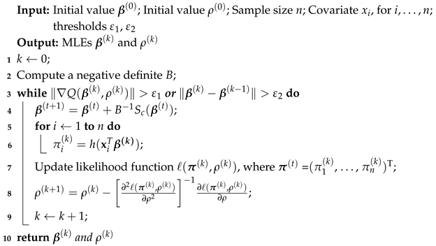
First, we analyze the estimators’ accuracy for given parameters under various link functions. Subsequently, we compare the algorithms. Then, we investigate the likelihood ratio test, Wald test, and score test under different link functions in terms of the type I error rates (TIEs) and powers.

3.1. Accuracy of the Estimators

In this subsection, we apply bias, average standard errors (ASE), and coverage probability (CP) to assess the point and interval estimates of the parameters $(\mathit{\beta },\rho )$. The bias measures the difference between the average MLEs of the parameters $(\mathit{\beta },\rho )$ and the corresponding actual values. The average standard errors mean the average of the standard errors of the MLEs. The coverage probability is a proportion of the asymptotic 95% confidence intervals for the parameters $(\mathit{\beta },\rho )$.

Take the sample size $n=200,400$ and correlation coefficient $\rho =0.3,0.5,0.7$. Other parameter settings are given according to the cases below:

Case (1). $q=2$, $\mathit{\beta }={(-1,2)}^{\mathrm{T}}$, ${\mathbf{x}}_i={(1,x_{i\left(1\right)})}^{\mathrm{T}}$, where ${\left\{x_{i\left(1\right)}\right\}}_{i=1}^n\stackrel{\mathit{i}.\mathit{i}.\mathit{d}.}{\sim }N(0.4,2.25\times {10}^{-2})$.

Case (2). $q=4$, $\mathit{\beta }={(-1,2,-1,2)}^{\mathrm{T}}$, ${\mathbf{x}}_i={(1,x_{i\left(1\right)},x_{i\left(2\right)},x_{i\left(3\right)})}^{\mathrm{T}}$, where ${\left\{x_{i\left(1\right)}\right\}}_{i=1}^n\stackrel{\mathit{i}.\mathit{i}.\mathit{d}.}{\sim }N(0.4,2.25\times {10}^{-2})$, ${\left\{x_{i\left(2\right)}\right\}}_{i=1}^n\stackrel{\mathit{i}.\mathit{i}.\mathit{d}.}{\sim }N(0.45,0.01)$, and ${\left\{x_{i\left(3\right)}\right\}}_{i=1}^n\stackrel{\mathit{i}.\mathit{i}.\mathit{d}.}{\sim }0.3+0.06\times t\left(5\right)$.

The samples $\left\{Y_i\right\}$ are generated randomly from the discrete distribution $Y_i\sim F_{Discrete}({(0,1,2)}^{\mathrm{T}},{\mathbf{p}}_i)$, where ${\mathbf{p}}_i={(p_{i0},p_{i1},p_{i2})}^{\mathrm{T}}$ depends on the specified link function. Once the samples are generated, the MLEs of the parameters $(\mathit{\beta },\rho )$ are computed following the estimation procedures detailed in Section 2 for each corresponding link function. In addition, the standard errors associated with the MLEs are also calculated to assess the variability of the parameter estimates. This simulation process is repeated 10,000 times for each link function, and the resulting values for bias, average standard error (ASE), and coverage probability (CP) are presented in

Table 3. Three metrics (%) of MLEs under the different link functions for Case (1).

$\mathit{\rho }$	MLEs	Index	n = 200					n = 400
			LL	CLL	L	DE	Pt	LL	CLL	L	DE	Pt
0.3	${\widehat{\beta }}_0$	Bias	−2.17	−1.15	−2.58	−2.13	−1.09	−2.13	0.05	−2.54	−1.23	−0.65
		ASE	31.8	23.7	111	24.0	20.8	24.8	17.3	85.2	18.2	15.9
		CP	95.5	95.4	95.5	95.6	95.3	95.1	94.7	95.3	94.9	95.2
	${\widehat{\beta }}_1$	Bias	5.27	2.65	6.94	4.43	2.33	4.97	0.25	6.30	3.16	1.91
		ASE	67.9	54.5	277	52.9	47.1	59.4	39.1	210	40.1	36.1
		CP	93.6	95.3	95.6	95.7	95.3	94.9	94.3	95.4	95.1	95.4
	$\widehat{\rho }$	Bias	−0.76	−0.71	−0.52	−0.53	−0.49	−0.44	−0.31	−0.29	−0.33	−0.32
		ASE	10.3	7.18	6.94	6.97	6.96	6.90	4.71	4.86	4.94	5.00
		CP	95.2	93.0	94.3	94.7	94.6	95.5	95.3	94.2	94.7	94.4
0.5	${\widehat{\beta }}_0$	Bias	−2.03	−0.84	0.56	−2.41	−1.10	−0.03	−0.07	−0.06	−0.65	−0.16
		ASE	26.9	26.7	145	30.1	26.6	17.6	18.5	90.5	18.7	16.3
		CP	95.2	94.8	95.1	94.6	94.8	95.3	95.2	95.1	94.4	94.8
	${\widehat{\beta }}_1$	Bias	4.28	1.76	−0.29	5.04	2.31	−0.34	0.35	−1.29	1.20	0.25
		ASE	60.1	59.5	356	65.0	59.2	38.5	40.9	224	41.0	37.2
		CP	94.9	94.8	94.5	94.6	95.0	95.2	95.2	94.7	95.2	94.4
	$\widehat{\rho }$	Bias	−3.30	−0.36	−0.35	−0.22	−0.22	−0.1	−0.23	−0.23	−0.17	−0.21
		ASE	6.35	6.36	6.22	6.24	6.19	4.45	4.46	4.32	4.47	4.47
		CP	93.3	94.7	94.3	95.6	95.6	95.2	94.8	94.5	94.7	94.9
0.7	${\widehat{\beta }}_0$	Bias	−1.19	−1.74	−1.40	−0.80	−1.36	−0.65	−1.44	−0.98	−1.81	−0.59
		ASE	26.5	29.3	39.3	27.7	25.4	19.6	19.3	29.3	20.1	17.3
		CP	94.5	93.9	95.2	94.0	94.9	94.3	95.2	94.9	95.0	95.1
	${\widehat{\beta }}_1$	Bias	2.88	3.78	2.67	4.07	2.61	1.80	2.91	2.22	2.24	0.95
		ASE	60.4	64.9	90.1	61.2	59.7	43.8	42.5	68.7	44.8	39.3
		CP	94.5	95.3	95.2	93.9	94.7	94.2	94.7	95.1	94.7	94.9
	$\widehat{\rho }$	Bias	−0.32	0.05	−0.23	−0.21	−0.16	−0.25	0.04	0.01	−0.02	−0.07
		ASE	5.19	5.13	6.00	6.63	5.21	3.61	3.68	3.59	4.59	3.79
		CP	94.8	94.3	94.4	93.9	94.6	95.0	95.1	94.5	94.9	94.5

Note. LL: Log–log, CLL: Complementary log–log, L: Logistic, DE: Double exponential, Pt: Probit.

and

Table 4. Three metrics (%) of MLEs under the different link functions for Case (2).

$\mathit{\rho }$	MLEs	Index	$\mathit{n}=200$					$\mathit{n}=400$
			LL	CLL	L	DE	Pt	LL	CLL	L	DE	Pt
0.3	${\widehat{\beta }}_0$	Bias	−2.62	−3.03	−8.37	−3.53	−1.17	−1.46	−1.54	−1.85	−3.3	−0.77
		ASE	59.1	45.2	74.3	53.5	53.4	37.3	36.9	55.5	34.2	33.9
		CP	93.7	95.2	94.6	94.9	94.5	95.6	95.1	95.3	94.9	94.8
	${\widehat{\beta }}_1$	Bias	2.15	3.59	4.42	6.59	3.23	1.43	1.33	3.35	2.04	2.68
		ASE	61.7	53.9	73.1	57.7	51.1	36.9	56.4	57.2	37.8	34.7
		CP	94.5	94.8	95.1	94.9	94.6	95.1	94.5	94.7	94.5	94.7
	${\widehat{\beta }}_2$	Bias	1.14	0.94	−2.08	−2.79	−3.01	−0.32	−0.87	−2.11	−0.63	−0.06
		ASE	79.5	74.9	124	72.6	76.9	56.4	52.1	83.3	49.9	54.6
		CP	94.8	94.8	94.3	95.3	94.6	95.3	94.7	95.4	95.7	94.5
	${\widehat{\beta }}_3$	Bias	6.98	7.65	23.9	6.92	2.48	0.75	2.09	5.64	3.83	1.99
		ASE	105	96.4	137	100	97.6	71.7	70.7	111	70.4	68.4
		CP	95.0	95.1	95.8	95.3	94.8	95.1	95.6	95.7	95.2	94.7
	$\widehat{\rho }$	Bias	−1.22	−1.19	−0.87	−0.97	−0.70	−0.45	−0.28	−0.45	−0.69	−0.34
		ASE	7.29	6.96	6.79	7.15	7.10	5.21	5.17	4.78	5.05	4.88
		CP	94.4	95.3	95.6	94.3	94.9	93.8	94.7	95.2	94.9	94.8
0.5	${\widehat{\beta }}_0$	Bias	−3.8	−2.83	−5.50	−5.95	−1.56	−2.16	−2.79	−1.14	−1.47	−0.11
		ASE	53.2	56.3	81.5	54.2	54.2	38.7	39.3	60.0	39.8	39.1
		CP	94.9	95.4	94.2	95.5	95.1	95.4	94.7	95.6	95.3	95.0
	${\widehat{\beta }}_1$	Bias	5.26	4.11	5.66	10.5	4.0	1.90	3.94	1.61	5.35	3.42
		ASE	60.0	56.6	79.7	58.3	55.8	37.0	44.0	61.1	43.8	38.9
		CP	94.2	94.8	95.4	94.3	94.5	95.8	94.4	95.1	94.3	94.6
	${\widehat{\beta }}_2$	Bias	−1.68	−1.64	1.02	−4.85	−4.24	0.50	−1.37	−0.83	−3.67	−1.03
		ASE	78.8	86.8	136	86.2	80.9	57.4	57.3	86.1	58.7	55.3
		CP	94.2	95.0	94.9	95.1	95.3	95.2	95.3	94.7	95.3	94.8
	${\widehat{\beta }}_3$	Bias	6.69	6.25	12.5	12.3	2.33	4.94	5.86	0.19	3.05	1.29
		ASE	106	99.2	152	107	103	75.9	73.5	123	77.1	74.4
		CP	94.4	95.2	95.4	96.0	94.5	94.6	94.7	94.2	95.5	94.8
	$\widehat{\rho }$	Bias	−0.56	−0.72	−0.66	−0.47	−0.43	−0.51	−0.32	−0.32	−0.40	−0.20
		ASE	6.64	6.42	6.45	6.44	6.43	4.76	4.55	4.42	4.54	4.48
		CP	95.1	95.6	93.6	94.4	94.7	95.0	95.1	95.3	94.8	95.3
0.7	${\widehat{\beta }}_0$	Bias	−4.37	−5.69	−9.83	−5.41	−4.15	−1.13	−1.57	−2.52	−1.83	−0.33
		ASE	60.3	59.5	84.0	57.6	56.9	42.9	38.6	63.8	42.6	38.1
		CP	94.6	94.8	94.5	95.0	94.9	94.5	95.2	95.9	95.2	94.5
	${\widehat{\beta }}_1$	Bias	6.30	5.67	6.33	9.61	4.16	2.21	2.35	5.06	2.91	2.43
		ASE	57.7	64.1	84.9	66.7	65.3	45.0	42.3	65.1	42.8	40.3
		CP	95.2	94.3	95.1	94.5	94.9	94.9	95.4	95.2	95.0	94.9
	${\widehat{\beta }}_2$	Bias	−2.79	−0.19	−4.13	−2.61	−2.38	0.12	−1.34	−3.43	0.60	0.27
		ASE	98.0	98.4	139	91.6	87.5	63.8	59.5	95.9	61.3	57.8
		CP	94.4	94.5	95.3	95.0	94.8	95.3	95.7	96.2	94.9	95.7
	${\widehat{\beta }}_3$	Bias	5.76	11.3	29.1	6.93	5.97	5.71	4.58	7.35	3.91	1.19
		ASE	117	121	157	119	112	78.9	79.1	127	88.4	78.9
		CP	94.5	95.4	96.4	95.2	94.8	95.8	94.7	95.6	95.0	95.0
	$\widehat{\rho }$	Bias	−0.38	−0.51	−0.54	−0.71	−0.57	−0.19	−0.21	−0.27	−0.37	−0.21
		ASE	5.56	5.36	5.24	5.91	5.27	3.77	3.75	3.36	4.29	3.78
		CP	94.1	94.6	94.7	95.0	95.1	95.4	95.2	95.1	94.5	94.7

Note. LL: Log–log, CLL: Complementary log–log, L: Logistic, DE: Double exponential, Pt: Probit.

.

Table 3 shows that the values of the three evaluation metrics, bias, ASE, and CP, fall within acceptable and reasonable ranges. As the sample size increases, while keeping other parameters constant, both the bias and ASE of the parameters $(\mathit{\beta },\rho )$ decrease under all five link functions. A closer analysis of the three metrics across different link functions reveals that, for a fixed sample size and correlation coefficient, the logistic link function tends to exhibit the highest ASE for the parameter $\mathit{\beta }$. However, when using the Fisher bounded algorithm to estimate $\mathit{\beta }$, the ASE is lower than the other link functions, suggesting that the Fisher bounded algorithm performs better than the QLB algorithm in estimation accuracy.

Further examination of the probit link function shows that the estimated parameters $(\mathit{\beta },\rho )$ demonstrate smaller bias and lower ASE, with the CP ranging from 94% to 96%, which is within an acceptable range. In contrast, under the DE link function, when $\rho$ = 0.7 and n = 400, the bias and ASE for the parameters $(\mathit{\beta },\rho )$ are higher. Additionally, for smaller sample sizes, under the log–log and complementary log–log link functions, the CP for the parameters $(\mathit{\beta },\rho )$ ranges from 93% to 97%, which is slightly wider than the CP observed for the probit link function.

As shown in Table 4, the overall performance for Case (2) is quite similar to that observed in Case (1). The logistic link function shows the largest ASE for $\mathit{\beta }$. The three metrics demonstrate a more pronounced advantage for the probit link function than other link functions. While the CP for $(\mathit{\beta },\rho )$ improves under the complementary log–log link function, the bias and ASE are still higher than those for the probit link function. The performance of the double exponential and log–log link functions remains similar to that observed in Case (1), with comparable results for the three metrics.

In summary, all five link functions perform within an acceptable range, validating the algorithm’s convergence. The probit link function demonstrates the most robust performance and can be considered the preferred choice. The logistic link function exhibits a higher ASE related to the algorithm. The performance of the CLL and LL link functions fluctuates significantly, reflecting each link function’s characteristic suitability for extreme event probabilities. The DE link function shows poor stability under high correlation and large sample sizes.

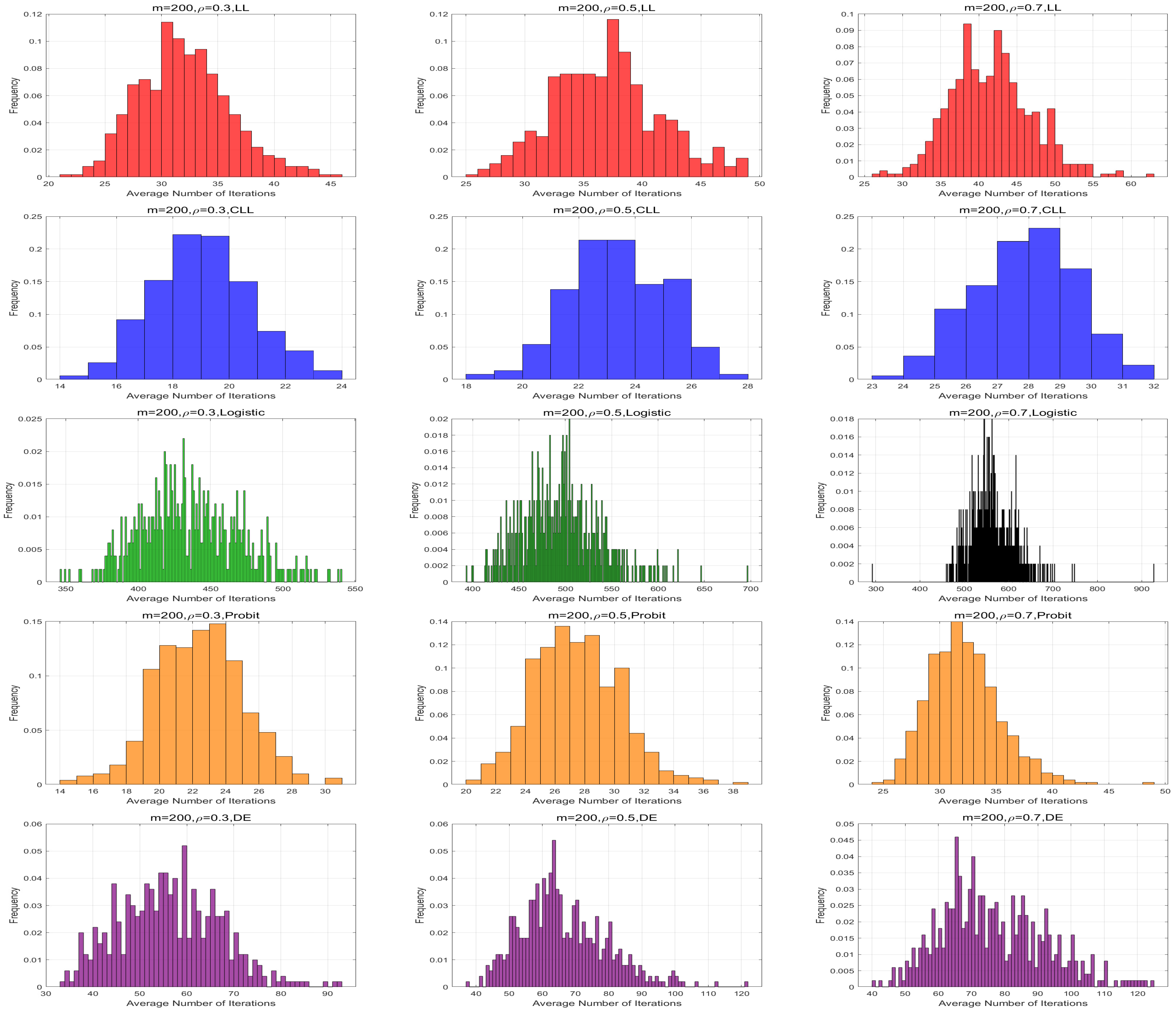
3.2. Comparison of Algorithms

Under various link functions, we compare the effectiveness of algorithms by the average iteration count and the computing time. An algorithm is considered more efficient if it achieves a desired level of accuracy with fewer iterations or in less computation time.

Let $m=200,400$, and $\rho =0.3,0.5,0.7$, and the other parameter settings refer to Case (1). The samples $\left\{Y_i\right\}$ are randomly generated from the discrete distribution $Y_i\sim F_{Discrete}({(0,1,2)}^{\mathrm{T}},{\mathbf{p}}_i)$, where ${\mathbf{p}}_i={(p_{i0},p_{i1},p_{i2})}^{\mathrm{T}}$ depends on the specified link function. Regarding parameter estimations, we use the QLB-based NR algorithm with the logistic link function, while for the other four link functions, we employ the Fisher-bound-based NR algorithm. All experiments were repeated 500 times.

Figure 1 and Figure 2 provide the frequency distributions of the average iteration numbers under the different link functions. The average number of iterations under the logistic link function is significantly higher than that of the other four link functions across all parameter settings. On the other hand, we fixed the iteration number to 100 and recorded their time cost. The average iteration time for five link functions is shown in

Table 5. Comparison of the average iteration time (ms) under five link functions.

n	$\mathit{\rho }$	LL	CLL	L	DE	Pt
200	0.3	6.19	5.30	11.9	7.75	5.56
	0.5	7.26	6.24	12.3	9.25	6.34
	0.7	8.15	7.06	13.1	10.1	7.28
400	0.3	54.2	46.7	104	70.8	47.2
	0.5	63.1	49.3	115	80.2	57.1
	0.7	74.1	50.7	146	87.4	68.3

Note. LL: Log–log, CLL: Complementary log–log, L: Logistic, DE: Double exponential, Pt: Probit.

. Under all parameter settings, the average iteration time for the logistic link function is also notably longer than for the other link functions.

These findings suggest that the computational performance of the Fisher-bound-based NR algorithm is substantially more efficient than the QLB-based NR algorithm. Through comparisons across different link functions, we observe that both the average number of iterations and the average computation time increase with the sample size and the correlation coefficient. This demonstrates that both factors have a significant impact on the computational burden of the algorithms. Moreover, it is worth noting that the Fisher-bound-based NR algorithm with the CLL link function consistently exhibits the best performance across all parameter settings.

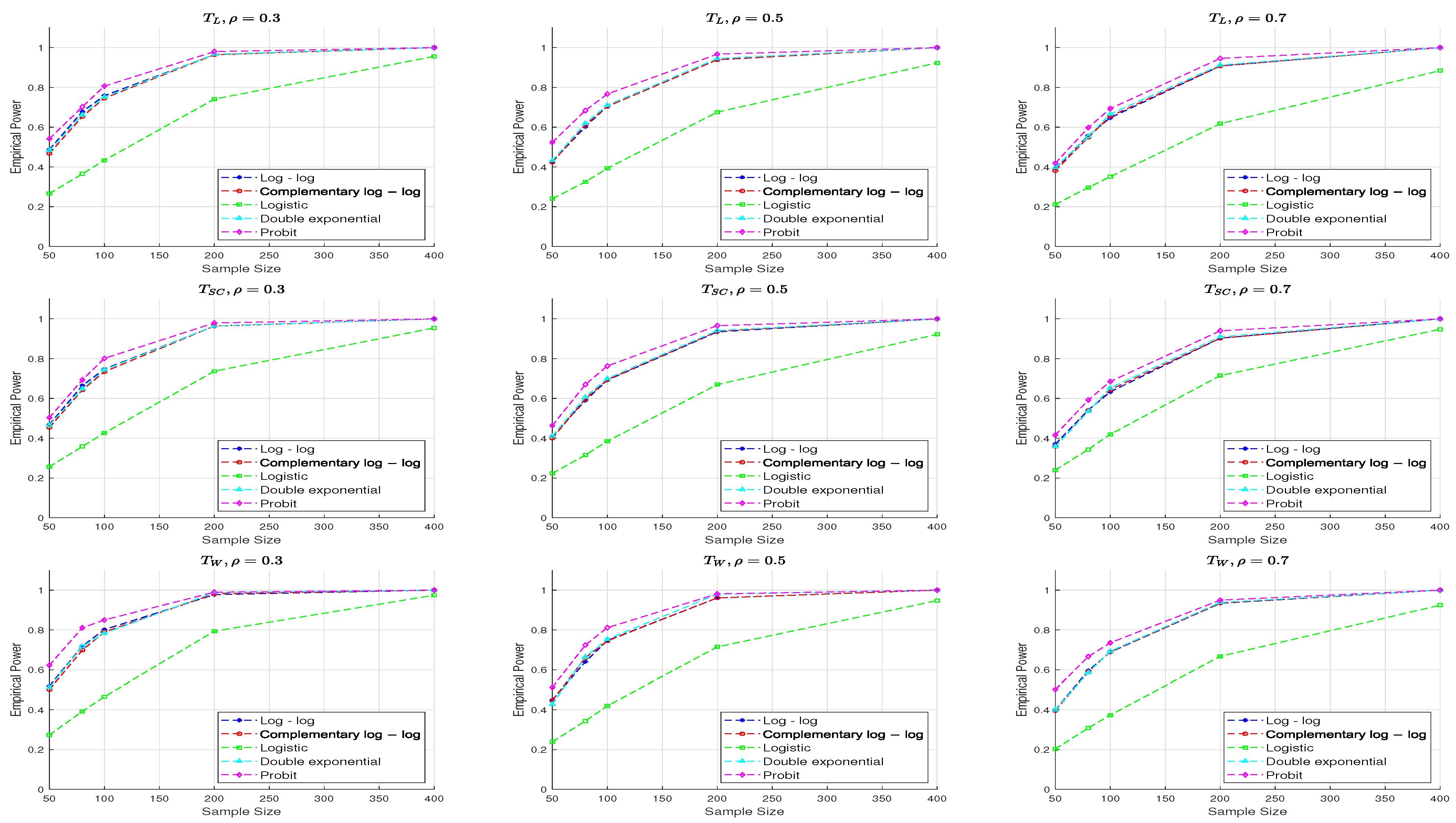
3.3. Comparison of Test Statistics

Under the hypothesis test (5), we evaluate the performance of the three statistics for given link functions with parameter settings. Take the sample size $n=200,400$ and the correlation coefficient $\rho =0.3,0.5,0.7$. The covariate vector ${\mathbf{x}}_i$ is defined in Cases (1) and (2). Other parameter settings are based on the two cases: (I) $q=2$, $\mathit{\beta }={({\beta }_0,{\beta }_1)}^{\mathrm{T}}$, ${\beta }_0={\beta }_1=0$, $C=\left(1,-1\right)$. (II) $q=4$, $\mathit{\beta }={({\beta }_0,{\beta }_1,{\beta }_2,{\beta }_3)}^{\mathrm{T}}$, ${\beta }_0={\beta }_1={\beta }_2={\beta }_3=0$, and

$$C=\left(\begin{array}{cccc}1& -1& 0& 0\\ 0& 1& -1& 0\\ 0& 0& 1& -1\end{array}\right).$$

Similarly, the samples $\left\{Y_i\right\}$ are generated from the discrete distribution $F_{Discrete}({(0,1,2)}^{\mathrm{T}},{\mathbf{p}}_i)$ for 10,000 times, where ${\mathbf{p}}_i=$${(p_{i0},p_{i1},p_{i2})}^{\mathrm{T}}$. The empirical type I error rate is calculated by dividing the number of rejections of the null hypothesis $H_0$ by the total number of simulations, which is 10,000. The empirical TIEs are summarized in

Table 6. Empirical type I error rates (%) for Case (I) and Case (II) under the different link functions.

n	$\mathit{\rho }$	Statistics	Case (I)					Case (II)
			LL	CLL	L	DE	Pt	LL	CLL	L	DE	Pt
200	0.3	TL	5.0	5.3	4.8	4.7	5.6	5.4	4.7	4.8	5.2	5.0
		TW	5.3	5.4	4.8	3.3	5.0	4.8	4.8	4.7	3.7	4.7
		TSC	5.3	5.4	4.7	4.8	4.8	4.7	5.0	4.9	4.9	4.6
	0.5	TL	5.4	4.5	5.2	5.0	5.1	5.3	4.8	5.0	5.2	4.8
		TW	5.4	5.1	4.9	3.7	5.3	5.3	4.8	4.9	4.0	4.9
		TSC	5.1	5.2	4.7	4.9	4.6	5.1	4.6	4.8	5.1	5.1
	0.7	TL	4.8	5.4	4.7	4.7	5.2	5.2	5.1	4.8	5.5	4.8
		TW	5.2	4.6	5.5	2.9	5.2	5.2	5.0	4.8	4.1	4.8
		TSC	5.0	5.0	5.4	4.8	5.2	4.7	5.5	4.7	5.4	4.7
400	0.3	TL	4.7	4.8	5.2	5.0	5.2	4.7	4.8	5.2	5.0	5.2
		TW	4.8	4.8	4.7	3.7	4.7	4.8	4.8	4.7	3.7	4.7
		TSC	4.7	5.0	4.9	4.9	4.6	4.7	5.0	4.9	4.9	4.6
	0.5	TL	5.3	4.8	5.0	5.2	4.8	5.3	4.8	5.0	5.2	4.8
		TW	5.4	5.1	4.9	3.7	5.3	5.3	4.8	4.9	4.0	4.9
		TSC	5.1	4.6	4.8	5.1	5.1	5.1	4.6	4.8	5.1	5.1
	0.7	TL	5.2	5.1	4.8	5.5	4.8	5.2	5.1	4.8	5.5	4.8
		$T_W$	5.2	5.0	4.8	4.1	4.8	5.2	5.0	4.8	4.1	4.8
		$T_{SC}$	4.7	5.5	4.7	5.4	4.7	4.7	5.5	4.7	5.4	4.7

Note. LL: Log–log, CLL: Complementary log–log, L: Logistic, DE: Double exponential, Pt: Probit.

. Power refers to the probability of correctly rejecting the null hypothesis $H_0$ when it is false. We consider sample sizes n = 50, 80, 100, 200, 400, and $\rho$ = 0.3, 0.5, 0.7. The following two cases of regression coefficient vectors are considered: (A) $\mathit{\beta }={(-1,2)}^{\mathrm{T}}$ and (B) $\mathit{\beta }={(-1,2,-1,2)}^{\mathrm{T}}$. The other parameter configurations remain consistent with Cases (I) and (II). For each $i=1,\dots ,n$, we generate $Y_i\sim F_{Discrete}({(0,1,2)}^{\mathrm{T}},{\mathbf{p}}_i)$ 10,000 times, where ${\mathbf{p}}_i={(p_{i0},p_{i1},p_{i2})}^{\mathrm{T}}$. The empirical power of each test is computed as the proportion of rejections at the 0.05 significance level over 10,000 simulations. 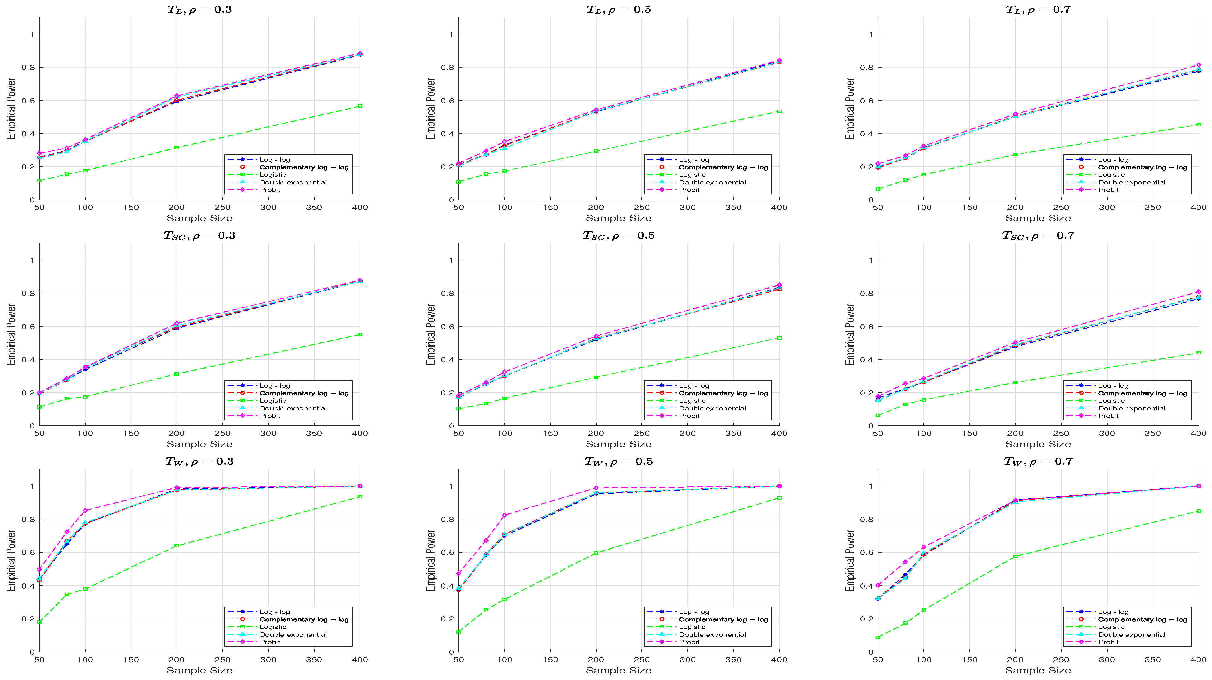Figure 3 and Figure 4 display the empirical powers of the three test statistics across five different link functions. A comparison of the results shows that both the $T_L$ and $T_{SC}$ tests consistently maintain empirical type I error rates (TIEs) close to the nominal level of 0.05 across all link functions considered (LL, CLL, L, DE, and Pt), indicating robust performance. In contrast, the $T_W$ test tends to yield lower empirical TIEs under the double exponential link, though its TIEs for other link functions fluctuate around the nominal level. Furthermore, empirical TIEs are generally higher when $q=4$ compared to $q=2$, with this effect being more noticeable for smaller sample sizes.

Figure 3 illustrates that increasing the sample size enhances the power of all three test statistics. Power decreases slightly for a fixed sample size as $\rho$ increases. The $T_W$ statistic demonstrates the best performance, while $T_L$ and $T_{SC}$ produce comparable results across all parameter settings. Among the link functions, the probit link generally yields the highest power, especially for small sample sizes, whereas the logistic link results in the lowest. The log–log, complementary log–log, and double exponential links exhibit similar power levels.

From Figure 4, we observe that the performance of the three test statistics for $q=4$ is generally similar to that for $q=2$, though there are some differences. Specifically, compared to $q=2$, the power of all test statistics decreases when $q=4$, with the $T_L$ and $T_{SC}$ test statistics showing a more pronounced decline across all parameter settings and link functions.

In addition to the empirical findings, theoretical analysis suggests that the Wald test achieves higher power under the probit link due to its derivative structure, which yields greater Fisher information and a larger non-centrality parameter $\lambda$ [30].

Moreover, considering that the $T_W$ test statistic under the probit link function shows robust empirical TIEs, it is recommended as the most effective test for assessing the significance of confounding effects on the response rate.

4. An Application

In this section, we analyze a dataset from a survey conducted in the Varamin region of Iran, focusing on individuals aged 50 and above with visual impairment [31]. The dataset includes nearly 3000 participants, categorized into seven groups ($g=1,2,\dots ,7$). Responses are recorded as no blindness, unilateral blindness, or bilateral blindness ($l=0,1,2$). The dataset’s structure is presented in

Table 7. Prevalence of blindness by age groups ($g=7$).

Age (g)	Blindness (l)
	None (0)	Unilateral (1)	Bilateral (2)
50–54 yrs	964	23	2
55–59 yrs	541	17	8
60–64 yrs	469	18	4
65–69 yrs	257	16	5
70–74 yrs	242	32	3
75–79 yrs	127	30	9
80+ yrs	104	29	10

. Since the response probabilities in our model are defined at the individual level, we preprocess the data as follows to ensure analytical accuracy and consistency:

(1)

Use the midpoints of the age groups as a proxy for age to account for potential confounding.

(2)

Assume that individuals within the same group share identical covariates, resulting in uniform response rates within each group;

(3)

Scale all data values by a factor of 1/100 to reduce the impact of magnitude differences on computation.

We construct a generalized linear model to explore the relationship between age and disease rates. The model incorporates five link functions specified in Section 2. The MLEs of $(\beta ,\rho )$, their standard errors (SE), and the asymptotic 95% confidence interval widths (CIW) can be computed using the method described in Section 3 under the corresponding link function.

As shown in

Table 8. Parameter estimates under different link functions.

Index	Parameters	LL	CLL	L	DE	Pt
MLE	${\beta }_0$	−7.984	2.960	−9.003	−8.842	−4.401
	${\beta }_1$	0.084	−0.029	0.091	0.088	0.042
	$\rho$	0.272	0.274	0.273	0.272	0.272
SE	${\beta }_0$	0.156	0.487	0.506	0.467	0.229
	${\beta }_1$	0.242	0.453	0.073	0.066	0.034
	$\rho$	0.041	0.041	0.041	0.077	0.041
CIW	${\beta }_0$	0.612	1.910	1.980	1.830	0.898
	${\beta }_1$	0.948	0.178	0.286	0.259	0.133
	$\rho$	0.159	0.159	0.159	0.159	0.159

Note. LL: Log–log, CLL: Complementary log–log, L: Logistic, DE: Double exponential, Pt: Probit.

, $\widehat{\rho }$ is approximately 0.273 under all link functions, indicating a positive correlation between the responses of both eyes of a patient. Among them, the Pt model exhibits the lowest standard errors and the narrowest confidence intervals, demonstrating the most robust performance. The LL link function and the DE link function yield similar results. Still, the LL link function is slightly better because it is more suitable for modeling low probability events, which aligns with the dataset’s characteristics [32]. In contrast, the CLL link function is designed for modeling high-probability events, leading to inconsistencies between the model assumptions and the data characteristics, resulting in a negative regression coefficient. The L link function has the largest standard error for the intercept coefficient. As shown in

Table 9. Values of AIC and BIC under different link functions.

Tests	LL	CLL	L	DE	Pt
AIC	1540.8	1544.8	1540.9	1542.6	1540.7
BIC	1558.7	1560.6	1562.8	1558.9	1558.6

Note. LL: Log–log, CLL: Complementary log–log, L: Logistic, DE: Double exponential, Pt: Probit.

, the Q-Q plots and residual plots under all link functions show little difference. Overall, the models appear to provide similar fits. Furthermore, according to the AIC and BIC results (Figure 5), the Pt model demonstrates the best fitting efficiency among all the models. Given the low disease probability in this dataset [32], which does not match the overall assumptions of the simulated data, different link functions significantly impact the parameter estimation results, particularly for ${\beta }_0$ and ${\beta }_1$. However, the conclusions drawn from the model comparisons are consistent with those from the simulation study.

Lastly, we need to test the hypothesis (5), where $C=(0,1)$ and $\mathit{\beta }={({\beta }_0,{\beta }_1)}^{\mathrm{T}}$. The values of the three statistics $T_L,T_W,$ and $T_{SC}$ are shown in

Table 10. Values of three statistics under different link functions.

Tests	Results	LL	CLL	L	DE	Pt
$T_L$	Statistic	152.404	158.871	158.713	158.967	156.832
	p-value	5.17 × ${10}^{-35}$	2.00 × ${10}^{-36}$	2.16 × ${10}^{-36}$	1.90 × ${10}^{-36}$	5.57 × ${10}^{-36}$
$T_W$	Statistic	226.148	223.229	215.056	213.505	232.597
	p-value	4.13 × ${10}^{-51}$	1.79 × ${10}^{-50}$	1.08 × ${10}^{-48}$	1.90 × ${10}^{-36}$	5.57 × ${10}^{-36}$
$T_S$	Statistic	178.743	178.743	178.743	178.742	178.743
	p-value	9.12 × ${10}^{-41}$	9.12 × ${10}^{-41}$	9.12 × ${10}^{-41}$	9.12 × ${10}^{-41}$	9.12 × ${10}^{-41}$

Note. LL: Log–log, CLL: Complementary log–log, L: Logistic, DE: Double exponential, Pt: Probit.

. The test statistic $T_W$ values vary slightly with different link functions, and the test statistic $T_L$ exhibits a similar pattern. In contrast, the $T_{SC}$ test statistic remains consistent under all link functions. This indicates that the choice of link function significantly impacts some statistics but has little impact on others. Under all link functions, the values of the $T_W$ test statistic are greater than the other two, indicating that the $T_W$ test statistic performs better. Since all p-values are less than 0.05, we reject the null hypothesis and conclude that age significantly affects disease rates. Similarly, this result is consistent with the observations in the simulation.

5. Discussion and Conclusions

This paper develops a generalized linear model to investigate the relationship between confounding effects and response rates. Since the log-likelihood function involving various link functions is generally non-concave, we adopt a novel MM algorithm to construct a surrogate function that approximates the logistic log- ikelihood, ensuring computational feasibility and stability. Five specific link functions are considered: log–log, complementary log–log, logistic, double exponential, and probit. We also describe three parameter estimation methods: the NR, QLB, and Fisher-bounded algorithms. Additionally, three hypothesis testing procedures, the likelihood ratio test, the Wald test, and the score test, are introduced to assess the significance of regression coefficients under different link functions. Simulation results indicate that, regardless of the link function or estimation method, the MLEs closely approximate the actual values, and the corresponding confidence intervals fall within reasonable bounds. In terms of convergence, the Fisher bounded algorithm outperforms the others. Comparison of the test statistics reveals that the point and interval estimates of $(\mathit{\beta },\rho )$ are the most accurate under the probit link function. Under the double exponential link, the empirical type I error rate of $T_W$ is notably lower than the nominal level, while $T_L$ and $T_{SC}$ remain close to 0.05. All three tests control type I error for the other link functions. Furthermore, $T_W$ consistently demonstrates the highest statistical power across all scenarios, increasing power as the sample size grows. We therefore recommend the use of $T_W$. The logistic link yields the lowest power among the five link functions, while the probit link yields the highest. Finally, the proposed method is applied to real data from a study of visually impaired individuals in Iran, demonstrating its practical applicability and effectiveness.

Lin et al. [23] used a logistic regression to study the relationship between ophthalmic disease prevalence and patient covariates. It combines the fast QLB algorithm with coordinate ascent to compute the unconstrained MLE of the parameters of interest. Compared with the existing results, our proposed model offers greater generalization ability and achieves better performance in terms of computational efficiency and applicability. Simulation studies and real-data analyses further validate this assumption, demonstrating the practical advantages of our method. In addition, Li et al. [5] proposed a flexible beta-kernel correlation model capable of fitting binary data with a wide range of correlation structures. Compared to our method, their model only shows superior performance in certain scenarios.

The method proposed in this paper can be extended to other intra-class models such as Rosner’s or Dallal’s model and supports both unilateral and bilateral data structures. However, some unsolved problems exist, such as complex correlations, binary-only outcomes, and small sample behavior. Moreover, the model dependence between random vectors is conducive to more comprehensively capturing the information between covariates. However, our current method has not yet constructed the joint distribution of random variables, and thus it is difficult to delve into the specific relationships between variables. Moreover, we have only focused on the individual distributions of random variables. Future research can further construct the joint distribution of random variables to explore the specific relationships between them thoroughly. Based on [33], we can model the dependence between random vectors, thereby comprehensively capturing all the information between covariates. These are important directions for future research, and we will further investigate these interesting issues in the general case.