Abstract
This article presents maximum likelihood and Bayesian estimates for the parameters, reliability function, and hazard function of the Gumbel Type-II distribution using a unified hybrid censored sample. Bayesian estimates are derived under three loss functions: squared error, LINEX, and generalized entropy. The parameters are assumed to follow independent gamma prior distributions. Since closed-form solutions are not available, the MCMC approximation method is used to obtain the Bayesian estimates. The highest posterior density credible intervals for the model parameters are computed using importance sampling. Additionally, approximate confidence intervals are constructed based on the normal approximation to the maximum likelihood estimates. To derive asymptotic confidence intervals for the reliability and hazard functions, their variances are estimated using the delta method. A numerical study compares the proposed estimators in terms of their average values and mean squared error using Monte Carlo simulations. Finally, a real dataset is analyzed to illustrate the proposed estimation methods.
Keywords:
unified hybrid censoring schemes; Gumbel Type-II distribution; frequentist estimation; Bayesian inference; COVID-19 MSC:
62N01; 62N02; 62F10
1. Introduction
In lifetime experiments, censoring is commonly used to address time and cost constraints, especially when testing modern, highly reliable items that require long testing periods in conventional studies. Various censoring techniques are applied in real-world scenarios with different objectives to improve efficiency and reduce unnecessary expenses. Censoring is widely used in fields such as clinical trials, biological studies, and industrial engineering. Two of the most commonly used methods are type-I and type-II censoring schemes, where testing ends at a predetermined time T or upon the occurrence of the r-th failure, respectively.
Epstein [1] introduced a hybrid Type-I censoring method in which the experiment ends at , where represents the failure time of the r-th unit. In contrast, Childs et al. [2] proposed a Type-II hybrid censoring scheme that terminates at . However, both Type-I and Type-II censoring methods share the same limitations as the Type-II hybrid censoring technique. To address these constraints, Chandrasekar et al. [3] introduced two generalized hybrid censoring methods. Although these approaches were designed to overcome the issues associated with Type-I and Type-II hybrid censoring schemes, they still have certain drawbacks. For instance, in the generalized Type-I hybrid censoring approach, the experimenter may fail to observe the r-th failure within the specified time frame.
To tackle these issues, Balakrishnan et al. [4] developed unified hybrid censoring methods (UHCS). The parameters of a life testing experiment with n objects are predetermined by the experimenter in the UHCS. k and , where , and , are the preset values. However, if the k-th failure happens before , the experiment stops at . Should the k-th failure take place between and , the experiment is ended at . If the k-th failure happens after , the experiment is terminated at . Due to the significance of this type of information, a number of authors have studied this topic, namely [5,6,7,8,9,10,11,12].
Consequently, we determine the six scenarios in Table 1 in respect to the UHCS.

Table 1.
Situations where UHCS analyzing will be finished.
The likelihood function in accordance with the UHCS is
where
In this case, Q and A stand for the total number of test failures up until the end of time, respectively.
When analyzing real-world data on COVID-19 patient mortality rates, we often encounter information related to the time until a specific event occurs. Such data, commonly referred to as survival time data, typically exhibit a right-skewed distribution. The Gumbel Type-II distribution (G-IID), known for its positive skewness, is well-suited for modeling this type of data. Introduced by the German mathematician Gumbel [13], the G-IID has proven valuable for modeling extreme events, including floods, earthquakes, and other natural disasters. Its applications extend to life expectancy tables, hydrology, and rainfall studies. Gumbel himself demonstrated the effectiveness of this distribution in simulating expected lifespans during product lifetime comparisons. Additionally, the G-IID plays a crucial role in predicting the probabilities of natural hazards and meteorological phenomena.
Substantial progress has been made in statistical inference methods for the G-IID. For instance, Mousa et al. [14] investigated Bayesian estimation through simulations based on specific parameter values. Nadarajah and Kotz [15] enhanced the beta Gumbel distribution and proposed maximum likelihood algorithms, and Miladinovic and Tsokos [16] examined Bayesian reliability estimation for a modified Gumbel failure model using the square error loss function.
Focusing specifically on the G-IID, Feroze and Aslam [17] investigated Bayesian estimation methods for doubly censored samples under various loss functions. Abbas et al. [18] expanded the scope of inference by incorporating Bayesian estimation approaches for the G-IID. The Bayesian estimation of two competing units within this distribution was derived by Feroze and Aslam [19]. Reyad and Ahmed [20] estimated unknown shape parameters for joint Type-II censored data using Bayesian and E-Bayesian approaches. Sindhu et al. [21] examined Bayesian estimators and their associated risks under diverse informative and non-informative priors for left Type-II censored samples. Additionally, Abbas et al. [22] applied Lindley’s approximation to develop Bayesian estimators for Type-II censored data under a non-informative prior and multiple loss functions. More recently, Qiu and Gui [23] derived Bayesian estimates for two G-IID under joint Type-II censoring. For and , the G-IID’s cumulative distribution function (CDF) is as described below:
additionally, the probability density function (PDF) that corresponds to it is given as follows:
The reliability function is defined as
and the failure rate function is expressed as follows:
In this context, the parameters and denote shape and scale, respectively.
Figure 1 shows the PDF, while Figure 2 illustrates the CDF of the G-IID for different values of the parameter , with held constant. The G-IID was selected for this analysis due to both its theoretical properties and empirical performance in modeling positively skewed, heavy-tailed lifetime data. This type of distribution is well-suited for capturing the nature of COVID-19 mortality data, which often exhibits a long right tail reflecting delayed fatalities or rare high-mortality days during outbreak peaks.
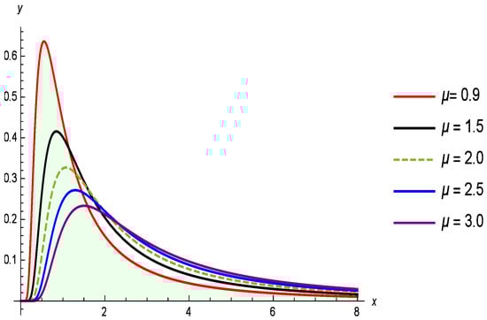
Figure 1.
Illustrates how the PDF of the G-IID varies with the parameter and .
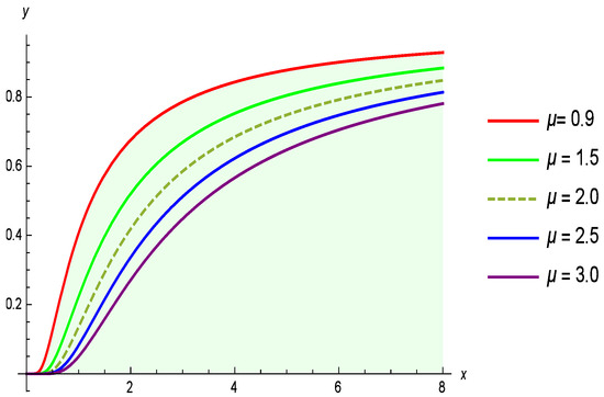
Figure 2.
Illustrates how the CDF of the G-IID varies with the parameter and .
1.1. Why G-IID over Weibull, Gompertz, or GEV?
- The Weibull distribution is widely used but often underestimates the probability of extreme outcomes due to its limited tail flexibility.
- The Gompertz distribution, while biologically interpretable, is more appropriate for modeling aging-related hazards rather than acute, outbreak-driven data.
- The Generalized extreme value (GEV) family is flexible but contains three parameters and may overfit small or moderately censored samples; in contrast, G-IID offers a parsimonious two-parameter alternative with similar right-tail behavior.
The Gumbel Type-II’s cumulative distribution function reflects a heavy right tail and positive skewness. The shape parameter controls the degree of skewness, while the scale parameter affects the spread. This flexibility allows the model to capture rare but significant increases in mortality; such as spikes due to emerging variants or delayed healthcare responses.
1.2. Interpretation of Parameters
- Higher values of correspond to sharper declines in the hazard rate, suggesting more concentrated mortality during epidemic peaks.
- Lower values of reflect long-tail behavior, i.e., mortality tapering off slowly rather than abruptly.
These properties make the G-IID suitable not only from a statistical fitting perspective but also for capturing the practical dynamics of COVID-19 mortality trends.
This research aims to develop and evaluate estimation methods for the parameters, reliability function, and hazard function of the G-IID under UHCS. It contributes by applying both classical and Bayesian approaches to estimate unknown parameters using real and simulated data. The study derives maximum likelihood estimators (MLEs), constructs asymptotic confidence intervals (ACIs) using the Fisher information matrix, and obtains Bayesian estimates under three distinct loss functions: squared error (SE), LINEX, and generalized entropy (GE). Since analytical Bayesian estimates are not available, the research utilizes Markov Chain Monte Carlo (MCMC) methods, including Metropolis–Hastings within Gibbs sampling, to generate posterior estimates and credible intervals. Through extensive simulation studies and real data application, the study highlights the efficiency and reliability of Bayesian methods, particularly under the GE loss function, in handling censored lifetime data. The work offers a practical and flexible framework for improving reliability analysis and life-testing experiments, providing new insights into the modeling of incomplete or censored data using the G-IID.
This study contributes to the Special Issue’s focus by addressing the challenge of making reliable inferences from censored and incomplete data. Using unified hybrid censoring schemes and real pandemic data, we demonstrate robust statistical estimation techniques that support uncertainty modeling and decision making in applied sciences.
The manuscript makes a substantial contribution to the field of reliability analysis and life-testing experiments by applying a UHCS alongside Bayesian estimation methods. To clarify its novelty, the work integrates both Type-I and Type-II censoring into a single unified framework, offering greater flexibility than previous studies that typically treated these schemes separately. While hybrid censoring has been applied to Gumbel-related distributions before, the unified approach presented here accommodates a wider range of experimental conditions. Additionally, the manuscript distinguishes itself through its application of Bayesian estimation under multiple loss functions—squared error, LINEX, and generalized entropy—unlike prior studies that often relied solely on maximum likelihood estimation (MLE) with a single loss criterion. The rationale for adopting Bayesian methods is well-founded; Bayesian inference allows for the incorporation of prior information and yields credible intervals, enhancing the reliability of estimates, especially under censored data scenarios, such as COVID-19 mortality datasets. These advantages are further highlighted by the limitations of MLE, including its potential bias in small samples and instability under heavy censoring, which can lead to large variances and unreliable estimates. In contrast, Bayesian methods maintain consistent performance under extreme censoring and offer robustness critical for practical applications. To reinforce this point, the manuscript would benefit from addressing the weaknesses of MLE explicitly in the Introduction. Doing so would provide a clearer rationale for the methodological choices made and prepare readers for the simulation-based comparisons discussed later. This framing would enhance the coherence of the argument and highlight the practical and theoretical strengths of the Bayesian approach within the context of the G-IID and UHCS.
This paper proceeds as follows. Section 2 provides the survival and hazard rate functions, as well as the MLEs for the unknown parameters. The Fisher information matrix (FIM) is used to create ACIs for interval estimation in Section 3. Bayesian parameter estimation using Gibbs sampling and importance sampling strategies under three distinct loss functions is shown in Section 4. A real dataset is analyzed in Section 5 to investigate parameter estimation. Section 6 presents a Monte Carlo simulation analysis to evaluate the proposed estimates based on average width, mean squared error (MSE), and average value. Finally, Section 7 provides the conclusions.
2. Maximum Likelihood Estimation
Assume that the random sample is drawn from the G-IID. By incorporating Equations (2) and (3) into Equation (1) and omitting the constant term, the likelihood function is given by
where is constant.
Using Equation (7), the log-likelihood function for and is expressed as
Differentiating Equation (8) with respect to and gives the following partial derivatives of the likelihood function:
Simultaneously solving the complex nonlinear Equations (9) and (10) enables the estimation of the MLEs for and . However, deriving explicit closed-form solutions for these equations is difficult. Therefore, numerical methods, such as the Newton–Raphson algorithm, are used to compute the MLEs of the unknown parameters. Additionally, the consistency property of MLEs allows for the estimation of and at a given time t. To determine these MLEs, substitute the estimated values and into Equations (2) and (3), respectively.
and
3. Fisher Information Matrix
To construct the ACIs in this subsection, the asymptotic variance–covariance matrix is required. This matrix is obtained by inverting the FIM. The inverse of the FIM is given as follows:
However, deriving exact mathematical expressions for these assumptions is challenging. For further details, refer to Cohen [24]. As a result, the asymptotic variance–covariance matrix is given as follows:
Since the MLEs are asymptotically normal, ACIs can be constructed for the parameters and . The ACIs for these parameters are given by:
Greene [25] provides a detailed explanation of the delta method, a general approach for computing ACIs for functions of MLEs. This method is used to estimate the variances of and , which depend on the parameters and , to construct the corresponding ACIs. Consequently, the variances of and are provided as follows:
The gradients of and with regard to and , respectively, are represented by in these formulas with regard to and , respectively. Consequently, the ACIs for and are calculated as follows:
4. Bayes Estimation
The fact that the Bayes estimate simultaneously considers the information from observed sample data and the prior information sets it apart from MLE. In a more reasonable and logical manner, it can describe the issues, considering the independent Gamma distributions of the parameters and
where and serve as hyperparameters. Consequently, the following is an expression for the joint prior distribution for and :
Using Equations (7) and (13), the joint posterior density function for and is as follows:
It is not possible to simply calculate the Bayes estimator from Equation (14) using mathematical techniques. In order to generate crucial estimators for and , as well as and , and their respective credible intervals (CRIs), the MCMC technique should be utilized. Two practical MCMC techniques that have been applied extensively in statistics are Metropolis–Hastings (M-H) and Gibbs sampling.
Metropolis–Hastings with Gibbs Sampler Algorithm
The M-H with Gibbs sampler algorithm is used to generate samples from complex probability distributions when the conditional distribution of each variable is available, but the joint distribution is unknown or difficult to handle. This technique applies the Gibbs sampler when conditional distributions are easy to sample from, while incorporating M-H in steps where direct sampling is not feasible. Its importance lies in handling high-dimensional models or cases where conditional distributions are non-standard, making direct sampling impractical. This approach is widely used in Bayesian inference, providing approximate estimates of posterior distributions for unknown parameters, thereby facilitating the analysis of complex data and statistical estimation efficiently. For the parameters and , the conditional posterior distributions are as follows:
In this instance, the distribution of is . To do this, the Gibbs sampler must be used to create random samples for . Direct sampling using conventional methods is also not feasible since the conditional posterior distribution of cannot be analytically simplified into standard distributions. The M-H technique, which uses a normal proposal distribution, is utilized to generate samples. To evaluate the samples for and , the following algorithm can be used.
- 1: Let be the starting values, and let B represent the burn-in time.
- 2: Put .
- 3: Use to generate .
- 4: By using Equations (16), can be generated using the M-H approach. A normal distribution such as is advised. The inverse FIM’s major diagonal can be used to compute in this case.(I) Calculate the rate of acceptance (r):(II) Create a random value u from a uniform distribution throughout the range .(III) Adopt the recommendation and, if , set to ; if not, maintain as .
- 5: Construct and for a given number of in the manner described below:and
- 6: Set .
- 7: Repeat steps 2–7 Q times. Consequently, the posterior means of , denoted as under the SE loss function, can be computed as follows:With the LINEX loss function, the Bayesian estimates of are as follows:Lastly, applying the GE loss function, the Bayesian estimates for are calculated as follows:
5. Application for COVID-19 Mortality Datasets
To illustrate and compare the different estimation methods examined in this study, this section presents real-world COVID-19 death rate data from France, as documented by Almetwally [26]. The dataset spans a 51-day period, from 1 January to 20 February 2021. The data are as follows in Table 2. To assess the model’s effectiveness, we conducted several goodness-of-fit tests, including the Anderson–Darling, Kolmogorov–Smirnov (KS), and Cramér–von Mises tests.
Table 2.
Daily COVID-19 death rate in France (1 January–20 February 2021).
To evaluate the model’s suitability for describing the data, we analyze both distance statistics and p-values. The null hypothesis () is rejected (and the alternative is accepted) at a significance level of if the p-value is below 0.05. The test statistics, presented in Table 3, show relatively high p-values for all tests. Consequently, we fail to reject , supporting the conclusion that the data follows the G-IID and confirming the model’s good fit to the real-world dataset.
Table 3.
Statistical measures for goodness-of-fit analysis of observed data.
For visual assessment, Figure 3 compares the fitted and empirical survival functions of the G-IID, demonstrating close agreement between the two. Further validation is provided by the observed vs. expected probability plots (Figure 4) and quantile plots (Figure 5), reinforcing the model’s appropriateness for analyzing the dataset.
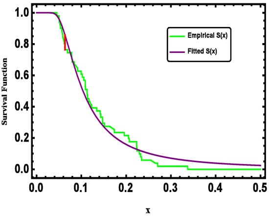
Figure 3.
Empirical and fitted survival function for real data.
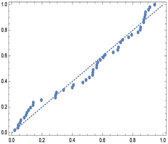
Figure 4.
Probability plot for real data.
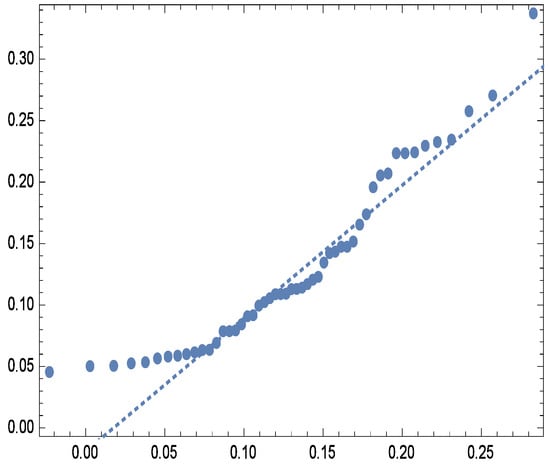
Figure 5.
Quantile plot for real data.
Additionally, Figure 6, Figure 7 and Figure 8 depict the histogram, smoothed histogram, and box-and-whisker plot of the real data, respectively. Figure 9, Figure 10 and Figure 11 illustrate the profile log-likelihood function and contour plot for the parameters and , confirming that it attains a unique maximum, further validating the model’s fit.
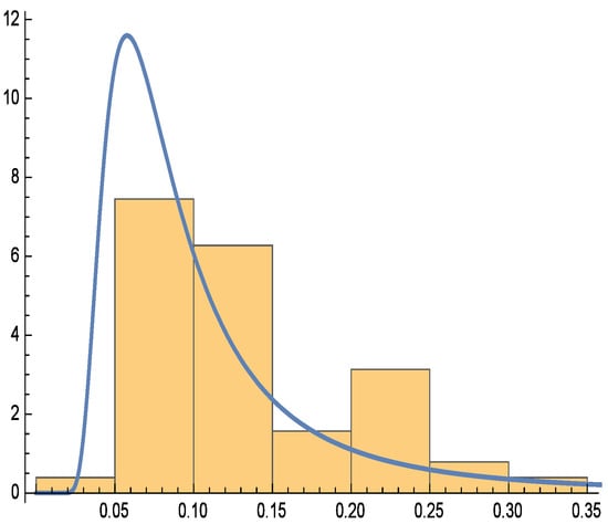
Figure 6.
Histogram for real data.
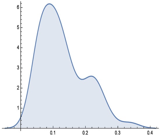
Figure 7.
Smooth histogram for real data.
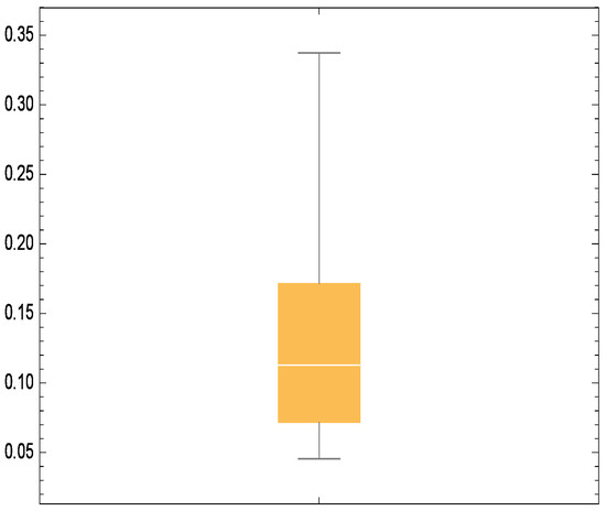
Figure 8.
Box whisker chart for real data.
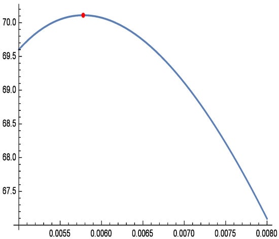
Figure 9.
Profile log-likelihood function of for real data.
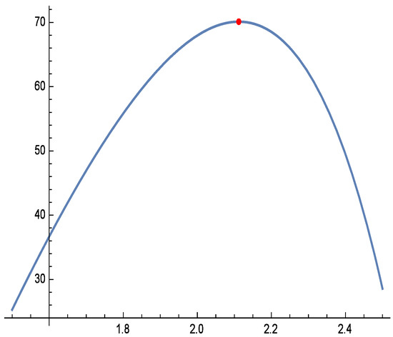
Figure 10.
Profile log-likelihood function of for real data.
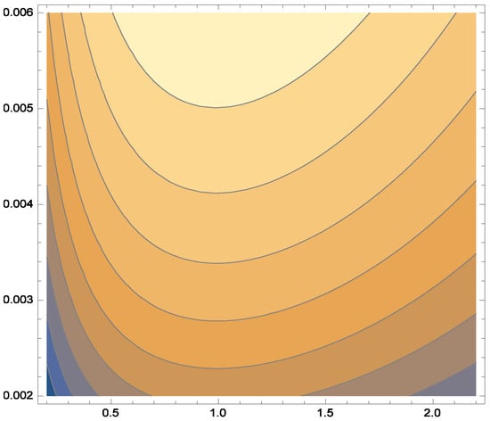
Figure 11.
Contour plot log-likelihood function.
These tests capture different aspects of goodness-of-fit. The K–S test focuses on maximum deviation, the Anderson–Darling test gives more weight to tail discrepancies, and the Cramér–von Mises test assesses integrated squared error across the distribution. Using all three allows for a more comprehensive validation of the model fit.
We analyze the case where censoring is applied to the data. From the dataset, we generate six artificially constructed UHCD sets, as shown in Table 4. We calculate and present frequentist and Bayesian estimates for the parameters , , the survival function , and the hazard function at time , using initial values and . These results are displayed in Table 5, Table 6, Table 7 and Table 8, derived from the dataset in Table 4. Additionally, Table 9, Table 10, Table 11 and Table 12 provide the interval lengths for the 95% two-sided ACI and CRI estimates.
Table 4.
Cases of UHCD.
Table 5.
The Classical estimate and Bayes estimate methods for the parameter .
Table 6.
The Classical estimate and Bayes estimate methods for the parameter .
Table 7.
The Classical estimate and Bayes estimate methods for the .
Table 8.
95% CI and 95% CRI for the .
Table 9.
95% CI and 95% CRI for for real data.
Table 10.
95% CI and 95% CRI for for real data.
Table 11.
95% CI and 95% CRI for for real data.
Table 12.
95% CI and 95% CRI for for real data.
Due to the absence of prior data for the G-IID parameters (, , , and ), the Bayesian analysis relies on non-informative priors under the SE, LINEX, and GE loss functions. To mitigate the influence of initial values, we apply a burn-in period of 3000 iterations from a total of 16,000 MCMC samples, following the algorithm detailed in Section 3. The initial guesses for and are based on their frequentist estimates.
6. Simulation Study Analysis
This section presents the results of a simulation study to support the theoretical conclusions discussed earlier. The study evaluates the performance of the proposed estimators obtained through MLE and Bayesian methods. We estimate the parameters, reliability function, and hazard rate function of G-IID under UHCS. A Monte Carlo simulation was conducted using Mathematica version 10. We compare the point estimators for the lifetime parameters based on MSEs. We also compare the average confidence lengths, where a smaller width indicates better interval estimate performance. We specifically focus on intervals derived from the distribution of the MLEs and the CRIs. The MSE is calculated by
The simulation was conducted by setting different values for r, k, and T, while fixing and for all cases. A total of 18,000 UHC samples were generated from the G-IID, with the first 4000 samples discarded as burn-in. MLEs were used to estimate , , , and , with results presented in Table 13, Table 14, Table 15 and Table 16. The corresponding 95% ACIs are provided in Table 17, Table 18, Table 19 and Table 20. Bayesian estimates were obtained using three loss functions (SE, LINEX, and GE) under an informative prior, with hyperparameters and for . Table 13, Table 14, Table 15 and Table 16 display the Bayesian estimates and the associated MSEs. The 95% CRIs are listed in Table 17, Table 18, Table 19 and Table 20.
Table 13.
The estimated values of under various censoring schemes are presented, with their means and (MSEs) highlighted in bold.
Table 14.
The estimated values of under various censoring schemes are presented, with their means and MSEs highlighted in bold.
Table 15.
The estimated values of under various censoring schemes are presented, with their means and MSEs highlighted in bold.
Table 16.
The estimated values of under various censoring schemes are presented, with their means and MSEs highlighted in bold.
Table 17.
95% CI and 95% CRI for .
Table 18.
95% CI and 95% CRI for .
Table 19.
95% CI and 95% CRI for .
Table 20.
95% CI and 95% CRI for .
Figure 12, Figure 13, Figure 14 and Figure 15 present the MCMC trace plots of the posterior samples for the unknown parameters, as well as for the survival function and hazard function . These plots are used to evaluate the convergence and mixing behavior of the MCMC algorithm.
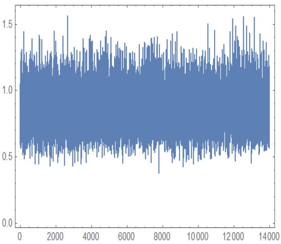
Figure 12.
Trace plot for generated by MCMC.
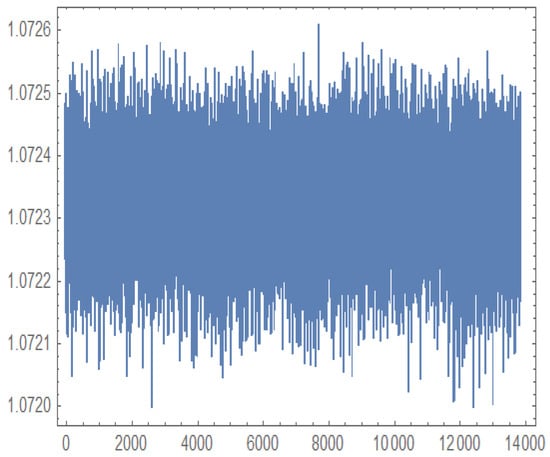
Figure 13.
Trace plot for generated by MCMC.
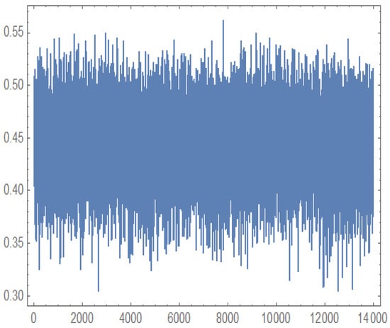
Figure 14.
Trace plot for generated by MCMC.

Figure 15.
Trace plot for generated by MCMC.
7. Conclusions
The methods developed in this paper are directly relevant to the Special Issue theme, particularly in the context of data-driven modeling under censoring and uncertainty using real-life data. This study investigated the estimation of the parameters, reliability function, and hazard function of the G-IID under UHCS. Both classical and Bayesian estimation methods were considered. Bayesian estimates were obtained under three different loss functions: SE, LINEX, and GE. A Monte Carlo simulation study was conducted to evaluate and compare the performance of the proposed estimators.
Several important conclusions can be drawn from the findings:
- Bayesian estimation methods produce significantly narrower CRIs compared to the classical asymptotic confidence intervals, indicating that Bayesian techniques provide higher precision in parameter estimation.
- Bayesian estimates based on the GE loss function consistently achieve the lowest MSE values when compared to those based on SE and LINEX loss functions. This demonstrates the superior performance of the GE-based Bayesian approach, particularly in terms of efficiency and robustness.
- Increasing the values of the censoring parameters r and k leads to a noticeable decrease in the MSEs for the estimates of , , , and . This highlights the importance of larger observed sample sizes in improving estimation accuracy.
- Bayesian estimators outperform maximum likelihood estimators across all scenarios analyzed. They produce smaller MSEs for both the parameters and the reliability-related functions. This confirms the advantages of incorporating prior information and a loss function framework in the estimation process.
- The CRIs resulting from Bayesian methods are not only narrower but also more stable across different censoring schemes. This reliability enhances the confidence in Bayesian interval estimation, especially in highly censored or small sample environments.
- The simulation study revealed that while both classical and Bayesian methods benefit from larger sample sizes, Bayesian methods show a stronger and more consistent improvement in estimation accuracy.
- Under extreme censoring conditions, where traditional methods tend to suffer from large variances and unstable behavior, Bayesian estimation maintains reliable and consistent performance, reinforcing its applicability in practical situations involving incomplete data.
- Among the three loss functions considered, the GE loss function proved to be the most efficient, yielding the smallest MSEs in almost all scenarios.
- Overall, the simulation results strongly support the use of Bayesian estimation techniques, particularly under the GE loss function, when analyzing lifetime data modeled by the G-IID under unified hybrid censoring schemes.
The estimated reliability function and hazard function provide critical insights into the dynamics of COVID-19 mortality. Understanding these functions can help public health officials and researchers make informed decisions regarding interventions and resource allocation. The reliability function represents the probability that an individual survives beyond time t. In the context of COVID-19, it indicates the likelihood of survival for patients diagnosed with the virus over time.
Epidemiological Meaning: A higher value at a given time indicates better survival rates, suggesting effective treatment protocols or lower virulence of the virus.
Monitoring changes in over time can help assess the impact of public health measures, such as vaccination campaigns or social distancing, on mortality rates.
If decreases significantly, it may signal the emergence of more severe variants or the need for updated treatment strategies.
The hazard function quantifies the instantaneous risk of death at time t given that the individual has survived up to that time. It reflects the rate at which deaths occur among the population at risk.
Epidemiological Meaning:
A higher indicates an increased risk of mortality, which can inform healthcare providers about the urgency of care needed for patients at different stages of the disease.
Analyzing can help identify critical time points when patients are most vulnerable, guiding the timing of interventions.
Changes in can also reflect the effectiveness of public health responses, such as the introduction of new treatments or changes in healthcare capacity.
Author Contributions
Conceptualization, M.M.H.; Methodology, M.M.H. and M.M.A.; Software, M.M.H.; Validation, M.M.A. and K.A.A.-K.; Formal analysis, M.M.A.; Investigation, M.M.A.; Resources, K.A.A.-K.; Data curation, K.A.A.-K.; Writing—original draft, M.M.H.; Writing—review and editing, M.M.H.; Visualization, K.A.A.-K.; Funding acquisition, M.M.A. All authors have read and agreed to the published version of the manuscript.
Funding
This work was supported and funded by the Deanship of Scientific Research at Imam Mohammad Ibn Saud Islamic University (IMSIU) (grant number IMSIU-DDRSP2503).
Institutional Review Board Statement
Not applicable.
Informed Consent Statement
Not applicable.
Data Availability Statement
All datasets are reported within the article.
Acknowledgments
The authors extend their appreciation to Deanship of Scientific Research at Imam Mohammad Ibn Saud Islamic University (IMSIU) for funding this work through Research Group: IMSIU-DDRSP2503.
Conflicts of Interest
The authors declare no conflicts of interest.
References
- Epstein, B. Truncated life tests in the exponential case. Ann. Math. Stat. 1954, 25, 555–564. [Google Scholar] [CrossRef]
- Childs, A.; Chandrasekar, B.; Balakrishnan, N.; Kundu, D. Exact likelihood inference based on Type-I and Type-II hybrid censored samples from the exponential distribution. Ann. Inst. Stat. Math. 2003, 55, 319–330. [Google Scholar] [CrossRef]
- Chandrasekar, B.; Childs, A.; Balakrishnan, N. Exact likelihood inference for the exponential distribution under generalized Type-I and Type-II hybrid censoring. Nav. Res. Logist. (NRL) 2004, 51, 994–1004. [Google Scholar] [CrossRef]
- Balakrishnan, N.; Rasouli, A.; Farsipour, N.S. Exact likelihood inference based on an unified hybrid censored sample from the exponential distribution. J. Stat. Comput. Simul. 2008, 78, 475–488. [Google Scholar] [CrossRef]
- Jeon, Y.E.; Kang, S.-B. Estimation of the Rayleigh Distribution under Unified Hybrid Censoring. Austrian J. Stat. 2021, 50, 59–73. [Google Scholar] [CrossRef]
- Yaghoobzadeh Shahrastani, S.; Makhdoom, I. Estimating E-Bayesian of Parameters of Inverse Weibull Distribution Using an Unified Hybrid Censoring Scheme. Pak. J. Stat. Oper. Res. 2021, 17, 113–122. [Google Scholar] [CrossRef]
- Panahi, H.; Lone, S.A. Estimation procedures for partially accelerated life test model based on unified hybrid censored sample from the Gompertz distribution. Eksploatacja Niezawodnosc—Maint. Reliab. 2022, 24, 427–436. [Google Scholar] [CrossRef]
- Seong, Y.; Lee, K. Exact Likelihood Inference for Parameter of Exponential Distribution under Combined Generalized Progressive Hybrid Censoring Scheme. Symmetry 2022, 14, 1764. [Google Scholar] [CrossRef]
- Dutta, S.; Kayal, S. Bayesian and non-Bayesian inference of Weibull lifetime model based on partially observed competing risks data under unified hybrid censoring scheme. Qual. Reliab. Eng. Int. 2022, 38, 3867–3891. [Google Scholar] [CrossRef]
- Dutta, S.; Lio, Y.; Kayal, S. Parametric inferences using dependent competing risks data with partially observed failure causes from MOBK distribution under unified hybrid censoring. J. Stat. Comput. Simul. 2023, 94, 376–399. [Google Scholar] [CrossRef]
- Hasaballah, M.M.; Al-Babtain, A.A.; Hossain, M.M.; Bakr, M.E. Theoretical Aspects for Bayesian Predictions Based on Three-Parameter Burr-XII Distribution and Its Applications in Climatic Data. Symmetry 2023, 15, 1552. [Google Scholar] [CrossRef]
- Hasaballah, M.M.; Tashkandy, Y.A.; Balogun, O.S.; Bakr, M.E. Statistical Inference of Unified Hybrid Censoring Scheme for Generalized Inverted Exponential Distribution with Application to COVID-19 Data. AIP Adv. 2024, 14, 045111. [Google Scholar] [CrossRef]
- Gumbel, E. Statistics of Extremes; Columbia University Press: New York, NY, USA, 1958. [Google Scholar]
- Mousa, M.A.; Jaheen, Z.; Ahmad, A. Bayesian estimation, prediction and characterization for the Gumbel model based on records. Stat. J. Theor. Appl. Stat. 2002, 36, 65–74. [Google Scholar] [CrossRef]
- Nadarajah, S.; Kotz, S. The beta Gumbel distribution. Math. Probl. Eng. 2004, 2004, 323–332. [Google Scholar] [CrossRef]
- Miladinovic, B.; Tsokos, C.P. Ordinary, Bayes, empirical Bayes, and non-parametric reliability analysis for the modified Gumbel failure model. Nonlinear Anal. Theory Methods Appl. 2009, 71, e1426–e1436. [Google Scholar] [CrossRef]
- Feroze, N.; Aslam, M. Bayesian Analysis Of Gumbel Type II Distribution Under Doubly Censored Samples Using Different Loss Functions. Casp. J. Appl. Sci. Res. 2012, 1, 26–43. [Google Scholar]
- Abbas, K.; Fu, J.; Tang, Y. Bayesian estimation of Gumbel type-II distribution. Data Sci. J. 2013, 12, 33–46. [Google Scholar] [CrossRef]
- Feroze, N.; Aslam, M. Bayesian estimation of twocomponent mixture of gumbel type II distribution under informative priors. Int. J. Adv. Sci. Technol. 2013, 53, 11–30. [Google Scholar]
- Reyad, H.M.; Ahmed, S.O. E-Bayesian analysis of the Gumbel type-II distribution under type-II censored scheme. Int. J. Adv. Math. Sci. 2015, 3, 108–120. [Google Scholar] [CrossRef]
- Sindhu, T.N.; Feroze, N.; Aslam, M. Study of the left censored data from the gumbel type II distribution under a bayesian approach. J. Mod. Appl. Stat. Methods 2016, 15, 10–31. [Google Scholar] [CrossRef]
- Abbas, K.; Hussain, Z.; Rashid, N.; Ali, A.; Taj, M.; Khan, S.A.; Manzoor, S.; Khalil, U.; Khan, D.M. Bayesian estimation of gumbel type-II distribution under type-II censoring with medical applicatioNs. Comput. Math. Methods Med. 2020, 2020, 1876073. [Google Scholar] [CrossRef]
- Qiu, Y.; Gui, W. Statistical Inference for Two Gumbel Type-II Distributions under Joint Type-II Censoring Scheme. Axioms 2023, 12, 572. [Google Scholar] [CrossRef]
- Cohen, A.C. Maximum likelihood estimation in the Weibull distribution based on complete and on censored samples. Technometrics 1965, 5, 579–588. [Google Scholar] [CrossRef]
- Greene, W.H. Econometric Analysis, 4th ed.; Prentice Hall: New York, NY, USA, 2000. [Google Scholar]
- Almetwally, E.M. Application of COVID-19 pandemic by using odd lomax-G inverse Weibull distribution. Math. Sci. Lett. 2021, 10, 47–57. [Google Scholar]
Disclaimer/Publisher’s Note: The statements, opinions and data contained in all publications are solely those of the individual author(s) and contributor(s) and not of MDPI and/or the editor(s). MDPI and/or the editor(s) disclaim responsibility for any injury to people or property resulting from any ideas, methods, instructions or products referred to in the content. |
© 2025 by the authors. Licensee MDPI, Basel, Switzerland. This article is an open access article distributed under the terms and conditions of the Creative Commons Attribution (CC BY) license (https://creativecommons.org/licenses/by/4.0/).