Article

Diversity and Semiconvergents in Pythagorean Tuning

Departament de Matemàtiques, Universitat Politècnica de Catalunya, 08028 Barcelona, Spain
Axioms 2025, 14(6), 471; https://doi.org/10.3390/axioms14060471
Submission received: 12 May 2025 / Revised: 9 June 2025 / Accepted: 11 June 2025 / Published: 17 June 2025
(This article belongs to the Special Issue Applied Mathematics and Numerical Analysis: Theory and Applications)

Abstract

:
Several approaches to building generalized Pythagorean scales provide interpretation for the rational approximation of an irrational number. Generally, attention is paid to the convergents of the continued fraction expansions. The present paper focuses on the sequences of semiconvergents corresponding to the alternating best one-sided approximations. These sequences are interpreted as scale lineages organized as a kinship. Their properties are studied in terms of the two types of tones and elementary intervals, since each scale contains the tones of the previous scale plus the newly added tones, i.e., the generic diatones and accidentals. For the last scale of a lineage, the octave is regularly subdivided by sections, separated by a single elementary interval of the other type. Lineages are therefore related to the scale diversity with regard to their generic diatones and accidentals, which is analyzed from the Shannon diversity index, either for tone abundance or interval occupancy.

Graphical Abstract

1. Introduction

Pythagorean tuning is a musical example of a rational approximation of an irrational number, the generator tone. A scale tone  ν k , k Z , is an iterate of the third harmonic of a fundamental frequency ν 0 (generally assumed as ν 0 = 1 ), ν k = 3 k ν 0 , reduced to the range of frequencies of one octave [ 1 , 2 ) . In the logarithmic space of the frequencies, the scale notes are x k = log 2 ν k = k log 2 3 [ k log 2 3 ] , i.e., the iterate minus its integer part (the integer part of a R is the floor function a if a 0 and the ceiling function a if a < 0 ). Sometimes, it is useful to use backward iterates ( k < 0 ) in order to obtain tones as close as possible to simple ratios [1], such as considering the class of the fifth harmonic 5 4 3 8 2 13 instead of 5 4 3 4 2 6 . The scale notes can be represented clockwise in the circle of the octave S 0 = R / Z (i.e., the interval [ 0 , 1 ) by identifying its endpoints, 0 representing the fundamental) and multiplied by 1200 to give their value in cents (¢).
Several mathematical approaches have been used to determine the number of tones of a well-formed scale [2,3,4], which will be reviewed in the next section. These approaches are also valid when the generator tone ( g = 3 , for Pythagorean scales, although the scale can be interpreted as generated from the iterations of the third harmonic of the fundamental projected onto the octave or by its class 3 2 , i.e., the fifth.) is any positive real number, which is known as generalized Pythagorean tuning. Depending on the approach and on the number of generators, well-formed scales have also been referred to with different names, such as moments of symmetry [5,6], gammes naturelles (in French) [7,8], etc. Here, by following [9,10], a monogenous well-formed scale with one generator g > 0 will be referred to as a cyclic scale to simplify.
These mathematical approaches include several areas of numerical analysis, such as iterative methods [11,12], continued fraction approximations [13], Farey sums, the Stern–Brocot tree and its dual, the Raney tree [14,15] or Calkin–Wilf tree [16,17], mechanical or Sturmian words [18,19,20], entropy and interval regularity [21,22,23,24,25], etc. Depending on whether we are focusing on the scale tones, their indices, their geometry, their intervals, etc., it is convenient to take into account one or several of these approaches.
A fundamental property of cyclic scales is that the partition of the octave induced by the scale notes has exactly two sizes of scale steps, and each number of generic intervals occurs in two different sizes, which is known as Myhill’s property [26,27]. In addition, the two elementary intervals are associated with two families of tones, the generic diatones and accidentals [10]. Relying on their relative abundance, i.e., the proportion between the number of diatones and accidentals and their occupancy, i.e., the fraction of octave they occupy, the scales may show different properties, such as having more degrees of rotational symmetry for some specific intervals, ranging a wider part of the octave subdivided into regular intervals, both types of tones being well mixed or forming lumps, etc. Depending on the musical context, both kinds of diversity, for abundance and occupancy, are properties to evaluate.
In the current paper, scale diversity is studied by using the Shannon index based on entropy, and it is analyzed how this is related to the sequences of the best one-sided rational approximations of the generator tone.
The next sections are organized as follows. In Section 2, several approaches explain how Pythagorean scales are built, being equivalent to computing the canonic continued fraction expansions of the generator. An iterative algorithm for determining the chain of cyclic scales is used to introduce the key indices that characterize a scale, namely the indices of the extreme tones m , M and the scale digit δ . They will be related to the new concepts of ruling index and the lineage of scales.
Section 3 pays attention to the lineages and both types of tones and intervals by enumerating their properties and pointing out their relationship to the semiconvergents of the canonic continued fraction expansions of the generator.
Section 4 introduces the diversity indices, either for abundance h or occupancy h, and derives their main properties when applied to cyclic scales.
Section 5 describes the behavior of h and h in terms of the key indices of the cyclic scales. In particular, conditions for increasing or decreasing trends of the abundance and occupancy diversity indices along lineages are analyzed.
The relationship between the diversity indices and the partition entropy of the scale is provided in Section 6.
Section 7 summarizes the conclusions and applies the previous results to describe the first lineages in Pythagorean tuning.

2. Generalized Pythagorean Tuning

2.1. A Geometric Approach

Without loss of generality, we can assume the note iterates as x k for k 0 , beginning with a certain x 0 . Notice that to start the iterates with a negative value, say k = 2 with fundamental x 0 = 0 , would be equivalent to the iterates x k starting at k = 0 with fundamental x 0 = x 2 . The number tones of an n-tone cyclic scale E n g is determined when the distance from x 0 to x n in the circle S 0 is lower than the distance to the iterates x k , with 0 < k < n , either by one side or by both sides, which is known as a closure condition [2,3,4]. Then, x n is identified with x 0 , by providing the scale with an algebraic structure of the factor group [7].
By following the notation in [9,10], when the scale tones other than the fundamental
ν k = g k 2 k ; k = [ k log 2 g ] ; k = 1 , , n 1
are ordered from lowest to highest pitch (say, in cyclic order or by ordinal) there are two extreme tones, the minimum tone  ν m and the maximum tone ν M , which determine the two elementary factors in the multiplicative space of frequencies, namely U ν m = g m 2 m (up the fundamental) and D 2 ν M = 2 M + 1 g M (down the fundamental), so that U M D m = 2 . For n 2 , the indices satisfy n = m + M , all of them coprime. These factors have the corresponding elementary intervals in the additive logarithmic space of notes, u = log 2 U and d = log 2 D , with M u + m d = 1 .
The tone ν n = g n 2 n , which does not belong to the scale E n g , provides the closure condition, either ν n 1 + , above the fundamental, or ν n 2 , below the fundamental.
Two parameters can be used to know whether ν n closes above or below the fundamental. For m , M 0 , and by using the index N = m + M + 1 (also N = [ n log 2 g + 1 2 ] ), the parameters are the scale closure, γ n = g n 2 N , which is a value close to 1, and the scale digit, δ = N n , which takes values 0 or 1. Thus, δ = 0 γ n > 1 ( ν n 1 + ) and δ = 1 γ n < 1 ( ν n 2 ). The scale closure also satisfies γ n = U D , so that its value depends on the relative size of the elementary factors.

2.2. Best and Good Rational Approximations of log 2 g

The above approach can be interpreted as N n being a convergent or semiconvergent of the canonic continued fraction expansion of log 2 g .
The scales corresponding to the best rational approximations (best approximation of the second kind [28,29]) N n of log 2 g are the convergents of its canonic continued fraction expansions (Best Approximation Theorem (e.g., [30])). However, while the convergents are the best double-sided approximations, the semiconvergents are only the best one-sided approximations.
The quotient of indices N n is a best approximation of log 2 g if one of the following cases takes place [9]:
(i)
If δ = 0 , then 1 < ν n < 2 ν M < ν m , and
0 < n log 2 g N < M log 2 g ( M + 1 ) < m log 2 g m
(ii)
If δ = 1 , then ν M 2 < 1 ν m < ν n 2 < 1 , and
0 < n log 2 g N < m log 2 g m < M log 2 g ( M + 1 )
The best approximations are associated with the best closure γ n 1 . They provide optimal scales. Then, by considering the interval closure  ϕ n = log 2 γ n in S 0 ,
E n g is optimal | ϕ n | < | ϕ k | , 0 < k < n
On the other hand, the good rational approximations (best approximation of the first kind) are the convergents and some semiconvergents of the canonic continued fraction expansions. They generate accurate scales [23] and are associated with the best estimations of the generator 2 N n g .
The set of best one-sided approximations is equal to the set of good one-sided approximations [29] (Theorem 4.5). Therefore, both convergents and semiconvergents of the canonic continued fraction expansions of log 2 g are good one-sided approximations, according to one of these cases:
(i)
If δ = 0 , then 1 < ν n < ν m , and
k k m m < N n < log 2 g , 0 < k < n
That is, the closure above the fundamental means a left-sided approximation to log 2 g .
(ii)
If δ = 1 , then ν M 2 < ν n 2 < 1 , and
log 2 g < N n < M + 1 M k + 1 k , 0 < k < n
The closure below the fundamental means a right-sided approximation to log 2 g + .

2.3. Iterations in Terms of the Indices m, M, and δ

Cyclic scales (whether optimal or not) form a chain, E n g E n + g In each link, the scale E n + g is composed of the tones of E n g , the generic diatones, in addition to the new non-adjacent tones, the generic accidentals [10].
Based on the above approaches, cyclic scales can also be obtained from the following iterative process. Starting from the indices of the extreme tones m and M of E n g , with n = m + M ( n 2 ), for the next cyclic scale in the chain E n + g , these values are obtained as:
( i ) m + = m + M , M + = M , n + = n + M δ = 0 ( ii ) m + = m , M + = m + M , n + = n + m δ = 1
Therefore, according to (1), one of the indices of the extreme tones always repeats. This happens while approximations are improving by one side, until reaching an optimal scale, then the approximations begin to improve by the other side.
It is worth mentioning the following theorem [9] (Theorem 5.1).
Theorem 1.
In the link E n g E n + g , δ δ + E n g is optimal.
Definition 1.
If R is the index of one of the extreme tones, all the scales sharing this index form the R-lineage (or, simply, lineage), and each scale represents a stage of the lineage. From the first repetition of R (second stage of a lineage) until the end of the lineage, R is the ruling index.
Table 1 displays the lineages for the first non-trivial Pythagorean scales ( g = 3 ) in terms of their i-th ordinal. It is built according to the following algorithm and initial conditions, by assuming the null scale E n 0 3 with n 0 = 0 , and the trivial scale E n 1 3 with n 1 = 1 , which is composed of the fundamental tone alone. Obviously, the first non-trivial scale E n 2 3 with n 2 = 2 , is formed by the class of the generator tone in addition to the fundamental, from which the others are generated:
m 2 = 1 ; M 2 = 1 ; n 2 = 2 ; δ 1 = 0 for i = 3 to 51 do if δ i 1 = 0 then m i = n i 1 ; M i = M i 1 ; n i = n i 1 + M i ; δ i = m i + M i + 1 n i ; R i = M i else m i = m i 1 ; M i = n i 1 ; n i = n i 1 + m i ; δ i = m i + M i + 1 n i ; R i = m i end if end for
The lineages may be noted as 3 5 7 , 7 12 17 , 17 29 41 53 , 53 94 , etc. From the foregoing code, by defining R 1 1 , it is straightforward to see the following.
Lemma 1.
For i 2 , R i R i 1 and
(a) 
n i = n i 1 + R i .
(b) 
n i = k = 1 i R k .
(c) 
n k is the first of a lineage ⇔ R k + 1 = n k 1 and R k + 1 R k .
(d) 
In the R i -lineage, if n k is the first of the lineage ( k < i 1 ), then n i = n k + ( i k ) R i .
(e) 
n k is the first of a lineage ⇔ δ k 1 δ k
Therefore, owing to item (e), we reformulate Theorem 1,
Theorem 2.
E n k g is the first of a lineage ⇔ E n k 1 g is optimal.
And, owing to item (c),
Corollary 1.
The number of tones of each optimal scale is the ruling index of a lineage.

2.4. Mechanical Words

The procedure to determine cyclic scales and their refinements is also related to the concept of mechanical or Sturmian words used in several approaches to the theory of well-formed scales and modes [18,19,20], which are based on methods of combinatorics on words (e.g., [31]).
A cyclic scale can be defined as a Christoffel word of the alphabet { U , D } , associated with both elementary factors, with slope m M and length n. The octave is then represented by a word with M letters U and m letters D since U M D m = 2 . For cyclic scales, the first step of the octave must be U and the last step must be D. Each value n is associated with one word w n , for instance, w 2 = U D , w 7 = U U U D U U D , w 12 = U D U D U D D U D U D D .
Depending on the relative size of the elementary factors, the scale E n g can be refined to form the next cyclic scale E n + g in the following way: if U < D , by factorizing D = U D + , otherwise by factorizing U = U + D , and so on.
It is important to remark the following properties [10] used in the next section:
  • If m > M the generic accidentals are the tones obtained by increasing the previous one by a factor U, and come alone. Then, U is the accidental factor and D the diatonic factor.
  • If M > m , the generic accidentals are the tones that are followed by a factor D and come alone. Then, D is the accidental factor, and U is the diatonic factor.
  • In a scale, the relative size of the elementary factors relies on sign ( ϕ n ) (or δ ) and the role diatone/accidental relies on sign ( m M ) ; therefore, in E n g , they are not related (in the link E n g E n + g , sign ( m + M + ) depends on sign ( ϕ n ) instead of sign ( ϕ n + ) ).
  • Consecutive optimal scales have alternate short and long elementary factors.
To better understand how the mechanical words are formed, we examine two examples, namely the successive cyclic scales E 5 3 E 7 3 and E 7 3 E 12 3 .
For n = 5 , the indices of the extreme tones are m = 2 , M = 3 , and the associated word is w 5 = U U D U D . The next cyclic scale is for n + = 7 , where its first five iterates (its generic diatones) are the tones of the 5-tone scale. The indices of the extreme tones are m + = 2 , M + = 5 , with M + > m + . The index of the minimum tone and its associated factor U are maintained. Therefore, in the 5-tone scale, the interval factorized to form the next scale is the one associated with the maximum tone, D = U D + . Hence, the new tones of the 7-tone scale, i.e., its accidentals, are placed just at the beginning of a factor D + , and the generic diatones, just at the beginning of a factor U (note that the factors U are maintained and the factors D + come alone). Thus, w 7 = U U ( U D + ) U ( U D + ) . Remark that, in the 5-tone scale, the relative size of the elementary factors is U D < 1 . Since it is an optimal scale, in the next scale, this relationship will change according to U D + > 1 so that the next letter to be split will be U.
Now, we take as reference the 7-tone scale, with associated word w 7 = U U U D U U D . The next cyclic scale is for n + = 12 , where the first seven iterates (its generic diatones) are the tones of the 7-tone scale. The new indices of the extreme tones are m + = 7 , M + = 5 , with m + > M + . The index of the maximum tone is maintained, and so is the factor D. Therefore, in the 7-tone scale, the interval factorized is the one associated with the minimum tone, U = U + D . Then, the generic accidentals of the 12-tone scale come just at the end of a factor U + (which come alone), and the generic diatones come at the end of a factor D. Thus, w 12 = ( U + D ) ( U + D ) ( U + D ) D ( U + D ) ( U + D ) D . Since the 7-tone scale is not optimal, in the next 12-tone scale, the relationship U D > 1 is still maintained, U D + > 1 , so that the next letter to be split will also be U.

3. Lineages

3.1. Diatonic and Accidental Intervals Along Lineages

The approach from mechanical words allows us to understand easily how the elementary intervals are subdivided along lineages. In this case, it is easier to describe the process in the space of notes instead of frequencies. Note that this is an alternative geometric interpretation of the alternating best one-sided rational approximations of an irrational number.
For the i-th cyclic scale, the n i notes divide the octave S 0 into n i intervals (which are represented horizontally in Figure 1). These intervals are a mixture of both elementary intervals of different sizes, u i and d i so that M i u i + m i d i = 1 . The first interval is always u i and the last is d i . The next cyclic scale of n i + 1 tones is obtained by dividing the greatest of both intervals u i , d i into two intervals, one with the same size as the smaller interval and the other with the remaining size ( u i always remains on the left and d i on the right). The old notes are the generic diatones, and the new ones are the accidentals. The interval that is maintained, i.e., the smaller one, becomes the diatonic interval in the next scale.
Figure 1 displays the refinement process of the first Pythagorean scales, i.e., n 2 = 2 and the scales of the lineage 3 5 7 , corresponding to the three stages n 3 , n 4 , n 5 , and involving two links. Just before a change of the relative sizes of u and d, the ratio N n is a best approximation of log 2 g , as for n = 2 and 5. Therefore, the smallest interval becomes the unit of measurement along the lineage.
Let us note that, in the last stage, for n 5 = 7 , after two subdivisions of d 3 , between two intervals d 5 , we may have two or three intervals u 5 , i.e., at least the number of links of the lineage and, at most, the number of stages, since the interval u 3 in the scale with n 3 = 3 tones was already the accidental interval, which came alone.

3.2. Number of Generic Diatones and Accidentals Along Lineages

The refinement process during a linage is now detailed in terms of the indices. Let us assume that, in the link E n i g E n i + 1 g , the value of δ i changes. Then, E n i g is optimal, which has the following consequences:
(1)
In E n i + 1 g , the ruling of R i + 1 = n i + 1 n i and the R i + 1 -lineage end and begins the R i + 2 -lineage with R i + 2 = n i .
(2)
In E n i + 2 g , the ruling of R i + 2 = n i begins.
(3)
A particular case occurs when E n i g and E n i + 1 g are two consecutive optimal scales. Then, R i + 2 = n i rules only one stage. In this case, there will be two consecutive beginnings of lineage. We will say the R i + 2 -lineage is short.
(4)
For E n i + 1 g , the number of generic diatones is n i , which is the number of tones of an optimal scale, and the number of accidentals is n i + 1 n i . Hence, n i > n i + 1 n i .
(5)
In the first stage of the ruling index R i + 2 = n i , the number of generic diatones is n i + 1 , and the number of accidentals is n i < n i + 1 .
(6)
While ruling R i + 2 = n i , for the successive j-th scales, the number of generic diatones, n j n i , always increases, and the number of accidentals is constant n i < n j n i .
(7)
In E n i + 2 g , the sign of m i + 2 M i + 2 is opposite to that of m i + 1 M i + 1 and remains constant while ruling R i + 2 .
In other words, if for j > i + 1 , the ruling index is R j = n i , then the first scale of the R j -lineage is E n i + 1 g and sign ( m i + 1 M i + 1 ) = sign ( m i + 2 M i + 2 ) .
(8)
Since an optimal scale E n i g is minimal in | ϕ n i | , if the next scales E n j g , j > i , are not optimal, then | ϕ n j | > | ϕ n i | along the new lineage, until reaching the next optimal scale, which is the penultimate of the lineage.
Definition 2.
Let us consider the lineage, whose first scale is E n i + 1 g . The subdiatones of the lineage are the generic diatones of its first scale, i.e., the number of tones of the optimal scale E n i g , matching the ruling index of the lineage. The superdiatones of the lineage are the generic diatones of its last scale, i.e., the number of tones of its penultimate, optimal scale. All of them are associated with the corresponding subdiatonic and superdiatonic intervals.
Lemma 2.
(a) 
A lineage contains at least one optimal scale, i.e., its penultimate, and at most two optimal scales, i.e., its penultimate and its last one.
(b) 
If the first scale of the lineage is optimal, it is its penultimate. Then the lineage is short.
(c) 
For the last scale of a lineage, the number of generic accidentals is the number of subdiatones of the lineage, and the number of generic diatones is the number of superdiatones, both indices corresponding to the number of tones of the two previous optimal scales.

4. Shannon Diversity Index

In [23], the concept of entropy was used to compare scale partitions and to classify them with regard to the regularity of their intervals. This involved the number of intervals together with their respective size, and it could be applied to cyclic and non-cyclic scales. The bias of a cyclic scale was defined from its partition entropy as θ n = 1 log 2 n ( log 2 n H n ) . It was proven that scales with minimal bias were optimal. In this way, the partition entropy is related to the best rational approximations of the generator.
Entropy can also be applied to compare scales with regard to their composing tones and intervals separately or to determine lineages, which are organized as a kinship. Such an approach, as we have seen, is related to the alternating sides of the semiconvergents of the canonic continued fraction expansions of the generator.
A cyclic scale is composed of two populations, either for tones or intervals, associated with the generic diatones and accidentals. Regardless of how the tones or intervals are mixed, the proportion in which they are present—either in abundance or in the space the intervals occupy the octave—determines some kind of diversity that may have consequences in music.
There are several indices to quantify diversity. Here, we focus on the Shannon diversity index based on entropy [32]. The original purpose of Shannon’s index was to determine the uncertainty in predicting the following letter of a given alphabet in a given string. Thus, the more letters there are, the more difficult it is to predict which letter will be next in the string. Similarly, the closer their proportional abundances in the string, the more difficult it will also be to predict the next letter.
If S is the cardinality of the alphabet and p i is the proportion of characters belonging to the i-th type of letter in the string, the Shannon index is defined as
H = i = 1 S z ( p i ) ; z ( p i ) = p i log 2 p i
It is useful to remember the following three properties of the z function, which will simplify the forthcoming operations:
z a b + z 1 a b = 1 b z ( a ) z ( b ) + z ( b a ) ; b 0 z ( a b ) = a z ( b ) + b z ( a ) a b log 2 a b = a z ( b ) b z ( a ) ; b 0
For cyclic scales, the number of types of notes and intervals is fixed to S = 2 . What is variable is the proportion between generic diatones and accidentals. Since there are m and M notes and intervals of the respective types, then the whole scale plays the role of the string of the alphabet, with respective proportions p 1 = m n , p 2 = M n . Thus, with regard to abundances, by taking into account (3), we write the diversity index as
h ( E n g ) = z m n + z M n = log 2 n + 1 n z ( m ) + z ( M ) = = log 2 n 1 n m log 2 m + M log 2 M
Depending on the scale, the number of generic diatones is either m or M, always the greatest of both. Hence, the ratio of accidentals to the number of scale notes is always less than 1 2 . These values depend on the scale digit δ . For two consecutive scales E n g E n g , with respective scale digits δ and δ , if δ = 0 , then m = n is the number of generic diatones in E n g , while if δ = 1 , this number is M = n .
In the limiting case m n = M n = 1 2 , then h = 1 , which means that the uncertainty is maximum in predicting the type of one arbitrary scale note.
If we consider the n-tone equal temperament (i.e., regular) scale associated with the cyclic scale E n g , which is a degenerate cyclic scale, it is still possible to distinguish between generic diatones and accidentals (likewise in the piano keys), although their associated intervals are of equal size.
Nevertheless, we must bear in mind that there are other degenerate cases. In terms of the interval closure ϕ n , the respective intervals fill in the octave as
u = 1 + m ϕ n n , d = 1 M ϕ n n ; M u + m d = 1 , ϕ n = u d
Hence, if ϕ n = 0 , then the n-tone scale is regular. However, when considering the equal temperament scales resulting from the degenerate cases u 0 n = m and d 0 n = M , then h = 0 since there would only remain one type of scale tone. However, in such a case, we would not be dealing with an n-tone cyclic scale.

4.1. Abundance–Diversity Index

In the link E n k 1 g E n k g ( k 2 ) of the chain of cyclic scales, the generic diatones are the first n k 1 iterates of E n k g and the accidentals are the last n k n k 1 iterates ( n k n k 1 < n k 1 ). Then, it is useful to write the abundance–diversity index as follows,
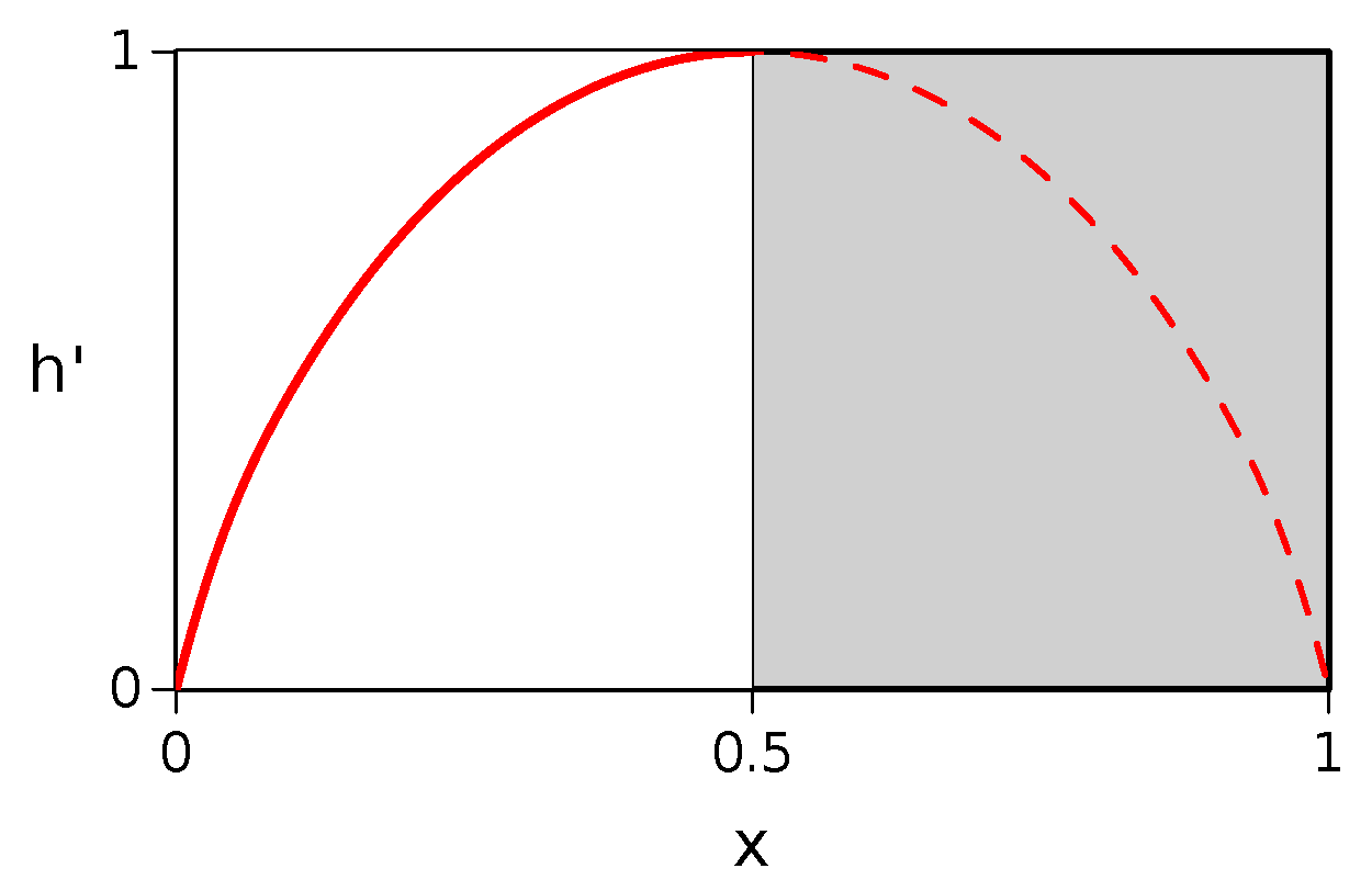
h k h ( E n k ) = z n k n k 1 n k + z n k 1 n k = = log 2 n k + 1 n k z ( n k n k 1 ) + z ( n k 1 ) = = log 2 n k 1 n k ( n k n k 1 ) log 2 ( n k n k 1 ) + n k 1 log 2 n k 1
If n k = n k 1 , obviously h k = 0 . If n k 2 = n k 1 = n k n k 1 , then h k = 1 , although it will always occur that n k n k 1 < n k 2 . Therefore, as shown in Figure 2, in terms of the fraction of accidentals x = n k n k 1 n k ( 0 < x < 1 2 ), the diversity index h ( x ) is an increasing, bijective function h : ( 0 , 1 2 ) ( 0 , 1 ) .
In consequence, since the fraction of accidentals decreases from the second stage of a lineage up to the end (i.e., along an invariant ruling index), the abundance–diversity index also decreases (Lemma 5).
The contribution of the generic accidentals to the whole abundance–diversity index can be evaluated from the accidental-abundance, as
α k α ( E n k ) = 1 h k n k n k 1 n k log 2 n k n k 1 n k ; 0 < α k < 1 2
Similarly, for the generic diatones, the diatone-abundance can be defined as
β k β ( E n k ) = 1 h k n k 1 n k log 2 n k 1 n k ; α k + β k = 1

4.2. Cumulative Abundance–Diversity Index

If instead of focusing on one link of the chain, we take into account all the links up to E n k g , it is also possible to consider the successive accidentals of the partial chain E n 1 g E n k 1 g E n k g , k 2 , as if they were of different types. In this way, the emphasis is placed even more on the generic accidentals of E n k g than on its diatones, since these remain dissolved in the many accidentals of the previous scales to E n k g . According to (2), since n 0 = 0 , the cumulative abundance–diversity index is given by
H k H ( E n k g ) = i = 1 k z n i n i 1 n k
Theorem 3.
The cumulative abundance–diversity index satisfies
H k = i = 1 k n i n k h i
Proof. 
Owing to the sub-additivity property of the entropy, we can evaluate separately the entropy of the partition corresponding to the last link of the chain, E n k 1 g E n k g , and the entropy coming from the remaining subpartitions, so that
H k = z n k n k 1 n k + z n k 1 n k + n k 1 n k H k 1
According to (6), the first two terms on the right-hand side match the index h k , so that
H k = h k + n k 1 n k H k 1
By writing recursively the above expression, we get (3). □
The cumulative abundance–diversity index is upper-bounded
H k k z 1 k = log 2 k
in which the maximum would be attained if n i n i 1 = n k k , i .
The cumulative accidental-abundance of E n k can be expressed as
A k A ( E n k ) = 1 H k n k n k 1 n k log 2 n k n k 1 n k ; 0 < A k < 1 2
The relationship between both accidental-abundance indices is straightforward to obtain by comparing (7) and (8),
α k h k = A k H k
Thus, by taking into account (3), we obtain the following relationship.
Corollary 2.
The accidental-abundance indices satisfy
α k = A k i = 1 k n i n k h i h k

4.3. Occupancy–Diversity Index

The other criterion to distinguish between generic diatones and accidentals is to consider the fraction of the octave that the intervals u and d occupy.
Let us remember that, if m > M , the diatonic interval is d, which ends in a generic diatone. Then, the interval d does not change in the link E n g E n g . Each u-interval ends in an accidental.
Otherwise, if M > m , the diatonic interval is u, which starts in a diatone. The interval u is maintained in this link. Each d-interval starts in an accidental.
For each cyclic scale, we gather all the M u-intervals and the m d-intervals, so that s = M u and 1 s = m d . The occupancy–diversity index is then given by
h ( E n g ) z ( s ) + z ( 1 s ) = z ( M u ) + z ( m d )
By taking into account (5), the index h can be written as follows,
h ( E n g ) = z m ( 1 M ϕ n ) n + z M ( 1 + m ϕ n ) n = = log 2 n + 1 n z m ( 1 M ϕ n ) + z M ( 1 + m ϕ n ) = log 2 n 1 n m ( 1 M ϕ n ) log 2 m ( 1 M ϕ n ) + M ( 1 + m ϕ n ) log 2 M ( 1 + m ϕ n )
Bearing in mind (4), if ϕ n = 0 , we obtain the obvious result for n-tone regular scales,
Lemma 3.
If ϕ n = 0 , then h ( E n g ) = h ( E n g ) = z m n + z M n .
Although the number of accidentals is lower than n 2 , their size is not restricted to less than half an octave since it relies on the sizes of u and d. This means that according to the shape of the entropy of Figure 2, there are two values of s providing the same index value. This is because h depends on ϕ n , while h does not.
For fixed values m , M , the function h can be written in terms of ϕ n 1 m , 1 M as
h ( m , M ; ϕ n ) = h ( m , M ; ξ 0 + ξ ) ; ξ 0 = 1 2 1 M 1 m , 1 2 1 M + 1 m ξ 1 2 1 M + 1 m
Notice that, according to [23] (Equations A4 and A7), u , d > 0 implies 1 m < ϕ n < 1 M . Then, it is also fulfilled 1 m < 1 M 1 m ϕ n < 1 M .
Then, it is immediate to prove the following equalities.
Lemma 4.
(a) 
h ( m , M ; ξ 0 ) = 1 ;
(b) 
h ( m , M ; ξ 0 + ξ ) = h ( m , M ; ξ 0 ξ ) ;
(c) 
h ( m , M ; 0 ) = h ( m , M ; 2 ξ 0 ) .
Therefore,
h ( m , M ; ϕ n ) = h m , M ; 1 M 1 m ϕ n h ( E n g ) = h ( m , M ; 0 ) = h m , M ; 1 M 1 m
In this case, we cannot affirm that the occupancy–diversity index has a monotonous increasing or decreasing trend along the stages of an invariant ruling index. Along a lineage, one of the indices m or M is maintained, and so is the sign of ϕ n , until the penultimate (optimal) scale. Thus, the quantities M u and m d vary, the lower one, the greater the other. We shall see in Section 5.2 that the beginning of a non-short lineage matches a local minimum of h so that between two consecutive non-short lineages, the occupancy–diversity index first increases and afterwards decreases.

5. Diversity Along Lineages

5.1. Local Minima of h

As explained in Section 3.2, item (6), while an index is ruling, the number of accidentals is constant and lower than the number of generic diatones, which increases. Therefore, as proven below, the abundance–diversity index decreases. In the next stage, the first of a new ruling index, according to item (7), there is a change of role diatones/accidentals between indices.
To analyze the trend of the abundance–diversity index during the stages of a ruling index, we define the function
ζ ( x ) = z ( x ) + z ( 1 x ) , x [ 0 , 1 ]
It is concave and satisfies ζ ( 0 ) = ζ ( 1 ) = 0 , is symmetric about 1 2 , and has a maximum ζ ( 1 2 ) = 1 . By choosing x = min ( m n , M n ) , then x 1 2 . Hence, it is fulfilled
x < x ζ ( x ) < ζ ( x ) ; x , x 0 , 1 2
That is, in [ 0 , 1 2 ] the function ζ is bijective and increases, so that to check whether ζ ( x ) < ζ ( x ) it is equivalent to checking whether x < x . We express (4), for the i-th stage, as
h i = ζ ( x i ) ; x i = min m i n i , M i n i
According to (1), changes from h i to h i + 1 depend on the values δ i 1 and δ i , and do not depend on δ i + 1 . We study the following cases:
(1)
If δ i 1 = 0 , δ i = 0 , then
m i = m i 1 + M i 1 ; M i = M i 1 ; M i < m i ; h i = ζ M i m i + M i ; m i + 1 = m i + M i ; M i + 1 = M i ; M i + 1 < m i + 1 ; h i + 1 = ζ M i m i + 2 M i .
Therefore, h i > h i + 1 (noted as h ).
(2)
If δ i 1 = 1 , δ i = 0 , then
m i = m i 1 ; M i = m i 1 + M i 1 ; m i < M i ; h i = ζ m i m i + M i ; m i + 1 = m i + M i ; M i + 1 = M i ; M i + 1 < m i + 1 ; h i + 1 = ζ M i m i + 2 M i .
Whether h increases or decreases depends on whether m i m i + M i is lower or greater than M i m i + 2 M i . By noting r i = m i M i , it is straightforward to see that
(a)
If 0 < r i < 1 + 5 2 , then h i < h i + 1 ( h ).
(b)
If 1 + 5 2 < r i < 1 , then h i > h i + 1 ( h ).
(3)
If δ i 1 = 0 , δ i = 1 , then
m i = m i 1 + M i 1 ; M i = M i 1 ; M i < m i ; h i = ζ M i m i + M i ; m i + 1 = m i ; M i + 1 = m i + M i ; m i + 1 < M i + 1 ; h i + 1 = ζ m i 2 m i + M i .
Whether h increases or decreases depends on whether M i m i + M i is lower or greater than m i 2 m i + M i . As in the previous case, it is straightforward to see that
(a)
If 1 < r i < 1 + 5 2 , then h i > h i + 1 ( h ).
(b)
If 1 + 5 2 < r i , then h i < h i + 1 ( h ).
(4)
If δ i 1 = 1 , δ i = 1 , then
m i = m i 1 ; M i = m i 1 + M i 1 ; m i < M i ; h i = ζ m i m i + M i ; m i + 1 = m i ; M i + 1 = m i + M i ; m i + 1 < M i + 1 ; h i + 1 = ζ m i 2 m i + M i .
Therefore, h i > h i + 1 ( h ).
Thus, a local minimum of h can only be obtained in terms of the consecutive scale digits δ as shown in Table 2.
According to previous cases (1) and (4), we get,
Lemma 5.
If δ i 1 = δ i then h i > h i + 1 .
Therefore, for i > 2 , throughout the stages, while ruling R i , the diversity decreases.
Furthermore, according to Table 2, since a change of lineage always occurs after an optimal scale, then we get a sufficient condition for a change of lineage.
Theorem 4.
If the abundance–diversity index h j has a local minimum, then in the j-th stage, there is a change of lineage.

5.2. Local Minima of h

The occupancy–diversity index, Equation (9), can be written from (10) as h ( s ) = ζ ( s ) . However, whether s = M u 1 2 or 1 s = m d 1 2 does not depend on the sign of m M nor on the sign of ϕ n = u d . Therefore, as a priory, we cannot make use of the property (11) to determine that h ( s ) increases or decreases in a change of stage.
In the previous section, we concluded that the trends of h rely on the values of δ in consecutive stages. Here, we are going to follow a similar strategy, but by referring h to h .
Since for cyclic scales with n > 3 , | ϕ n | 1 , a first-order approximation of h ( E n g ) = h ( m , M ; ϕ n ) in terms of ϕ n leads to
h ( E n g ) = ζ M n + m M n ϕ n = ζ M n + ζ ϕ n | ϕ n = 0 m M n ϕ n + O 2 ( ϕ n )
Since
ζ ( x ) x = log 2 1 x x ζ ϕ n | ϕ n = 0 = log 2 m M
and ζ ( M n ) = h ( E n g ) , we get
h ( E n g ) = h ( E n g ) + m M n ϕ n log 2 m M + O 2 ( ϕ n )
Therefore, by taking into account (1) for the link E n g E n g , and bearing in mind that ϕ n > 0 δ = 0 and ϕ n < 0 δ = 1 , then
Lemma 6.
(1) 
If m > M and ϕ n > 0 , then h ( E n g ) > h ( E n g ) δ = 0 and δ = 0 .
(2) 
If M > m and ϕ n > 0 , then h ( E n g ) < h ( E n g ) δ = 1 and δ = 0 .
(3) 
If m > M and ϕ n < 0 , then h ( E n g ) < h ( E n g ) δ = 0 and δ = 1 .
(4) 
If M > m and ϕ n < 0 , then h ( E n g ) > h ( E n g ) δ = 1 and δ = 1 .
Now, we examine the local minima of h in Table 2, to check whether they are also minima of h. By writing h i = h ( E n i ϱ ) ,
Lemma 7.
If h i 1 > h i 1 , h i < h i , and h i 1 > h i , then h i 1 > h i .
If h i 1 < h i 1 , h i > h i , and h i 1 < h i , then h i 1 < h i .
Therefore, if we consider the three consecutive stages in Table 2 with digits δ i 1 , δ i , δ i + 1 , where in the last link the scale digit changes, by assuming all possible cases where the i-th scale is optimal, we get the following result.
Lemma 8.
If E n i 1 g is optimal, then h i 1 > h i .
In addition, by taking into account the local minima of h , according to the cases of Lemma 6, the local minima of h are also local minima of h for the successive scale digits listed in Table 3.
Thus, by comparing to Table 2, only lineages preceded by a single optimal scale remain in Table 3. Therefore, among the changes of lineage corresponding to local minima of h , only changes of lineage after an isolated optimal scale (i.e., beginning of a non-short lineage) are local minima of h.
Theorem 5.
Let E n i 1 g be optimal and h i a local minimum of the abundance–diversity index. If E n i 2 g is not optimal, then h i is a local minimum of the occupancy–diversity index.

6. Partition Entropy and Diversity Indices

For both types of tones and intervals, the abundance and occupancy diversity indices account separately for their diversity, either for the respective number of tones or for the octave range they occupy. Instead, the partition entropy of the scale [23] takes into account the size of each interval and the number of intervals with the same size, jointly. The partition entropy is indicative of the interval regularity, and hence, of how close to an equal temperament the scale is. The diversity indices are not measures of scale regularity, as a whole, but by sections. Their relationship is explicitly obtained below.
The partition entropy [23] is defined as
H n H ( E n g ) = M z ( u ) + m z ( d ) = = M z 1 + m ϕ n n + m z 1 M ϕ n n = = log 2 n 1 n M ( 1 + m ϕ n ) log 2 ( 1 + m ϕ n ) + m ( 1 M ϕ n ) log 2 ( 1 M ϕ n )
The maximum value that H ( E n g ) can reach is log 2 n when it is of equal temperament. In order to compare regularity between scales, the bias θ n mentioned at the beginning of Section 4 had to be used.
Theorem 6.
For a cyclic scale E n g , with intervals u and d so that ϕ n = u d and M u + m d = 1 , the partition entropy satisfies
log 2 n H ( E n g ) = h ( E n g ) h ( E n g ) + m M n ϕ n log 2 m M
Proof. 
Owing to the sub-additivity property of the scale entropy H, it is possible to evaluate separately the entropy of the partition corresponding to the total interval sizes associated with the generic diatones and accidentals, s = M u and 1 s = m d , and the entropy corresponding to the M and m subpartitions of the u- and d-intervals. Thus, we write
H ( E n g ) = z ( s ) + z ( 1 s ) + Δ s ( E n g ) ; Δ s ( E n g ) = M s z u s + m ( 1 s ) z d 1 s
According to (9), and by taking into account (5), we evaluate Δ s ( E n g ) ,
Δ s ( E n g ) = M u log 2 u s m d log 2 d 1 s = = 1 n M ( 1 + m ϕ n ) log 2 M + m ( 1 M ϕ n ) log 2 m = = 1 n M log 2 M + m log 2 m m M n ϕ n log 2 m M
Then, according to (4),
Δ s E n g = log 2 n h E n g m M n ϕ n log 2 m M
From Equations (9) and (14), we obtain (13). □
Corollary 3.
The second order term O 2 ( ϕ n ) in (12) is H ( E n g ) log 2 n .

7. Conclusions

The present paper provides an application and interpretation of the best one-sided rational approximations of the generator tone log 2 g to music. The semiconvergents of the canonic continued fraction expansions of the generator do not provide optimal scales with regard to the closure condition, but they do induce a regular subdivision of one of the elementary intervals until reaching a convergent, which determines scale lineages along the chain of cyclic scales.
By combining several approaches leading to Pythagorean tuning, what happens between the consecutive stages of a non-short lineage (with more than two scales) can be summarized as follows: (1) one of the indices of the extreme tones is maintained (the ruling index); (2) the smallest of the elementary intervals is maintained and the other is split into two, one with the same size as the smallest interval; (3) the tones of the previous scale (generic diatones) are maintained, and as many new tones as the ruling index are added (generic accidentals) in the following scale.
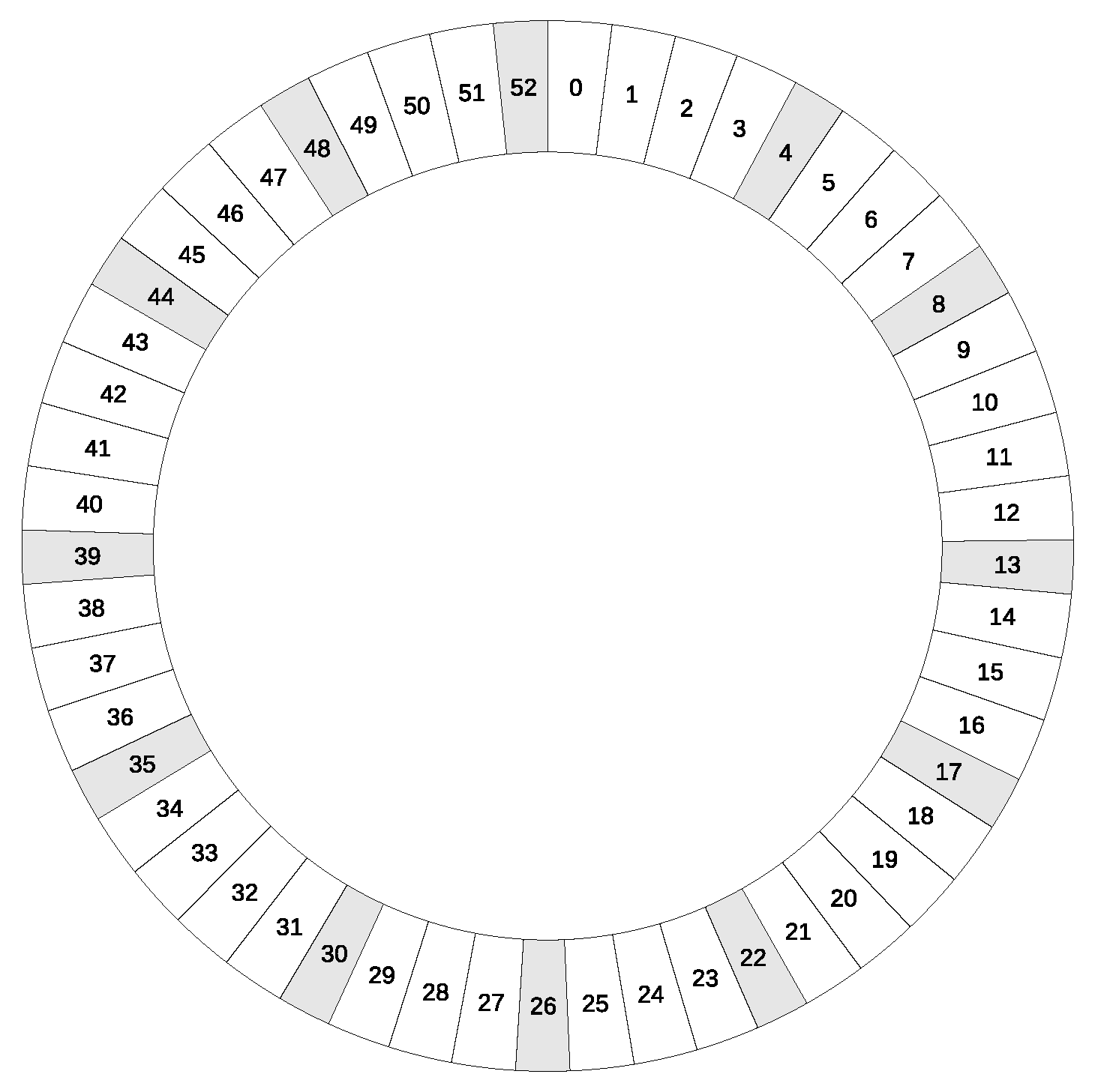
At the end of a lineage, the scale is regular by sections with at least two superdiatonic intervals (the more regular intervals, the more stages the lineage has) that are separated by a single subdiatonic interval. Figure 3 displays the last scale of the lineage 17 29 41 53 . The white intervals are the superdiatonic intervals (23.46¢), and the gray intervals are the subdiatonic intervals (19.84¢). The penultimate scale of the lineage is always optimal, i.e., corresponds to a convergent of the continued fraction expansion of the generator tone, although in this case, the last 53-tone scale is also optimal, which endows the scale with very interesting properties, since, in addition, it is of minimum bias and very close to an equal temperament scale.
It has been proven that the sum of the ruling indices up to the i-th stage is the number of tones of E n i g . For the last scale of a lineage, the number of subdiatones and superdiatones match the number of tones of both previous optimal scales.
Such an organization induces a partition into the scale defined by the two types of tones and intervals. How this diversity varies along a lineage has been analyzed through the Shannon diversity index based on entropy, either for an abundance of tones, h , or for occupancy of intervals, h.
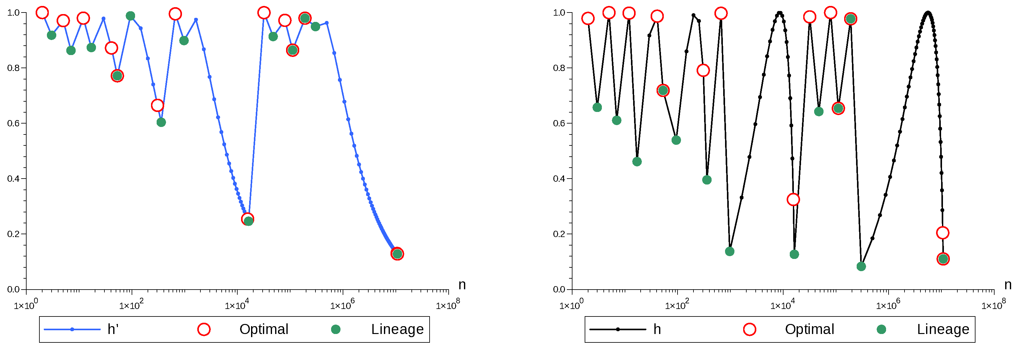
During a lineage, along the stages with the same ruling index, the abundance–diversity index h decreases, having a minimum at the end of a lineage. On the other hand, the occupancy–diversity index is low at the beginning of a non-short lineage after an optimal scale, meaning that there is a significant difference between the fraction of octave occupied by the diatonic and accidental intervals, in this way allowing the interval refinement. During the lineage, the occupancy–diversity index increases and decreases as the fractions of octave M u and m d change their relative proportions. Local minima of h take place at the beginning of non-short lineages.
Then, the regular refinement of one of the elementary intervals is determined by the beginning of a short lineage corresponding to a local minimum of h and by the end of a lineage corresponding to a local minimum of h .
Figure 4 displays the trend of the diversity indices in Pythagorean tuning. We point out the most interesting cases of non-short lineages for music scales with a reasonable number of tones, so to say, with 7 n 359 .
  • Where 7 12 17 . The lineage starts and ends at a local minimum of h and h. In each new stage, 5 (ruling index) new tones are regularly added. In the 17-tone scale, the diatonic elementary interval of the 7-tone scale has been split into two regular intervals, so that between the five subdiatones of the 17-tone scale we may find 2 or 3 equally spaced superdiatones out of 12.
  • Where 17 29 41 53 . The first stage is a local minimum of both h and h, the last one is a local minimum of h . In each next stage, 12 (ruling index) new microtones are regularly added. In the 53-tone scale, the diatonic elementary interval of the 17-tone scale has been split into three regular intervals, so that between the 12 subdiatones of the 53-tone scale, we may find 3 or 4 regularly distributed out of the 41 superdiatones.
  • Where 94 147 200 253 306 359 . The first stage is a local minimum of h, and the last stage is a local minimum of both, h and h. In each stage, 53 (ruling index) new microtones are regularly added. In the 359-tone scale, the diatonic elementary interval of the 94-tone scale has been split into five regular intervals, so that between the 53 subdiatones of the 94-tone scale, we may find 5 or 6 regularly distributed out of the 306 superdiatones.
In music, the lineage 7 12 17 has the following interpretation. For each tone of the heptatonic scale C, D, E, F, G, A, B, one has the possibility to choose between two accidentals on each side, i.e., C♯, D♯, F♯, G♯, A♯, plus D♭, E♭, G♭, A♭, B♭. Using these alternative accidentals is known as expressive intonation.
Some Middle-East music systems, such as the Ottoman, follow a similar approach by using added tones in the lineage 17 29 41 53 , where a selected row of tones are allowed to vary one Pythagorean comma up or down (23.46¢) to produce melodies with emotional intent or to tune to precise frequency ratios.
According to [33] (and references therein), Al-Kindi (ca. 800-873) was the first to make use of the Abjad (Arabic shorthand for “ABCD”) pitch notation to denote finger positions on the ud for his 12-note approach, which was purely Pythagorean. It was the precursor to Urmavi’s 17-tone scale (1216-1294), which added five additional backward fifth iterations. This is an example of the lineage 7 12 17 . On the other hand, several extensions of the 17-tone scale by adding sets of 12 fifths either backward or forward (such as the Arel-Ezgi-Uzdilek and Yekta variants) end in the 53-tone Pythagorean scale, which is very close to the 53 equal divisions of the octave. This scale is a common grid embracing the previous tunings, with 9 commas per whole tone, and 53 commas per octave. This comma is Holdrian, i.e., 22.64¢ wide, which is less than one cent error to the Pythagorean comma. This is an example of the lineage 17 29 41 53 .
For fretless instruments, the last scale of a non-short lineage makes it easy to accurately determine the position of the superdiatones by referring them to the subdiatones. In general, from a music theory perspective, this scale has more flexibility in relation to symmetry rotations of specific intervals.

Funding

This research received no external funding.

Data Availability Statement

Data are contained within the article.

Conflicts of Interest

The author declares no conflicts of interest.

References

  1. Cubarsi, R. Choosing the representative tones of an abstract Pythagorean scale with regard to just intonation. J. Math. Music. 2025, 19, 145–163. [Google Scholar] [CrossRef]
  2. Carey, N.; Clampitt, D. Aspects of Well-Formed Scales. Music Theory Spectr. 1989, 11, 187–206. [Google Scholar] [CrossRef]
  3. Carey, N.; Clampitt, D. Two Theorems Concerning Rational Approximations. J. Math. Music 2012, 6, 61–66. [Google Scholar] [CrossRef]
  4. Carey, N.; Clampitt, D. Addendum to ”Two Theorems Concerning Rational Approximations”. J. Math. Music 2017, 11, 61–63. [Google Scholar] [CrossRef]
  5. Wilson, E. Bosanquet–A Bridge–A Doorway to Dialog. Wilson Arch. 1974. Available online: https://www.anaphoria.com/xen2.pdf (accessed on 11 May 2025).
  6. Wilson, E. Letter to Chalmers Pertaining to Moments Of Symmetry/Tanabe Cycle. Wilson Arch. 1975. Available online: https://www.anaphoria.com/mos.pdf (accessed on 11 May 2025).
  7. Hellegouarch, Y. Gammes naturelles. Gaz. Mat. 1999, 81, 25–39. [Google Scholar]
  8. Hellegouarch, Y. Gammes naturelles II. Gaz. Mat. 1999, 82, 13–26. [Google Scholar]
  9. Cubarsi, R. An alternative approach to generalized Pythagorean scales. Generation and properties derived in the frequency domain. J. Math. Music 2020, 14, 266–291. [Google Scholar] [CrossRef]
  10. Cubarsi, R. On the divisions of the octave in generalized Pythagorean scales and their bidimensional representation. J. Math. Music 2024, 18, 1–19. [Google Scholar] [CrossRef]
  11. Savaş, E.; Mursaleen, M. Bézier Type Kantorovich q-Baskakov Operators via Wavelets and Some Approximation Properties. Bull. Iran. Math. Soc. 2023, 49, 68. [Google Scholar] [CrossRef]
  12. Cai, Q.B.; Aslan, R.; Özger, F.; Srivastava, H. Approximation by a new Stancu variant of generalized (λ,μ)-Bernstein operators. Alex. Eng. J. 2024, 107, 205–214. [Google Scholar] [CrossRef]
  13. Ansari, K.; Özger, F. Pointwise and weighted estimates for Bernstein-Kantorovich type operators including beta function. Indian J. Pure Appl. Math. 2024. [Google Scholar] [CrossRef]
  14. Berstel, J.; de Luca, A. Sturmian Words, Lyndon Words and Trees. Theor. Comput. Sci. 1997, 178, 171–203. [Google Scholar] [CrossRef]
  15. Regener, E. Pitch Notation and Equal Temperament: A Formal Study; University of California Press: Berkeley, CA, USA, 1973. [Google Scholar]
  16. Calkin, N.; Wilf, H. Recounting the Rationals. Amer. Math. Montly 2000, 107, 360–363. [Google Scholar] [CrossRef]
  17. Gibbons, J.; Lester, D.; Bird, R. Funtional Pearl: Enumerating the Rationals. J. Funct. Program. 2006, 16, 281–291. [Google Scholar] [CrossRef]
  18. Noll, T. Sturmian Sequences and Morphisms: A Music-Theoretical Application; Société Mathématique de France, Journée Annuelle: Paris, France, 2008; pp. 79–102. [Google Scholar]
  19. Clampitt, D.; Noll, T. Modes, the Height-Width Duality, and Handschin’s Tone Character. Music Theory Online 2011, 17, 1–43. [Google Scholar] [CrossRef]
  20. Noll, T. Triads as Modes Within Scales as Modes; Springer: Cham, Switzerland, 2015; Volume 9110, pp. 373–384. [Google Scholar]
  21. Snyder, J. Entropy as a Measure of Musical Style: The Influence of a Priori Assumptions. Music Theory Spectr. 1990, 12, 121–160. [Google Scholar] [CrossRef]
  22. Gündüz, G. Entropy, energy, and instability in music. Phys. A Stat. Mech. Its Appl. 2023, 609, 128365. [Google Scholar] [CrossRef]
  23. Cubarsi, R. Partition Entropy as a Measure of Regularity of Music Scales. Mathematics 2024, 12, 1658. [Google Scholar] [CrossRef]
  24. Mursaleen, M.; Serra-Capizzano, S. Statistical Convergence via q-Calculus and a Korovkin’s Type Approximation Theorem. Axioms 2022, 11, 70. [Google Scholar] [CrossRef]
  25. Alamer, A.; Nasiruzzaman, M. Approximation by Stancu variant of λ-Bernstein shifted knots operators associated by Bézier basis function. J. King Saud-Univ.-Sci. 2024, 36, 103333. [Google Scholar] [CrossRef]
  26. Clough, J.; Myerson, G. Variety and multiplicity in diatonic systems. J. Music Theory 1985, 29, 249–270. [Google Scholar] [CrossRef]
  27. Clough, J.; Myerson, G. Musical scales and the generalized circle of fifths. Am. Math. Mon. 1986, 93, 695–701. [Google Scholar] [CrossRef]
  28. Khinchin, A. Continued Fractions; University of Chicago: Chicago, IL, USA, 1964. [Google Scholar]
  29. Hančl, J.; Turek, O. One-sided Diophantine approximations. J. Phys. A Math. Theor. 2019, 52, 045205. [Google Scholar] [CrossRef]
  30. Loya, P. Amazing and Aesthetic Aspects of Analysis; Springer: New York, NY, USA, 2017. [Google Scholar]
  31. Lothaire, M. Algebraic Combinatorics on Words; Cambridge University Press: Cambridge, UK, 2002. [Google Scholar]
  32. Shannon, C. A Mathematical Theory of Communication. Bell Syst. Tech. J. 1948, 27, 379–423. [Google Scholar] [CrossRef]
  33. Yarman, O. A Comparative Evaluation of Pitch Notations in Turkish Makam Music. J. Interdiscip. Music. Stud. 2007, 1, 51–62. [Google Scholar] [CrossRef]
Figure 1. In each new cyclic scale, the greatest interval of the previous scale is split into one of equal size of the smallest interval and another one of the remaining size. The matching interval between the stages i 1 and i is the diatonic interval in the latter.
Axioms 14 00471 g001
Figure 2. Increasing diversity index h in the actual accidental’s range 0 < x < 1 2 .
Axioms 14 00471 g002
Figure 3. Scale resulting at the end of the lineage 17 29 41 53 . In gray are the 12 intervals associated with the subdiatones. In white are the 41 intervals associated with the superdiatones.
Axioms 14 00471 g003
Figure 4. Abundance and occupancy diversity indices, h and h. Red circles indicate optimal scales (n = 2, 5, 12, 41, 53, 306, …) and green disks a change of lineage (n = 3, 7, 17, 53, 94, 359, …).
Axioms 14 00471 g004
Table 1. Values referred to the i-th Pythagorean scale ( g = 3 ): n i (number of tones); m i , M i (indices of the minimum and maximum tones); δ i (0 or 1, depending on whether the closure is just below or above the fundamental). R i indicates the ruling index (marked with gray/white bands). The symbols ♀ and ♂ denote lineages of minimum or maximum tone, respectively. The beginning of a lineage is in bold. The symbol ↷ indicates an optimal scale (the digit δ i changes).
i n i m i M i δ i R i
22 1=10 ↷1
33Axioms 14 00471 i0012>111
452<3 1 ↷2
572<5Axioms 14 00471 i00202
612 7>50 ↷5
717Axioms 14 00471 i00112>515
82912<17 112
94112<29 1 ↷12
105312<41Axioms 14 00471 i0020 ↷12
1194Axioms 14 00471 i00153>41141
1214753<94 153
1320053<147 153
1425353<200 153
1530653<253 1 ↷53
1635953<306Axioms 14 00471 i002053
17665 359>3060 ↷306
18971Axioms 14 00471 i001665>3061306
191636665<971 1665
202301665<1636 1665
212966665<2301 1665
223631665<2966 1665
234296665<3631 1665
244961665<4296 1665
255626665<4961 1665
266291665<5626 1665
276956665<6291 1665
287621665<6956 1665
298286665<7621 1665
308951665<8286 1665
319616665<8951 1665
3210,281665<9616 1665
3310,946665<10,281 1665
3411,611665<10,946 1665
3512,276665<11,611 1665
3612,941665<12,276 1665
3713,606665<12,941 1665
3814,271665<13,606 1665
3914,936665<14,271 1665
4015,601665<14,936 1 ↷665
4116,266665<15,601Axioms 14 00471 i0020665
4231,867 16,266>15,6010 ↷15,601
4347,468Axioms 14 00471 i00131,867>15,601115,601
4479,33531,867<47,468 1 ↷31,867
45111,20231,867<79,335Axioms 14 00471 i0020 ↷31,867
46190,537Axioms 14 00471 i001111,202>79,3351 ↷79,335
47301,739111,202<190,537Axioms 14 00471 i0020111,202
48492,276301,739>190,5370190,537
49682,813492,276>190,5370190,537
50873,350682,813>190,5370190,537
511,063,887873,350>190,5370190,537
Table 2. The arrows indicate whether h decreases or increases depending on the values of δ . An optimal scale is marked in boldface and the beginning of a lineage with a gray background.
δ i 1 δ i δ i + 1 δ i + 2
(1)+(3b)001any
(4)+(2a)110any
(2b)+(3b)101any
(3a)+(2a)010any
Table 3. The arrows indicate whether h decreases or increases depending on the values of δ . An optimal scale is marked in boldface and the beginning of a lineage with a gray background.
δ i 1 δ i δ i + 1 δ i + 2
(1)+(3)+(4)0011
(4)+(2)+(1)1100
Disclaimer/Publisher’s Note: The statements, opinions and data contained in all publications are solely those of the individual author(s) and contributor(s) and not of MDPI and/or the editor(s). MDPI and/or the editor(s) disclaim responsibility for any injury to people or property resulting from any ideas, methods, instructions or products referred to in the content.

