Asymptotical Behavior of Impulsive Linearly Implicit Euler Method for the SIR Epidemic Model with Nonlinear Incidence Rates and Proportional Impulsive Vaccination

Abstract

This paper is concerned with the asymptotical behavior of the impulsive linearly implicit Euler method for the SIR epidemic model with nonlinear incidence rates and proportional impulsive vaccination. We point out the solution of the impulsive linearly implicit Euler method for the impulsive SIR system is positive for arbitrary step size when the initial values are positive. By applying discrete Floquet’s theorem and small-amplitude perturbation skills, we proved that the disease-free periodic solution of the impulsive system is locally stable. Additionally, in conjunction with the discrete impulsive comparison theorem, we show that the impulsive linearly implicit Euler method maintains the global asymptotical stability of the exact solution of the impulsive system. Two numerical examples are provided to illustrate the correctness of the results.

1. Introduction

Infectious diseases have always been a major threat to global public health, causing significant morbidity and mortality across populations. The study of epidemic dynamics has become crucial for understanding disease transmission patterns and developing effective control strategies. One of the most influential models in this field is the SIR (Susceptible–Infected–Recovered) model [1], which was first introduced by Kermack and McKendrick in 1927. This compartmental model divides the population into three categories: susceptible individuals who are at risk of infection, infected individuals who are capable of transmitting the disease, and recovered individuals who have immunity against the disease. The SIR model has since been widely applied to analyze various infectious diseases [2,3,4], including influenza, measles, and, more recently, COVID-19.

The concept of pulse vaccination, which involves administering vaccines to a large portion of the population at specific intervals, has gained significant attention as an effective strategy for controlling and eradicating infectious diseases [5,6,7]. This approach has proven particularly successful in reducing the prevalence of childhood diseases such as measles and polio. Although analytical methods have been successful in studying SIR models [8,9,10,11,12,13,14], obtaining accurate solutions for many pulse epidemic systems is often difficult or impossible. This challenge has led to the development of numerical methods for approximating the solution of the pulse SIR equation. Numerical methods not only provide insights into the behavior of epidemic models but also provide practical tools for public health decision-making. Therefore, it is important to study numerical methods for the impulsive SIR equations [15].

In recent years, the linearly implicit Euler method (LIEM) for SIR equations without impulsive perturbations has gained increasing attention as a very effective numerical method [16,17,18,19]. In [16], the authors proposed the LIEM numerical method thresholds for aged SIS models with finite maximum age, in which some numerical basic reproduction numbers were provided and the stability of the disease-free equilibrium was investigated. In [17], the authors studied a numerical reproduction number of the linearly implicit Euler–Riemann method for a single nonlinear age-structured population model with infinite age. In [18], a numerical threshold of a LIEM for a nonlinear infection-age SIR model was studied. In [15], the impulsive linear implicit Euler method (ILIEM) was first proposed to solve the SIR epidemic equation with a pulse vaccination strategy, and it was pointed out that the method has the advantages of keeping the exact solution positive and maintaining the global attractiveness of the disease-free periodic solution. To the best of our knowledge, ILIEM has not been applied to solve the SIR epidemic model with nonlinear incidence rates and proportional impulsive vaccination. The discrete Floquet’s theorem and small-amplitude perturbation skills are also first applied to prove that ILIEM maintains the local stability of the disease-free periodic exact solution without restrictions on the step sizes, and further, ILIEM maintains the global asymptotical stability of the exact solution.

The remaining part of this article is organized as follows. In Section 2, we present the results on the asymptotical stability of the disease-free periodic solution of the impulsive SIR system. In Section 3, the local stability of the disease-free periodic solution of ILIEM for the impulsive SIR system is studied. Moreover, the global asymptotical stability of ILIEM is studied. In Section 4, two numerical examples are given to illustrate the correctness of the conclusions. The Section 5 includes the conclusions and future works.

2. Asymptotical Stability of the Exact Solution

In epidemic dynamics, we usually divide the total population (N) into the following groups: susceptible (class S), infected (class I), and removed (class R). In this paper, we consider the impulsive SIR system in [20] as follows:

$$\left\{\begin{array}{l}\left.\begin{array}{c}\begin{array}{c}{\displaystyle \frac{dS}{dt}}=-K{I}^{2}S-bS+r_{1}R+bN,\hfill \\ {\displaystyle \frac{{\displaystyle dI}}{{\displaystyle dt}}}=K{I}^{2}S-(b+v)I,\hfill \\ {\displaystyle \frac{{\displaystyle dR}}{{\displaystyle dt}}}=vI-(b+r_1)R,\hfill \end{array}\end{array}\right\}t\ne kT,\hfill \\ \left.\begin{array}{c}\begin{array}{c}S\left(t^{+}\right)=(1-p)S\left(t\right),\hfill \\ I\left(t^{+}\right)=I\left(t\right),\hfill \\ R\left(t^{+}\right)=R\left(t\right)+pS\left(t\right),\hfill \end{array}\end{array}\right\}t=kT,\end{array}\right.$$

(1)

where N is the total population. It is assumed in this model that all newborn infants are susceptible. Here, b represents both birth rate and mortality rate, v is the rate of infected individuals entering the removed category, $r_1$ is the probability that an individual removed from the category loses immunity and enters the susceptible category. Here, $H(I,S)=KIS$ is a nonlinear incidence rate concerning S and I (see [20]), which implies that the number of infected individuals per unit of time is $H(I,S)I=K{I}^{2}S$. Pulse vaccination is applied as an impulse at the discrete time $kT$, where T is a positive real constant, $k\in {\mathbb{Z}}^{+}=\{1,2,\cdots \}$. The train of impulses generated by pulse vaccination in (1) creates jump discontinuities in both $S\left(t\right)$ and $R\left(t\right)$, where $S\left(t\right)$ suddenly decreases by the proportion p, and $R\left(t\right)$ suddenly increases by $pS\left(t\right)$, whenever $t=kT$. The solutions $S\left(t\right)$ and $R\left(t\right)$ of (1) are left-continuous at all points. $S\left(t\right)$ and $R\left(t\right)$ are right-continuous except for $t=kT$. At $t=kT$, the right limits of $S\left(t\right)$ and $R\left(t\right)$ exist, denoted as $S\left(t^{+}\right)$ and $R\left(t^{+}\right)$, respectively. The solution $I\left(t\right)$ of (1) is continuous at all points. At the initial time $t=0$, we only require that the right limit exists $S\left(0^{+}\right)=S_0$, $I\left(0^{+}\right)=I_0$ and $R\left(0^{+}\right)=R_0$. Throughout this paper, we always require that $S_0$, $I_0$, and $R_0$ are nonnegative initial values and satisfy $S_0+I_0+R_0=N_0$. Assume that $\alpha =b+r_1$ and $\beta =b+v$. From combining this with Equation (1), we can easily prove that the following equality

$$S\left(t\right)+I\left(t\right)+R\left(t\right)\equiv N_0$$

holds for all t. Consequently, we need only study the following subsystem:

$$\left\{\begin{array}{c}\left.\begin{array}{c}\begin{array}{c}{\displaystyle \frac{dS}{dt}}=-K{I}^{2}S-\alpha S+\alpha N_0-r_{1}I\hfill \\ {\displaystyle \frac{{\displaystyle dI}}{{\displaystyle dt}}}=K{I}^{2}S-\beta I\hfill \end{array}\end{array}\right\}t\ne kT,\hfill \\ \left.\begin{array}{c}\begin{array}{c}S\left(t^{+}\right)=(1-p)S\left(t\right)\hfill \\ I\left(t^{+}\right)=I\left(t\right)\hfill \end{array}\end{array}\right\}t=kT,\hfill \end{array}\right.$$

(2)

where initial values $S\left(0^{+}\right)=S_0$ and $I\left(0^{+}\right)=I_0$ satisfy $0\le S_0\le N_0$ and $0\le I_0\le N_0$. When $I\left(t\right)\equiv 0$, instead of the system (2), we only need to consider the following subsystem:

$$\left\{\begin{array}{cc}{S}^{\prime }\left(t\right)=-\alpha S\left(t\right)+\alpha N_0,\hfill & t\ne kT,k\in \mathbb{N}\hfill \\ S\left(k{T}^{+}\right)=(1-p)S\left(k{T}^{-}\right),\hfill & k\in \mathbb{N}.\hfill \end{array}\right.$$

(3)

Lemma 1 

([20]). System (3) has a globally stable positive periodic solution,

$$\tilde{S}\left(t\right)=N_0-{\displaystyle \frac{p{N}_0{\mathrm{e}}^{-\alpha (t-kT)}}{1-(1-p){\mathrm{e}}^{-\alpha T}}},t\in (kT,(k+1)T].$$

(4)

Theorem 1 

([20]). The disease-free periodic solution $(\tilde{S}\left(t\right),0)$ of (2) is locally stable without other additional conditions.

Theorem 2. 

If $R_0<1$, then the disease-free periodic solution $(\tilde{S}\left(t\right),0)$ of (2) is globally attractive, where $R_0={\beta }^{-1}K{N}_0^2\left({\displaystyle \frac{1-{\mathrm{e}}^{-\alpha T}}{1-(1-p){\mathrm{e}}^{-\alpha T}}}\right)$.

Proof. 

By the first equation of (2), we can obtain that

$$S^{\prime }\left(t\right)\le -\alpha S\left(t\right)+\alpha N_0.$$

(5)

Applying Lemma 1 and impulsive comparison theorem (Lemma 2.2 of [9]) or (Lemma 2.1 of [10]), for any small $\epsilon >0$, there exists a positive constant $t_1$ such that for $t>t_1$, the solution $S\left(t\right)$ of (2) satisfies

$$S\left(t\right)<\tilde{S}\left(t\right)+ϵ,\forall t>t_1.$$

(6)

Combining the second equation of (2), we can obtain that

$$I^{\prime }\left(t\right)\le K{I}^2\left(t\right)(\tilde{S}\left(t\right)+ϵ)-\beta I\left(t\right)\le \left(K{N}_0(\tilde{S}\left(t\right)+ϵ)-\beta \right)I\left(t\right).$$

(7)

Because $R_0<1$, we get, for a small enough $ϵ$,

$$K{N}_0(\tilde{S}\left(t\right)+ϵ)-\beta \le K{N}_0(\tilde{S}(kT-)+ϵ)-\beta =:-\sigma <0.$$

By the comparison theorem [21,22], we can obtain that there exists a constant C such that

$$I\left(t\right)\le {\mathrm{e}}^{-\sigma t}C,t>t_1,$$

which means $\underset{t\to +\infty }{lim}I\left(t\right)=0$. For any small ${\epsilon }_1>0$, there exists an integer $t_2$ such that $\left|I\left(t\right)\right|<{\epsilon }_1$, $t\ge t_2$. Hence, by the first equation of (2), we can obtain that

$$S^{\prime }\left(t\right)\ge -K{\epsilon }_1^{2}S\left(t\right)-\alpha S\left(t\right)+\alpha N_0-r_1{\epsilon }_1.$$

(8)

Next, we consider the following comparison system with pulse

$$\left\{\begin{array}{cc}{u}^{\prime }\left(t\right)=-(\alpha +K{\epsilon }_1^2)u\left(t\right)+\alpha N_0-r_1{\epsilon }_1,\hfill & t\ne kT,t>0,\hfill \\ u\left(t\right)=(1-p)u\left(t\right),\hfill & t=kT.\hfill \end{array}\right.$$

We can obtain the following periodic solution:

$$\tilde{u}\left(t\right)=\left(u^{*}-{\displaystyle \frac{\alpha N_0-r_1{\epsilon }_1}{\alpha +K{\epsilon }_1^2}}\right){\mathrm{e}}^{-(\alpha +K{\epsilon }_1^2)(t-kT)}+{\displaystyle \frac{\alpha N_0-r_1{\epsilon }_1}{\alpha +K{\epsilon }_1^2}},$$

(9)

where $u^{*}={\displaystyle \frac{(1-p)\left(1-{\mathrm{e}}^{-(\alpha +K{\epsilon }_1^2)T}\right)(\alpha N_0-r_1{\epsilon }_1)}{(\alpha +K{\epsilon }_1^2)\left(1-(1-p){\mathrm{e}}^{-(\alpha +K{\epsilon }_1^2)T}\right)}}$.

By impulsive comparison theorem (Lemma 2.2 of [9]) or (Lemma 2.1 of [10]), there exists a positive constant $t_3$ such that

$$S\left(t\right)\ge u\left(t\right)>\tilde{u}\left(t\right)-{\epsilon }_2,\forall t\ge t_3.$$

(10)

Since ${\epsilon }_1$ and ${\epsilon }_2$ are sufficiently small, $\tilde{S}\left(t\right)$ is globally attractive. Consequently, the infection-free periodic solution $(\tilde{S}\left(t\right),0)$ is also globally attractive. □

From Theorem 1 and Theorem 2, we can immediately draw the following conclusion.

Theorem 3. 

If $R_0<1$, then the disease-free periodic solution $(\tilde{S}\left(t\right),0)$ of (2) is globally asymptotically stable.

3. ILIEM for Impulsive SIR

ILIEM for the impulsive SIR system (1) takes the following form:

$$\left\{\begin{array}{l}\left.\begin{array}{c}\begin{array}{c}{S}_{k,l+1}=S_{k,l}+h\left(-K{I}_{k,l}^2{S}_{k,l+1}-b{S}_{k,l+1}+r_1{R}_{k,l+1}+b{N}_0\right)\hfill \\ I_{k,l+1}=I_{k,l}+h\left(K{I}_{k,l}^2{S}_{k,l+1}-(b+v)I_{k,l+1}\right)\hfill \\ R_{k,l+1}=R_{k,l}+h\left(v{I}_{k,l+1}-(b+r_1)R_{k,l+1}\right)\hfill \end{array}\end{array}\right\}k\in \mathbb{N},l\in \mathbb{A},\hfill \\ \left.\begin{array}{c}\begin{array}{c}{S}_{k+1,0}=(1-p)S_{k,m}\hfill \\ I_{k+1,0}=I_{k,m}\hfill \\ R_{k+1,0}=R_{k,m}+p{S}_{k,m}\hfill \end{array}\end{array}\right\}k\in \mathbb{N},\end{array}\right.$$

(11)

with initial values $S_{0,0}=S_0$, $I_{0,0}=I_0$, $R_{0,0}=R_0$, where the step size $h={\displaystyle \frac{T}{m}}$, m is a positive constant, and $\mathbb{N}=\{0,1,2,\cdots \}$. Here ${\mathbb{Z}}^{+}=\{1,2,\cdots \}$, $\mathbb{A}=\{0,1,2,\cdots ,m-1\}$ and $\mathbb{B}=\{0,1,2,\cdots ,m\}$. The discretization nodes $t_{k,l}$ satisfy $t_{k,l}=(km+l)ht=kT+lh$, $k\in \mathbb{N}$, $l\in \mathbb{B}$ and $t_{k,m}=t_{k+1,0}=kT$, $k\in {\mathbb{Z}}^{+}$. The numerical solutions $S_{k,l}$, $I_{k,l}$, and $R_{k,l}$ are approximations of $S\left(t_{k,l}\right)$, $I\left(t_{k,l}\right)$, and $R\left(t_{k,l}\right)$ ($k\in \mathbb{N}$, $l\in \mathbb{B}-\left\{0\right\}$), respectively. Similarly, $S_{k,0}$, $I_{k,0}$, and $R_{k,0}$ are approximations of $S\left(k{T}^{+}\right)$, $I\left(k{T}^{+}\right)$ and $R\left(k{T}^{+}\right)$ ($k\in \mathbb{N}$), respectively.

3.1. Advantages of ILIEM

In this subsection, we point out the advantages of ILIEM (11) for the impulsive SIR system (1). Compared to the impulsive explicit Euler method and the implicit Euler method, the numerical solution of ILIEM is positive for arbitrary step sizes when the initial values are positive, and ILIEM is less computationally expensive than the impulsive implicit Euler method. Additionally, as with the nature of the exact solution of (1), the total population is invariant, so it suffices to consider the impulsive system (2) with respect to S and I, which can also be seen as ILIEM for (2).

Theorem 4. 

For any solution $(S_{k,l},I_{k,l},R_{k,l})$ of (11), the total number $N_{k,l}=S_{k,l}+I_{k,l}+R_{k,l}$ satisfies $N_{k,l}\equiv N_0$, $\forall k\in \mathbb{N},\forall l\in \mathbb{B}$, if $S_0+I_0+R_0=N_0$.

Proof. 

By the first three equations of (11), we can obtain that

$$\begin{array}{cc}\hfill N_{k,l+1}& =N_{k,l}-hb(S_{k,l+1}+R_{k,l+1}+I_{k,l+1})+hb{N}_0\hfill \\ & =N_{k,l}-hb{N}_{k,l+1}+hb{N}_0,\forall k\in \mathbb{N},\forall l\in \mathbb{A},\hfill \end{array}$$

which implies that $N_{k,l+1}=N_0$, when $N_{k,l}=N_0$ ($\forall k\in \mathbb{N},\forall l\in \mathbb{A}$).

Obviously, according to the fourth to sixth equations of (11), we have

$$N_{k+1,0}=N_{k,m},\forall k\in \mathbb{N}.$$

Consequently, applying mathematical induction, we can show that $N_{k,l}=N_0,k\in \mathbb{N},l\in \mathbb{B}$. The proof has been completed. □

ILIEM (11) can be rewritten in the following form:

$$\left\{\begin{array}{l}\left.\begin{array}{c}\begin{array}{c}{S}_{k,l+1}={\displaystyle \frac{S_{k,l}+hb{N}_0+h{r}_1{R}_{k,l+1}}{1+hb+hK{I}_{k,l}^2}}\hfill \\ I_{k,l+1}={\displaystyle \frac{I_{k,l}+hK{I}_{k,l}^2{S}_{k,l+1}}{1+h(b+v)}}\hfill \\ R_{k,l+1}={\displaystyle \frac{R_{k,l}+hv{I}_{k,l+1}}{1+h(b+r_1)}}\hfill \end{array}\end{array}\right\}k\in \mathbb{N},l\in \mathbb{A},\hfill \\ \left.\begin{array}{c}\begin{array}{c}{S}_{k+1,0}=(1-p)S_{k,m}\hfill \\ I_{k+1,0}=I_{k,m}\hfill \\ R_{k+1,0}=R_{k,m}+p{S}_{k,m}\hfill \end{array}\end{array}\right\}k\in \mathbb{N},\hfill \end{array}\right.$$

(12)

with initial values $S_{0,0}=S_0$, $I_{0,0}=I_0$, $R_{0,0}=R_0$.

Theorem 5. 

When the initial values $S_0$, $I_0$, and $R_0$ are nonnegative, the solutions $S_{k,l}$, $I_{k,l}$, and $R_{k,l}$ of (12) are nonnegative for $\forall k\in \mathbb{N}$, $\forall h>0$. In particular, $S_{k,l}>0$, $I_{k,l}>0$ and $R_{k,l}>0$ when the initial values satisfy $S_0>0$, $I_0>0$, and $R_0>0$.

Proof. 

Write (12) in vector form:

$$\left[\begin{array}{c}{S}_{k,l+1}\\ I_{k,l+1}\\ R_{k,l+1}\end{array}\right]=\left[\begin{array}{c}{\displaystyle \frac{S_{k,l}+hb{N}_0}{1+hb+hK{I}_{k,l}^2}}\\ {\displaystyle \frac{I_{k,l}}{1+h(b+v)}}\\ {\displaystyle \frac{R_{k,l}}{1+h(b+r_1)}}\end{array}\right]+\left[\begin{array}{ccc}0& 0& A\\ B& 0& 0\\ 0& C& 0\end{array}\right]\left[\begin{array}{c}{S}_{k,l+1}\\ I_{k,l+1}\\ R_{k,l+1}\end{array}\right],$$

(13)

where

$$A={\displaystyle \frac{h{r}_1}{1+hb+hK{I}_{k,l}^2}},B={\displaystyle \frac{hK{I}_{k,l}^2}{1+h(b+v)}},C={\displaystyle \frac{hv}{1+h(b+r_1)}}.$$

By simplifying, we can obtain

$$P{X}_{k,l+1}=Q{X}_{k,l}+F,$$

(14)

where

$$\begin{array}{cc}{X}_{k,l}=\left[\begin{array}{c}{S}_{k,l}\\ I_{k,l}\\ R_{k,l}\end{array}\right],& F=\left[\begin{array}{c}{\displaystyle \frac{hb{N}_0}{1+hb+hK{I}_{k,l}}}\\ 0\\ 0\end{array}\right],\\ P=\left[\begin{array}{ccc}1& 0& -A\\ -B& 1& 0\\ 0& -C& 1\end{array}\right],& Q=\left[\begin{array}{ccc}{\displaystyle \frac{1}{1+hb+hK{I}_{k,l}^2}}& 0& 0\\ 0& {\displaystyle \frac{1}{1+h(b+v)}}& 0\\ 0& 0& {\displaystyle \frac{1}{1+hb+hK{I}_{k,l}^2}}\end{array}\right].\end{array}$$

Clearly, every element of matrix Q is positive, and every element of matrix F is nonnegative. By a simple calculation, we have

$$P^{-1}=\left[\begin{array}{ccc}{\displaystyle \frac{1}{1-ABC}}& {\displaystyle \frac{AC}{1-ABC}}& {\displaystyle \frac{A}{1-ABC}}\\ {\displaystyle \frac{B}{1-ABC}}& {\displaystyle \frac{1}{1-ABC}}& {\displaystyle \frac{AB}{1-ABC}}\\ {\displaystyle \frac{BC}{1-ABC}}& {\displaystyle \frac{C}{1-ABC}}& {\displaystyle \frac{1}{1-ABC}}\end{array}\right].$$

Because $ABC<1$, and $A>0$, $B>0$, $C>0$, we can obtain that each element of $P^{-1}$ is positive.

From (14), we have

$$X_{k,l+1}=P^{-1}Q{X}_{k,l}+P^{-1}F.$$

(15)

Consequently, $S_{k,l+1}>0$, $I_{k,l+1}>0$, $R_{k,l+1}>0$, when $S_0>0$, $I_0>0$, and $R_0>0$. □

From [23], we know that the expression of the impulsive explicit Euler method (IEEM) for the impulsive SIR system (1) is as follows:

$$\left\{\begin{array}{l}\left.\begin{array}{c}\begin{array}{c}{S}_{k,l+1}=S_{k,l}+h\left(-K{I}_{k,l}^2{S}_{k,l}-b{S}_{k,l}+r_1{R}_{k,l}+b{N}_0\right)\hfill \\ I_{k,l+1}=I_{k,l}+h\left(K{I}_{k,l}^2{S}_{k,l}-(b+v)I_{k,l}\right)\hfill \\ R_{k,l+1}=R_{k,l}+h\left(v{I}_{k,l}-(b+r_1)R_{k,l}\right)\hfill \end{array}\end{array}\right\}k\in \mathbb{N},l\in \mathbb{A},\hfill \\ \left.\begin{array}{c}\begin{array}{c}{S}_{k+1,0}=(1-p)S_{k,m}\hfill \\ I_{k+1,0}=I_{k,m}\hfill \\ R_{k+1,0}=R_{k,m}+p{S}_{k,m}\hfill \end{array}\end{array}\right\}k\in \mathbb{N}.\end{array}\right.$$

(16)

The IEEM (16) of the calculation is highly efficient, but $I_{k,l+1}=I_{k,l}+h(K{I}_{k,l}^2{S}_{k,l}-(b+v)I_{k,l})$ is possibly negative for some large $I_{k,l}>0$.

From [23], we know that the expression of the impulsive implicit Euler method (IIEM) for the impulsive SIR system (1) is as follows:

$$\left\{\begin{array}{l}\left.\begin{array}{c}\begin{array}{c}{S}_{k,l+1}=S_{k,l}+h\left(-K{I}_{k,l+1}^2{S}_{k,l+1}-b{S}_{k,l+1}+r_1{R}_{k,l+1}+b{N}_0\right)\hfill \\ I_{k,l+1}=I_{k,l}+h\left(K{I}_{k,l+1}^2{S}_{k,l+1}-(b+v)I_{k,l+1}\right)\hfill \\ R_{k,l+1}=R_{k,l}+h\left(v{I}_{k,l+1}-(b+r_1)R_{k,l+1}\right)\hfill \end{array}\end{array}\right\}k\in \mathbb{N},l\in \mathbb{A},\hfill \\ \left.\begin{array}{c}\begin{array}{c}{S}_{k+1,0}=(1-p)S_{k,m}\hfill \\ I_{k+1,0}=I_{k,m}\hfill \\ R_{k+1,0}=R_{k,m}+p{S}_{k,m}\hfill \end{array}\end{array}\right\}k\in \mathbb{N}.\end{array}\right.$$

(17)

So, $I_{k,l+1}$ is possibly negative. ILIM can be rewritten as (15), which can be solved similarly to IEEM (16) without having to solve nonlinear algebraic equations and with a lower computational cost than implicit methods (17).

3.2. Asymptotical Stability of ILIEM

In this subsection, we will apply discrete Floquet’s theorem and small-amplitude perturbation skills to study the local stability of the disease-free periodic solution of ILIEM for the impulsive system (2). Furthermore, we will study the global asymptotical stability of ILIEM when the disease-free periodic solution of the impulsive system (2) is globally stable.

From Theorem 4, we know that $N_0=S_{k,l}+I_{k,l}+R_{k,l}$, $\forall k\in \mathbb{N}$, $\forall l\in \mathbb{B}$. We only need to consider the following subsystem of (11), which can also be seen as ILIEM for (2),

$$\left\{\begin{array}{l}\left.\begin{array}{c}\begin{array}{c}{S}_{k,l+1}=S_{k,l}+h\left(-K{I}_{k,l}^2{S}_{k,l+1}-\alpha S_{k,l+1}+\alpha N_0-r_1{I}_{k,l+1}\right)\hfill \\ I_{k,l+1}=I_{k,l}+h\left(K{I}_{k,l}^2{S}_{k,l+1}-\beta I_{k,l+1}\right)\hfill \end{array}\end{array}\right\}k\in \mathbb{N},l\in \mathbb{A},\hfill \\ \left.\begin{array}{c}\begin{array}{c}{S}_{k+1,0}=(1-p)S_{k,m}\hfill \\ I_{k+1,0}=I_{k,m}\hfill \end{array}\end{array}\right\}k\in \mathbb{N},\end{array}\right.$$

(18)

with initial values $S_{0,0}=S_0\ge 0$, $I_{0,0}=I_0\ge 0$. By calculating this, we can rewrite (18) in the following explicit form:

$$\left\{\begin{array}{c}\left[\begin{array}{c}{S}_{k,l+1}\\ I_{k,l+1}\end{array}\right]=\left[\begin{array}{c}{\displaystyle \frac{\left(1+h\beta \right)\left(S_{k,l}+h\alpha N_0\right)}{\left(1+h\beta \right)\left(1+h\alpha +hK{I}_{k,l}^2\right)+h^{2}K{r}_1{I}_{k,l}^2}}-{\displaystyle \frac{h{r}_1{I}_{k,l}}{\left(1+h\beta \right)\left(1+h\alpha +hK{I}_{k,l}^2\right)+h^{2}K{r}_1{I}_{k,l}^2}}\\ {\displaystyle \frac{hK{I}_{k,l}^2\left(S_{k,l}+h\alpha N_0\right)}{\left(1+h\beta \right)\left(1+h\alpha +hK{I}_{k,l}^2\right)+h^{2}K{r}_1{I}_{k,l}^2}}+{\displaystyle \frac{I_{k,l}\left(1+h\alpha +hK{I}_{k,l}^2\right)}{\left(1+h\beta \right)\left(1+h\alpha +hK{I}_{k,l}^2\right)+h^{2}K{r}_1{I}_{k,l}^2}}\end{array}\right],k\in \mathbb{N},l\in \mathbb{A},\hfill \\ \left[\begin{array}{c}{x}_{k+1,0}\\ y_{k+1,0}\end{array}\right]=\left[\begin{array}{cc}1-p& 0\\ 0& 1\end{array}\right]\left[\begin{array}{c}{x}_{k,m}\\ y_{k,m}\end{array}\right],k\in \mathbb{N}.\hfill \end{array}\right.$$

(19)

Remark 1. 

From Theorem 4 and Theorem 5, we can immediately see that the solutions $S_{k,l}$, $I_{k,l}$ and $R_{k,l}$ of (12) satisfy $0\le S_{k,l}\le N_0$, $0\le I_{k,l}\le N_0$ and $0\le R_{k,l}\le N_0$, when the initial values satisfy $S_0\ge 0$, $I_0\ge 0$, $R_0\ge 0$ and $S_0+I_0+R_0=N_0$ (throughout the rest of this article, this condition is held by default).

Next, we will study the following subsystem (disease-free subsystem of (18)):

$$\left\{\begin{array}{cc}{S}_{k,l+1}=S_{k,l}-h\alpha S_{k,l+1}+h\alpha N_0,\hfill & k\in \mathbb{N},l\in \mathbb{A},\hfill \\ S_{k+1,0}=(1-p)S_{k,m},\hfill & k\in \mathbb{N}.\hfill \end{array}\right.$$

(20)

Applying (Lemma 1 of [15]) or (Lemma 5 of [24]), we immediately obtain the following result.

Lemma 2. 

System (20) has a globally asymptotically stable positive periodic solution

$${\tilde{S}}_{k,l}={\displaystyle \frac{S^{*}}{{(1+h\alpha )}^l}}+\left(1-{\displaystyle \frac{1}{{(1+h\alpha )}^l}}\right)N_0,\forall k\in \mathbb{N},l\in \mathbb{B},$$

(21)

where ${\tilde{S}}^{*}={\displaystyle \frac{(1-p)\left(1-{(1+h\alpha )}^{-m}\right)N_0}{1-(1-p){(1+h\alpha )}^{-m}}}$.

Obviously, the positive periodic solution (21) can also be written as follows:

$${\tilde{S}}_{k,l}=N_0-{\displaystyle \frac{p{N}_0{(1+h\alpha )}^{-l}}{1-(1-p){(1+h\alpha )}^{-m}}},\forall k\in \mathbb{N},l\in \mathbb{B}.$$

(22)

Lemma 3. 

The periodic solution ${\tilde{S}}_{k,l}$ in (21) of system (20) satisfies

$${\tilde{S}}_{k,l}\le {\tilde{S}}_{k,m},\forall k\in \mathbb{N},l\in \mathbb{B}.$$

Proof. 

We claim that $S^{*}\le N_0$ holds, because

$$N_0-{\tilde{S}}^{*}=N_0-{\displaystyle \frac{(1-p)\left(1-{(1+h\alpha )}^{-m}\right)N_0}{1-(1-p){(1+h\alpha )}^{-m}}}={\displaystyle \frac{p{N}_0}{1-(1-p){(1+h\alpha )}^{-m}}}\ge 0.$$

Consequently, the function

$$f\left(x\right)=x{\tilde{S}}^{*}+(1-x)N_0$$

is monotonically nondecreasing for $\forall x\in \mathbb{R}$, since $f^{\prime }\left(x\right)={\tilde{S}}^{*}-N_0\le 0$. Combined with the fact that ${(1+h\alpha )}^{-l}\ge {(1+h\alpha )}^{-m}$ holds for $l\le m$, we get

$$f\left({(1+h\alpha )}^{-l}\right)\le f\left({(1+h\alpha )}^{-m}\right);$$

that is, ${\tilde{S}}_{k,l}\le {\tilde{S}}_{k,m}$ holds for $\forall k\in \mathbb{N},l\in \mathbb{B}$. □

Theorem 6. 

The disease-free periodic solution $({\tilde{S}}_{k,l},0)$ of (18) is locally stable without other additional conditions.

Proof. 

Define

$$S_{k,l}=x_{k,l}+{\tilde{S}}_{k,l},I_{k,l}=y_{k,l},k\in \mathbb{N},l\in \mathbb{B}.$$

ILEIM of the form (19) can be expanded in a Taylor series: after neglecting higher order terms, the linearized equations read as

$$\left\{\begin{array}{c}\left[\begin{array}{c}{x}_{k,l+1}\\ y_{k,l+1}\end{array}\right]=\left[\begin{array}{cc}{\displaystyle \frac{1}{1+h\alpha }}& -{\displaystyle \frac{h{r}_1}{(1+h\alpha )(1+h\beta )}}\\ 0& {\displaystyle \frac{1}{1+h\beta }}\end{array}\right]\left[\begin{array}{c}{x}_{k,l}\\ y_{k,l}\end{array}\right],k\in \mathbb{N},l\in \mathbb{A},\hfill \\ \left[\begin{array}{c}{x}_{k+1,0}\\ y_{k+1,0}\end{array}\right]=\left[\begin{array}{cc}1-p& 0\\ 0& 1\end{array}\right]\left[\begin{array}{c}{x}_{k,m}\\ y_{k,m}\end{array}\right],k\in \mathbb{N}\hfill \end{array}\right.$$

To apply the discrete Floquet’s theorem ([25] or Lemma 3.1, Lemma 3.2 of [26]) to prove the result, we only need the following matrix,

$$M=\left[\begin{array}{cc}{\displaystyle \frac{(1-p)}{{(1+h\alpha )}^m}}& *\\ 0& {\displaystyle \frac{1}{{(1+h\beta )}^m}},\end{array}\right]$$

to have absolute values of its eigenvalues less than 1. If ${\lambda }_1$ and ${\lambda }_2$ are eigenvalues of matrix M, then ${\lambda }_1={\displaystyle \frac{(1-p)}{{(1+h\alpha )}^m}}$ and ${\lambda }_2={\displaystyle \frac{1}{{(1+h\beta )}^m}}$. Obviously, ${\lambda }_1<1$ and ${\lambda }_2<1$ for $\forall h={\displaystyle \frac{T}{m}}$ and $\forall m\in {\mathbb{Z}}^{+}$. □

Theorem 7. 

If $R_d<1$, then the disease-free periodic solution $({\tilde{S}}_{k,l},0)$ of (18) is globally attractive, where $R_d={\beta }^{-1}K{N}_0^2\left({\displaystyle \frac{1-{(1+h\alpha )}^{-m}}{1-(1-p){(1+h\alpha )}^{-m}}}\right)$.

Proof. 

By the first equation of (18), we can obtain that

$$S_{k,l+1}\le S_{k,l}-h\alpha S_{k,l+1}+h\alpha N_0.$$

(23)

Applying Lemma 2 and the impulsive comparison theorem, for any small $\epsilon >0$, there exists a positive constant $k_1$ such that for $k>k_1$, the solution $S_{k,l}$ of (18) satisfies

$$S_{k,l}<{\tilde{S}}_{k,l}+ϵ,\forall l\in \mathbb{B}.$$

(24)

Combining the second equation of (18), we can obtain that

$$I_{k,l+1}\le {\displaystyle \frac{I_{k,l}+hK{I}_{k,l}^2({\tilde{S}}_{k,l+1}+ϵ)}{1+h\beta }}\le \left({\displaystyle \frac{1+hK{N}_0({\tilde{S}}_{k,l+1}+ϵ)}{1+h\beta }}\right)I_{k,l}.$$

(25)

Applying Lemma 3, we get

$$I_{k+1,0}\le {\left({\displaystyle \frac{1+hK{N}_0({\tilde{S}}_{k,m}+ϵ)}{1+h\beta }}\right)}^m{I}_{k,0}.$$

(26)

Since $R_d<1$ means

$${\displaystyle \frac{K{N}_0({\tilde{S}}_{k,m}+ϵ)}{\beta }}<1,$$

the inequality (26) implies that $\underset{k\to +\infty }{lim}{I}_{k,l}=0$, $\forall l\in \mathbb{B}$. For any small ${\epsilon }_1>0$, there exists an integer $k_2$ such that $|I_{k,l}|<{\epsilon }_1$, $k\ge k_2$. Hence, by the first equation of (18), we can obtain that

$$S_{k,l+1}\ge {\displaystyle \frac{S_{k,l}+h\alpha N_0-h{r}_1{\epsilon }_1}{1+h\alpha +hK{\epsilon }_1^2}}.$$

(27)

Next, we consider the following comparison system with pulse

$$\left\{\begin{array}{cc}{u}_{k,l+1}={\displaystyle \frac{u_{k,l}+h\alpha N_0-h{r}_1{\epsilon }_1}{1+h\alpha +hK{\epsilon }_1^2}},\hfill & \forall k\in \mathbb{N},\forall l\in \mathbb{A},\hfill \\ u_{k+1,0}=(1-p)u_{k,m},\hfill & \forall k\in \mathbb{N}.\hfill \end{array}\right.$$

(28)

We can obtain the following periodic solution:

$${\tilde{u}}_{k,l}={(1+h\alpha +hK{\epsilon }_1^2)}^{-l}{u}^{*}+\left({\displaystyle \frac{1-{(1+h\alpha +hK{\epsilon }_1^2)}^{-l}}{h\alpha +hK{\epsilon }_1^2}}\right)(h\alpha N_0-h{r}_1{\epsilon }_1),$$

(29)

where $u^{*}={\displaystyle \frac{(1-p)\left(1-{(1+h\alpha +hK{\epsilon }_1^2)}^{-m}\right)(h\alpha -h{r}_1{\epsilon }_1)}{(h\alpha +hK{\epsilon }_1^2)\left(1-(1-p){(1+h\alpha +hK{\epsilon }_1^2)}^{-m}\right)}}$.

By the nonnegativity of $S_{k,l}$ and $u_{k,l}$, there exists an integer $k_3\in {\mathbb{Z}}^{+}$ such that

$$S_{k,l}\ge u_{k,l}>{\tilde{u}}_{k,l}-{\epsilon }_2,\forall k\ge k_3,\forall l\in \mathbb{B}.$$

(30)

Since ${\epsilon }_1$ and ${\epsilon }_2$ are sufficiently small, ${\tilde{S}}_{k,l}$ is globally attractive. Consequently, the infection-free periodic solution $({\tilde{S}}_{k,l},0)$ is also globally attractive. □

From Theorem 6 and Theorem 7, we can immediately draw the following conclusion:

Theorem 8. 

If $R_d<1$, then the disease-free periodic solution $({\tilde{S}}_{k,l},0)$ of (18) is globally asymptotically stable.

From Theorem 3, we know that the disease-free periodic solution of the system (2) is asymptotically stable under the condition $R_0<1$. We will further show below that the disease-free periodic solution $({\tilde{S}}_{k,l},0)$ of (18) is also asymptotically stable under the same conditions.

Theorem 9. 

If $R_0<1$, then the disease-free periodic solution $({\tilde{S}}_{k,l},0)$ of (18) is globally asymptotically stable.

Proof. 

To prove this result, we first consider the following function:

$$g\left(x\right)={\displaystyle \frac{1-x}{1-(1-p)x}},0\le x<1.$$

Obviously, $g^{\prime }\left(x\right)={\displaystyle \frac{-p}{{\left(1-(1-p)x\right)}^2}}<0$, which implies that $g\left(x\right)$ is monotonically decreasing.

In fact, we can easily obtain that

$${(1+h\alpha )}^m={(1+{\displaystyle \frac{T\alpha }{m}})}^{\left({\displaystyle \frac{m}{T\alpha }}\right)T\alpha }\le {\mathrm{e}}^{T\alpha },$$

which implies

$${(1+h\alpha )}^{-m}\ge {\mathrm{e}}^{-T\alpha }.$$

Hence,

$$g\left({(1+h\alpha )}^{-m}\right)\le g\left({\mathrm{e}}^{-T\alpha }\right),$$

which implies $R_d\le R_0<1$. Applying Theorem 8, we know the conclusion stands. □

Theorem 10. 

At any fixed time t ($t\in (kT,(k+1\left)T\right]$, $k\in N$), the limit of the discrete disease-free periodic solution $({\tilde{S}}_{k,l},0)$ of (18) is $(\tilde{S}\left(t\right),0)$ of the impulsive system (2) as h tends to 0. In this sense,

$$\underset{h\to 0,mh=\tau ,t=(km+l)h}{lim}({\tilde{S}}_{k,l},0)=(\tilde{S}\left(t\right),0).$$

Proof. 

Obviously, we have

$$\underset{h\to 0,mh=T,t=(km+l)h}{lim}{\left(1+h\alpha \right)}^m=\underset{h\to 0,mh=T,t=(km+l)h}{lim}{\left(1+{\displaystyle \frac{\alpha T}{m}}\right)}^{\left({\displaystyle \frac{m}{\alpha T}}\right)\alpha T}=e^{\alpha T},$$

and

$$\underset{h\to 0,mh=T,t=(km+l)h}{lim}{\left(1+h\alpha \right)}^l=\underset{h\to 0,mh=T,t=(km+l)h}{lim}{\left(1+{\displaystyle \frac{\alpha T}{m}}\right)}^{\left({\displaystyle \frac{m}{\alpha T}}\right)\left({\displaystyle \frac{l\alpha T}{m}}\right)}=e^{\alpha (t-kT)}.$$

From the two equalities above and expressions (4) and (22), it follows that

$$\underset{h\to 0,mh=T,t=(km+l)h}{lim}{\tilde{S}}_{k,l}=\tilde{S}\left(t\right).$$

(31)

End of proof. □

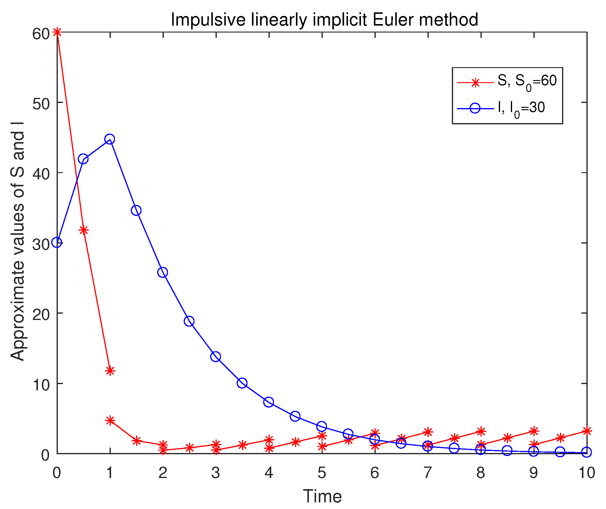
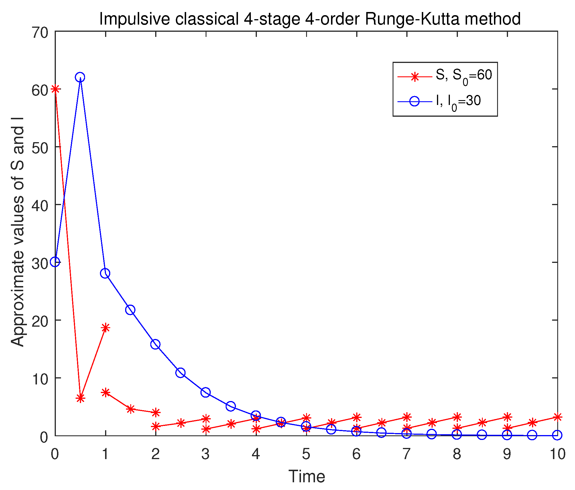
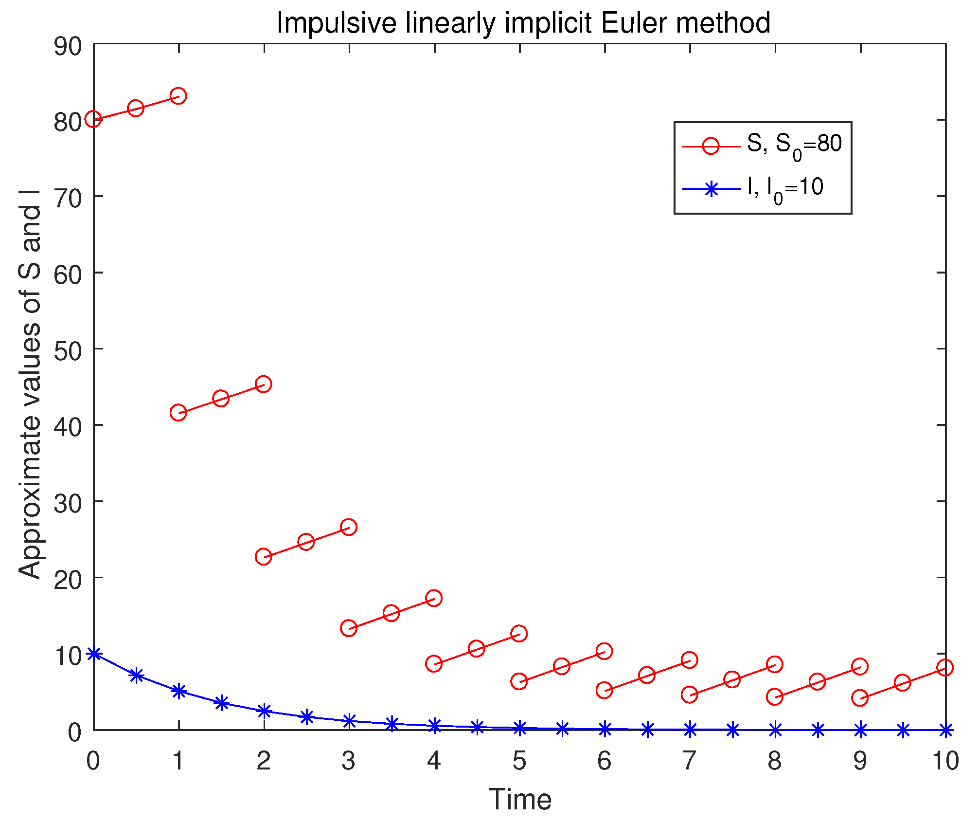
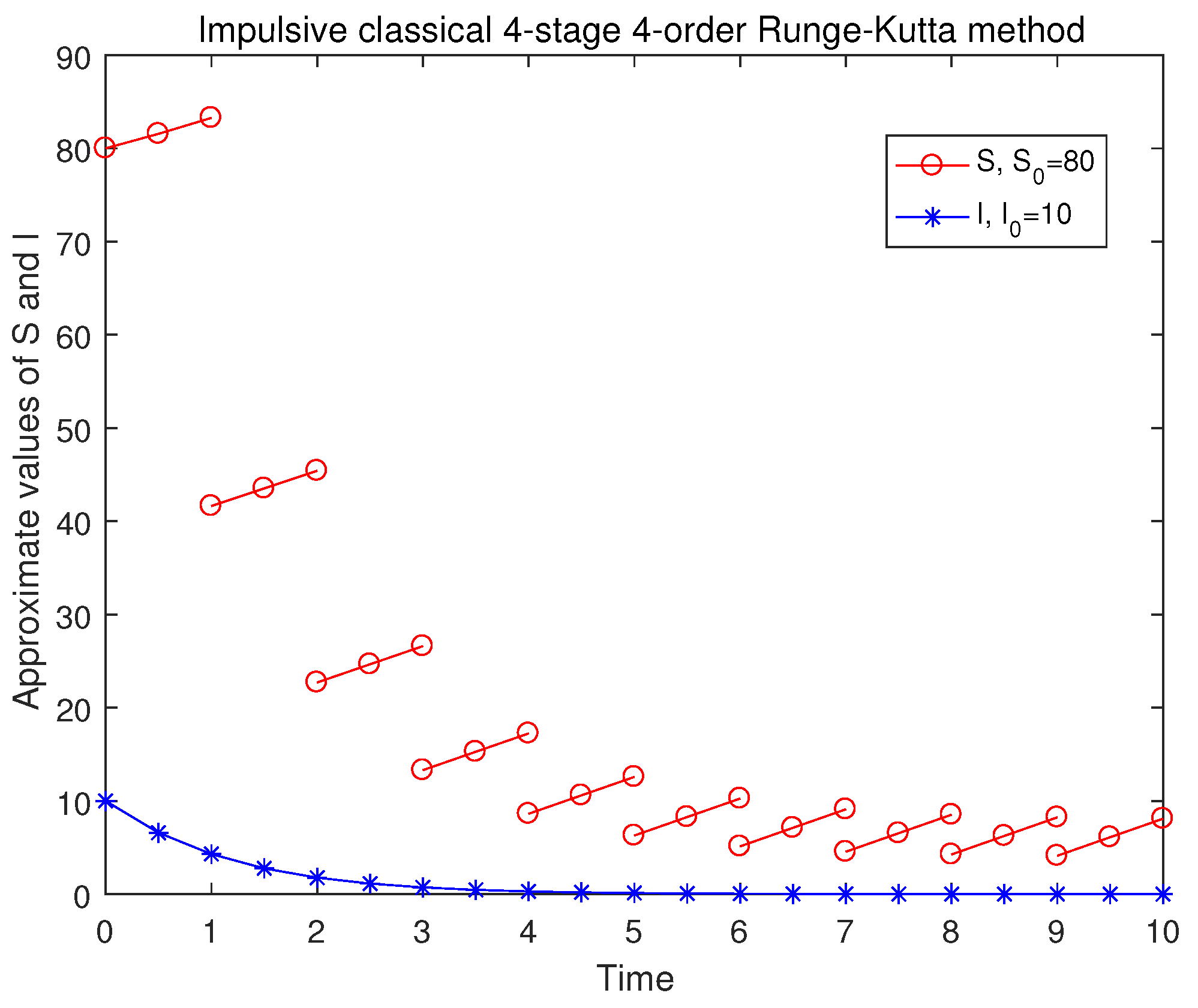
4. Numerical Experiments

In the following, two examples are provided to illustrate the correctness of the theory obtained above.

Example 1. 

The coefficients of the impulsive SIR system (2) were chosen to be $N_0=100$, $p=0.6$, $K=0.002$, $\alpha =0.02$, $T=1$, $\beta =0.5$, $r_1=0.01$. By calculation, it can be obtained that

$$R_0={\beta }^{-1}K{N}_0^2\left({\displaystyle \frac{1-{\mathrm{e}}^{-\alpha T}}{1-(1-p){\mathrm{e}}^{-\alpha T}}}\right)\approx 0.814306<1.$$

By Theorem 3, we can obtain that the disease-free periodic solution $(\tilde{S}\left(t\right),0)$ of (2) is globally asymptotically stable, where

$$\tilde{S}\left(t\right)=100-{\displaystyle \frac{60{\mathrm{e}}^{-0.02(t-k)}}{1-0.4{\mathrm{e}}^{-0.02}}},t\in (k,k+1],\forall k\in \mathbb{N}.$$

(32)

Additionally, using Theorem 9, the disease-free periodic solution $({\tilde{S}}_{k,l},0)$ of (18) is also globally asymptotically stable, where

$${\tilde{S}}_{k,l}=100-{\displaystyle \frac{60{(1+0.02h)}^{-l}}{1-0.4{(1+0.02h)}^{-m}}},\forall k\in \mathbb{N},l\in \mathbb{B}.$$

(33)

From (32) and (33), we can see that for arbitrary fixed t,

$$\underset{h\to 0,mh=1,t=(km+l)h}{lim}{\tilde{S}}_{k,l}=\tilde{S}\left(t\right),$$

which confirms the correctness of Theorem 10.

It is difficult to see the difference between Figure 1 and Figure 2, and between Figure 3 and Figure 4, from which it can be roughly seen that the error between the exact solution and the numerical solution of ILIEM is small. This can also be seen in

Table 1. The global errors between numerical solutions and exact solutions of (2) at $t=3$ when $N_0=100$, $p=0.8$, $K=0.002$, $\alpha =0.02$, $r_1=0.01$, $T=1$, $\beta =0.8$, with initial values $S_0=60$, $I_0=30$.

m	ILIEM	IEEM	IHM	ICRKM
1000	0.013948	0.032256	3.796751 × 10−10	2.135055 × 10−4
2000	0.006978	0.016134	4.013805 × 10−11	1.238906 × 10−5
4000	0.003490	0.008045	2.039033 × 10−12	7.846188 × 10−7
8000	0.001745	0.004014	2.548791 × 10−13	4.961802 × 10−8
Ratio	0.500168	0.499246	0.093839	0.061429

and

Table 2. The global errors between the numerical and exact solutions of (2) at $t=3$, when $N_0=1000$, $p=0.5$, $K=0.0001$, $\alpha =0.004$, $r_1=0.002$, $T=1$, $\beta =0.9$, with initial values $S_0=800$, $I_0=100$.

m	ILIEM	IEEM	IHM	ICRKM
1000	0.168657	3.408964 × 10−4	2.235798 × 10−6	1.983242 × 10−8
2000	0.084532	1.856005 × 10−4	2.815079 × 10−7	1.110038 × 10−9
4000	0.042318	9.799084 × 10−5	3.520072 × 10−8	6.243786 × 10−11
8000	0.021172	5.044188 × 10−5	4.285831 × 10−9	3.902366 × 10−12
Ratio	0.500709	0.528780	0.124210	0.058089

. Therefore, ILIEM is a very suitable numerical method.

Example 2. 

The coefficients of the impulsive SIR system (2) were chosen to be $N_0=1000$, $p=0.5$, $K=0.0001$, $\alpha =0.004$, $r_1=0.002$, $T=1$, $\beta =0.9$. By calculation, it can be obtained that

$$R_0={\beta }^{-1}K{N}_0^2\left({\displaystyle \frac{1-{\mathrm{e}}^{-\alpha T}}{1-(1-p){\mathrm{e}}^{-\alpha T}}}\right)\approx 0.883586<1.$$

By Theorem 3, we can obtain that the disease-free periodic solution $(\tilde{S}\left(t\right),0)$ of (2) is globally asymptotically stable, where

$$\tilde{S}\left(t\right)=1000-{\displaystyle \frac{500{\mathrm{e}}^{-0.004(t-k)}}{1-0.5{\mathrm{e}}^{-0.004}}},t\in (k,k+1],\forall k\in \mathbb{N}.$$

(34)

Furthermore, using Theorem 9, the disease-free periodic solution $({\tilde{S}}_{k,l},0)$ of (18) is also globally asymptotically stable, where

$${\tilde{S}}_{k,l}=1000-{\displaystyle \frac{500{(1+0.004h)}^{-l}}{1-0.5{(1+0.004h)}^{-m}}},\forall k\in \mathbb{N},l\in \mathbb{B}.$$

(35)

From (34) and (35), we can see that for arbitrary fixed t,

$$\underset{h\to 0,mh=4,t=(km+l)h}{lim}{\tilde{S}}_{k,l}=\tilde{S}\left(t\right),$$

which confirms the correctness of Theorem 10.

Table 1 and Table 2 present the global absolute errors (in Euclidean norm) between the exact solutions and the numerical solutions of the impulsive SIR system (2). We can see that the errors of ILIEM (18) and IEEM for (2) become half of the original error when the step sizes become half of the original, which roughly illustrates that both ILIEM (2) and IEEM for (2) are convergent of order 1.

Similarly, it can be seen that the errors of the impulsive 3-order Heun method (IHM) for (2) become approximately ${\displaystyle \frac{1}{8}}$ of the original errors when the step sizes become half of the original, which roughly illustrates that IHM for (2) is convergent of order 3. It can also be seen that the errors of the impulsive classical 4-stage 4-order Runge–Kutta method (ICRKM) for (2) become approximately ${\displaystyle \frac{1}{16}}$ of the original error when the step sizes become half of the original, which roughly illustrates that ICRKM for (2) is convergent of order 4.

5. Conclusions and Future Works

The ILIEM (11) for the impulsive SIR system (1) has the advantage of maintaining the nonnegativity of the exact solution, as well as the invariance of the population sum. By applying discrete Floquet’s theorem and small-amplitude perturbation skills, we proved that the disease-free periodic solution of the impulsive system (2) is locally stable. Additionally, in conjunction with the discrete impulsive comparison theorem, it is shown that the ILIEM (18) maintains the global asymptotic stability of the exact solution of (2).

In [20], the authors pointed out that the complex dynamics of system (2) depend on vaccination proportion p when the epidemic cannot be eliminated. The system may undergo a quasi-periodic solution, a multi-periodic solution, a strange attractor, or chaos. Whether the numerical solution of ILIEM (18) for the system (2) has the prior phenomena of a quasi-periodic solution, multi-periodic solution, singular attractor, or chaos requires further investigation. Whether the methods of [27,28] can be used to study the numerical solution of infectious disease models with delayed and stochastic effects will also be an important question for us to investigate in the future.

References

1. Kermack, W.O.; McKendrick, A.G. Contributions to the mathematical theory of epidemics. Proc. Roy. Soc. 1927, 115, 700–721. [Google Scholar]
2. Anderson, R.M.; May, R.M. Infectious Diseases of Humans: Dynamics and Control; Oxford University Press: Oxford, UK, 1991. [Google Scholar]
3. Ma, Z.E.; Zhou, Y.C.; Wu, J.H. Modeling and Dynamics of Infectious Diseases; Higher Education Press: Beijing, China, 2009. [Google Scholar]
4. Brauer, F.; Chavez, C.C.; Feng, Z.L. Mathematical Models in Epidemiology; Springer: New York, NY, USA, 2019. [Google Scholar]
5. Agur, Z.; Cojocaru, L.; Mazor, G.; Anderson, R.M.; Danon, Y.L. Pulse mass measles vaccination across age cohorts. Proc. Natl. Acad. Sci. USA 1993, 90, 11698–11702. [Google Scholar] [CrossRef] [PubMed]
6. Shulgin, B.; Stone, L.; Agur, Z. Pulse vaccination strategy in the SIR epidemic model. Bull. Math. Biol. 1998, 60, 1123–1148. [Google Scholar] [CrossRef] [PubMed]
7. Stone, L.; Shulgin, B.; Agur, Z. Theoretical examination of the pulse vaccination policy in the SIR epidemic model. Math. Comput. Model. 2000, 31, 207–215. [Google Scholar] [CrossRef]
8. Tang, S.Y.; Xiao, Y.N.; Clancy, D. New modelling approach concerning integrated disease control and cost-effectivity. Nonlinear Anal. 2005, 63, 439–471. [Google Scholar] [CrossRef]
9. Gao, S.J.; Chen, L.S.; Nieto, J.J.; Torres, A. Analysis of a delayed epidemic model with pulse vaccination and saturation incidence. Vaccine 2006, 24, 6037–6045. [Google Scholar] [CrossRef]
10. Gao, S.J.; Teng, Z.D.; Xie, D.H. Analysis of a delayed SIR epidemic model with pulse vaccination. Chaos Solitons Fractals 2009, 40, 1004–1011. [Google Scholar] [CrossRef]
11. Zhang, X.B.; Huo, H.F.; Sun, X.K.; Fu, Q. The differential susceptibility SIR epidemic model with time delay and pulse vaccination. J. Appl. Math. Comput. 2010, 34, 287–298. [Google Scholar] [CrossRef]
12. Li, M.Y.; Smith, H.L.; Wang, L. Global dynamics of an SEIR epidemic model with vertical transmission. SIAM J. Appl. Math. 2001, 62, 58–69. [Google Scholar] [CrossRef]
13. Chontita, R.; Inthira, C. A mathematical model for predicting and controlling COVID-19 transmission with impulsive vaccination. AIMS Math. 2024, 9, 6281–6304. [Google Scholar]
14. João, P.S.M.C.; Rodrigues, A.A. Pulse vaccination in a SIR model: Global dynamics, bifurcations and seasonality. Commun. Nonlinear Sci. Numer. Simul. 2024, 139, 108272. [Google Scholar]
15. Zhang, G.L.; Zhu, Z.Y.; Chen, L.K.; Liu, S.S. Impulsive linearly implicit Euler method for the SIR epidemic model with pulse vaccination strategy. Axioms 2024, 13, 854. [Google Scholar] [CrossRef]
16. Iannelli, M.; Milner, F.A.; Pugliese, A. Analytical and numerical results for the age structured SIS epidemic model with mixed inter-intracohort transmission. SIAM J. Math. Anal. 1992, 23, 662–688. [Google Scholar] [CrossRef]
17. Yang, Z.W.; Zuo, T.Q.; Chen, Z.J. Numerical analysis of linearly implicit Euler–Riemann method for nonlinear Gurtin-MacCamy model. Appl. Numer. Math. 2021, 163, 147–166. [Google Scholar] [CrossRef]
18. Yang, H.Z.; Yang, Z.W.; Liu, S.Q. Numerical threshold of linearly implicit Euler method for nonlinear infection-age SIR models. Discret. Contin. Dyn. Syst. Ser. B 2023, 28, 70–92. [Google Scholar] [CrossRef]
19. Cao, S.X.; Chen, Z.J.; Yang, Z.W. Numerical representations of global epidemic threshold for nonlinear infection-age SIR models. Math. Comput. Simul. 2023, 204, 115–132. [Google Scholar] [CrossRef]
20. Zeng, G.Z.; Chen, L.S. Complexity and asymptotical behavior of a SIRS epidemic model with proportional impulsive vaccination. Adv. Complex Syst. 2005, 8, 419–431. [Google Scholar] [CrossRef]
21. Ma, Z.E.; Zhou, Y.C.; Li, C.Z. Qualitative and Stability Methods for Ordinary Differential Equations; Science Press: Beijing, China, 2015. (In Chinese) [Google Scholar]
22. Hairer, E.; Nørsett, S.P.; Wanner, G. Solving Ordinary Differential Equations I; Nonstiff Problems; Springer: New York, NY, USA, 1993. [Google Scholar]
23. Zhang, G.L. Convergence, consistency and zero stability of impulsive one-step numerical methods. Appl. Math. Comput. 2022, 423, 127017. [Google Scholar] [CrossRef]
24. Sekiguchia, M.; Ishiwata, E. Dynamics of a discretized SIR epidemic model with pulse vaccination and time delay. J. Comput. Appl. Math. 2011, 236, 997–1008. [Google Scholar] [CrossRef]
25. Elaydi, S. An Introduction to Difference Equations; Springer: New York, NY, USA, 2005. [Google Scholar]
26. Liang, H.; Liu, M.Z.; Song, M.H. Extinction and permanence of the numerical solution of a two-prey one predator system with impulsive effect. Int. J. Comput. Math. 2011, 88, 1305–1325. [Google Scholar] [CrossRef]
27. Ding, X.H.; Wu, K.N.; Liu, M.Z. The Euler scheme and its convergence for impulsive delay differential equations. Appl. Math. Comput. 2010, 216, 1566–1570. [Google Scholar] [CrossRef]
28. Wu, K.N.; Ding, X.H. Convergence and stability of Euler method for impulsive stochastic delay differential equations. Appl. Math. Comput. 2014, 229, 151–158. [Google Scholar] [CrossRef]
Figure 1. ILIEM for (2) as N 0 = 100 , p = 0.6 , K = 0.002 , α = 0.02 , T = 1 , β = 0.5 , r 1 = 0.01 and h = 1 2 .
Axioms 14 00470 g001
Figure 2. Impulsive classical 4-stage 4-order Runge–Kutta method for (2) as N 0 = 100 , p = 0.6 , K = 0.002 , α = 0.02 , T = 1 , β = 0.5 , r 1 = 0.01 and h = 1 2 .
Axioms 14 00470 g002
Figure 3. ILIEM for (2) as N 0 = 100 , p = 0.5, K = 0.0001 , α = 0.004 , r 1 = 0.002 , T = 1 , β = 0.9 and h = 1 2 .
Axioms 14 00470 g003
Figure 4. Impulsive classical 4-stage 4-order Runge–Kutta method for (2) as N 0 = 100 , p = 0.5, K = 0.0001 , α = 0.004 , r 1 = 0.002 , T = 1 , β = 0.9 and h = 1 2 .
Axioms 14 00470 g004