Szász–Beta Operators Linking Frobenius–Euler–Simsek-Type Polynomials

Abstract

This manuscript associates with a study of Frobenius–Euler–Simsek-type Polynomials. In this research work, we construct a new sequence of Szász–Beta type operators via Frobenius–Euler–Simsek-type Polynomials to discuss approximation properties for the Lebesgue integrable functions, i.e., $L^p[0,\infty )$, $1\le p<\infty$. Furthermore, estimates in view of test functions and central moments are studied. Next, rate of convergence is discussed with the aid of the Korovkin theorem and the Voronovskaja type theorem. Moreover, direct approximation results in terms of modulus of continuity of first- and second-order, Peetre’s K-functional, Lipschitz type space, and the $r^{th}$-order Lipschitz type maximal functions are investigated. In the subsequent section, we present weighted approximation results, and statistical approximation theorems are discussed. To demonstrate the effectiveness and applicability of the proposed operators, we present several illustrative examples and visualize the results graphically.

1. Introduction

The systematic development of operator theory began in the late 19th century. An important aspect of approximation in operator theory is to find simple, computationally tractable approximations that capture the essential properties of more complex functions. These approximations can then be used for analysis, simulation, or computation in various applications, such as quantum mechanics, signal processing, and control theory. It provides powerful tools for solving problems and analyzing systems involving operators. In the last decade, there has been continued research and development in approximation theory in operator theory, with a focus on more advanced techniques having applications in data science and machine learning. In approximation theory, Weierstrass (1885) [1] formulated an elegant result known as the Weierstrass approximation theorem. Proving this theorem in a more straightforward and comprehensible manner has been the focus of several prominent mathematicians.

Bernstein (1912) [2] developed a sequence of polynomials called Bernstein polynomials to give a concise demonstration of Weierstrass approximation theorem using binomial distribution as:

$$\begin{array}{c}\hfill B_{\mathfrak{s}}(\Phi ;v)=\sum _{\vartheta =0}^{\mathfrak{s}}\Phi \left({\displaystyle \frac{\vartheta }{\mathfrak{s}}}\right)\left(\begin{array}{c}\mathfrak{s}\hfill \\ \vartheta \hfill \end{array}\right)v^{\vartheta }{(1-v)}^{\mathfrak{s}-\vartheta },v\in [0,1],\end{array}$$

(1)

where $\Phi$ is a continuous and bounded function on $[0,1]$. The operators in (1) restrict the approximation for continuous functions on bounded interval $[0,1]$. In order to discuss approximation properties on unbounded interval $[0,\infty )$, Szász [3] provided the modification to the operators in (1), which has played a significant role in the evolution of operator theory, as follows:

$$\begin{array}{c}\hfill S_{\mathfrak{s}}(\Phi ;v)=e^{-\mathfrak{s}v}\sum _{\vartheta =0}^{\infty }{\displaystyle \frac{{\left(\mathfrak{s}v\right)}^{\vartheta }}{\vartheta !}}\Phi \left({\displaystyle \frac{\vartheta }{\mathfrak{s}}}\right),\mathfrak{s}\in \mathbb{N},\end{array}$$

(2)

where real valued function $\Phi \in C[0,\infty )$. As given in (2), the linear positive operators are solely limited to continuous functional space. Many integral variants of these sequences of operators are obtained in order to approximate the longer class of functions, i.e., Lebesgue measurable functional space, Szász–Durremeyer and Szász–Kantorovich type operators, etc. ([4,5]). Many researchers, e.g., Acu et al. ([6,7]), Mohiuddine et al. ([8,9]), Mursaleen et al. ([10,11]), Khan et al. [12], Nasiruzzaman [13], and Rao et al. ([14,15,16,17]), have provided a number of generalizations for these kinds of sequences to investigate flexibility in approximation properties across several functional spaces.

In 2021, Simsek defined Frobenius–Euler–Simsek-type polynomials and numbers. He investigated the relations and identities between these special polynomials and numbers, such as Fubini polynomials and numbers and Bernoulli polynomials and numbers [18]. The Frobenius–Euler–Simsek-type polynomial $t_{\vartheta }(v;p)$ has a generating function given as:

$$F_t(v;w,p)={\displaystyle \frac{w^p}{{\displaystyle \prod _{l=0}^{p-1}}(e^w-l)}}{e}^{wv}=\sum _{\vartheta =0}^{\infty }{t}_{\vartheta }(v;p){\displaystyle \frac{w^{\vartheta }}{\vartheta !}}.$$

Taking p = 2, we have

$$F_t(v;w,2)={\displaystyle \frac{w^2}{e^w(e^w-1)}}{e}^{wv}=\sum _{\vartheta =0}^{\infty }{t}_{\vartheta }(v;2){\displaystyle \frac{w^{\vartheta }}{\vartheta !}}.$$

(3)

For more information on Euler-type polynomials and their applications, see also [19,20].

2. Construction of Operators

By the motivation from the definition of Frobenius–Euler–Simsek-type polynomials in Equation (3) with $w=1$, we present a sequence of positive and linear Szász–Beta operators to provide approximations in larger functional space, i.e., Lebesgue measurable functional space $L^p[0,\infty )$, for $v\in {\mathbb{R}}_0^{+}$ and $\Phi \in L^p[0,\infty )$ as:

$$\begin{array}{ccc}\hfill {\mathfrak{F}}_{\mathfrak{s}}(\Phi ;v)& =& (e^2-e)e^{-\mathfrak{s}v}\sum _{\vartheta =0}^{\infty }{\displaystyle \frac{t_{\vartheta }(\mathfrak{s}v;2)}{\vartheta !}}\underset{0}{\overset{\infty }{\int }}{Q}_{\mathfrak{s}}^{\vartheta }\left(u\right)\Phi \left(u\right)du,\hfill \end{array}$$

(4)

where $Q_{\mathfrak{s}}^{\vartheta }\left(u\right)={\displaystyle \frac{1}{\beta (\vartheta +1,\mathfrak{s})}}\left[{\displaystyle \frac{u^{\vartheta }}{{(1+u)}^{\vartheta +1+\mathfrak{s}}}}\right]$, Beta function, $\beta (\vartheta +1,\mathfrak{s})=\underset{0}{\overset{\infty }{\int }}{\displaystyle \frac{u^{\vartheta }}{{(1+u)}^{\vartheta +1+\mathfrak{s}}}}du.$

The operators in Equation (4) are positive and linear. Basic information about linear positive operators, along with their applications and generalizations, can be found in [21].

Lemma 1.

The sequence of operators ${\mathfrak{F}}_{\mathfrak{s}}(,;,)$ is linear.

Proof.  

Let ${\lambda }_1,{\lambda }_2\in \mathbb{R}$ and ${\Phi }_1,{\Phi }_2\in L^p[0,\infty )$. Then, in view of Equation (4), we have

$$\begin{array}{cc}\hfill {\mathfrak{F}}_{\mathfrak{s}}({\lambda }_1{\Phi }_1+{\lambda }_2{\Phi }_2;v)& =(e^2-e)e^{-\mathfrak{s}v}\sum _{\vartheta =0}^{\infty }{\displaystyle \frac{t_{\vartheta }(\mathfrak{s}v;2)}{\vartheta !}}\underset{0}{\overset{\infty }{\int }}{Q}_{\mathfrak{s}}^{\vartheta }\left(u\right)({\lambda }_1{\Phi }_1+{\lambda }_2{\Phi }_2)\left(u\right)du\hfill \\ \hfill & ={\lambda }_1(e^2-e)e^{-\mathfrak{s}v}\sum _{\vartheta =0}^{\infty }{\displaystyle \frac{t_{\vartheta }(\mathfrak{s}v;2)}{\vartheta !}}\underset{0}{\overset{\infty }{\int }}{Q}_{\mathfrak{s}}^{\vartheta }\left(u\right){\Phi }_1\left(u\right)du\hfill \\ \hfill & +{\lambda }_2(e^2-e)e^{-\mathfrak{s}v}\sum _{\vartheta =0}^{\infty }{\displaystyle \frac{t_{\vartheta }(\mathfrak{s}v;2)}{\vartheta !}}\underset{0}{\overset{\infty }{\int }}{Q}_{\mathfrak{s}}^{\vartheta }\left(u\right){\Phi }_2\left(u\right)du\hfill \\ \hfill & ={\lambda }_1{\mathfrak{F}}_{\mathfrak{s}}({\Phi }_1;v)+{\lambda }_2{\mathfrak{F}}_{\mathfrak{s}}({\Phi }_2;v).\hfill \end{array}$$

□

Lemma 2.

Let ${\Phi }_j\left(u\right)=u^j$, $j\in \{0,1,2\}$ be the test functions. Then, we have

$$\begin{array}{c}\hfill {\mathfrak{F}}_{\mathfrak{s}}({\Phi }_j;v)=(e^2-e)e^{-\mathfrak{s}v}\sum _{\vartheta =0}^{\infty }{\displaystyle \frac{t_{\vartheta }(\mathfrak{s}v;2)}{\vartheta !}}{\displaystyle \frac{(\vartheta +j)!(\mathfrak{s}-1-j)!}{\vartheta !(\mathfrak{s}-1)!}}.\end{array}$$

Proof.  

We know that

$$\begin{array}{ccc}\hfill \underset{0}{\overset{\infty }{\int }}{Q}_{\mathfrak{s}}^{\vartheta }\left(u\right){\Phi }_j\left(u\right)du& =& {\displaystyle \frac{1}{\beta (\vartheta +1,\mathfrak{s})}}\underset{0}{\overset{\infty }{\int }}{\displaystyle \frac{u^{\vartheta +j}}{{(1+u)}^{\vartheta +1+\mathfrak{s}}}}du\hfill \\ & =& {\displaystyle \frac{1}{\beta (\vartheta +1,\mathfrak{s})}}\beta (\vartheta +\mathfrak{s}+1,\mathfrak{s}-j)\hfill \\ & =& {\displaystyle \frac{(\vartheta +j)!(\mathfrak{s}-1-j)!}{\vartheta !(\mathfrak{s}-1)!}}.\hfill \end{array}$$

From (4), we have

$$\begin{array}{c}\hfill {\mathfrak{F}}_{\mathfrak{s}}({\Phi }_j;v)=(e^2-e)e^{-\mathfrak{s}v}\sum _{\vartheta =0}^{\infty }{\displaystyle \frac{t_{\vartheta }(\mathfrak{s}v;2)}{\vartheta !}}{\displaystyle \frac{(\vartheta +j)!(\mathfrak{s}-1-j)!}{\vartheta !(\mathfrak{s}-1)!}}.\end{array}$$

□

Lemma 3.

In view of Equation (3), we have the following equalities:

$$\begin{array}{cc}\hfill {\displaystyle \frac{d}{dw}}{F}_t(v;w,2)& ={\displaystyle \frac{w{e}^{w(v-1)}(-vw+e^w(wv-2w+2)+w-2)}{{(e^w-1)}^2}};\hfill \\ \hfill {\displaystyle \frac{d^2}{d{w}^2}}{F}_t(v;w,2)& ={\displaystyle \frac{e^{w(v-1)}}{{(e^w-1)}^3}}[w^2{(v-1)}^2+w{e}^2(w^2{(v-2)}^2+4w(v-2)+2)\hfill \\ \hfill & +4w(v-1)+2-e^w(w^2(2v^2-6v+3)+4w(2v-3)+4)].\hfill \end{array}$$

Lemma 4.

For the generating function given in Equation (3), we have

$$\begin{array}{cc}\hfill \sum _{\vartheta =0}^{\infty }{\displaystyle \frac{t_{\vartheta }(\mathfrak{s}v;2)}{\vartheta !}}& ={\displaystyle \frac{e^{\mathfrak{s}v}}{(e^2-e)}};\hfill \\ \hfill \sum _{\vartheta =0}^{\infty }\vartheta {\displaystyle \frac{t_{\vartheta }(\mathfrak{s}v;2)}{\vartheta !}}& ={\displaystyle \frac{e^{\mathfrak{s}v}}{(e^2-e)}}\left[\mathfrak{s}v-{\displaystyle \frac{1}{e-1}}\right];\hfill \\ \hfill \sum _{\vartheta =0}^{\infty }{\vartheta }^2{\displaystyle \frac{t_{\vartheta }(\mathfrak{s}v;2)}{\vartheta !}}& ={\displaystyle \frac{e^{\mathfrak{s}v}}{(e^2-e)}}\left[{\mathfrak{s}}^2{v}^2-{\displaystyle \frac{2\mathfrak{s}v}{e-1}}-{\displaystyle \frac{2e^2-5e+1}{{(e-1)}^2}}\right].\hfill \end{array}$$

Proof.  

Employing Lemma 3 and Equation (3), for w = 1, we can easily prove the above equalities. □

Lemma 5.

For operator ${\mathfrak{F}}_{\mathfrak{s}}(,;,)$, defined in Equation (4), we have

$$\begin{array}{ccc}\hfill {\mathfrak{F}}_{\mathfrak{s}}({\Phi }_0\left(u\right);v)& =& 1;\hfill \\ \hfill {\mathfrak{F}}_{\mathfrak{s}}({\Phi }_1\left(u\right);v)& =& v+{\displaystyle \frac{1}{\mathfrak{s}-1}}\left[{\displaystyle \frac{e-2}{e-1}}+v\right];\mathfrak{s}>1,\hfill \\ \hfill {\mathfrak{F}}_{\mathfrak{s}}({\Phi }_2\left(u\right);v)& =& v^2+{\displaystyle \frac{1}{(\mathfrak{s}-1)(\mathfrak{s}-2)}}\left[(3\mathfrak{s}-2)v^2+\left[{\displaystyle \frac{\mathfrak{s}(3e-5)}{e-1}}\right]v+{\displaystyle \frac{4-2e}{{(e-1)}^2}}\right];\mathfrak{s}>2,\hfill \end{array}$$

for every $v\in {\mathbb{R}}_0^{+}.$

Proof.  

In the direction of (4), we have

$$\begin{array}{ccc}\hfill {\mathfrak{F}}_{\mathfrak{s}}({\Phi }_j;v)& =& (e^2-e)e^{-\mathfrak{s}v}\sum _{\vartheta =0}^{\infty }{\displaystyle \frac{t_{\vartheta }(\mathfrak{s}v;2)}{\vartheta !}}\underset{0}{\overset{\infty }{\int }}{Q}_{\mathfrak{s}}^{\vartheta }\left(u\right){\Phi }_j\left(u\right)du\hfill \\ \hfill {\mathfrak{F}}_{\mathfrak{s}}({\Phi }_j;v)& =& (e^2-e)e^{-\mathfrak{s}v}\sum _{\vartheta =0}^{\infty }{\displaystyle \frac{t_{\vartheta }(\mathfrak{s}v;2)}{\vartheta !}}{\displaystyle \frac{(\vartheta +j)!(\mathfrak{s}-1-j)!}{\vartheta !(\mathfrak{s}-1)!}}.\hfill \end{array}$$

Now, for j = 0, by Lemma 4,

$$\begin{array}{c}\hfill {\mathfrak{F}}_{\mathfrak{s}}({\Phi }_0\left(u\right);v)=(e^2-e)e^{-\mathfrak{s}v}\sum _{\vartheta =0}^{\infty }{\displaystyle \frac{t_{\vartheta }(\mathfrak{s}v;2)}{\vartheta !}}{\displaystyle \frac{\vartheta !(\mathfrak{s}-1)!}{\vartheta !(\mathfrak{s}-1)!}}=1.\end{array}$$

For j = 1,

$$\begin{array}{ccc}\hfill {\mathfrak{F}}_{\mathfrak{s}}({\Phi }_1\left(u\right);v)& =& (e^2-e)e^{-\mathfrak{s}v}\sum _{\vartheta =0}^{\infty }{\displaystyle \frac{t_{\vartheta }(\mathfrak{s}v;2)}{\vartheta !}}{\displaystyle \frac{(\vartheta +1)!(\mathfrak{s}-2)!}{\vartheta !(\mathfrak{s}-1)!}}\hfill \\ & =& (e^2-e)e^{-\mathfrak{s}v}\sum _{\vartheta =0}^{\infty }{\displaystyle \frac{t_{\vartheta }(\mathfrak{s}v;2)}{\vartheta !}}{\displaystyle \frac{\vartheta +1}{\mathfrak{s}-1}}\hfill \\ & =& {\displaystyle \frac{(e^2-e)e^{-\mathfrak{s}v}}{(\mathfrak{s}-1)}}\left[\sum _{\vartheta =0}^{\infty }\vartheta {\displaystyle \frac{t_{\vartheta }(\mathfrak{s}v;2)}{\vartheta !}}+\sum _{\vartheta =0}^{\infty }{\displaystyle \frac{t_{\vartheta }(\mathfrak{s}v;2)}{\vartheta !}}\right]\hfill \\ & =& {\displaystyle \frac{1}{\mathfrak{s}-1}}\left[\mathfrak{s}v+1-{\displaystyle \frac{1}{e-1}}\right]\hfill \\ & =& v+{\displaystyle \frac{1}{\mathfrak{s}-1}}\left[{\displaystyle \frac{e-2}{e-1}}+v\right].\hfill \end{array}$$

For j = 2,

$$\begin{array}{ccc}\hfill {\mathfrak{F}}_{\mathfrak{s}}({\Phi }_2\left(u\right);v)& =& (e^2-e)e^{-\mathfrak{s}v}\sum _{\vartheta =0}^{\infty }{\displaystyle \frac{t_{\vartheta }(\mathfrak{s}v;2)}{\vartheta !}}{\displaystyle \frac{(\vartheta +2)!(\mathfrak{s}-3)!}{\vartheta !(\mathfrak{s}-1)!}}\hfill \\ & =& (e^2-e)e^{-\mathfrak{s}v}\sum _{\vartheta =0}^{\infty }{\displaystyle \frac{t_{\vartheta }(\mathfrak{s}v;2)}{\vartheta !}}{\displaystyle \frac{(\vartheta +2)(\vartheta +1)}{(\mathfrak{s}-1)(\mathfrak{s}-2)}}\hfill \\ & =& {\displaystyle \frac{(e^2-e)e^{-\mathfrak{s}v}}{(\mathfrak{s}-2)(\mathfrak{s}-1)}}\left[\sum _{\vartheta =0}^{\infty }{\vartheta }^2{\displaystyle \frac{t_{\vartheta }(\mathfrak{s}v;2)}{\vartheta !}}+3\sum _{\vartheta =0}^{\infty }\vartheta {\displaystyle \frac{t_{\vartheta }(\mathfrak{s}v;2)}{\vartheta !}}+2\sum _{\vartheta =0}^{\infty }{\displaystyle \frac{t_{\vartheta }(\mathfrak{s}v;2)}{\vartheta !}}\right]\hfill \\ & =& {\displaystyle \frac{1}{(\mathfrak{s}-2)(\mathfrak{s}-1)}}\left[{\mathfrak{s}}^2{v}^2+{\displaystyle \frac{\mathfrak{s}v(3e-5)}{e-1}}+{\displaystyle \frac{4-2e}{{(e-1)}^2}}\right]\hfill \\ & =& v^2+{\displaystyle \frac{1}{(\mathfrak{s}-2)(\mathfrak{s}-1)}}\left[(3\mathfrak{s}-2)v^2+\left[{\displaystyle \frac{\mathfrak{s}(3e-5)}{e-1}}\right]v+{\displaystyle \frac{4-2e}{{(e-1)}^2}}\right].\hfill \end{array}$$

Hence, we complete proof of Lemma 5. □

Lemma 6.

Let ${\alpha }_j\left(u\right)={(u-v)}^j$, j = 0, 1, 2. Then, for operators in (4), we acquire central moments ${\mathfrak{F}}_{\mathfrak{s}}({\alpha }_j\left(u\right);v)$ as:

$$\begin{array}{ccc}\hfill {\mathfrak{F}}_{\mathfrak{s}}({\alpha }_0\left(u\right);v)& =& 1;\hfill \\ \hfill {\mathfrak{F}}_{\mathfrak{s}}({\alpha }_1\left(u\right);v)& =& {\displaystyle \frac{1}{\mathfrak{s}-1}}\left[v+{\displaystyle \frac{e-2}{e-1}}\right];\mathfrak{s}>1,\hfill \\ \hfill {\mathfrak{F}}_{\mathfrak{s}}({\alpha }_2\left(u\right);v)& =& {\displaystyle \frac{1}{(\mathfrak{s}-1)(\mathfrak{s}-2)}}\left[(\mathfrak{s}+2)v^2+\left[{\displaystyle \frac{4(e-2)}{e-1}}+\mathfrak{s}\right]v+{\displaystyle \frac{4-2e}{{(e-1)}^2}}\right];\mathfrak{s}>2,\hfill \\ \hfill {\mathfrak{F}}_{\mathfrak{s}}({\alpha }_4\left(u\right);v)& =& o\left({\displaystyle \frac{1}{{\mathfrak{s}}^2}}\right);\hfill \end{array}$$

for every $v\in {\mathbb{R}}_0^{+}.$

Proof.  

With the aid of Lemma 5 and linearity property, one can easily obtain Lemma 6. □

Further, we examine the convergence rate of operators and their approximation order. Specifically, we discuss direct local and global results across several spaces. In the final section, we explore some results of A-Statistical approximation in various functional spaces.

3. Convergence Rate and Approximation Order

Definition 1

([22]). The modulus of smoothness for $\Phi \in L^p[0,\infty )$ is given by

$$\begin{array}{c}\hfill \omega (\Phi ;\delta )=\underset{|v_1-v_2|\le \delta }{sup}|\Phi \left(v_1\right)-\Phi \left(v_2\right)|,v_1,v_2\in [0,\infty ).\end{array}$$

and

$$\begin{array}{c}\hfill |\Phi \left(v_1\right)-\Phi \left(v_2\right)|\le \left(1+{\displaystyle \frac{|v_1-v_2|}{\delta }}\right)\omega (\Phi ;\delta ).\end{array}$$

(5)

Theorem 1.

Let ${\mathfrak{F}}_{\mathfrak{s}}(.;.)$ be operators described in Equation (4). Then, on every bounded and closed subset of $[0,\infty )$, ${\mathfrak{F}}_{\mathfrak{s}}(\Phi ;.)\rightrightarrows \Phi$, for all $\Phi \in L^p[0,\infty )$, where ⇉ denotes uniform convergence.

Proof.  

Considering the classical Korovkin-type theorem [23], which characterizes the sequence of positive and linear operators for uniform convergence, it is sufficient to see that

$$\begin{array}{c}\hfill \underset{\mathfrak{s}\to \infty }{lim}{\mathfrak{F}}_{\mathfrak{s}}({\Phi }_j;v)=v^j,j=0,1,2,\end{array}$$

uniformly on all bounded and closed subsets of $[0,\infty ).$ We can easily establish this result with the help of Lemma 5. □

Now, we show the Voronovskaja-type asymptotic approximation theorem for the ${\mathfrak{F}}_{\mathfrak{s}}(.;.)$ given in (4).

Let $C_B[0,\infty )$: Denotes a real valued functional space having bounded and continuous functions and $C_B^2[0,\infty )=\{\mathrm{\Psi }\in C_B[0,\infty ):{\mathrm{\Psi }}^{\prime },{\mathrm{\Psi }}^{″}\in C_B[0,\infty )\}$.

Theorem 2.

For $\Phi \in C_B^2[0,\infty )$ and ${\Phi }^{\prime },{\Phi }^{″}$ existing at a point $v\in [0,\infty )$, we get

$$\begin{array}{c}\hfill \underset{\mathfrak{s}\to \infty }{lim}\mathfrak{s}\left({\mathfrak{F}}_{\mathfrak{s}}(\Phi ;v)-\Phi \left(v\right)\right)={\Phi }^{\prime }\left(v\right)\left[v+{\displaystyle \frac{e-2}{e-1}}\right]+{\displaystyle \frac{1}{2}}(v^2+v){\Phi }^{″}\left(v\right).\end{array}$$

Proof.  

In accordance with Taylor’s formula for the function $\Phi$, we have

$$\begin{array}{c}\hfill \Phi \left(u\right)=\Phi \left(v\right)+(u-v){\Phi }^{\prime }\left(v\right)+{\displaystyle \frac{1}{2}}{(u-v)}^2{\Phi }^{″}\left(v\right)+l(u,v){(u-v)}^2,\end{array}$$

(6)

where $l(u,v)$ is the Peano remainder and

$$\underset{u\to v}{lim}l(u,v)=0.$$

Applying operators on both sides in (6), we yield

$$\begin{array}{ccc}\hfill ({\mathfrak{F}}_{\mathfrak{s}}(\Phi ;v)-\Phi \left(v\right))& =& {\Phi }^{\prime }\left(v\right){\mathfrak{F}}_{\mathfrak{s}}((u-v);v)+{\displaystyle \frac{1}{2}}{\Phi }^{″}\left(v\right){\mathfrak{F}}_{\mathfrak{s}}({(u-v)}^2;v)\hfill \\ & +& {\mathfrak{F}}_{\mathfrak{s}}(l(u,v){(u-v)}^2;v).\hfill \end{array}$$

In view of Lemma 6,

$$\begin{array}{ccc}\hfill \mathfrak{s}({\mathfrak{F}}_{\mathfrak{s}}(\Phi ;v)-\Phi \left(v\right))& =& {\displaystyle \frac{\mathfrak{s}{\Phi }^{\prime }\left(v\right)}{\mathfrak{s}-1}}\left[{\displaystyle \frac{e-2}{e-1}}+v\right]+{\displaystyle \frac{1}{2}}{\displaystyle \frac{\mathfrak{s}{\Phi }^{″}\left(v\right)}{(\mathfrak{s}-2)(\mathfrak{s}-1)}}[(\mathfrak{s}+2)v^2\hfill \\ & +& \left[\mathfrak{s}+{\displaystyle \frac{4(e-2)}{e-1}}\right]v+{\displaystyle \frac{4-2e}{{(e-1)}^2}}]+\mathfrak{s}{\mathfrak{F}}_{\mathfrak{s}}(l(u,v){(u-v)}^2;v).\hfill \end{array}$$

Operating the limits on both sides of the above expression, we get

$$\begin{array}{ccc}\hfill \underset{\mathfrak{s}\to \infty }{lim}\mathfrak{s}({\mathfrak{F}}_{\mathfrak{s}}(\Phi ;v)-\Phi \left(v\right))& =& {\Phi }^{\prime }\left(v\right)\left[{\displaystyle \frac{e-2}{e-1}}+v\right]+{\displaystyle \frac{1}{2}}(v^2+v){\Phi }^{″}\left(v\right)\hfill \\ & +& \underset{\mathfrak{s}\to \infty }{lim}\mathfrak{s}{\mathfrak{F}}_{\mathfrak{s}}(l(u,v){(u-v)}^2;v).\hfill \end{array}$$

Now, we need to show that

$$\begin{array}{c}\hfill \underset{\mathfrak{s}\to \infty }{lim}\mathfrak{s}{\mathfrak{F}}_{\mathfrak{s}}(l(u,v){(u-v)}^2;v)=0.\end{array}$$

Using Cauchy–Schwarz inequality, we calculate the last term of the above expression as:

$$\begin{array}{c}\hfill \mathfrak{s}{\mathfrak{F}}_{\mathfrak{s}}(l(u,v){(u-v)}^2;v)\le \sqrt{{\mathfrak{F}}_{\mathfrak{s}}(l^2(u,v);v)}\sqrt{{\mathfrak{s}}^2{\mathfrak{F}}_{\mathfrak{s}}({(u-v)}^4;v)}.\end{array}$$

(7)

In view of Lemma 6, ${\mathfrak{F}}_{\mathfrak{s}}({(u-v)}^4;v)=o\left({\displaystyle \frac{1}{{\mathfrak{s}}^2}}\right)$, and we see that $l^2(v,v)=0$ and $l^2(u,v)\in C_B[0,\infty )$. Thus, we have

$$\begin{array}{c}\hfill \underset{\mathfrak{s}\to \infty }{lim}{\mathfrak{F}}_{\mathfrak{s}}(l^2(u,v);v)=l^2(v,v)=0.\end{array}$$

(8)

From (7) and (8), it follows that

$$\begin{array}{c}\hfill \underset{\mathfrak{s}\to \infty }{lim}s{\mathfrak{F}}_{\mathfrak{s}}(l(u,v){(u-v)}^2;v)=0.\end{array}$$

Hence, the proof is completed. □

In accordance with Shisha et al. [24], the order of the convergence relative to the Ditzian–Totik modulus of continuity can easily be proven.

Theorem 3.

Consider $\Phi \in L^p[0,\infty )$, and for the operators ${\mathfrak{F}}_{\mathfrak{s}}(.;.)$ presented in Equation (4), we acquire

$$\begin{array}{c}\hfill |{\mathfrak{F}}_{\mathfrak{s}}(\Phi ;v)-\Phi \left(v\right)|\le 2\omega (\Phi ;\delta ),\end{array}$$

where $\delta =\sqrt{{\mathfrak{F}}_{\mathfrak{s}}({\alpha }_2\left(u\right);v)}$.

Proof.  

In accordance with Lemmas 5 and 6, Equation (5), and Cauchy–Schwarz inequality, we have

$$\begin{array}{ccc}\hfill |{\mathfrak{F}}_{\mathfrak{s}}(\Phi ;v)-\Phi \left(v\right)|& \le & {\mathfrak{F}}_{\mathfrak{s}}|(\Phi \left(u\right)-\Phi \left(v\right)|;v)\hfill \\ & \le & {\mathfrak{F}}_{\mathfrak{s}}(\left({\displaystyle \frac{|u-v|}{\delta }}+1\right)\omega (\Phi ,\delta );v)\hfill \\ & \le & \omega (\Phi ,\delta )\left[{\displaystyle \frac{1}{\delta }}{\mathfrak{F}}_{\mathfrak{s}}\left(\right|u-v|;v)+1\right]\hfill \\ & \le & \omega (\Phi ,\delta )\left[{\displaystyle \frac{1}{\delta }}\sqrt{{\mathfrak{F}}_{\mathfrak{s}}({\alpha }_2\left(u\right);v)}+1\right]\hfill \end{array}$$

By selecting $\delta =\sqrt{{\mathfrak{F}}_{\mathfrak{s}}({\alpha }_2\left(u\right);v)}$, we obtained the desired result. □

Locally Approximation Results

We recall a few functional spaces and functional relations in this part, such as Peetre’s K-functional [22], defined as

$$\begin{array}{c}\hfill K_2(\Phi ,\delta )=\underset{\mathrm{\Psi }\in C_B^2[0,\infty )}{inf}\left\{{\parallel \Phi -\mathrm{\Psi }\parallel }_{C_B[0,\infty )}+\delta {\parallel {\mathrm{\Psi }}^{″}\parallel }_{C_B^2[0,\infty )}\right\},\end{array}$$

where $C_B^2[0,\infty )=\{\mathrm{\Psi }\in C_B[0,\infty ):{\mathrm{\Psi }}^{\prime },{\mathrm{\Psi }}^{″}\in C_B[0,\infty )\}$ associated with the norm $\parallel \Phi \parallel =\underset{0\le u<\infty }{sup}|\Phi \left(u\right)|$, and second-order Ditzian–Totik modulus of smoothness is presented by

$$\begin{array}{c}\hfill {\omega }_2(\Phi ;\sqrt{\delta })=\underset{0<m\le \sqrt{\delta }}{sup}\underset{u\in [0,\infty )}{sup}|\Phi (u+2m)-2\Phi (u+m)+\Phi \left(u\right)|.\end{array}$$

We revisit a result from DeVore and Lorentz ([22], page no. 177, Theorem 2.4) as:

$$\begin{array}{c}\hfill K_2(\Phi ;\delta )\le C{\omega }_2(\Phi ;\sqrt{\delta }),\end{array}$$

(9)

where C is an absolute constant. To establish the next result, we consider the auxiliary operator defined as:

$$\begin{array}{c}\hfill {\widehat{F}}_{\mathfrak{s}}(\Phi ;v)={\mathfrak{F}}_{\mathfrak{s}}(\Phi ;v)+\Phi \left(v\right)-\Phi \left({\displaystyle \frac{1}{\mathfrak{s}-1}}\left[1-{\displaystyle \frac{1}{e-1}}+\mathfrak{s}v\right]\right).\end{array}$$

(10)

where $\Phi \in C_B[0,\infty )$, $v\ge 0$, and $\mathfrak{s}>1$. From Equation (10), one can yield

$$\begin{array}{c}\hfill {\widehat{F}}_{\mathfrak{s}}(1;v)=1,{\widehat{F}}_{\mathfrak{s}}({\alpha }_1\left(u\right);v)=0 \mathrm{and} |{\widehat{F}}_{\mathfrak{s}}(\Phi ;v)|\le 3\parallel \Phi \parallel .\end{array}$$

(11)

Lemma 7.

If $\mathfrak{s}>2$ and $v\ge 0$, we have

$$\begin{array}{c}\hfill |{\widehat{F}}_{\mathfrak{s}}(\Phi ;v)-\Phi \left(v\right)|\le \theta \left(v\right)\parallel {\Phi }^{″}\parallel ,\end{array}$$

where $\Phi \in C_B^2[0,\infty )$ and $\theta \left(v\right)={\widehat{F}}_{\mathfrak{s}}({\alpha }_1\left(u\right);v)+F_s{({\alpha }_1\left(u\right);v)}^2$.

Proof.  

For $\Phi \in C_B^2[0,\infty )$ and by Taylor expansion, we get

$$\begin{array}{c}\hfill \Phi \left(u\right)=\Phi \left(v\right)+(u-v){\Phi }^{\prime }\left(v\right)+\underset{v}{\overset{u}{\int }}(u-q){\Phi }^{″}\left(q\right)dq.\end{array}$$

(12)

Implementing the auxiliary operators ${\widehat{F}}_{\mathfrak{s}}(.;.)$ introduced in Equation (10) to both sides of Equation (12), we obtain

$$\begin{array}{ccc}\hfill {\widehat{F}}_{\mathfrak{s}}(\Phi ;v)-\Phi \left(v\right)& =& {\Phi }^{\prime }\left(v\right){\widehat{F}}_{\mathfrak{s}}({\alpha }_1\left(u\right);v)+{\widehat{F}}_{\mathfrak{s}}\left(\underset{v}{\overset{u}{\int }}(u-q){\Phi }^{″}\left(q\right)dq;v\right).\hfill \end{array}$$

Using Equations (11) and (12), one can yield

$$\begin{array}{cc}\hfill {\widehat{F}}_{\mathfrak{s}}(\Phi ;v)-\Phi \left(v\right)& ={\widehat{F}}_{\mathfrak{s}}\left(\underset{v}{\overset{u}{\int }}(u-q){\Phi }^{″}\left(q\right)dq;v\right)\hfill \\ \hfill & ={\mathfrak{F}}_{\mathfrak{s}}\left(\underset{v}{\overset{u}{\int }}(u-q){\Phi }^{″}\left(q\right)dq;v\right)\hfill \\ \hfill & -\underset{v}{\overset{{\displaystyle \frac{\left[\mathfrak{s}v+1-\frac{1}{e-1}\right]}{\mathfrak{s}-1}}}{\int }}\left({\displaystyle \frac{\mathfrak{s}v+1-\frac{1}{e-1}}{\mathfrak{s}-1}}-q\right){\Phi }^{″}\left(q\right)dq,\hfill \end{array}$$

$$\begin{array}{cc}\hfill |{\widehat{F}}_{\mathfrak{s}}(\Phi ;v)-\Phi \left(v\right)|& \le \left|{\mathfrak{F}}_{\mathfrak{s}}\left(\underset{v}{\overset{u}{\int }}(u-q){\Phi }^{″}\left(q\right)dq;v\right)\right|\hfill \\ \hfill & +\left|\underset{v}{\overset{{\displaystyle \frac{\left[\mathfrak{s}v+1-\frac{1}{e-1}\right]}{\mathfrak{s}-1}}}{\int }}\left({\displaystyle \frac{\mathfrak{s}v+1-\frac{1}{e-1}}{\mathfrak{s}-1}}-q\right){\Phi }^{″}\left(q\right)dq\right|.\hfill \end{array}$$

(13)

Since,

$$\begin{array}{c}\hfill \left|\underset{v}{\overset{u}{\int }}(u-q){\Phi }^{″}\left(q\right)dq\right|\le {(u-v)}^2\Vert {\Phi }^{″}\Vert ,\end{array}$$

(14)

then

$$\begin{array}{c}\hfill \left|\underset{v}{\overset{{\displaystyle \frac{\left[\mathfrak{s}v+1-\frac{1}{e-1}\right]}{\mathfrak{s}-1}}}{\int }}\left({\displaystyle \frac{\mathfrak{s}v+1-\frac{1}{e-1}}{\mathfrak{s}-1}}-q\right){\Phi }^{″}\left(q\right)dq\right|\le {\left({\displaystyle \frac{\mathfrak{s}v+1-\frac{1}{e-1}}{\mathfrak{s}-1}}-v\right)}^2\Vert {\Phi }^{″}\Vert .\end{array}$$

(15)

In accordance with (13)–(15), we accqire

$$\begin{array}{cc}\hfill |{\widehat{F}}_{\mathfrak{s}}(\Phi ;v)-\Phi \left(v\right)|& \le \left\{{\widehat{F}}_{\mathfrak{s}}({\alpha }_1\left(u\right);v)+{\left({\displaystyle \frac{\mathfrak{s}v+1-\frac{1}{e-1}}{\mathfrak{s}-1}}-v\right)}^2\right\}\parallel {\Phi }^{″}\parallel \hfill \\ \hfill & =\theta \left(v\right)\parallel {\Phi }^{″}\parallel .\hfill \end{array}$$

which concludes the desired result. □

Theorem 4.

For $\Phi \in C_B[0,\infty )$, there exists non-negative constant $\tilde{C}>0$ with

$$\begin{array}{c}\hfill \mid {\mathfrak{F}}_{\mathfrak{s}}(\Phi ;v)-\Phi \left(v\right)\mid \le \tilde{C}{\omega }_2\left(\Phi ;\sqrt{\theta \left(v\right)}\right)+\omega ({\mathfrak{F}}_{\mathfrak{s}}({\alpha }_1\left(u\right);v),\end{array}$$

where $\theta \left(v\right)$ is given by Lemma 7.

Proof.  

For $\mathrm{\Psi }\in C_B^2[0,\infty )$ and $\Phi \in C_B[0,\infty )$ and with the definition of ${\widehat{F}}_{\mathfrak{s}}(.;.)$ given in (10), we get

$$\begin{array}{cc}\hfill |{\mathfrak{F}}_{\mathfrak{s}}(\Phi ;v)-\Phi \left(v\right)|& \le |{\widehat{F}}_{\mathfrak{s}}(\Phi -\mathrm{\Psi };v)|+|(\Phi -\mathrm{\Psi })\left(v\right)|+|{\widehat{F}}_{\mathfrak{s}}(\Phi ;v)-\Phi \left(v\right)|\hfill \\ \hfill & +|\Phi \left({\displaystyle \frac{1}{\mathfrak{s}-1}}\left[\mathfrak{s}v+1-{\displaystyle \frac{1}{e-1}}\right]\right)-\Phi \left(v\right)|.\hfill \end{array}$$

In accordance with Lemma 7 and the inequalities mentioned in Equation (11), we acquire

$$\begin{array}{cc}\hfill |{\mathfrak{F}}_{\mathfrak{s}}(\Phi ;v)-\Phi \left(v\right)|& \le 4\parallel \Phi -\mathrm{\Psi }\parallel +|{\widehat{F}}_{\mathfrak{s}}(\Phi ;v)-\Phi \left(v\right)|\hfill \\ \hfill & +|\Phi \left({\displaystyle \frac{1}{\mathfrak{s}-1}}\left[\mathfrak{s}v+1-{\displaystyle \frac{1}{e-1}}\right]\right)-\Phi \left(v\right)|\hfill \\ \hfill & \le 4\parallel \Phi -\mathrm{\Psi }\parallel +\theta \left(v\right)\parallel {\mathrm{\Psi }}^{″}\parallel +\omega \left({\mathfrak{F}}_{\mathfrak{s}}(u-v);v)\right).\hfill \end{array}$$

By employing Equation (9), we established the desired result. □

Now, we address the result in Lipschitz-type space presented by [25] as:

$$\begin{array}{c}\hfill Li{p}_{\tilde{K}}^{{\eta }_1,{\eta }_2}\left(\zeta \right):=\left\{\Phi \in L^p[0,\infty ):|\Phi \left(u\right)-\Phi \left(v\right)|\le \tilde{K}{\displaystyle \frac{{|u-v|}^{\zeta }}{{(u+{\eta }_{1}v+{\eta }_2{v}^2)}^{\frac{\zeta }{2}}}}:v,u\in (0,\infty )\right\},\end{array}$$

where $\tilde{K}>0$, $0<\zeta \le 1$ and ${\eta }_1,{\eta }_2>0$.

Theorem 5.

Consider linear positive operators in (4) and $\Phi \in Li{p}_{\tilde{K}}^{{\eta }_1,{\eta }_2}\left(\zeta \right)$, one can obtain

$$\begin{array}{c}\hfill |{\mathfrak{F}}_{\mathfrak{s}}(\Phi ;v)-\Phi \left(v\right)|\le \tilde{K}{\left({\displaystyle \frac{\lambda \left(v\right)}{{\eta }_{1}v+{\eta }_2{v}^2}}\right)}^{{\displaystyle \frac{\zeta }{2}}},\end{array}$$

(16)

where $0<\zeta \le 1$, ${\eta }_1,{\eta }_2\in (0,\infty )$ and $\lambda \left(v\right)={\mathfrak{F}}_{\mathfrak{s}}({\alpha }_2\left(u\right);v)$.

Proof.  

For $\zeta =1$ and $v\ge 0$, we get

$$\begin{array}{cc}\hfill |{\mathfrak{F}}_{\mathfrak{s}}(\Phi ;v)-\Phi \left(v\right)|& \le {\mathfrak{F}}_{\mathfrak{s}}\left(\right|\Phi \left(u\right)-\Phi \left(v\right)|;v)\hfill \\ \hfill & \le \tilde{K}{\mathfrak{F}}_{\mathfrak{s}}\left({\displaystyle \frac{|u-v|}{{(u+{\eta }_{1}v+{\eta }_2{v}^2)}^{\frac{1}{2}}}};v\right).\hfill \end{array}$$

Since ${\displaystyle \frac{1}{u+{\eta }_{1}v+{\eta }_2{v}^2}<\frac{1}{{\eta }_{1}v+{\eta }_2{v}^2}}$, for each $u,v\in (0,\infty )$, we acquire

$$\begin{array}{cc}\hfill |{\mathfrak{F}}_{\mathfrak{s}}(\Phi ;v)-\Phi \left(v\right)|& \le {\displaystyle \frac{\tilde{K}}{{({\eta }_{1}v+{\eta }_2{v}^2)}^{\frac{1}{2}}}}({\mathfrak{F}}_{\mathfrak{s}}{({\alpha }_2\left(u\right);v)}^{{\displaystyle \frac{1}{2}}}\hfill \\ \hfill & \le \tilde{K}{\left({\displaystyle \frac{\lambda \left(v\right)}{{\eta }_{1}v+{\eta }_2{v}^2}}\right)}^{{\displaystyle \frac{1}{2}}},\hfill \end{array}$$

which indicates that Theorem 5 is valid for $\zeta =1$. Next, we examine the case where $\zeta \in (0,1)$, and in accordance with Hölder’s inequality, by selecting $p={\displaystyle \frac{2}{\zeta }}$ and $q={\displaystyle \frac{2}{2-\zeta }}$, we obtain

$$\begin{array}{cc}\hfill |{\mathfrak{F}}_{\mathfrak{s}}(\Phi ;v)-\Phi \left(v\right)|& \le {\left(|{\mathfrak{F}}_{\mathfrak{s}}{\left(\right|\Phi \left(u\right)-\Phi \left(v\right)|}^{{\displaystyle \frac{2}{\zeta }}};v)\right)}^{{\displaystyle \frac{\zeta }{2}}}\hfill \\ \hfill & \le \tilde{K}{\left({\mathfrak{F}}_{\mathfrak{s}}\left({\displaystyle \frac{{|u-v|}^2}{(u+{\eta }_{1}v+{\eta }_2{v}^2)}};v\right)\right)}^{{\displaystyle \frac{\zeta }{2}}}.\hfill \end{array}$$

Since ${\displaystyle \frac{1}{(u+{\eta }_{1}v+{\eta }_2{v}^2)}<\frac{1}{({\eta }_{1}v+{\eta }_2{v}^2)}}$, for all $v\in (0,\infty )$, one gets

$$\begin{array}{cc}\hfill |{\mathfrak{F}}_{\mathfrak{s}}(\Phi ;v)-\Phi \left(v\right)|& \le \tilde{K}{\left({\displaystyle \frac{|{\mathfrak{F}}_{\mathfrak{s}}{(\Phi ;v)-\Phi \left(v\right)\left|\right(|u-v|}^2;v)}{{\eta }_{1}v+{\eta }_2{v}^2}}\right)}^{{\displaystyle \frac{\zeta }{2}}}\le \tilde{K}{\left({\displaystyle \frac{\lambda \left(v\right)}{{\eta }_{1}v+{\eta }_2{v}^2}}\right)}^{{\displaystyle \frac{\zeta }{2}}}.\hfill \end{array}$$

Thus, we conclude the desired result. □

Next, we address the local approximation in terms of the rth-order modulus of smoothness, followed by the Lipschitz-type maximal function introduced by Lenze [25] as:

$$\begin{array}{c}\hfill {\tilde{\omega }}_r(\Phi ;v)=\underset{u\ne v,u\in (0,\infty )}{sup}{\displaystyle \frac{|\Phi (u)-\Phi (v\left)\right|}{{|u-v|}^r}}, v\in [0,\infty )\mathrm{and}r\in (0,1].\end{array}$$

(17)

Theorem 6.

Assume $\Phi \in L^p[0,\infty )$ and $r\in (0,1]$. Then, for every $v\in [0,\infty )$, we get

$$\begin{array}{c}\hfill |{\mathfrak{F}}_{\mathfrak{s}}(\Phi ;v)-\Phi \left(v\right)|\le {\tilde{\omega }}_r(\Phi ;v){\left(\lambda \left(v\right)\right)}^{{\displaystyle \frac{r}{2}}}.\end{array}$$

Proof.  

It can be observed that

$$\begin{array}{c}\hfill |{\mathfrak{F}}_{\mathfrak{s}}(\Phi ;v)-\Phi \left(v\right)|\le {\mathfrak{F}}_{\mathfrak{s}}|\Phi \left(u\right)-\Phi \left(v\right)|;v).\end{array}$$

By Equation (17), one gets

$$\begin{array}{c}\hfill |{\mathfrak{F}}_{\mathfrak{s}}(\Phi ;v)-\Phi \left(v\right)|\le {\tilde{\omega }}_r(\Phi ;v){\mathfrak{F}}_{\mathfrak{s}}{\left(\right|u-v|}^r;v).\end{array}$$

Then, by employing Hölder’s inequality with $p={\displaystyle \frac{2}{r}}$ and $q={\displaystyle \frac{2}{2-r}}$, we obtain

$$\begin{array}{c}\hfill |{\mathfrak{F}}_{\mathfrak{s}}(\Phi ;v)-\Phi \left(v\right)|\le {\tilde{\omega }}_r(\Phi ;v){\left({\mathfrak{F}}_{\mathfrak{s}}{\left(\right|u-v|}^2;v)\right)}^{{\displaystyle \frac{r}{2}}}.\end{array}$$

Thus, we conclude the proof. □

4. Results of Global Approximation

Consider $\mu \left(v\right)=1+v^2,0\le v<\infty$ as the weight function. Then, $B_{\mu }[0,\infty )=\{\Phi \left(v\right):|\Phi \left(v\right)|\le {\tilde{K}}_{\Phi }(1+v^2)$, where the constant ${\tilde{K}}_{\Phi }$ depends on $\Phi$ and $C_{\mu }[0,\infty )$ represents the continuous functional space in $B_{\mu }[0,\infty )$ along with the norm ${\parallel \Phi \parallel }_{\mu }=\underset{v\in [0,\infty )}{sup}{\displaystyle \frac{|\Phi (v\left)\right|}{\mu \left(v\right)}}$ and $C_{\mu }^{\tilde{m}}[0,\infty )=\{\Phi \in C_{\mu }[0,\infty ):\underset{v\to \infty }{lim}{\displaystyle \frac{\Phi \left(v\right)}{\mu \left(v\right)}}=\tilde{m},$ where constant $\tilde{m}$ depends on $\Phi$.

If $\Phi$ is a function on closed interval $[0,b]$ where $b>0$, then the Ditzian–Totik modulus of continuity is given as

$$\begin{array}{c}\hfill {\omega }_b(\Phi ,\delta )=\underset{|u-v|\le \delta }{sup}\underset{v,u\in [0,b]}{sup}|\Phi \left(u\right)-\Phi \left(v\right)|.\end{array}$$

(18)

It is straightforward to observe that, for any $\Phi \in C_{\mu }[0,\infty )$, the modulus of smoothness defined in Equation (18) tends to zero.

Theorem 7.

Let $\Phi \in C_{\mu }[0,\infty )$ and ${\omega }_{b+1}(\Phi ;\delta )$ denotes the modulus of smoothness defined on $[0,b+1]\subset [0,\infty )$. Then, for any $u\in [0,b]$, we obtain

$$\begin{array}{c}\hfill \parallel {\mathfrak{F}}_{\mathfrak{s}}{(.;.)-\Phi \parallel }_{C[0,b]}\le 4{\tilde{K}}_{\Phi }(1+b^2){\delta }_s\left(b\right)+2{\omega }_{b+1}(\Phi ;\sqrt{{\delta }_s\left(b\right)}),\end{array}$$

where ${\displaystyle {\delta }_s\left(b\right)=\underset{v\in [0,b]}{max}{\mathfrak{F}}_{\mathfrak{s}}({\alpha }_2;v)}$.

Proof. 

For any $v\in [0,b]$ and $u\in [0,\infty )$, one has

$$\begin{array}{c}\hfill |\Phi \left(u\right)-\Phi \left(v\right)|\le 4{\tilde{K}}_{\Phi }(1+b^2){(u-v)}^2+\left(1+{\displaystyle \frac{|u-v|}{\delta }}\right){\omega }_{b+1}(\Phi ;\delta ).\end{array}$$

Implementing operator ${\mathfrak{F}}_{\mathfrak{s}}(.;.)$ on both sides, we acquire

$$\begin{array}{cc}\hfill |{\mathfrak{F}}_{\mathfrak{s}}(\Phi ;v)-\Phi \left(v\right)|& \le 4{\tilde{K}}_{\Phi }(1+b^2){\mathfrak{F}}_{\mathfrak{s}}({\alpha }_2;v)\hfill \\ \hfill & +\left(1+{\displaystyle \frac{{\mathfrak{F}}_{\mathfrak{s}}\left(\right|u-v|;v)}{\delta }}\right){\omega }_{b+1}(\Phi ;\delta ).\hfill \end{array}$$

Now, in accordance with Lemma 6 and $v\in [0,b]$, one has

$$\begin{array}{c}\hfill |{\mathfrak{F}}_{\mathfrak{s}}(.;.)-\Phi |\le 4{\tilde{K}}_{\Phi }(1+b^2){\delta }_s\left(b\right)+\left(1+{\displaystyle \frac{\sqrt{{\delta }_s\left(b\right)}}{\delta }}\right){\omega }_{b+1}(\Phi ;\delta ).\end{array}$$

Selecting $\delta ={\delta }_s\left(b\right)$, the desired result can be easily obtained. □

Remark 1.

We employ the test function defined by ${\tilde{g}}_j\left(u\right)=u^j$, $j\in \{0,1,2\}$.

Theorem 8

([21,26]). Assume that the sequence of linear positive operators ${\left(P_s\right)}_{s\ge 1}$ mapping from $C_{\mu }[0,\infty )$ to $B_{\mu }[0,\infty )$ meets the conditions

$${\displaystyle \underset{s\to \infty }{lim}\left|\right|P_s({\tilde{g}}_j;.)-{\tilde{g}}_j{\left|\right|}_{\mu }=0,wherej=0,1,2;}$$

thus, for $\tilde{g}\in C_{\mu }^{\tilde{m}}[0,\infty ),$ we get

$${\displaystyle \underset{s\to \infty }{lim}\left|\right|P_s(\tilde{g};.)-\tilde{g}{\left|\right|}_{\mu }=0.}$$

Theorem 9.

Let $\Phi \in C_{\mu }^{\tilde{m}}[0,\infty )$. Then, we obtain

$$\begin{array}{c}\hfill \underset{\mathfrak{s}\to \infty }{lim}{\parallel {\mathfrak{F}}_{\mathfrak{s}}(\Phi ;.)-\Phi \parallel }_{\mu }=0.\end{array}$$

Proof. 

First verify that

$$\begin{array}{c}\hfill \underset{\mathfrak{s}\to \infty }{lim}{\parallel {\mathfrak{F}}_{\mathfrak{s}}({\Phi }_j;.)-{\Phi }_j\parallel }_{\mu }=0, for j=0,1,2.\end{array}$$

Considering Lemma 5, one can see that $\parallel {\mathfrak{F}}_{\mathfrak{s}}({\Phi }_0;.){-1\parallel }_{\mu }=0$, where $\mathfrak{s}\to \infty$ and $\mathfrak{s}>2$; also

$$\begin{array}{cc}\hfill \parallel {\mathfrak{F}}_{\mathfrak{s}}({\Phi }_1;.)-{\tilde{g}}_1{\parallel }_{\mu \left(v\right)}& =\underset{v\in [0,\infty )}{sup}{\displaystyle \frac{1}{\mu \left(v\right)}}\left|v+{\displaystyle \frac{1}{\mathfrak{s}-1}}\left[v+{\displaystyle \frac{e-2}{e-1}}\right]-v\right|\hfill \\ \hfill & ={\displaystyle \frac{1}{\mathfrak{s}-1}}\underset{v\in [0,\infty )}{sup}{\displaystyle \frac{v}{1+v^2}}+{\displaystyle \frac{1}{\mathfrak{s}-1}}\left[{\displaystyle \frac{e-2}{e-1}}\right]\underset{v\in [0,\infty )}{sup}{\displaystyle \frac{1}{1+v^2}}.\hfill \end{array}$$

For a large value of $\mathfrak{s}$, one gets $\parallel {\mathfrak{F}}_{\mathfrak{s}}({\Phi }_1;.)-{\Phi }_1{\parallel }_{\mu }\to 0$.

Also,

$$\begin{array}{cc}\hfill \parallel {\mathfrak{F}}_{\mathfrak{s}}({\Phi }_2;.)-{\tilde{g}}_2{\parallel }_{\mu }& \le \left({\displaystyle \frac{3\mathfrak{s}-2}{(\mathfrak{s}-1)(\mathfrak{s}-2)}}\right)\underset{v\in [0,\infty )}{sup}{\displaystyle \frac{v^2}{1+v^2}}\hfill \\ \hfill & +\left({\displaystyle \frac{\mathfrak{s}(3e-5)}{(\mathfrak{s}-1)(\mathfrak{s}-2)(e-1)}}\right)\underset{v\in [0,\infty )}{sup}{\displaystyle \frac{v}{1+v^2}}\hfill \\ \hfill & +\left({\displaystyle \frac{4-2e}{(\mathfrak{s}-1)(\mathfrak{s}-2){(e-1)}^2}}\right)\underset{v\in [0,\infty )}{sup}{\displaystyle \frac{1}{1+v^2}},\hfill \end{array}$$

which implies that $\parallel {\mathfrak{F}}_{\mathfrak{s}}({\Phi }_2;.)-{\Phi }_2{\parallel }_{\mu }\to 0$ as $\mathfrak{s}\to \infty$. Thus, we conclude the proof of Theorem 9 □

Theorem 10.

Let $\Phi \in C_{\mu }^{\tilde{m}}[0,\infty )$ and $\eta >0$. Then,

$$\begin{array}{c}\hfill \underset{\mathfrak{s}\to \infty }{lim}\underset{v\in [0,\infty )}{sup}{\displaystyle \frac{{\mathfrak{F}}_{\mathfrak{s}}(\Phi ;v)-\Phi \left(v\right)}{{(1+v^2)}^{1+\eta }}}=0.\end{array}$$

Proof. 

Since $|\Phi \left(v\right)|\le {\parallel \Phi \parallel }_{\mu }(1+v^2)$, for any real fixed number $v_0>0$, we get

$$\begin{array}{cc}\hfill \underset{v\in [0,\infty )}{sup}{\displaystyle \frac{{\mathfrak{F}}_{\mathfrak{s}}(\Phi ;v)-\Phi \left(v\right)}{{(1+v^2)}^{1+\eta }}}& \le \underset{v\le v_0}{sup}{\displaystyle \frac{{\mathfrak{F}}_{\mathfrak{s}}(\Phi ;v)-\Phi \left(v\right)}{{(1+v^2)}^{1+\eta }}}+\underset{v\ge v_0}{sup}{\displaystyle \frac{{\mathfrak{F}}_{\mathfrak{s}}(\Phi ;v)-\Phi \left(v\right)}{{(1+v^2)}^{1+\eta }}}\hfill \\ \hfill & \le \parallel {\mathfrak{F}}_{\mathfrak{s}}(\Phi ;v)-\Phi \left(v\right){|\parallel }_{C[0,v_0]}\hfill \\ \hfill & +{\parallel \Phi \parallel }_{\mu }\underset{v\ge v_0}{sup}{\displaystyle \frac{{\mathfrak{F}}_{\mathfrak{s}}(1+u^2;v)}{{(1+v^2)}^{1+\eta }}}+\underset{v\ge v_0}{sup}{\displaystyle \frac{|\Phi (v\left)\right|}{{(1+v^2)}^{1+\eta }}}\hfill \\ \hfill & =\widetilde{G_1}+\widetilde{G_2}+\widetilde{G_3},say.\hfill \end{array}$$

(19)

Now,

$$\begin{array}{c}\hfill \widetilde{G_3}=\underset{v\ge v_0}{sup}{\displaystyle \frac{|\Phi (v\left)\right|}{{(1+v^2)}^{1+\eta }}}\le \underset{v\ge v_0}{sup}{\displaystyle \frac{{\parallel \Phi \parallel }_{\mu }(1+v^2)}{{(1+v^2)}^{1+\eta }}}\le {\displaystyle \frac{{\parallel \Phi \parallel }_{\mu }}{{(1+v_0^2)}^{\eta }}}.\end{array}$$

In view of Lemma 5, it gives

$${\displaystyle \underset{\mathfrak{s}\to \infty }{lim}\underset{v\in [v_0,\infty )}{sup}\frac{{\mathfrak{F}}_{\mathfrak{s}}(1+u^2;v)}{1+v^2}=1.}$$

For any arbitrary $ϵ>0$, there exists ${\mathfrak{s}}_1\in \mathbb{N}$ with

$$\begin{array}{c}\hfill {\displaystyle \underset{v\in [v_0,\infty )}{sup}\frac{{\mathfrak{F}}_{\mathfrak{s}}(1+u^2;v)}{1+v^2}\le \frac{{(1+v_0^2)}^{\eta }}{{\parallel \Phi \parallel }_{\mu }}\frac{ϵ}{3}+1, \mathrm{for}\mathrm{all}\mathfrak{s}\ge {\mathfrak{s}}_1.}\end{array}$$

Therefore

$$\begin{array}{c}\hfill {\displaystyle \widetilde{G_2}={\left|\right|\Phi \left|\right|}_{\mu }\underset{v\in [v_0,\infty )}{sup}\frac{{\mathfrak{F}}_{\mathfrak{s}}(1+u^2;v)}{{(1+v^2)}^{1+\eta }}\le \frac{{\left|\right|\Phi \left|\right|}_{\mu }}{{(1+v_0^2)}^{\eta }}+\frac{ϵ}{3}, \mathrm{for}\mathrm{all}\mathfrak{s}\ge {\mathfrak{s}}_1.}\end{array}$$

(20)

Hence, we get

$$\begin{array}{c}\hfill \widetilde{G_2}+\widetilde{G_3}<2{\displaystyle \frac{{\parallel \Phi \parallel }_{\mu }}{{(1+v^2)}^{\eta }}}+{\displaystyle \frac{ϵ}{3}}.\end{array}$$

If we take $v_0$ to be so large that ${\displaystyle \frac{{\parallel \Phi \parallel }_{\mu }}{{(1+v^2)}^{\eta }}}<{\displaystyle \frac{ϵ}{6}}$, then we have

$$\begin{array}{c}\hfill \widetilde{G_2}+\widetilde{G_3}<{\displaystyle \frac{2ϵ}{3}} \mathrm{for}\mathrm{all}\mathfrak{s}\ge {\mathfrak{s}}_1.\end{array}$$

(21)

Now, from Theorem 7, there corresponds ${\mathfrak{s}}_2>\mathfrak{s}$ with

$$\begin{array}{c}\hfill \widetilde{G_1}={\parallel {\mathfrak{F}}_{\mathfrak{s}}(\Phi ;·)-\Phi \parallel }_{C[0,v_0]}<{\displaystyle \frac{ϵ}{3}} \mathrm{for}\mathrm{all}{\mathfrak{s}}_2\ge \mathfrak{s}.\end{array}$$

(22)

Let ${\mathfrak{s}}_3=max({\mathfrak{s}}_1,{\mathfrak{s}}_2)$. Then, using Equations (19), (21), and (22), we get

$$\begin{array}{c}\hfill \underset{v\in [0,\infty )}{sup}{\displaystyle \frac{|{\mathfrak{F}}_{\mathfrak{s}}(\Phi ;v)-\Phi \left(v\right)|}{{(1+v^2)}^{1+\eta }}}<ϵ,\end{array}$$

which completes the proof. □

5. Properties of A-Statistical Approximation

We revisit some notations from [27]. Suppose that $D=\left(d_{\mathfrak{s}\nu }\right)$ is an infinite, non-negative suitability matrix. Sequence $v:=\left(v_{\nu }\right)$ is A-statistically convergent to L, denoted as $s{t}_D-lim$$v=L$, if for each $ϵ>0$

$$\underset{\mathfrak{s}}{lim}\sum _{\nu :|v_{\nu }-L|\ge ϵ}{d}_{\mathfrak{s}\nu }=0.$$

Let $b=\left(b_{\mathfrak{s}}\right)$ be a sequence such that the following assertions are true:

$$s{t}_D-\underset{\mathfrak{s}}{lim}{b}_{\mathfrak{s}}=1\mathrm{and}s{t}_D-\underset{\mathfrak{s}}{lim}{b}_{\mathfrak{s}}^{\mathfrak{s}}=d,0\le d<1.$$

(23)

Theorem 11.

Consider $D=\left(d_{\mathfrak{s}\nu }\right)$ to be a non-negative regular suitability matrix. Let sequence $b=\left(b_{\mathfrak{s}}\right)$ satisfy the condition (23), $b_{\mathfrak{s}}\in (0,1)$, $\mathfrak{s}\in \mathbb{N}$. Then, for every $\Phi \in C_{\mu }^0[0,\infty )$, ${\displaystyle s{t}_D-\underset{\mathfrak{s}}{lim}{\parallel {\mathfrak{F}}_{\mathfrak{s}}(\Phi ;.)-\Phi \parallel }_{\mu }=0}$.

Proof. 

In accordance with Lemma 5, one has ${\displaystyle s{t}_D-\underset{\mathfrak{s}}{lim}{\parallel {\mathfrak{F}}_{\mathfrak{s}}({\Phi }_0;.)-{\Phi }_0\parallel }_{\mu }=0}$. and

$$\begin{array}{cc}\hfill \parallel {\mathfrak{F}}_{\mathfrak{s}}({\Phi }_1;.)-{\Phi }_1{\parallel }_{\mu }& =\underset{v\in [0,\infty )}{sup}{\displaystyle \frac{1}{1+v^2}}\left|v+{\displaystyle \frac{1}{\mathfrak{s}-1}}\left[v+{\displaystyle \frac{e-2}{e-1}}\right]-v\right|\hfill \\ \hfill & ={\displaystyle \frac{1}{\mathfrak{s}-1}}\underset{v\in [0,\infty )}{sup}{\displaystyle \frac{v}{1+v^2}}+{\displaystyle \frac{1}{\mathfrak{s}-1}}\left[{\displaystyle \frac{e-2}{e-1}}\right]\underset{v\in [0,\infty )}{sup}{\displaystyle \frac{1}{1+v^2}}.\hfill \end{array}$$

Now,

$$\begin{array}{cc}\hfill \widetilde{S_1}:& =\left\{\mathfrak{s}:\parallel {\mathfrak{F}}_{\mathfrak{s}}({\Phi }_1;.)-{\Phi }_1\parallel \ge ϵ\right\},\hfill \\ \hfill \widetilde{S_2}:& =\left\{\mathfrak{s}:{\displaystyle \frac{1}{\mathfrak{s}-1}}\ge {\displaystyle \frac{ϵ}{2}}\right\},\hfill \\ \hfill \widetilde{S_3}:& =\left\{\mathfrak{s}:{\displaystyle \frac{1}{\mathfrak{s}-1}}\left[{\displaystyle \frac{e-2}{e-1}}\right]\ge {\displaystyle \frac{ϵ}{2}}\right\}.\hfill \end{array}$$

Here, $\widetilde{S_1}\subseteq \widetilde{S_2}\cup \widetilde{S_3}$; this shows that ${\displaystyle \sum _{\nu \in \widetilde{S_1}}}{d}_{\mathfrak{s}\nu }\le {\displaystyle \sum _{\nu \in \widetilde{S_2}}}{d}_{\mathfrak{s}\nu }+{\displaystyle \sum _{\nu \in \widetilde{S_3}}}{d}_{\mathfrak{s}\nu }$. Therefore, we get

$$\begin{array}{c}\hfill {\displaystyle s{t}_D-\underset{\mathfrak{s}}{lim}{\parallel {\mathfrak{F}}_{\mathfrak{s}}({\Phi }_1;.)-{\Phi }_1\parallel }_{\mu }=0.}\end{array}$$

(24)

Now, by using Lemma 5, we have

$$\begin{array}{cc}\hfill \parallel {\mathfrak{F}}_{\mathfrak{s}}({\Phi }_2;.)-{\Phi }_2{\parallel }_{\mu }& \le \underset{v\in [0,\infty )}{sup}{\displaystyle \frac{1}{1+v^2}}|\left({\displaystyle \frac{3\mathfrak{s}-2}{(\mathfrak{s}-2)(\mathfrak{s}-1)}}\right)v^2\hfill \\ \hfill & +\left({\displaystyle \frac{\mathfrak{s}(3e-5)}{(\mathfrak{s}-2)(\mathfrak{s}-1)(e-1)}}\right)v\hfill \\ \hfill & +\left({\displaystyle \frac{4-2e}{(\mathfrak{s}-2)(\mathfrak{s}-1){(e-1)}^2}}\right)|.\hfill \end{array}$$

For a given $\epsilon >0$, one has

$$\begin{array}{cc}\hfill {\mathcal{H}}_1:& =\left\{\mathfrak{s}:\parallel {\mathfrak{F}}_{\mathfrak{s}}({\Phi }_2;.)-{\Phi }_2{\parallel }_{\mu }\ge ϵ\right\},\hfill \\ \hfill {\mathcal{H}}_2:& =\left\{\mathfrak{s}:{\displaystyle \frac{3\mathfrak{s}-2}{(\mathfrak{s}-2)(\mathfrak{s}-1)}}\ge {\displaystyle \frac{ϵ}{3}}\right\},\hfill \\ \hfill {\mathcal{H}}_3:& =\left\{\mathfrak{s}:{\displaystyle \frac{\mathfrak{s}(3e-5)}{(\mathfrak{s}-2)(\mathfrak{s}-1)(e-1)}}\ge {\displaystyle \frac{ϵ}{3}}\right\},\hfill \\ \hfill {\mathcal{H}}_4:& =\left\{\mathfrak{s}:{\displaystyle \frac{4-2e}{(\mathfrak{s}-2)(\mathfrak{s}-1){(e-1)}^2}}\ge {\displaystyle \frac{ϵ}{3}}\right\}.\hfill \end{array}$$

It can be observed that ${\mathcal{H}}_1\subseteq {\mathcal{H}}_2\bigcup {\mathcal{H}}_3\bigcup {\mathcal{H}}_4$. Therefore, we acquire

$$\begin{array}{c}\hfill \sum _{\nu \in {\mathcal{H}}_1}{d}_{\mathfrak{s}\nu }\le \sum _{\nu \in {\mathcal{H}}_2}{d}_{\mathfrak{s}\nu }+\sum _{\nu \in {\mathcal{H}}_3}{d}_{\mathfrak{s}\nu }+\sum _{\nu \in {\mathcal{H}}_4}{d}_{\mathfrak{s}\nu }.\end{array}$$

As $\mathfrak{s}\to \infty$, we have

$$\begin{array}{c}\hfill {\displaystyle s{t}_D-\underset{\mathfrak{s}}{lim}{\parallel {\mathfrak{F}}_{\mathfrak{s}}({\Phi }_2;.)-{\Phi }_2\parallel }_{\mu }=0.}\end{array}$$

(25)

Thus, we conclude the proof of Theorem 11. □

Next, we will examine the convergence rate of A-Statistical approximation with respect to Peetre’s K-functional for the operators ${\mathfrak{F}}_{\mathfrak{s}}(.;.)$.

Theorem 12.

Let $\Phi \in C_B^2[0,\infty )$. Then,

$$\begin{array}{c}\hfill s{t}_D-\underset{\mathfrak{s}}{lim}{\parallel {\mathfrak{F}}_{\mathfrak{s}}(\Phi ;·)-\Phi \parallel }_{C_B[0,\infty )}=0.\end{array}$$

Proof. 

Considering Taylor’s result, one has

$$\begin{array}{c}\hfill \Phi \left(u\right)=\Phi \left(v\right)+{\Phi }^{\prime }\left(v\right)(u-v)+{\displaystyle \frac{1}{2}}{\Phi }^{″}\left(\zeta \right){(u-v)}^2,\end{array}$$

where $u\le \zeta \le v$. Operating ${\mathfrak{F}}_{\mathfrak{s}}(.;.)$, on both sides, we acquire

$$\begin{array}{c}\hfill {\mathfrak{F}}_{\mathfrak{s}}(\Phi ;v)-\Phi \left(v\right)={\Phi }^{\prime }\left(v\right){\mathfrak{F}}_{\mathfrak{s}}({\zeta }_1;v)+{\displaystyle \frac{1}{2}}{\Phi }^{″}\left(\zeta \right){\mathfrak{F}}_{\mathfrak{s}}({\zeta }_2;v),\end{array}$$

which yields

$$\begin{array}{cc}\hfill \parallel {\mathfrak{F}}_{\mathfrak{s}}{(\Phi ;·)-\Phi \parallel }_{C_B[0,\infty )}& \le \parallel {\Phi }^{\prime }{\parallel }_{C_B[0,\infty )}{\parallel {\mathfrak{F}}_{\mathfrak{s}}({\Phi }_1-,.)\parallel }_{C_B[0,\infty )}\hfill \\ \hfill & +\parallel {\Phi }^{″}{\parallel }_{C_B[0,\infty )}{\parallel {\mathfrak{F}}_{\mathfrak{s}}{({\Phi }_1-,.)}^2\parallel }_{C_B[0,\infty )}\hfill \\ \hfill & ={\tilde{Q}}_1+{\tilde{Q}}_2,say.\hfill \end{array}$$

(26)

By (24) and (25), it follows that

$$\begin{array}{ccc}\hfill \underset{\mathfrak{s}}{lim}\sum _{\nu \in \mathbb{N}:\widetilde{Q_1}\ge {\displaystyle \frac{ϵ}{2}}}{d}_{\mathfrak{s}\nu }& =& 0,\hfill \\ \hfill \underset{\mathfrak{s}}{lim}\sum _{\nu \in \mathbb{N}:\widetilde{Q_2}\ge {\displaystyle \frac{ϵ}{2}}}{d}_{\mathfrak{s}\nu }& =& 0.\hfill \end{array}$$

From (26), one gets

$$\begin{array}{c}\hfill \underset{\mathfrak{s}}{lim}\sum _{\nu \in \mathbb{N}:\parallel {\mathfrak{F}}_{\mathfrak{s}}{(\Phi ;·)-\Phi \parallel }_{C_B[0,\infty )}\ge ϵ}{d}_{\mathfrak{s}\nu }\le \underset{\mathfrak{s}}{lim}\sum _{\nu \in \mathbb{N}:\widetilde{Q_1}\ge {\displaystyle \frac{ϵ}{2}}}{d}_{\mathfrak{s}\nu }+\underset{\mathfrak{s}}{lim}\sum _{\nu \in N:\widetilde{Q_2}\ge {\displaystyle \frac{ϵ}{2}}}{d}_{\mathfrak{s}\nu }.\end{array}$$

Thus, $s{t}_D-\underset{\mathfrak{s}}{lim}{\parallel {\mathfrak{F}}_{\mathfrak{s}}(\Phi ;·)-\Phi \parallel }_{C_B[0,\infty )}\to 0$ as $\mathfrak{s}\to \infty .$

Hence, we acquire the desired proof. □

Theorem 13.

Let $\Phi \in C_B^2[0,\infty )$. Then,

$$\begin{array}{c}\hfill \parallel {\mathfrak{F}}_{\mathfrak{s}}{(\Phi ;·)-\Phi \parallel }_{C_B[0,\infty )}\le \tilde{K}{\omega }_2(\Phi ;\sqrt{\delta }),\end{array}$$

where $\delta =\parallel {\mathfrak{F}}_{\mathfrak{s}}({\Phi }_1-·;·){\parallel }_{C_B[0,\infty )}+\parallel {\mathfrak{F}}_{\mathfrak{s}}{({\Phi }_1-·)}^2;·{)\parallel }_{C_B[0,\infty )}$, and ${\parallel \Phi \parallel }_{C_B^2[0,\infty )}={\parallel \Phi \parallel }_{C_B[0,\infty )}+\parallel {\Phi }^{\prime }{\parallel }_{C_B[0,\infty )}+{\parallel {\Phi }^{″}\parallel }_{C_B[0,\infty )}.$

Proof. 

Let $\mathrm{\Psi }\in C_B^2[0,\infty )$. By applying Equation (26), one obtains

$$\begin{array}{cc}\hfill \parallel {\mathfrak{F}}_{\mathfrak{s}}{\left(\mathrm{\Psi }\right)-\mathrm{\Psi }\parallel }_{C_B[0,\infty )}& \le \parallel {\mathrm{\Psi }}^{\prime }{\parallel }_{C_B[0,\infty )}\parallel {\mathfrak{F}}_{\mathfrak{s}}({\Phi }_1-·);·{)\parallel }_{C_B[0,\infty )}\hfill \\ \hfill & +{\displaystyle \frac{1}{2}}\parallel {\mathrm{\Psi }}^{″}{\parallel }_{C_B[0,\infty )}{\mathfrak{F}}_{\mathfrak{s}}{({\Phi }_1-·)}^2;·{)\parallel }_{C_B[0,\infty )}\hfill \\ \hfill & \le {\delta \parallel \mathrm{\Psi }\parallel }_{C_B^2[0,\infty )}.\hfill \end{array}$$

(27)

For each $\Phi \in C_B[0,\infty )$ and $\mathrm{\Psi }\in C_B^2[0,\infty )$, using Equation (27), we acquire

$$\begin{array}{cc}\hfill \parallel {\mathfrak{F}}_{\mathfrak{s}}{(\Phi ;·)-\Phi \parallel }_{C_B[0,\infty )}& \le \parallel {\mathfrak{F}}_{\mathfrak{s}}(\Phi ;·)-{\mathfrak{F}}_{\mathfrak{s}}{(\mathrm{\Psi };·)\parallel }_{C_B[0,\infty )}\hfill \\ & +\parallel {\mathfrak{F}}_{\mathfrak{s}}{(\mathrm{\Psi };·)-\mathrm{\Psi }\parallel }_{C_B[0,\infty )}+{\parallel \mathrm{\Psi }-\Phi \parallel }_{C_B[0,\infty )}\hfill \\ \hfill & \le {2\parallel \mathrm{\Psi }-\Phi \parallel }_{C_B[0,\infty )}+{\parallel {\mathfrak{F}}_{\mathfrak{s}}(\mathrm{\Psi };·)-\mathrm{\Psi }\parallel }_{C_B[0,\infty )}\hfill \\ \hfill & \le {2\parallel \mathrm{\Psi }-\Phi \parallel }_{C_B[0,\infty )}+\delta {\parallel \mathrm{\Psi }\parallel }_{C_B^2[0,\infty )}.\hfill \end{array}$$

Considering Peetre’s K-functional, one obtains

$$\begin{array}{c}\hfill \parallel {\mathfrak{F}}_{\mathfrak{s}}{(\Phi ;·)-\Phi \parallel }_{C_B[0,\infty )}\le 2{\tilde{K}}_2(\Phi ;\delta )\end{array}$$

and

$$\begin{array}{c}\hfill \parallel {\mathfrak{F}}_{\mathfrak{s}}{(\Phi ;·)-\Phi \parallel }_{C_B[0,\infty )}\le \tilde{K}\left\{{\omega }_2(\Phi ;\sqrt{\delta })+min(1,\delta ){\parallel \Phi \parallel }_{C_B[0,\infty )}\right\}.\end{array}$$

In view of Equation (25), we have

$$\begin{array}{c}\hfill s{t}_D-\underset{\mathfrak{s}}{lim}\delta =0,\mathrm{thus}s{t}_D-\underset{\mathfrak{s}}{lim}\omega (\Phi ;\sqrt{\delta })=0,\end{array}$$

which concludes the proof of the desired result. □

6. Numerical Observations

To confirm the theoretical approximation outcomes, numerical experiments are conducted. This section includes a series of simulations showcasing the proposed operators’ precision and effectiveness. We analyze their behavior across multiple benchmark functions and draw comparisons. The experimental data validate the theoretical developments and demonstrate the practical strength of the suggested method. In the graphical representation, we consider ${\mathfrak{F}}_{\mathfrak{s}}(\Phi ;v)=F_s(\Phi ;v)$.

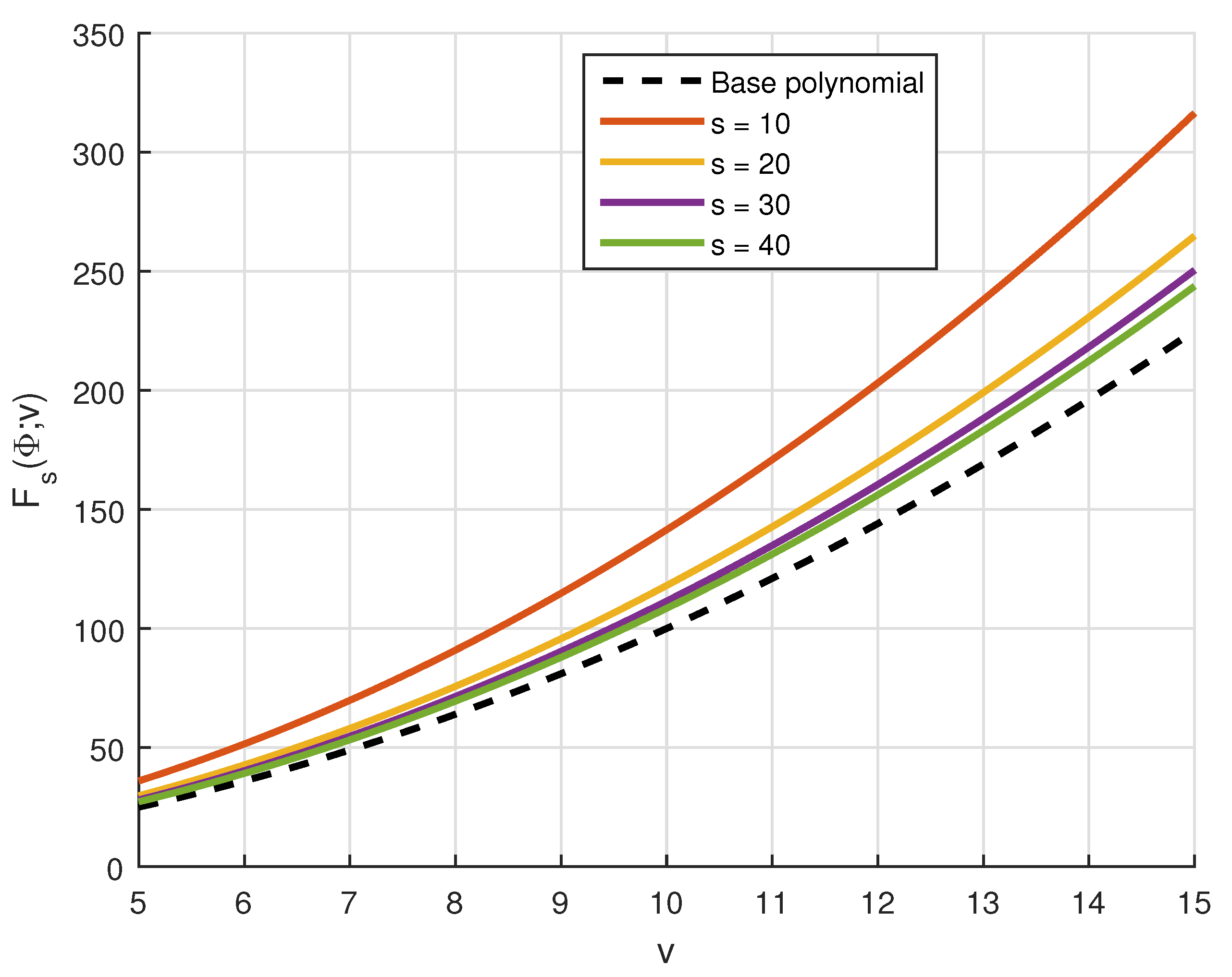
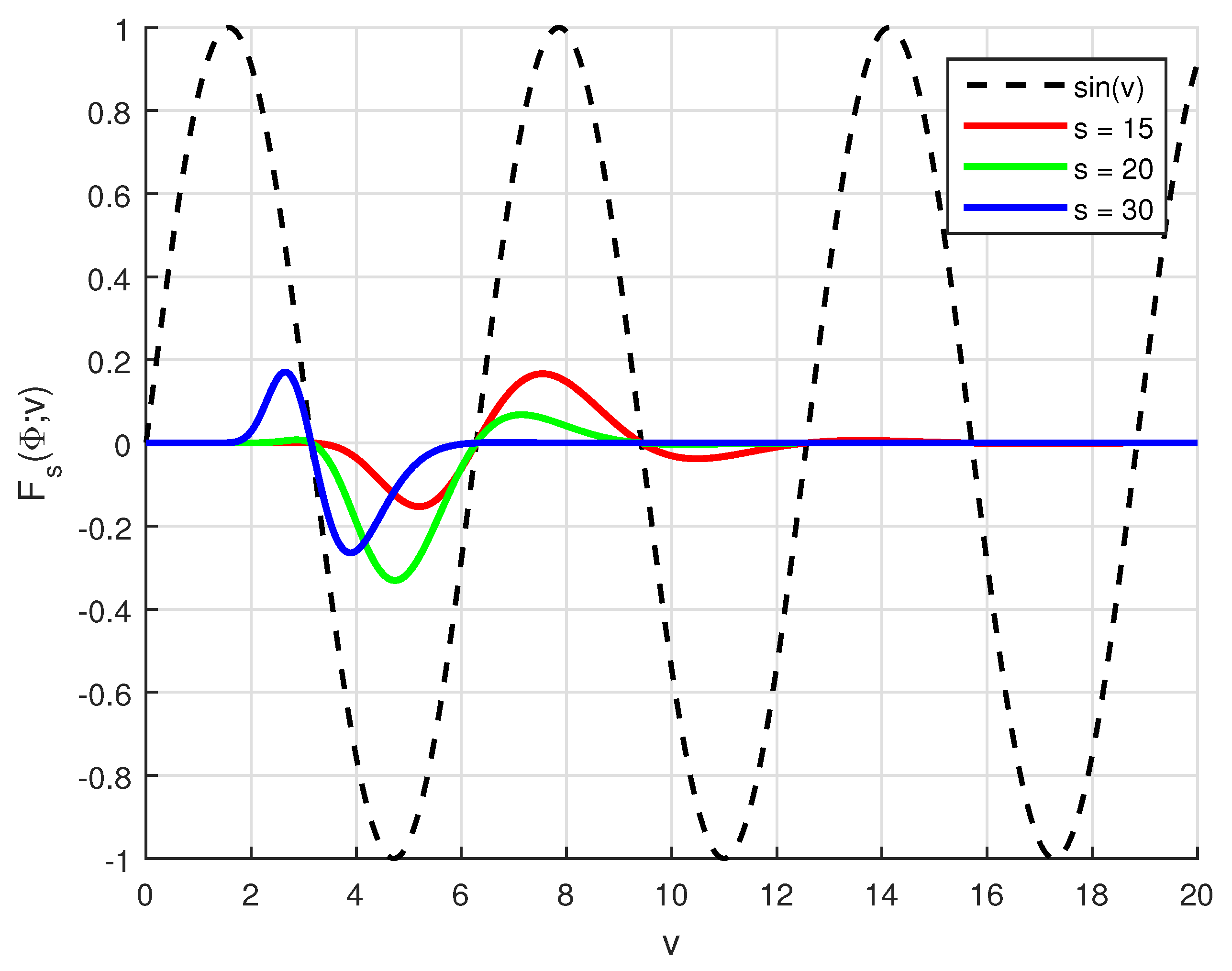
Example 1.

Consider the function $\Phi \left(v\right)=v^2$. Using MATLAB R2015a on a standard HP laptop equipped with an Intel Core i7 processor and 8 GB of RAM, we compute the operator $F_s(\Phi ;v)$ for values of v ranging from 5 to 15, and for distinct values of the parameter s, namely $s=10, 20, 30, 40$. In Figure 1, we present the approximation behavior of the operator for the function $v^2$, which demonstrates how the operator acts on this specific test function. Additionally, we calculated the absolute error between the exact function and its approximation using the same parameters, $|F_s(\Phi ;v)-v^2|$, and the results are depicted in Figure 2 and also provided in

Table 1. Absolute errors for distinct s.

v	$|{\mathit{F}}_{\mathit{s}}(\mathbf{\Phi };\mathit{v})-{\mathit{v}}^2|$ $\mathit{s}=10$	$|{\mathit{F}}_{\mathit{s}}(\mathbf{\Phi };\mathit{v})-{\mathit{v}}^2|$ $\mathit{s}=20$	$|{\mathit{F}}_{\mathit{s}}(\mathbf{\Phi };\mathit{v})-{\mathit{v}}^2|$ $\mathit{s}=30$	$|{\mathit{F}}_{\mathit{s}}(\mathit{\Phi };\mathit{v})-{\mathit{v}}^2|$ $\mathit{s}=40$
5	10.9904	4.7751	3.0479	2.2380
5.0250	11.0945	4.8205	3.0768	2.2592
5.0501	11.1991	4.8660	3.1059	2.2805
5.0751	11.3042	4.9117	3.1351	2.3020
5.1002	11.4098	4.9576	3.1644	2.3235

for the same. This helps illustrate the convergence behavior and accuracy of the operator with respect to the increase in parameter s.

Example 2.

Consider the function $\Phi \left(v\right)=sinv$. Using MATLAB R2015a on a standard HP laptop equipped with an Intel Core i7 processor and 8 GB of RAM, we compute the operator $F_s(\Phi ;v)$ for values of v ranging from 0 to 20, and for distinct values of the parameter s, namely $s=15,20,30$. In Figure 3, we present the approximation behavior of the operator for the function $sinv$, which demonstrates how the operator acts on this specific test function. This helps illustrate the convergence behavior and accuracy of the operator with respect to the increase in parameter s.

7. Conclusions

In this paper, we introduce a sequence of positive linear operators formulated using Frobenius–Euler–Şimşek-type polynomials in integral form. These operators, referred to as Szász–Beta type operators and defined in (4), are constructed to approximate functions defined on Lebesgue measurable spaces. We establish essential estimates to analyze the rate of convergence and the accuracy of approximation. Furthermore, we investigate various aspects of approximation theory, including both local and global results, as well as A-statistical convergence properties. To demonstrate the effectiveness and applicability of the proposed operators, we present several illustrative examples and visualize the results graphically. These examples highlight the practical behavior and confirm the validity of our theoretical findings across different functional settings.

References

- Weierstrass, K. Über die Analytische Darstellbarkeit Sogenannter Willkürlicher Functionen einer Reellen Veränderlichen; Sitzungsberichte der Königlich Preußischen Akademie der Wissenschaften zu Berlin: Berlin, Germany, 1885; Volume 2, pp. 633–639. [Google Scholar]
- Bernstein, S.N. Démonstration du théorème de Weierstrass fondée sur le calcul de probabilités. Commun. Kharkov Math. Soc. 1912, 13, 1–2. [Google Scholar]
- Szász, O. Generalization of Bernstein’s polynomials to the infinite interval. J. Res. Nat. Bur. Stds. 1950, 45, 239–245. [Google Scholar] [CrossRef]
- Özger, F. Weighted statistical approximation properties of univariate and bivariate λ-Kantorovich operators. Filomat 2019, 33, 3473–3486. [Google Scholar] [CrossRef]
- Aslan, R. Approximation by Szász Mirakjan Durrneyer operators based on shape parameter λ. Commun. Fac. Sci. Univ. Ank. Ser. A1 Math. Stat. 2022, 71, 407–421. [Google Scholar] [CrossRef]
- Acu, A.M.; Gonska, H.; Raşa, I. Grüss-type and Ostrowski-type inequalities in approximation theory. Ukr. Math. J. 2011, 63, 843–864. [Google Scholar] [CrossRef]
- Acu, A.M.; Acar, T.; Radu, V.A. Approximation by modified operators. Rev. R. Acad. Ciene. Exactas Fis. Nat. Ser. A Math. RACSAM 2019, 113, 2715–2729. [Google Scholar] [CrossRef]
- Mohiuddine, S.A.; Acar, T.; Alotaibi, A. Construction of a new family of Bernstein-Kantorovich operators. Math. Methods Appl. Sci. 2017, 40, 7749–7759. [Google Scholar] [CrossRef]
- Mohiuddine, S.A.; Ahmad, N.; Özger, F.; Alotaibi, A.; Hazarika, B. Approximation by the parametric generalization of Baskakov–Kantorovich operators linking with Stancu operators. Iran. J. Sci. Technol. Trans. 2021, 45, 593–605. [Google Scholar] [CrossRef]
- Mursaleen, M.; Ansari, K.J.; Khan, A. Approximation properties and error estimation of q-Bernstein shifted operators. Numer. Algorithms 2020, 84, 207–227. [Google Scholar] [CrossRef]
- Mursaleen, M.; Naaz, A.; Khan, A. Improved approximation and error estimations by King type (p, q)-Szász-Mirakjan Kantorovich operators. Appl. Math. Comput. 2019, 348, 2175–2185. [Google Scholar] [CrossRef]
- Khan, A.; Mansoori, M.; Khan, K.; Mursaleen, M. Phillips-type q-Bernstein operators on triangles. J. Funct. Spaces 2021, 2021, 6637893. [Google Scholar] [CrossRef]
- Nasiruzzaman, M. Approximation properties by Szász–Mirakjan operators to bivariate functions via Dunkl analogue. Iran. J. Sci. Technol. Trans. 2021, 45, 259–269. [Google Scholar] [CrossRef]
- Rao, N.; Farid, M.; Ali, R. Study of Szász–Durremeyer-Type Operators Involving Adjoint Bernoulli Polynomials. Mathematics 2024, 12, 3645. [Google Scholar] [CrossRef]
- Rao, N.; Farid, M.; Raiz, M. Symmetric Properties of λ-Szász Operators Coupled with Generalized Beta Functions and Approximation Theory. Symmetry 2024, 16, 1703. [Google Scholar] [CrossRef]
- Rao, N.; Farid, M.; Raiz, M. Approximation Results: Szász– Kantorovich Operators Enhanced by Frobenius–Euler–Type Polynomials. Axioms 2025, 14, 252. [Google Scholar] [CrossRef]
- Rao, N.; Farid, M.; Raiz, M. On the Approximations and Symmetric Properties of Frobenius–Euler–Şimşek Polynomials Connecting Szász Operators. Symmetry 2025, 17, 648. [Google Scholar] [CrossRef]
- Simsek, Y. Applications of constructed new families of generating-type functions interpolating new and known classes of polynomials and numbers. Math. Methods Appl. Sci. 2021, 44, 11245–11268. [Google Scholar] [CrossRef]
- Simsek, Y. On generating functions for the special polynomials. Filomat 2017, 31, 9–16. [Google Scholar] [CrossRef]
- Simsek, Y. Construction of some new families of Apostol-type numbers and polynomials via Dirichlet character and p-adic q-integrals. Turk. J. Math. 2018, 42, 557–577. [Google Scholar] [CrossRef]
- Gadjiev, A.D. The convergence problem for a sequence of positive linear operators on bounded sets and theorems analogous to that of P. P. Korovkin. Dokl. Akad. Nauk SSSR 1974, 218, 1001–1004. [Google Scholar]
- DeVore, R.A.; Lorentz, G.G. Constructive Approximation; Grudlehren der Mathematischen Wissenschaften Fundamental Principales of Mathematical Sciences; Springer: Berlin, Germany, 1993. [Google Scholar]
- Korovkin, P.P. On convergence of linear positive operators in the space of continuous functions. Dokl. Akad. Nauk. SSSR 1953, 90, 961–964. [Google Scholar]
- Shisha, O.; Mond, B. The degree of convergence of linear positive operators. Proc. Nat. Acad. Sci. USA 1968, 60, 1196–1200. [Google Scholar] [CrossRef] [PubMed]
- Lenze, B. On Lipschitz type maximal functions and their smoothness spaces. Nederl Akad Indag Math. 1988, 50, 53–63. [Google Scholar] [CrossRef]
- Gadjiev, A.D. On P. P. Korovkin type theorems. Mat. Zametki 1976, 20, 781–786, reprinted in Transl. in Math. Notes 1978, 5–6, 995–998. [Google Scholar]
- Gadjiev, A.D.; Orhan, C. Some approximation theorems via statistical convergence. Rocky Mt. J. Math. 2007, 32, 129–138. [Google Scholar] [CrossRef]