Reliability Analysis of Improved Type-II Adaptive Progressively Inverse XLindley Censored Data

Abstract

This study offers a newly improved Type-II adaptive progressive censoring with data sampled from an inverse XLindley (IXL) distribution for more efficient and adaptive reliability assessments. Through this sampling mechanism, we evaluate the parameters of the IXL distribution, as well as its reliability and hazard rate features. In the context of reliability, to handle flexible and time-constrained testing frameworks in high-reliability environments, we formulate maximum likelihood estimators versus Bayesian estimates derived via Markov chain Monte Carlo techniques under gamma priors, which effectively capture prior knowledge. Two patterns of asymptotic interval estimates are constructed through the normal approximation of the classical estimates and of the log-transformed classical estimates. On the other hand, from the Markovian chains, two patterns of credible interval estimates are also constructed. A robust simulation study is carried out to compare the classical and Bayesian point estimation methods, along with the four interval estimation methods. This study’s practical usefulness is demonstrated by its analysis of a real-world dataset. The results reveal that both conventional and Bayesian inferential methods function accurately, with the Bayesian outcomes surpassing those of the conventional method.

1. Introduction

In recent years, the use of censored samples to draw inferences about populations of interest has increased in the context of reliability studies and life-testing experiments. This trend may be attributed to advancements in modern technology, which have led to the production of more reliable products. To investigate the reliability of such products, it is not practical for researchers to wait for all items under test to fail. Instead, they can gather information from a portion of these items by terminating the experiment before all failures occur. In this case, the acquired sample is referred to as a censored sample. This approach is highly effective for saving money, time, and human resources. The statistical literature describes various censoring strategies, typically classified as single-stage or multi-stage censoring plans. In single-stage censoring, the experiment concludes after reaching a predetermined number of failures or a specified duration, similar to Type-I and Type-II censoring schemes. In these plans, no withdrawals are permitted before the designated endpoint. On the other hand, multi-stage censoring plans allow for the removal of certain items that are still working from the test at any point, rather than only at the end. One of the most common multi-stage censoring plans is progressive Type-II censoring. For more information, refer to Aggarwala and Balakrishnan [1] and Balakrishnan and Cramer [2]. Several modifications have been introduced to generalize the progressive Type-II censoring plan.

For example, Ng et al. [3] suggested an adaptive Type-II progressive censoring (AT-2PC) scheme which allowed the progressive Type-II censoring plan to be derived as a special case. This procedure allows experimenters to conclude the investigation when the testing time exceeds a predetermined boundary. They also noted that the AT-2PC plan functions efficiently in statistical deductions when the total time of the test is not a considerable issue. However, if the test teams are highly reliable, the testing duration may become too long, causing the AT-2PC plan to fall short of guaranteeing an appropriate overall test length. This scheme has been used in several investigations, including those by Al-Essa et al. [4], Elshahhat and Nassar [5], Lv et al. [6], Dutta et al. [7], Alqasem et al. [8], and Almuhayfith [9]. To address this problem, Yan et al. [10] suggested an improved Type-II adaptive progressive censoring (IT2-APC) plan, which is particularly advantageous when the duration of the test is a critical factor. The IT2-APC plan offers two significant benefits. First, it generalizes several existing plans, including but not limited to the progressive Type-II censoring and AT-2PC plans. Second, it confirms that the experiment ends within a determined time frame. The following is a detailed discussion of how to collect the IT2-APC sample. We assume there are n items undergoing a test with a predetermined number of failures, m. The test follows a progressive censoring pattern, denoted as $\left(S_1,\dots ,S_m\right)$, and involves a pair of threshold times, $T_1$ and $T_2$, where $T_1<T_2$. Let $X_{i:m:n}$ represent the failure time of item $i,i=1,\dots ,m$. After obtaining $X_{1:m:n}$, the researcher randomly selects $S_1$ of the remaining items and removes them from the test. 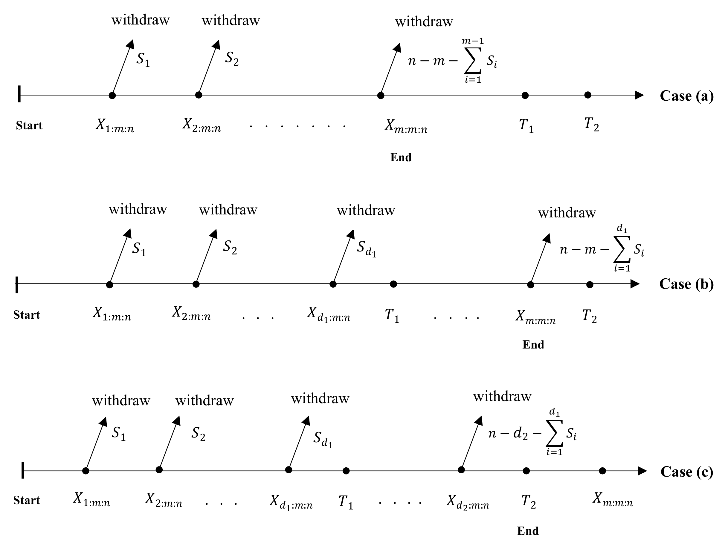Similarly, at $X_{2:m:n}$, $S_2$ of the remaining items are selected and removed from the test, and so on. Under the IT2-APC plan, we can stop the experiment in one of the following three cases:

(a)

If $X_{m:m:n}<T_1$, stop the test at $X_{m:m:n}$. This scenario represents the case of a progressively Type-II censored sample.

(b)

If $T_1<X_{m:m:n}<T_2$, stop the test at $X_{m:m:n}$. In this case, the removal pattern is updated by setting $S_{d_1+1}=\cdots =S_{m-1}=0$, where $d_1$ represents the number of items that failed before $T_1$. This scenario illustrates the case of the AT-2PC sample.

(c)

If $T_2<X_{m:m:n}$, stop the test at $T_2$ with the understanding that the removal pattern is updated by setting $S_{d_1+1}=\cdots =S_{d_2-1}=0$, where $d_2<m$ represents the number of items that failed before $T_2$. After reaching $T_2$, all remaining items $S^{*}=n-d_2-{\sum }_{i=1}^{d_1}{S}_i$ are removed from the test. This scenario illustrates the case of the IT2-APC sample.

Many authors have used the IT2-APC scheme to study estimation concerns for certain lifetime models—for example, the Burr Type-III distribution by Asadi et al. [11], the Weibull distribution by Nassar and Elshahhat [12], a Weibull competing risk model by Elshahhat and Nassar [13], a logistic–exponential distribution by Dutta et al. [14], a Chen distribution by Zhang and Yan [15], an inverted Lomax distribution by Alotaibi et al. [16], a Weibull–exponential distribution by Alotaibi et al. [17], and the Kumaraswamy-G family of distributions by Irfan et al. [18], among others. For an observed IT2-APC sample, $\underline{\mathbf{x}}=(x_1<\cdots <x_{d_1}<T_1<\cdots <x_{d_2}<T_2$), where $x_i$ is the realization of $X_{i:m:n},i=1,\dots ,d_2$, with the progressive censoring scheme $\left(S_1,\dots ,S_{d_1},0,\dots ,0,S^{*}\right)$. As a result, the joint likelihood function of the observed data can be expressed in the following general form:

$$L\left(\underline{\mathbf{x}}\right)=C\prod _{i=1}^{Q_2}f\left(x_i\right)\prod _{i=1}^{Q_1}{\left[1-F\left(x_i\right)\right]}^{S_i}{\left[1-F\left(\tau \right)\right]}^{S^{*}},$$

(1)

where C is a constant, $f(.)$ and $F(.)$ are the probability density function (PDF) and the cumulative distribution function (CDF) of any lifetime model, and the different values of $\tau$, $Q_1$, $Q_2$, and $S^{*}$ are presented in

Table 1. Various cases of $\tau$, $Q_1$, $Q_2$, and $S^{*}$.

Censored Sample	$\mathit{\tau }$	${\mathit{Q}}_1$	${\mathit{Q}}_2$	${\mathit{S}}^{*}$
Progressive Type-II	0	m	m	0
Adaptive Type-II progressive	$x_m$	$d_1$	m	$n-m-{\sum }_{i=1}^{d_1}{S}_i$
Improved Type-II adaptive progressive	$T_2$	$d_1$	$d_2$	$n-d_2-{\sum }_{i=1}^{d_1}{S}_i$

. The detailed experimental procedures for the various cases of the IT2-APC plan are illustrated in Figure 1.

In reliability analyses, it is essential to assume that the population being studied follows a probability distribution that accurately describes its characteristics. In this study, we assume that the population of interest follows the inverse XLindley (IXL) distribution. The IXL distribution, suggested by Beghriche et al. [19], functions as an inverse version of the XLindley (XL) distribution. Let the random variable Y follow the XL distribution. By applying the transformation $X=1/Y$, we conclude that the random variable X follows the IXL distribution. It can be represented as $X\sim \mathrm{IXL}\left(\alpha \right)$, where $\alpha >0$ is a scale parameter. The PDF and the CDF corresponding to the random variable X are written as

$$f(x;\alpha )={\displaystyle \frac{{\alpha }^2}{{(1+\alpha )}^2{x}^3}}[1+(2+\alpha )x]e^{-{\displaystyle \frac{\alpha }{x}}},x>0,\alpha >0$$

(2)

and

$$F(x;\alpha )=\left[1+{\displaystyle \frac{\alpha }{x{(1+\alpha )}^2}}\right]e^{-{\displaystyle \frac{\alpha }{x}}},$$

(3)

respectively.

Beghriche et al. [19] investigated the key characteristics of the IXL distribution and noted that its hazard rate function (HRF) can be used to model data exhibiting an upside-down bathtub shape. The reliability function (RF) and the HRF, at time point $t>0$, of the IXL distribution can be expressed, respectively, as

$$R(t;\alpha )=1-\left[1+{\displaystyle \frac{\alpha }{t{(1+\alpha )}^2}}\right]e^{-{\displaystyle \frac{\alpha }{t}}},t>0$$

(4)

and

$$h(t;\alpha )={\displaystyle \frac{{\alpha }^2[1+(2+\alpha )t]e^{-\frac{\alpha }{t}}}{t^2\left[t{(1+\alpha )}^2\left(1-e^{-\frac{\alpha }{t}}\right)-\alpha e^{-\frac{\alpha }{t}}\right]}}.$$

(5)

We are motivated to complete the current work for many reasons: (1) The significance of the IXL distribution in modeling reliability data with heavy-tailed behavior and non-monotonic hazard rates. These characteristics make it particularly suitable for high-reliability systems where the failure modes evolve over time, such as in electronic components or medical survival data. Unlike traditional inverted distributions, as shown later in the data analysis section, we compared the IXL distribution and several inverted lifetime models, specifically thirteen inverted models, encompassing both classical inverted models and recently introduced inverted distributions. The findings revealed that the IXL distribution offers a superior fit based on several goodness-of-fit criteria. (2) The IT2-APC scheme offers notable flexibility, which has been recognized in recent studies for its effectiveness in balancing the test duration and estimation accuracy, particularly for highly reliable products. For example, Yan et al. [10] showed that the IT2-APC scheme shortens the testing time by adaptively removing units based on pre-specified thresholds, $T_1$ and $T_2$. This approach has proven more efficient than traditional progressive Type-II censoring or AT-2PC plan failures. Such adaptability makes the IT2-APC scheme well suited to practical reliability applications, where extended testing periods are often infeasible. While recent studies have explored censored inferences for other inverted distributions, such as the inverted Weibull (IW) distribution by Kazemi and Azizpoor [20] and the inverted Lindley (IL) distribution by Abushal and AL-Zaydi [21], no research has yet addressed the IXL distribution under the IT2-APC scheme or any other censoring framework. Beghriche et al. [19] focused on classical estimation for the IXL distribution but did not consider Bayesian inference, interval estimation, or analyses of the RF and the HRF. Moreover, comparisons with competing inverted models in terms of the goodness-of-fit have not been investigated, limiting the ability of practitioners to justify the use of the IXL distribution in reliability modeling.

This study aims to address several unresolved challenges in the field of reliability testing and statistical estimation. Specifically, it focuses on evaluating the parameters of the IXL distribution, including its RF and HRF, under the IT2-APC scheme, which is crucial for high-reliability testing scenarios. A significant gap exists in the current literature regarding Bayesian estimation methods and the construction of both ACIs and credible intervals for the IXL distribution. Moreover, although the IXL distribution is often described as flexible, there is a lack of empirical comparisons with other inverted distributions. This highlights the need for a comprehensive comparative analysis to validate the IXL model’s performance and justify its adoption in real-world reliability applications. In this study, we consider two estimation methods, namely (1) maximum likelihood estimation, as a classical method, and (2) the Bayesian estimation method. These methods are applied to estimating both the model parameters and the two reliability indicators, namely the RF and the HRF. Collectively, these three quantities will be referred to as the unknown parameters. Accordingly, the objectives of the study can be summarized as follows:

1.

Estimate the unknown parameters of the model using both maximum likelihood and Bayesian estimation methods, providing a comprehensive comparison through point estimates, two approximate confidence intervals (ACIs), and two credible intervals;

2.

Assess the accuracy and efficiency of the proposed estimation methods under the IT2-APC scheme through an extensive simulation study;

3.

Compare the IXL distribution with several competing inverted lifetime models to evaluate and demonstrate its superior performance using various goodness-of-fit measures;

4.

Validate the practical applicability and relevance of the IXL model and the IT2-APC plan by analyzing a real-world reliability dataset, thereby illustrating their utility in real-life reliability strategies.

The rest of this study is classified as follows: Section 2 investigates the classical point and interval estimates of the unknown parameters. The Bayes point and credible intervals of the various unknown parameters are illustrated in Section 3. Section 4 shows the simulation setup, as well as the numerical findings. One real dataset is explored in Section 5. Section 6 concludes this paper.

2. Classical Point and Interval Estimations

This section presents the maximum likelihood estimates (MLEs) of the unknown parameters $\alpha$, the RF, and the HRF. Additionally, two ACIs are provided: the first uses the normal approximation of the MLEs, designated as ACIs-NA, and the second uses the normal approximation of the log-transformed MLEs, designated as ACIs-NL. A key aspect in calculating the interval estimates for the RF and the HRF is determining the variance in their MLEs. This study uses the delta method to estimate these necessary variances.

Take an IT2-APC sample from the IXL population, denoted by $\underline{\mathbf{x}}=(x_1<\cdots <x_{d_1}<T_1<\cdots <x_{d_2}<T_2$), with the removal scheme $\left(S_1,\dots ,S_{d_1},0,\dots ,0,S^{*}\right)$. Then, after ignoring the constant terms, the likelihood function can be formulated using (1)–(3) as

$$\begin{array}{ccc}\hfill L\left(\alpha \right|\underline{\mathbf{x}})& =& {\left({\displaystyle \frac{\alpha }{1+\alpha }}\right)}^{2Q_2}exp\left\{-\alpha \sum _{i=1}^{Q_2}{x}_i^{-1}+\sum _{i=1}^{Q_2}log[1+(2+\alpha )x_i]\right\}\hfill \\ & \times & exp\left\{\sum _{i=1}^{Q_1}{S}_{i}log[1-\psi (x_i;\alpha )]+S^{*}log[1-\psi (\tau ;\alpha )]\right\},\hfill \end{array}$$

(6)

where $\psi (x_i;\alpha )=\left[1+{\displaystyle \frac{\alpha }{x_i{(1+\alpha )}^2}}\right]e^{-{\displaystyle \frac{\alpha }{x_i}}}$. The natural logarithm of (6), denoted by $l(.)$, follows

$$\begin{array}{ccc}\hfill l\left(\alpha \right|\underline{\mathbf{x}})& =& 2Q_{2}log\left({\displaystyle \frac{\alpha }{1+\alpha }}\right)-\alpha \sum _{i=1}^{Q_2}{x}_i^{-1}+\sum _{i=1}^{Q_2}log[1+(2+\alpha )x_i]+\sum _{i=1}^{Q_1}{S}_{i}log[1-\psi (x_i;\alpha )]\hfill \\ & +& S^{*}log[1-\psi (\tau ;\alpha )].\hfill \end{array}$$

(7)

After differentiating (7) with respect to $\alpha$ and setting the result equal to zero, we obtain the following nonlinear normal equation:

$$\begin{array}{c}\hfill {\displaystyle \frac{dl\left(\alpha \right|\underline{\mathbf{x}})}{d\alpha }}={\displaystyle \frac{2Q_2}{\alpha (1+\alpha )}}-\sum _{i=1}^{Q_2}{x}_i^{-1}+\sum _{i=1}^{Q_2}{\displaystyle \frac{x_i}{1+(2+\alpha )x_i}}+\sum _{i=1}^{Q_1}{\displaystyle \frac{S_i{\psi }_1(x_i;\alpha )}{1-\psi (x_i;\alpha )}}+{\displaystyle \frac{S^{*}{\psi }_1(\tau ;\alpha )}{1-\psi (\tau ;\alpha )}}=0,\end{array}$$

(8)

where

$${\psi }_1(x_i;\alpha )={\displaystyle \frac{\alpha e^{-\frac{\alpha }{x_i}}\left[1+\alpha +x_i(4+3\alpha +{\alpha }^2)\right]}{x_i^2{(1+\alpha )}^3}}.$$

It is noted that the MLE of the unknown parameter $\alpha$, denoted as $\widehat{\alpha }$, cannot be obtained explicitly because of the complex form of the resulting normal equation. To address this issue, we use the Newton–Raphson method to compute the MLE $\widehat{\alpha }$ numerically from (8). After obtaining the MLE $\widehat{\alpha }$, we apply the invariance property of the MLE to computing the MLEs for the RF and the HRF. These estimates can be derived based on (4) and (5), respectively, as follows:

$$\widehat{R}\left(t\right)=1-\left[1+{\displaystyle \frac{\widehat{\alpha }}{t{(1+\widehat{\alpha })}^2}}\right]e^{-{\displaystyle \frac{\widehat{\alpha }}{t}}}$$

and

$$\widehat{h}\left(t\right)={\displaystyle \frac{{\widehat{\alpha }}^2[1+(2+\widehat{\alpha })t]e^{-\frac{\widehat{\alpha }}{t}}}{t^2\left[t{(1+\widehat{\alpha })}^2\left(1-e^{-\frac{\widehat{\alpha }}{t}}\right)-\widehat{\alpha }{e}^{-{\displaystyle \frac{\widehat{\alpha }}{t}}}\right]}}.$$

In addition to calculating the point estimates of the unknown parameters, it is important to examine their interval estimates. The normal approximation of the MLE allows us to obtain such intervals.

In this study, we estimate the variance in the MLE $\widehat{\alpha }$ by inverting the observed Fisher information matrix. To perform this, we first compute the second-order derivative of the log-likelihood function in (7) as

$$\begin{array}{ccc}\hfill {\displaystyle \frac{d^{2}l\left(\alpha \right|\underline{\mathbf{x}})}{d{\alpha }^2}}& =& -{\displaystyle \frac{2Q_2(1+2\alpha )}{{\alpha }^2{(1+\alpha )}^2}}-\sum _{i=1}^{Q_2}{\displaystyle \frac{x_i^2}{{[1+(2+\alpha )x_i]}^2}}+\sum _{i=1}^{Q_1}{\displaystyle \frac{S_i{\psi }_2(x_i;\alpha )}{{[1-\psi (x_i;\alpha )]}^2}}+{\displaystyle \frac{S^{*}{\psi }_2(\tau ;\alpha )}{{[1-\psi (\tau ;\alpha )]}^2}},\hfill \end{array}$$

(9)

where

$$\begin{array}{ccc}\hfill {\psi }_2(x_i;\alpha )& =& [\psi (x_i;\alpha )-1]\left[{\displaystyle \frac{\psi (x_i;\alpha )}{x_i^2}}+{\displaystyle \frac{2e^{-\frac{\alpha }{x_i}}({\alpha }^2+\alpha x_i-2x_i-1)}{x_i^2{(1+\alpha )}^4}}\right]\hfill \\ & -& {\left[{\displaystyle \frac{\psi (x_i;\alpha )}{x_i}}+{\displaystyle \frac{(\alpha -1)e^{-\frac{\alpha }{x_i}}}{x_i{(1+\alpha )}^3}}\right]}^2.\hfill \end{array}$$

(10)

Then, we can obtain the estimated variance in the MLE $\widehat{\alpha }$ as

$${\widehat{var}}_1={\left[-{\displaystyle \frac{d^{2}l\left(\alpha \right|\underline{\mathbf{x}})}{d{\alpha }^2}}\right]}^{-1},$$

(11)

where ${\widehat{var}}_1$ in (11) is computed at $\widehat{\alpha }$.

On the other hand, the delta method is applied to obtain the estimated variances for the MLEs of the RF and the HRF, denoted by ${\widehat{var}}_2$ and ${\widehat{var}}_3$, respectively. According to this approach, the estimated variances can be computed as

$${\widehat{var}}_2\approx \left[{\widehat{\Delta }}_1{\widehat{var}}_1{\widehat{\Delta }}_1^{\top }\right]\mathrm{and}{\widehat{var}}_3\approx \left[{\widehat{\Delta }}_2{\widehat{var}}_1{\widehat{\Delta }}_2^{\top }\right],$$

where

$${\widehat{\Delta }}_1={\psi }_1(t;\widehat{\alpha })$$

and

$$\begin{array}{ccc}\hfill {\widehat{\Delta }}_2& =& -{\displaystyle \frac{\widehat{\alpha }{e}^{-\frac{\widehat{\alpha }}{t}}[\widehat{\alpha }t(\widehat{\alpha }-3t+2)+\widehat{\alpha }-2t(2t+1)]}{t\widehat{\phi }}}+{\displaystyle \frac{t^2{\widehat{\alpha }}^2{e}^{-\frac{\widehat{\alpha }}{t}}[1+t(2+\widehat{\alpha })]}{{\widehat{\phi }}^2}}\hfill \\ & \times & \left\{e^{-{\displaystyle \frac{\widehat{\alpha }}{t}}}\left[1-{(1+\widehat{\alpha })}^2-{\displaystyle \frac{\widehat{\alpha }}{t}}\right]+2t(1+\widehat{\alpha })\left(e^{-{\displaystyle \frac{\widehat{\alpha }}{t}}}-1\right)\right\},\hfill \end{array}$$

where $\widehat{\phi }=t^2\left[t{(1+\widehat{\alpha })}^2\left(1-e^{-{\displaystyle \frac{\widehat{\alpha }}{t}}}\right)-\widehat{\alpha }{e}^{-{\displaystyle \frac{\widehat{\alpha }}{t}}}\right]$.

Then, at a $100(1-ϵ)\%$ confidence level, the ACIs-NA of the unknown parameters $\alpha$, the RF, and the HRF can be computed as

$$\widehat{\alpha }\pm z_{ϵ/2}\sqrt{{\widehat{var}}_1},\widehat{R}\left(t\right)\pm z_{ϵ/2}\sqrt{{\widehat{var}}_2}\mathrm{and}\widehat{h}\left(t\right)\pm z_{ϵ/2}\sqrt{{\widehat{var}}_3},$$

where $z_{ϵ/2}$ is the upper ${(ϵ/2)}^{th}$ percentile point obtained from the standard normal distribution. In addition, the $100(1-ϵ)\%$ ACIs-NL of the various unknown parameters can be obtained as

$$\widehat{\alpha }\times exp\left[\pm z_{ϵ/2}{\displaystyle \frac{\sqrt{{\widehat{var}}_1}}{\widehat{\alpha }}}\right],\widehat{R}\left(t\right)\times exp\left[\pm z_{ϵ/2}{\displaystyle \frac{\sqrt{{\widehat{var}}_2}}{\widehat{R}\left(t\right)}}\right]\mathrm{and}\widehat{h}\left(t\right)\times exp\left[\pm z_{ϵ/2}{\displaystyle \frac{\sqrt{{\widehat{var}}_3}}{\widehat{h}\left(t\right)}}\right].$$

To evaluate both the point and $100(1-ϵ)\%$ interval frequentist estimates of $\alpha$, $R\left(t\right)$, or $h\left(t\right)$, we recommend implementing the ’$\mathsf{maxLik}$’ package, proposed by Henningsen and Toomet [22].

Theorem 1.

For the IXL distribution, at least one $\widehat{\alpha }\in (0,\infty )$ exists satisfying the score equation ${\displaystyle \frac{dl\left(\alpha \right|\underline{\mathbf{x}})}{d\alpha }}=0$, implying the existence of an MLE.

Proof. 

Consider the score function $s\left(\alpha \right)={\displaystyle \frac{dl\left(\alpha \right|\underline{\mathbf{x}})}{d\alpha }}$. We show that $s\left(\alpha \right)=0$ has a solution in $(0,\infty )$.

As $\alpha \to 0^{+}$,

• ${\displaystyle \frac{2Q_2}{\alpha (1+\alpha )}}\approx {\displaystyle \frac{2Q_2}{\alpha }}\to +\infty$.
• $-{\sum }_{i=1}^{Q_2}{x}_i^{-1}=-C<0$, where $C={\sum }_{i=1}^{Q_2}{x}_i^{-1}$.
• ${\sum }_{i=1}^{Q_2}{\displaystyle \frac{x_i}{1+(2+\alpha )x_i}}\to {\sum }_{i=1}^{Q_2}{\displaystyle \frac{x_i}{1+2x_i}}>0$.
• ${\psi }_1(x_i;\alpha )\approx {\displaystyle \frac{\alpha (1+4x_i)}{x_i^2}}\to 0$, $\psi (x_i;\alpha )\to 1$, so ${\displaystyle \frac{{\psi }_1(x_i;\alpha )}{1-\psi (x_i;\alpha )}}\to 0^{+}$ if $1-\psi (x_i;\alpha )>0$. Thus, ${\sum }_{i=1}^{Q_1}{\displaystyle \frac{S_i{\psi }_1(x_i;\alpha )}{1-\psi (x_i;\alpha )}}\to 0$, similarly for $\tau$. Hence, $s\left(\alpha \right)\to +\infty$.

As $\alpha \to \infty$,

• ${\displaystyle \frac{2Q_2}{\alpha (1+\alpha )}}\to 0^{+}$.
• ${\sum }_{i=1}^{Q_2}{\displaystyle \frac{x_i}{1+(2+\alpha )x_i}}\approx {\displaystyle \frac{1}{\alpha }}\to 0$.
• ${\psi }_1(x_i;\alpha )\approx {\displaystyle \frac{1}{x_i}}{e}^{-\alpha /x_i}\to 0$, $\psi (x_i;\alpha )\to 0$, so ${\displaystyle \frac{{\psi }_1(x_i;\alpha )}{1-\psi (x_i;\alpha )}}\to 0$. Thus, $s\left(\alpha \right)\to -C<0$.

Since $s\left(\alpha \right)$ is continuous ($\psi$, ${\psi }_1$ are continuous, $1-\psi (x_i;\alpha )=F(x_i;\alpha )>0$), and $s\left(\alpha \right)\to +\infty$ as $\alpha \to 0^{+}$, $s\left(\alpha \right)\to -C<0$ as $\alpha \to \infty$, $\widehat{\alpha }\in (0,\infty )$ exists such that $s\left(\widehat{\alpha }\right)=0$. The second derivative (see Theorem 2.2) confirms this is a maximum. □

Theorem 2.

For the IXL distribution, under the conditions in Theorem 2.1, the MLE $\widehat{\alpha }\in (0,\infty )$ is unique.

Proof. 

To show that the MLE is unique, we prove the log-likelihood is strictly concave, i.e., ${\displaystyle \frac{d^{2}l\left(\alpha \right|\underline{\mathbf{x}})}{d{\alpha }^2}}<0$. Let $\acute{s}\left(\alpha \right)={\displaystyle \frac{d^{2}l\left(\alpha \right|\underline{\mathbf{x}})}{d{\alpha }^2}}$. Then, one can see the following from (9):

1.

The first term in $\acute{s}\left(\alpha \right)$$-{\displaystyle \frac{2Q_2(1+2\alpha )}{{\alpha }^2{(1+\alpha )}^2}}<0$.

2.

The second term $-{\sum }_{i=1}^{Q_2}{\displaystyle \frac{x_i^2}{{[1+(2+\alpha )x_i]}^2}}<0$.

3.

For the censoring terms in $\acute{s}\left(\alpha \right)$, one can easily see from ${\psi }_2(x_i;\alpha )$ in (10) that $\psi (x_i;\alpha )-1=-F(x_i;\alpha )<0$ and the squared term in ${\psi }_2(x_i;\alpha )$ is non-positive. Let $K={\displaystyle \frac{\psi (x_i;\alpha )}{x_i^2}}+{\displaystyle \frac{2e^{-\frac{\alpha }{x_i}}({\alpha }^2+\alpha x_i-2x_i-1)}{x_i^2{(1+\alpha )}^4}}$. The first part in K is positive. The sign of the second part depends on $p\left(\alpha \right)={\alpha }^2+\alpha x_i-2x_i-1$. It is simple to see that $p\left(\alpha \right)>0$ if $\alpha >{\alpha }_0=-x_i+\sqrt{x_i^2+4(2x_i+1)}$, and $p\left(\alpha \right)<0$ for $\alpha <{\alpha }_0$. 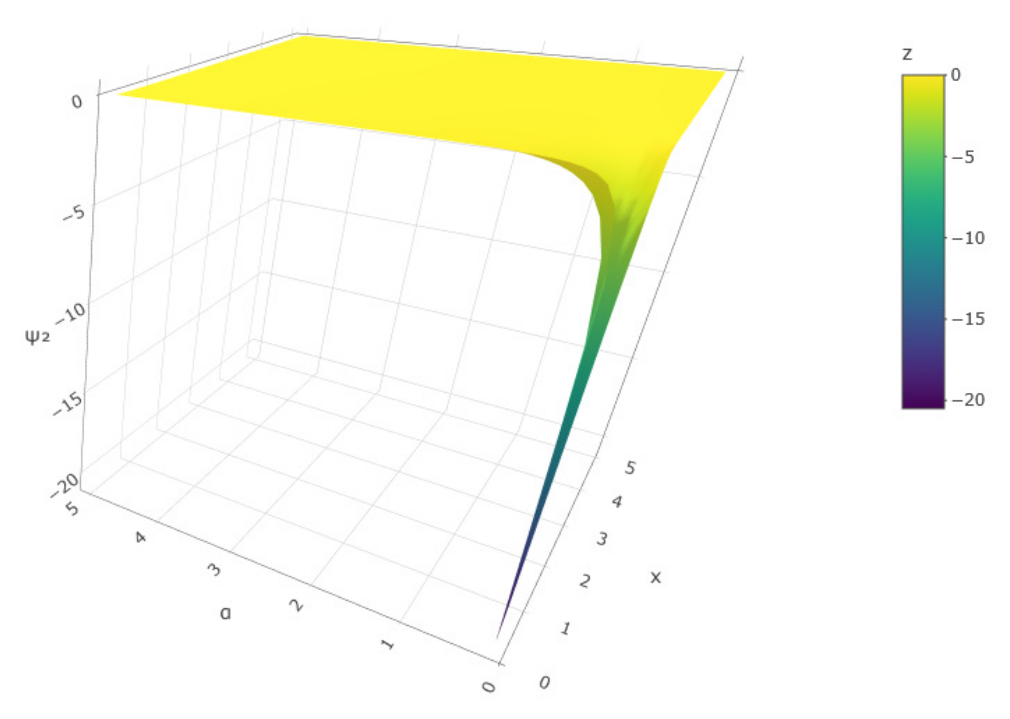As shown in Figure 2, the function ${\psi }_2(x_i;\alpha )$ is always negative, which is due to the dominance of the positive term in K and the squared term in ${\psi }_2(x_i;\alpha )$.

Thus, $\acute{s}\left(\alpha \right)<0$, implying strict concavity. Hence, $s\left(\alpha \right)$ is strictly decreasing and has a unique root, and $\widehat{\alpha }$ is the unique MLE. □

3. Bayesian Point and Interval Estimations

In the field of reliability studies, the ability to integrate prior knowledge is highly advantageous. It enables us to integrate existing knowledge or thoughts about the unknown parameters into the investigation. This inclusion of prior knowledge serves as a foundation for a different type of parametric inference known as Bayesian inference, which has garnered considerable attention as a strong and useful option for frequent estimation approaches. This section focuses on the Bayesian estimation of the unknown parameters of the IXL distribution using the IT2-APC sample. We analyze the point estimations for the various parameters using the squared error loss function. This loss function is widely adopted in Bayesian analyses because of its simplicity and analytical convenience. Specifically, it leads to a closed-form solution for the Bayes estimator, which corresponds to the posterior mean. In the context of reliability studies, the symmetric nature of the squared error loss function ensures that both overestimation and underestimation are treated equally. This property is especially valuable in practical applications such as maintenance scheduling and risk evaluation, where balanced and unbiased parameter estimates are essential. Additionally, we explore two types of Bayesian interval estimates: Bayes credible intervals (BCIs) and highest posterior density (HPD) credible intervals.

To begin with the Bayesian estimation, we need to represent our knowledge of the unknown parameter $\alpha$ through its prior distribution. One common approach is to use the conjugate prior distribution. However, by examining the likelihood function in (6), it becomes clear that there is no conjugate prior available for the unknown parameter $\alpha$. In this case, we take advantage of the flexibility of the gamma distribution and use it as a prior distribution for $\alpha$, expressed in the following form:

$$\pi \left(\alpha \right)\propto {\alpha }^{a-1}exp(-b\alpha ),\alpha >0,a,b>0.$$

(12)

The gamma prior is employed in our Bayesian investigation for several critical reasons: (1) The gamma prior distribution shows considerable flexibility, as it can take various shapes, e.g., exponential, right-skewed, or approximately symmetric, contingent upon its shape parameter. This inherent flexibility facilitates the substantial incorporation of prior knowledge regarding the unknown parameter of interest. (2) Given that the unknown parameter of the IXL distribution is non-negative, the gamma prior distribution constitutes a natural choice, as it is solely determined for positive values. This feature guarantees that the prior knowledge conforms to the physical limitation associated with the unknown parameter. (3) The hyper-parameters of the gamma prior distribution (shape and scale) can be intuitively interpreted in relation to prior knowledge, such as the prior mean and variance, thereby facilitating the specification and illustration of the prior settings. (4) The gamma prior distribution is broadly employed in Bayesian reliability investigations due to its compatibility with lifetime data and capability to deliver powerful and interpretable results. (5) Furthermore, it does not introduce additional complexity into the posterior distribution or computational challenges, particularly when employing the MCMC methods. Given the observed IT2-APC data $\underline{\mathbf{x}}$, the posterior distribution of the unknown parameter $\alpha$ can be expressed as given, after combining the likelihood function in (6) with the prior distribution in (12):

$$\begin{array}{ccc}\hfill g\left(\alpha \right|\underline{\mathbf{x}})& =& {\displaystyle \frac{{\alpha }^{2Q_2+a-1}}{\mathrm{\Lambda }{(1+\alpha )}^{2Q_2}}}exp\left\{-\alpha \left(\sum _{i=1}^{Q_2}{x}_i^{-1}+b\right)+\sum _{i=1}^{Q_2}log[1+(2+\alpha )x_i]\right\}\hfill \\ & \times & exp\left\{\sum _{i=1}^{Q_1}{S}_{i}log[1-\psi (x_i;\alpha )]+S^{*}log[1-\psi (\tau ;\alpha )]\right\},\hfill \end{array}$$

(13)

where $\mathrm{\Lambda }$ is defined as

$$\begin{array}{c}\hfill \mathrm{\Lambda }={\int }_0^{\infty }\pi \left(\alpha \right)g\left(\alpha \right|\underline{\mathbf{x}})d\alpha .\end{array}$$

In light of the posterior distribution in (13), we can write the Bayes estimator of the unknown parameter $\alpha$ under the squared error loss function as

$$\begin{array}{ccc}\hfill \tilde{\alpha }& =& {\int }_0^{\infty }\alpha g\left(\alpha \right|\underline{\mathbf{x}})d\alpha \hfill \\ & =& {\int }_0^{\infty }{\displaystyle \frac{{\alpha }^{2Q_2+a}}{\mathrm{\Lambda }{(1+\alpha )}^{2Q_2}}}exp\left\{-\alpha \left(\sum _{i=1}^{Q_2}{x}_i^{-1}+b\right)+\sum _{i=1}^{Q_2}log[1+(2+\alpha )x_i]\right\}\hfill \\ & \times & exp\left\{\sum _{i=1}^{Q_1}{S}_{i}log[1-\psi (x_i;\alpha )]+S^{*}log[1-\psi (\tau ;\alpha )]\right\}d\alpha .\hfill \end{array}$$

(14)

Similarly, the Bayes estimators of the RF and the HRF can be obtained using (13), respectively, as

$$\begin{array}{ccc}\hfill \tilde{R}\left(t\right)& =& {\int }_0^{\infty }{\displaystyle \frac{R(t;\alpha ){\alpha }^{2Q_2+a-1}}{\mathrm{\Lambda }{(1+\alpha )}^{2Q_2}}}exp\left\{-\alpha \left(\sum _{i=1}^{Q_2}{x}_i^{-1}+b\right)+\sum _{i=1}^{Q_2}log[1+(2+\alpha )x_i]\right\}\hfill \\ & \times & exp\left\{\sum _{i=1}^{Q_1}{S}_{i}log[1-\psi (x_i;\alpha )]+S^{*}log[1-\psi (\tau ;\alpha )]\right\}d\alpha \hfill \end{array}$$

(15)

and

$$\begin{array}{ccc}\hfill \tilde{h}\left(t\right)& =& {\int }_0^{\infty }{\displaystyle \frac{h(t;\alpha ){\alpha }^{2Q_2+a-1}}{\mathrm{\Lambda }{(1+\alpha )}^{2Q_2}}}exp\left\{-\alpha \left(\sum _{i=1}^{Q_2}{x}_i^{-1}+b\right)+\sum _{i=1}^{Q_2}log[1+(2+\alpha )x_i]\right\}\hfill \\ & \times & exp\left\{\sum _{i=1}^{Q_1}{S}_{i}log[1-\psi (x_i;\alpha )]+S^{*}log[1-\psi (\tau ;\alpha )]\right\}d\alpha ,\hfill \end{array}$$

(16)

where $R(t;\alpha )$ and $h(t;\alpha )$ are as defined in (4) and (5), respectively. It is evident that obtaining the Bayes estimators in (14)–(16) for the various parameters is challenging due to the complex form of the posterior distribution. To address this issue and obtain the necessary estimates, we use the Markov chain Monte Carlo (MCMC) technique to generate random samples from the posterior distribution in (13). We then utilize these samples, along with the squared error loss function, to compute the Bayes estimates for $\alpha$, the RF, and the HRF. The BCIs and the HPD credible intervals can be also obtained in this case.

To implement the MCMC technique, it is essential to assess whether the posterior distribution of the random variable $\alpha$ aligns with any well-known distribution. This evaluation is crucial for determining the appropriate MCMC algorithm to use. It is evident from (13) that the posterior distribution does not correspond to any well-known statistical distribution. Therefore, we will utilize the Metropolis–Hastings (MH) algorithm to acquire the necessary samples from the posterior distribution (13). To acquire samples using the M-H algorithm, we utilize the normal distribution as a proposal density. The following steps are used to generate samples from the posterior distribution in (13):

Step 1.

Set $j=1$ and put ${\alpha }^{\left(0\right)}=\widehat{\alpha }$, where $\widehat{\alpha }$ is the MLE of $\alpha$.

Step 2.

Simulate a candidate ${\alpha }^{\prime }$ from $N[{\alpha }^{(j-1)},{\widehat{var}}_1]$.

Step 3.

Compute the acceptance ratio:

$$\vartheta =min\left[1,{\displaystyle \frac{g\left({\alpha }^{\prime }\right|\underline{\mathbf{x}})}{g\left({\alpha }^{(j-1)}\right|\underline{\mathbf{x}})}}\right].$$

Step 4.

Simulate u from the unit uniform distribution.

Step 5.

Take the candidate by setting ${\alpha }^{\left(j\right)}={\alpha }^{\prime }$ if $u\le \vartheta$; otherwise, set ${\alpha }^{\left(j\right)}={\alpha }^{(j-1)}$.

Step 6.

Obtain the RF and the HRF as

$$R^{\left(j\right)}=1-\left[1+{\displaystyle \frac{{\alpha }^{\left(j\right)}}{t{(1+{\alpha }^{\left(j\right)})}^2}}\right]e^{-{\displaystyle \frac{{\alpha }^{\left(j\right)}}{t}}}$$

and

$$h^{\left(j\right)}={\displaystyle \frac{{\left[{\alpha }^{\left(j\right)}\right]}^2[1+(2+{\alpha }^{\left(j\right)})t]e^{-\frac{{\alpha }^{\left(j\right)}}{t}}}{t^2\left[t{(1+{\alpha }^{\left(j\right)})}^2\left(1-e^{-\frac{{\alpha }^{\left(j\right)}}{t}}\right)-{\alpha }^{\left(j\right)}{e}^{-\frac{{\alpha }^{\left(j\right)}}{t}}\right]}}.$$

Step 7.

Set $j=j+1$.

Step 8.

Repeat the approach from steps 2 to 7, M times.

Step 9.

Use the generated samples to construct the sequence

$$\left\{{\alpha }^{\left(j\right)},R^{\left(j\right)},h^{\left(j\right)}\right\},j=1,\dots ,M.$$

Based on the squared error loss function, the Bayes estimates of $\alpha$, the RF, and the HRF can be computed, after a burn-in period B, respectively, as

$$\tilde{\alpha }={\displaystyle \frac{1}{\overline{M}}}{\sum }_{j=B+1}^M{\alpha }^{\left(j\right)},\tilde{R}\left(t\right)={\displaystyle \frac{1}{\overline{M}}}{\sum }_{j=B+1}^M{R}^{\left(j\right)}\mathrm{and}\tilde{h}\left(t\right)={\displaystyle \frac{1}{\overline{M}}}{\sum }_{j=B+1}^M{h}^{\left(j\right)},$$

where $\overline{M}=M-B$. On the other hand, to obtain both the BCIs and the HPD credible intervals, we first sort the sequence $\left\{{\alpha }^{\left(j\right)},R^{\left(j\right)},h^{\left(j\right)}\right\},j=B+1,\dots ,M$ as $\left\{{\alpha }_{(B+1)}<\cdots <{\alpha }_{\left(M\right)}\right\}$, $\left\{R_{(B+1)}<\cdots <R_{\left(M\right)}\right\}$, and $\left\{h_{(B+1)}<\cdots <h_{\left(M\right)}\right\}$. Thus, the $100(1-ϵ)\%$ BCIs for $\alpha$, the RF, and the HRF are as follows:

$$\left\{{\alpha }_{\left(0.5ϵ\overline{M}\right)},{\alpha }_{\left((1-0.5ϵ)\overline{M}\right)}\right\},\left\{R_{\left(0.5ϵ\overline{M}\right)},R_{\left((1-0.5ϵ)\overline{M}\right)}\right\}\mathrm{and}\left\{h_{\left(0.5ϵ\overline{M}\right)},h_{\left((1-0.5ϵ)\overline{M}\right)}\right\},$$

respectively. In addition, the $100(1-\tau )\%$ HPD credible intervals of $\alpha$, the RF, and the HRF are given by

$$\left\{{\alpha }_{\left(j^{*}\right)},{\alpha }_{\left(j^{*}+\left(1-ϵ\right)\overline{M}\right)}\right\},\left\{R_{\left(j^{*}\right)},R_{\left(j^{*}+\left(1-ϵ\right)\overline{M}\right)}\right\}\mathrm{and}\left\{h_{\left(j^{*}\right)},h_{\left(j^{*}+\left(1-ϵ\right)\overline{M}\right)}\right\},$$

respectively, while $j^{*}=B+1,\dots ,M$ is selected to achieve, for example, in the case of $\alpha$, the following:

$${\alpha }_{(j^{*}+\left[(1-ϵ)\overline{M}\right])}-{\alpha }_{\left(j^{*}\right)}=\underset{1⩽j⩽ϵ\overline{M}}{min}\left\{{\alpha }_{\left(j+\left[(1-ϵ)\overline{M}\right]\right)}-{\alpha }_{\left(j\right)}\right\},$$

where $\left[j\right]$ is the greatest integer that does not exceed j.

Theorem 3.

Let the posterior distribution $g\left(\alpha \right|\underline{\mathit{x}})$ for a parameter $\alpha >0$, given the observed data $\underline{\mathit{x}}$ with $x_i>0$, be defined as displayed in (13). Using a normal proposal distribution $q\left({\alpha }^{\prime }\right|\alpha )=N\left({\alpha }^{\prime }\right|\alpha ,{\sigma }^2)$, where ${\alpha }^{\prime }$ is the proposed state, ${\sigma }^2>0$ is the variance, and the proposals ${\alpha }^{\prime }\le 0$ are rejected, the M-H algorithm generates a Markov chain with $g\left(\alpha \right|\mathit{x})$ as its stationary distribution if (1) $g\left(\alpha \right|\underline{\mathit{x}})>0$ for all $\alpha >0$, and (2) $g\left(\alpha \right|\underline{\mathbf{x}}$ is continuous on $(0,\infty )$.

Proof. 

The M-H algorithm accepts a proposed state ${\alpha }^{\prime }\sim N(\alpha ,{\sigma }^2)$ with the probability

$$\vartheta (\alpha ,{\alpha }^{\prime })=min\left(1,{\displaystyle \frac{g\left({\alpha }^{\prime }\right|\underline{\mathbf{x}})q\left(\alpha \right|{\alpha }^{\prime })}{g\left(\alpha \right|\underline{\mathbf{x}})q\left({\alpha }^{\prime }\right|\alpha )}}\right).$$

Since $q\left({\alpha }^{\prime }\right|\alpha )={\displaystyle \frac{1}{\sqrt{2\pi {\sigma }^2}}}exp\left(-{\displaystyle \frac{{({\alpha }^{\prime }-\alpha )}^2}{2{\sigma }^2}}\right)=q\left(\alpha \right|{\alpha }^{\prime })$ for $\alpha ,{\alpha }^{\prime }>0$, the acceptance probability can be simplified into

$$\vartheta (\alpha ,{\alpha }^{\prime })=min\left(1,{\displaystyle \frac{g\left({\alpha }^{\prime }\right|\underline{\mathbf{x}})}{g\left(\alpha \right|\underline{\mathbf{x}})}}\right).$$

For ${\alpha }^{\prime }\le 0$, set $\vartheta (\alpha ,{\alpha }^{\prime })=0$.

(a)

Stationarity. The chain satisfies a detailed balance if $g\left(\alpha \right|\underline{\mathbf{x}})P(\alpha ,{\alpha }^{\prime })=g\left({\alpha }^{\prime }\right|\underline{\mathbf{x}})P({\alpha }^{\prime },\alpha )$. For $\alpha ,{\alpha }^{\prime }>0$, the transition probability is $P(\alpha ,{\alpha }^{\prime })=q\left({\alpha }^{\prime }\right|\alpha )\vartheta (\alpha ,{\alpha }^{\prime })$. If $g\left({\alpha }^{\prime }\right|\underline{\mathbf{x}})\le g\left(\alpha \right|\underline{\mathbf{x}})$, then

$$g\left(\alpha \right|\underline{\mathbf{x}})P(\alpha ,{\alpha }^{\prime })=g\left(\alpha \right|\underline{\mathbf{x}})q\left({\alpha }^{\prime }\right|\alpha ){\displaystyle \frac{g\left({\alpha }^{\prime }\right|\underline{\mathbf{x}})}{g\left(\alpha \right|\underline{\mathbf{x}})}}\to g\left({\alpha }^{\prime }\right|\underline{\mathbf{x}})q\left({\alpha }^{\prime }\right|\alpha )=g\left({\alpha }^{\prime }\right|\underline{\mathbf{x}})P({\alpha }^{\prime },\alpha ),$$

since $q\left({\alpha }^{\prime }\right|\alpha )=q\left(\alpha \right|{\alpha }^{\prime })$. The case $g\left({\alpha }^{\prime }\right|\underline{\mathbf{x}})>g\left(\alpha \right|\underline{\mathbf{x}})$ is symmetric. For ${\alpha }^{\prime }\le 0$, $P(\alpha ,{\alpha }^{\prime })=0$, preserving stationarity.

(b)

Positivity. For $g\left(\alpha \right|\underline{\mathbf{x}})$: The term ${\alpha }^{2Q_2+a-1}>0$, ${(1+\alpha )}^{2Q_2}>0$, $exp\left\{-\alpha \left({\sum }_{i=1}^{Q_2}{x}_i^{-1}+b\right)\right\}>0$, ${\prod }_{i=1}^{Q_2}[1+(2+\alpha )x_i]>0$, and $exp\left\{{\sum }_{i=1}^{Q_1}{S}_{i}log[1-\psi (x_i;\alpha )]+S^{*}log[1-\psi (\tau ;\alpha )]\right\}>0$ since $1-\psi >0$. Thus, $g\left(\alpha \right|\underline{\mathbf{x}})>0$.

(c)

Continuity. Since ${\alpha }^{2Q_2+a-1}$, ${(1+\alpha )}^{-2Q_2}$, the exponential, and logarithmic terms are continuous for $\alpha >0$, and $\psi (x;\alpha )$ is continuous, and $g\left(\alpha \right|\underline{\mathbf{x}})$ is continuous.

(d)

Convergence. For $\alpha ,{\alpha }^{\prime }>0$, $q\left({\alpha }^{\prime }\right|\alpha )>0$ and $g\left({\alpha }^{\prime }\right|\underline{\mathbf{x}})>0$, so the chain is irreducible. Aperiodicity holds since $P(\alpha ,\alpha )>0$. Thus, the chain converges to $g\left(\alpha \right|\underline{\mathbf{x}})$.

□

4. Monte Carlo Simulations

This section presents different Monte Carlo simulations to validate the accuracy of the point and interval estimations for the IXL parameters, including $\alpha$, $R\left(t\right)$, and $h\left(t\right)$ (for $t>0$) under various conditions.

4.1. Simulation Designs

To establish our goal, based on different levels of $T_i,i=1,2$, n, m, and $S_i,i=1,\dots ,m$, we produce 1,000 IT2-APC samples from two different IXL populations: Pop-I, $\mathrm{IXL}\left(0.5\right)$, and Pop-II, $\mathrm{IXL}\left(1.5\right)$. Without loss of generality, each suggested value of $\mathrm{IXL}$ is assigned based on the theoretical domain of $\alpha$. In this part, we evaluated all of the adopted estimation methodologies using two numerical levels of the IXL coefficient; in practice, any other actual values of $\alpha$ could easily be incorporated. It is useful to mention here that all necessary computations are carried out on a laptop computer with a Core(TM) i7-2410M processor and 8.00 gigabytes of RAM. Taking $t(=0.1,0.5)$, the plausible values of ($R\left(t\right)$,$h\left(t\right)$) at Pop-I and -II are (0.97828,0.95659) and (0.92631,0.42567), respectively. Taking $n(=40,80)$, all theoretical findings of $\alpha$, $R\left(t\right)$, or $h\left(t\right)$ are examined based on two different choices of $T_i,i=1,2$, n, and m, such as $T_1(=0.2,0.5)$ and $T_2(=0.5,0.8)$ (for Pop-I), as well as $T_1(=1.0,1.5)$ and $T_2(=2.0,2.5)$ (for Pop-II). For each setup, to highlight the behavior of the progressive censoring pattern, different values of m and $S_i,i=1,\dots ,m$ are also considered; see

Table 2. Different progressive censored scenarios used in Monte Carlo simulation.

Test	$(\mathit{n},\mathit{m})$	$({\mathit{S}}_1,{\mathit{S}}_2,\mathit{\dots },{\mathit{S}}_{\mathit{m}})$
A1	(40, 15)	(5*5, 0*10)
A2		(0*5, 5*5, 0*5)
A3		(0*10, 5*5)
B1	(40, 25)	(5*3, 0*22)
B2		(0*11, 5*3, 0*11)
B3		(0*22, 5*3)
C1	(80, 30)	(5*10, 0*20)
C2		(0*10, 5*10, 0*10)
C3		(0*20, 5*10)
D1	(80, 50)	(5*6, 0*44)
D2		(0*22, 5*6,0*22)
D3		(0*44, 5*6)

. To distinguish, in Table 2, the progressive pattern used in test A1 (as an example) means that five survival items will be randomly removed during the first five stages, and the removal will stop for the remaining ten stages.

Now, we follow these steps to obtain an IT2-APC sample:

Step 1.

Set the true value of IXL($\alpha$).

Step 2:

Simulate a progressive censored dataset as follows:

(a)

Create ${\varrho }_i,i=1,2,\dots ,m$ independent observations from the $U(0,1)$ distribution;

(b)

Set ${\rho }_i={\varrho }_i^{{\left(i+{\sum }_{j=m-i+1}^m{S}_j\right)}^{-1}},i=1,2,\dots ,m$;

(c)

Let $u_i=1-{\rho }_m{\rho }_{m-1}\cdots {\rho }_{m-i+1}$ for $i=1,2,\dots ,m$;

(d)

Set $x_i=F^{-1}(u_i;\alpha ),i=1,2,\dots ,m$.

Step 3:

Find $d_1$ at $T_1$ and discard $X_i$ for $i=d_1+2,\dots ,X_m$.

Step 4:

Use $f\left(x;\alpha \right){\left[R\left(x_{d_1+1};\alpha \right)\right]}^{-1}$ to obtain $X_{d_1+2},\dots ,X_m$ with the size $n-d_1-{\sum }_{j=1}^{d_1}{S}_j-1$.

Step 5.

Obtain the IT2-APC sample as follows:

(a)

End the test at $X_m$ if $X_m<T_1<T_2$;

(b)

End the test at $X_m$ if $T_1<X_m<T_2$;

(c)

End the test at $T_2$ if $T_1<T_2<X_m$.

After collecting 1,000 IT2-APC samples, to evaluate both the point and interval estimations of $\alpha$, $R\left(t\right)$, and $h\left(t\right)$ created by the maximum likelihood and Bayes inferential approaches, we recommend installing two useful packages in the $\mathsf{R}$ programming software, namely the following:

• The ’$\mathsf{maxLik}$’ package (by Henningsen and Toomet [22]);
• The ’$\mathsf{coda}$’ package (by Plummer et al. [23]).

In the ’$\mathsf{maxLik}$’ package, the Newton–Raphson iterative method for likelihood optimizations (through the ’$\mathsf{maxNR}\left(\right)$’ function) is utilized to evaluate the proposed complex likelihood equations. Continuing, we produce 12,000 MCMC repetitions and then ignore the first 2000 of them as burned-in. We determined this burn-in size by checking the acceptance rates, which we found to be higher than 0.95. Of course, based on the remaining 10,000 MCMC draws, the Bayes point and BCI/HPD interval estimates of $\alpha$, $R\left(t\right)$, and $h\left(t\right)$ are obtained. To examine the impact of the suggested gamma prior on the MCMC analysis, two distinct sets of hyper-parameters $(a,b)$ are chosen, with the constraint that the prior average becomes the average value of $\alpha$, namely the following:

• Prior-1: (2.5, 5) and (7.5, 5) for Pop-I and -II, respectively;
• Prior-2: (5, 10) and (15, 10) for Pop-I and -II, respectively.

To demonstrate the convergence of the Markovian draws of $\alpha$, $R\left(t\right)$, or $h\left(t\right)$ generated using the M-H technique, in Figure 3, both trace and autocorrelation diagrams are presented. Figure 3a indicates that the correlation between the delay in each chain of $\alpha$, $R\left(t\right)$, or $h\left(t\right)$ is considerable and means that the simulated chains are rather heterogeneous. Figure 3b shows that the Markov chain draws of $\alpha$, $R\left(t\right)$, or $h\left(t\right)$ are well mixed, resulting in appropriate estimates.

Employing thinning-based methods (e.g., taking each fifth point), Figure 4 shows the trace plots for the total 12,000 MCMC draws gathered by the proposed M-H algorithm. The obtained Markovian chains in Figure 4 appear to be researching the same area for the real parameter value of $\sigma$, which is a significant indicator. All subplots in Figure 3 and Figure 4 consist of IXL(0.5) when $(a,b)=(2.5,5)$, $(T_1,T_2)=(1,3)$, $(n,m)=(40,20)$, and $S_i=1,i=1,2,...,m.$

Here, we consider various criteria to evaluate the performance of the point and interval estimates. Specifically, the average estimates (AEs) of $\alpha$ are given by

$$\mathrm{Av}.\mathrm{E}\left(\alpha \right)={\displaystyle \frac{1}{1000}}\sum _{i=1}^{1000}{\breve{\alpha }}^{\left[i\right]},$$

where ${\breve{\alpha }}^{\left[i\right]}$ is the estimate of $\alpha$ at the ith sample.

A comparison between the point estimates of $\alpha$ is made based on their root mean squared errors (RMSEs) and mean relative absolute biases (MRABs) as

$$\mathrm{RMSE}\left(\breve{\alpha }\right)=\sqrt{{\displaystyle \frac{1}{1000}}{\sum }_{i=1}^{1000}{\left({\breve{\alpha }}^{\left[i\right]}-\alpha \right)}^2},$$

and

$$\mathrm{MRAB}\left(\breve{\alpha }\right)={\displaystyle \frac{1}{1000}}{\sum }_{i=1}^{1000}{\alpha }^{-1}\left|{\breve{\alpha }}^{\left[i\right]}-\alpha \right|,$$

respectively.

Moreover, the comparison between the interval estimates of $\alpha$ is made based on their average confidence lengths (AILs) and coverage percentages (CPs) as

$${\mathrm{AIL}}_{95\%}\left(\alpha \right)={\displaystyle \frac{1}{1000}}{\sum }_{i=1}^{1000}\left({\mathcal{U}}_{{\breve{\alpha }}^{\left[i\right]}}-{\mathcal{L}}_{{\breve{\alpha }}^{\left[i\right]}}\right),$$

and

$${\mathrm{CP}}_{95\%}\left(\alpha \right)={\displaystyle \frac{1}{1000}}{\sum }_{i=1}^{1000}{\mathbb{I}}_{\left({\mathcal{L}}_{{\breve{\alpha }}^{\left[i\right]}};{\mathcal{U}}_{{\check{\alpha }}^{\left[i\right]}}\right)}^{★}\left(\alpha \right),$$

respectively, where ${\mathbb{I}}^{★}(·)$ denotes the indicator operator, and $\left(\mathcal{L}\right(·),\mathcal{U}(·\left)\right)$ denote the (lower, upper) limits of the $95\%$ interval of $\alpha$. Following a similar pattern, the AE, RMSE, MRAB, AIL, and CP values of $R\left(t\right)$ or $h\left(t\right)$ can easily be derived.

4.2. Simulation Results and Comments

In

Table 3. The point estimations of $\alpha$ from Set-I.

Test	MLE			MCMC
Prior→				1			2
$(T_1,T_2)=(0.2,0.5)$
A1	0.643	0.140	0.225	0.682	0.128	0.202	0.640	0.113	0.176
A2	0.594	0.236	0.427	0.677	0.195	0.353	0.632	0.155	0.269
A3	0.545	0.306	0.537	0.545	0.200	0.364	0.503	0.161	0.283
B1	0.579	0.100	0.160	0.597	0.090	0.149	0.539	0.073	0.123
B2	0.573	0.115	0.195	0.594	0.102	0.165	0.535	0.076	0.143
B3	0.525	0.116	0.201	0.517	0.114	0.187	0.459	0.086	0.150
C1	0.713	0.078	0.134	0.600	0.070	0.116	0.587	0.068	0.108
C2	0.587	0.080	0.139	0.510	0.077	0.127	0.498	0.069	0.113
C3	0.531	0.095	0.153	0.499	0.088	0.149	0.484	0.071	0.118
D1	0.566	0.049	0.078	0.573	0.047	0.071	0.574	0.044	0.068
D2	0.568	0.067	0.103	0.560	0.050	0.079	0.559	0.047	0.073
D3	0.514	0.072	0.117	0.501	0.054	0.087	0.499	0.053	0.085
$(T_1,T_2)=(0.5,0.8)$
A1	0.578	0.091	0.149	0.509	0.071	0.118	0.549	0.069	0.105
A2	0.541	0.093	0.150	0.508	0.075	0.122	0.514	0.073	0.113
A3	0.547	0.104	0.175	0.510	0.086	0.138	0.503	0.075	0.118
B1	0.567	0.063	0.102	0.532	0.060	0.100	0.514	0.058	0.093
B2	0.507	0.065	0.111	0.508	0.063	0.106	0.462	0.062	0.103
B3	0.510	0.078	0.127	0.509	0.068	0.109	0.454	0.067	0.104
C1	0.494	0.056	0.092	0.506	0.055	0.090	0.484	0.048	0.074
C2	0.479	0.057	0.093	0.504	0.055	0.093	0.468	0.051	0.080
C3	0.482	0.059	0.095	0.505	0.058	0.094	0.470	0.055	0.093
D1	0.455	0.047	0.075	0.531	0.045	0.071	0.452	0.042	0.067
D2	0.462	0.053	0.089	0.506	0.049	0.080	0.459	0.046	0.072
D3	0.468	0.055	0.091	0.507	0.054	0.087	0.466	0.047	0.074

,

Table 4. The point estimations of $\alpha$ from Set-II.

Test	MLE			MCMC
Prior→				1			2
$(T_1,T_2)=(1,2)$
A1	2.229	0.626	0.405	1.834	0.283	0.142	1.806	0.249	0.137
A2	2.166	0.705	0.444	1.594	0.410	0.215	1.742	0.334	0.188
A3	2.064	0.766	0.486	1.567	0.513	0.264	1.572	0.383	0.219
B1	2.101	0.614	0.376	1.655	0.251	0.129	1.494	0.179	0.099
B2	2.101	0.618	0.400	1.624	0.262	0.133	1.495	0.187	0.104
B3	2.107	0.618	0.400	1.561	0.263	0.137	1.392	0.193	0.107
C1	1.799	0.195	0.106	1.659	0.184	0.100	1.555	0.139	0.074
C2	1.566	0.203	0.110	1.569	0.190	0.104	1.464	0.148	0.082
C3	1.538	0.225	0.116	1.605	0.202	0.112	1.475	0.179	0.097
D1	1.626	0.155	0.081	1.634	0.137	0.075	1.599	0.105	0.058
D2	1.614	0.175	0.090	1.546	0.142	0.076	1.507	0.135	0.073
D3	1.537	0.186	0.099	1.607	0.174	0.093	1.566	0.138	0.073
$(T_1,T_2)=(1.5,2.5)$
A1	2.260	0.639	0.394	1.844	0.236	0.130	1.582	0.230	0.118
A2	1.971	0.675	0.439	1.590	0.264	0.145	1.537	0.246	0.127
A3	2.091	0.736	0.466	1.601	0.421	0.242	1.544	0.278	0.137
B1	2.159	0.414	0.260	1.540	0.216	0.109	1.614	0.183	0.100
B2	1.890	0.521	0.315	1.374	0.227	0.117	1.540	0.190	0.104
B3	2.060	0.580	0.374	1.372	0.229	0.122	1.542	0.193	0.106
C1	1.604	0.164	0.086	1.504	0.149	0.082	1.560	0.147	0.079
C2	1.540	0.175	0.096	1.437	0.171	0.089	1.520	0.160	0.085
C3	1.584	0.191	0.110	1.454	0.182	0.097	1.523	0.174	0.086
D1	1.542	0.150	0.078	1.507	0.127	0.069	1.590	0.105	0.058
D2	1.501	0.157	0.082	1.460	0.128	0.071	1.526	0.111	0.061
D3	1.546	0.158	0.083	1.502	0.134	0.074	1.528	0.115	0.062

,

Table 5. The point estimations of $R\left(t\right)$ from Set-I.

Test	MLE			MCMC
Prior→				1			2
$(T_1,T_2)=(0.2,0.5)$
A1	0.973	0.026	0.022	0.973	0.020	0.019	0.986	0.018	0.017
A2	0.977	0.022	0.021	0.995	0.018	0.017	0.981	0.017	0.015
A3	0.983	0.020	0.020	0.987	0.017	0.015	0.976	0.015	0.014
B1	0.962	0.019	0.019	0.977	0.017	0.015	0.976	0.014	0.014
B2	0.966	0.017	0.018	0.977	0.016	0.012	0.977	0.013	0.013
B3	0.978	0.017	0.017	0.987	0.015	0.011	0.981	0.013	0.012
C1	0.968	0.016	0.016	0.971	0.014	0.011	0.977	0.012	0.011
C2	0.968	0.016	0.015	0.971	0.013	0.010	0.977	0.011	0.010
C3	0.973	0.015	0.014	0.975	0.013	0.009	0.978	0.010	0.008
D1	0.968	0.013	0.013	0.968	0.012	0.008	0.978	0.009	0.008
D2	0.966	0.012	0.013	0.967	0.011	0.008	0.978	0.009	0.008
D3	0.964	0.011	0.011	0.965	0.010	0.007	0.982	0.008	0.007
$(T_1,T_2)=(0.5,0.8)$
A1	0.981	0.024	0.020	0.982	0.018	0.015	0.976	0.016	0.012
A2	0.992	0.020	0.018	0.982	0.017	0.014	0.976	0.015	0.011
A3	0.873	0.016	0.017	0.992	0.015	0.015	0.995	0.014	0.013
B1	0.980	0.015	0.015	0.964	0.014	0.013	0.978	0.013	0.012
B2	0.987	0.014	0.013	0.982	0.013	0.012	0.989	0.012	0.012
B3	0.988	0.013	0.012	0.983	0.012	0.011	0.990	0.011	0.010
C1	0.981	0.012	0.011	0.972	0.011	0.010	0.975	0.010	0.009
C2	0.988	0.011	0.010	0.976	0.010	0.009	0.978	0.009	0.008
C3	0.996	0.010	0.010	0.989	0.009	0.009	0.991	0.008	0.008
D1	0.980	0.010	0.009	0.976	0.009	0.009	0.976	0.008	0.007
D2	0.988	0.009	0.009	0.987	0.008	0.008	0.986	0.007	0.007
D3	0.988	0.008	0.008	0.988	0.007	0.007	0.988	0.005	0.006

,

Table 6. The point estimations of $R\left(t\right)$ from Set-II.

Test	MLE			MCMC
Prior→				1			2
$(T_1,T_2)=(1,2)$
A1	0.974	0.056	0.059	0.928	0.042	0.040	0.928	0.037	0.036
A2	0.979	0.054	0.057	0.950	0.037	0.037	0.931	0.036	0.034
A3	0.981	0.052	0.055	0.956	0.036	0.034	0.951	0.034	0.029
B1	0.978	0.052	0.055	0.904	0.034	0.033	0.929	0.034	0.029
B2	0.978	0.052	0.055	0.923	0.034	0.028	0.936	0.031	0.028
B3	0.978	0.049	0.051	0.922	0.032	0.027	0.942	0.030	0.026
C1	0.928	0.027	0.024	0.917	0.026	0.024	0.938	0.023	0.022
C2	0.931	0.025	0.022	0.916	0.023	0.021	0.934	0.022	0.020
C3	0.954	0.024	0.021	0.930	0.023	0.019	0.945	0.020	0.018
D1	0.929	0.024	0.021	0.934	0.021	0.019	0.938	0.019	0.017
D2	0.938	0.022	0.020	0.926	0.019	0.017	0.931	0.018	0.016
D3	0.941	0.021	0.019	0.938	0.018	0.016	0.942	0.016	0.014
$(T_1,T_2)=(1.5,2.5)$
A1	0.975	0.055	0.061	0.932	0.040	0.038	0.925	0.035	0.029
A2	0.969	0.054	0.058	0.932	0.039	0.032	0.925	0.033	0.029
A3	0.982	0.051	0.053	0.959	0.037	0.031	0.929	0.032	0.027
B1	0.976	0.050	0.052	0.900	0.036	0.030	0.926	0.031	0.027
B2	0.965	0.045	0.046	0.901	0.035	0.029	0.926	0.029	0.025
B3	0.980	0.040	0.042	0.929	0.034	0.028	0.937	0.027	0.024
C1	0.913	0.032	0.028	0.926	0.025	0.024	0.936	0.023	0.022
C2	0.911	0.028	0.024	0.926	0.024	0.022	0.930	0.022	0.020
C3	0.931	0.023	0.020	0.922	0.021	0.018	0.939	0.020	0.018
D1	0.927	0.022	0.019	0.925	0.020	0.017	0.930	0.019	0.016
D2	0.927	0.021	0.018	0.918	0.019	0.017	0.924	0.017	0.015
D3	0.936	0.020	0.018	0.930	0.018	0.016	0.926	0.016	0.014

,

Table 7. The point estimations of $h\left(t\right)$ from Set-I.

Test	MLE			MCMC
Prior→				1			2
$(T_1,T_2)=(0.2,0.5)$
A1	0.721	0.606	0.554	0.840	0.577	0.535	0.899	0.528	0.502
A2	0.825	0.790	0.800	0.800	0.703	0.705	1.073	0.686	0.606
A3	0.614	0.743	0.757	0.958	0.693	0.692	0.941	0.621	0.588
B1	0.858	0.496	0.455	0.952	0.479	0.427	0.778	0.445	0.410
B2	0.760	0.502	0.478	0.853	0.474	0.455	0.800	0.451	0.437
B3	0.873	0.568	0.493	0.936	0.544	0.475	1.385	0.496	0.466
C1	0.234	0.406	0.376	0.948	0.397	0.354	0.853	0.379	0.341
C2	0.834	0.456	0.426	1.033	0.444	0.400	1.146	0.429	0.354
C3	0.572	0.428	0.388	0.941	0.406	0.357	1.023	0.383	0.351
D1	0.860	0.339	0.282	0.867	0.328	0.269	0.857	0.279	0.234
D2	0.960	0.385	0.329	0.865	0.349	0.289	0.864	0.324	0.275
D3	0.900	0.391	0.335	1.006	0.387	0.333	1.010	0.378	0.313
$(T_1,T_2)=(0.5,0.8)$
A1	0.992	0.593	0.478	0.753	0.521	0.450	0.603	0.458	0.374
A2	1.002	0.720	0.574	1.069	0.558	0.474	0.785	0.507	0.408
A3	0.999	0.603	0.489	0.961	0.528	0.457	0.785	0.466	0.376
B1	0.841	0.523	0.425	0.928	0.468	0.400	0.636	0.409	0.334
B2	0.983	0.524	0.435	1.338	0.484	0.417	0.986	0.434	0.367
B3	0.986	0.571	0.469	1.429	0.501	0.429	0.982	0.448	0.371
C1	0.963	0.480	0.398	1.129	0.435	0.355	1.052	0.324	0.266
C2	0.977	0.496	0.410	1.265	0.443	0.387	1.159	0.358	0.292
C3	0.976	0.490	0.403	1.270	0.436	0.369	1.171	0.330	0.291
D1	0.801	0.376	0.311	1.401	0.355	0.283	1.374	0.289	0.243
D2	0.958	0.410	0.328	1.336	0.386	0.316	1.312	0.318	0.265
D3	0.959	0.456	0.388	1.280	0.423	0.343	1.270	0.323	0.265

,

Table 8. The point estimations of $h\left(t\right)$ from Set-II.

Test	MLE			MCMC
Prior→				1			2
$(T_1,T_2)=(1,2)$
A1	0.149	0.255	0.591	0.298	0.148	0.297	0.286	0.141	0.268
A2	0.195	0.283	0.649	0.408	0.201	0.404	0.404	0.174	0.364
A3	0.165	0.269	0.613	0.395	0.173	0.345	0.315	0.158	0.327
B1	0.176	0.244	0.543	0.352	0.123	0.235	0.437	0.120	0.227
B2	0.176	0.253	0.587	0.373	0.133	0.259	0.437	0.127	0.238
B3	0.174	0.253	0.588	0.407	0.139	0.264	0.506	0.130	0.242
C1	0.295	0.104	0.197	0.342	0.097	0.193	0.405	0.089	0.162
C2	0.414	0.122	0.233	0.372	0.110	0.210	0.456	0.106	0.201
C3	0.398	0.106	0.211	0.391	0.099	0.196	0.461	0.089	0.163
D1	0.360	0.089	0.168	0.356	0.078	0.152	0.373	0.065	0.125
D2	0.370	0.096	0.185	0.405	0.079	0.155	0.426	0.077	0.149
D3	0.412	0.100	0.188	0.372	0.092	0.179	0.392	0.081	0.161
$(T_1,T_2)=(1.5,2.5)$
A1	0.143	0.251	0.561	0.272	0.140	0.259	0.402	0.130	0.243
A2	0.187	0.281	0.636	0.389	0.186	0.391	0.421	0.140	0.264
A3	0.222	0.268	0.623	0.391	0.146	0.285	0.422	0.139	0.261
B1	0.160	0.190	0.429	0.409	0.132	0.241	0.374	0.117	0.222
B2	0.243	0.219	0.479	0.517	0.132	0.246	0.418	0.119	0.223
B3	0.187	0.242	0.560	0.520	0.134	0.258	0.418	0.126	0.239
C1	0.402	0.092	0.174	0.371	0.085	0.167	0.435	0.081	0.157
C2	0.469	0.127	0.236	0.422	0.112	0.190	0.383	0.109	0.177
C3	0.478	0.109	0.212	0.423	0.100	0.187	0.407	0.090	0.167
D1	0.380	0.086	0.162	0.407	0.074	0.142	0.426	0.065	0.125
D2	0.418	0.087	0.169	0.432	0.077	0.152	0.456	0.073	0.136
D3	0.418	0.092	0.172	0.406	0.079	0.154	0.430	0.074	0.140

,

Table 9. The interval estimations of $\alpha$ from Set-I.

Test	ACI-NA		ACI-NL		BCI				HPD
Prior→					1		2		1		2
$(T_1,T_2)=(0.2,0.5)$
A1	0.304	0.940	0.307	0.939	0.301	0.941	0.298	0.942	0.295	0.943	0.291	0.946
A2	0.314	0.939	0.322	0.937	0.314	0.940	0.309	0.941	0.309	0.943	0.308	0.945
A3	0.316	0.938	0.325	0.936	0.314	0.939	0.312	0.940	0.311	0.942	0.309	0.944
B1	0.275	0.943	0.277	0.943	0.276	0.944	0.270	0.945	0.213	0.947	0.209	0.951
B2	0.278	0.942	0.281	0.941	0.277	0.943	0.276	0.944	0.223	0.946	0.218	0.949
B3	0.282	0.941	0.286	0.940	0.279	0.942	0.278	0.943	0.226	0.945	0.221	0.948
C1	0.197	0.949	0.209	0.947	0.196	0.950	0.208	0.950	0.192	0.953	0.188	0.955
C2	0.213	0.948	0.214	0.947	0.212	0.949	0.209	0.949	0.208	0.952	0.200	0.954
C3	0.244	0.945	0.245	0.946	0.221	0.946	0.215	0.947	0.212	0.949	0.206	0.953
D1	0.191	0.950	0.192	0.948	0.190	0.951	0.189	0.953	0.170	0.955	0.158	0.957
D2	0.192	0.950	0.193	0.948	0.191	0.951	0.190	0.952	0.173	0.954	0.167	0.956
D3	0.195	0.949	0.196	0.948	0.194	0.951	0.192	0.951	0.175	0.953	0.174	0.956
$(T_1,T_2)=(0.5,0.8)$
A1	0.268	0.943	0.267	0.941	0.263	0.945	0.261	0.947	0.259	0.947	0.257	0.948
A2	0.274	0.942	0.277	0.940	0.274	0.944	0.273	0.946	0.270	0.946	0.262	0.948
A3	0.300	0.940	0.303	0.938	0.291	0.942	0.290	0.945	0.286	0.944	0.286	0.946
B1	0.243	0.945	0.245	0.943	0.234	0.947	0.227	0.949	0.203	0.949	0.194	0.951
B2	0.253	0.944	0.259	0.942	0.250	0.946	0.247	0.948	0.211	0.948	0.207	0.950
B3	0.256	0.944	0.263	0.942	0.251	0.946	0.249	0.948	0.214	0.948	0.217	0.950
C1	0.181	0.951	0.187	0.950	0.180	0.953	0.176	0.955	0.175	0.956	0.167	0.958
C2	0.190	0.950	0.194	0.948	0.186	0.952	0.182	0.954	0.177	0.954	0.175	0.956
C3	0.201	0.949	0.212	0.947	0.199	0.951	0.198	0.953	0.197	0.953	0.190	0.955
D1	0.165	0.954	0.172	0.952	0.156	0.956	0.150	0.957	0.139	0.958	0.135	0.960
D2	0.172	0.953	0.174	0.951	0.166	0.955	0.160	0.957	0.149	0.957	0.142	0.959
D3	0.176	0.952	0.179	0.951	0.174	0.955	0.172	0.956	0.160	0.957	0.153	0.958

and

Table 10. The interval estimations of $\alpha$ from Set-II.

Test	ACI-NA		ACI-NL		BCI				HPD
Prior→					1		2		1		2
$(T_1,T_2)=(1,2)$
A1	0.936	0.929	0.950	0.927	0.848	0.931	0.835	0.932	0.791	0.935	0.780	0.936
A2	0.985	0.928	1.001	0.925	0.859	0.929	0.843	0.930	0.798	0.933	0.784	0.934
A3	1.003	0.927	1.015	0.924	0.892	0.928	0.867	0.929	0.831	0.932	0.819	0.933
B1	0.874	0.933	0.884	0.931	0.646	0.935	0.644	0.936	0.573	0.939	0.538	0.940
B2	0.884	0.931	0.895	0.929	0.656	0.933	0.653	0.934	0.585	0.937	0.549	0.938
B3	0.899	0.930	0.911	0.928	0.696	0.932	0.693	0.933	0.630	0.936	0.581	0.937
C1	0.650	0.938	0.655	0.936	0.537	0.940	0.535	0.941	0.490	0.944	0.486	0.945
C2	0.681	0.937	0.686	0.935	0.544	0.939	0.538	0.940	0.506	0.943	0.504	0.944
C3	0.693	0.936	0.698	0.934	0.570	0.938	0.566	0.939	0.534	0.942	0.530	0.943
D1	0.602	0.941	0.612	0.939	0.460	0.942	0.456	0.944	0.390	0.948	0.385	0.949
D2	0.613	0.940	0.616	0.938	0.464	0.942	0.463	0.943	0.414	0.946	0.413	0.947
D3	0.623	0.939	0.627	0.937	0.466	0.941	0.464	0.942	0.461	0.945	0.458	0.946
$(T_1,T_2)=(1.5,2.5)$
A1	0.866	0.931	0.898	0.929	0.812	0.933	0.789	0.934	0.771	0.937	0.769	0.938
A2	0.919	0.930	0.932	0.928	0.890	0.932	0.877	0.933	0.810	0.936	0.802	0.937
A3	0.964	0.928	0.979	0.926	0.903	0.930	0.886	0.931	0.823	0.934	0.812	0.935
B1	0.827	0.933	0.837	0.931	0.636	0.935	0.631	0.936	0.544	0.939	0.534	0.940
B2	0.855	0.932	0.865	0.930	0.644	0.934	0.643	0.935	0.585	0.938	0.549	0.939
B3	0.860	0.932	0.871	0.930	0.685	0.934	0.681	0.935	0.600	0.938	0.553	0.939
C1	0.603	0.940	0.607	0.938	0.493	0.942	0.492	0.943	0.465	0.946	0.460	0.947
C2	0.643	0.938	0.648	0.936	0.549	0.940	0.546	0.941	0.498	0.944	0.496	0.945
C3	0.671	0.936	0.677	0.934	0.555	0.938	0.551	0.939	0.511	0.942	0.509	0.943
D1	0.578	0.944	0.582	0.941	0.454	0.945	0.451	0.946	0.382	0.950	0.381	0.951
D2	0.594	0.943	0.598	0.941	0.458	0.945	0.457	0.946	0.387	0.949	0.385	0.950
D3	0.598	0.941	0.602	0.939	0.466	0.943	0.459	0.944	0.446	0.947	0.440	0.948

, the AEs, RMSEs, and MRABs of $\alpha$, $R\left(t\right)$, and $h\left(t\right)$ are presented in the first, second, and third columns, respectively. In Table 9, Table 10,

Table 11. The interval estimations of $R\left(t\right)$ from Set-I.

Test	ACI-NA		ACI-NL		BCI				HPD
Prior→					1		2		1		2
$(T_1,T_2)=(0.2,0.5)$
A1	0.074	0.947	0.069	0.949	0.055	0.950	0.051	0.952	0.050	0.952	0.029	0.956
A2	0.070	0.948	0.064	0.950	0.053	0.951	0.050	0.953	0.046	0.953	0.026	0.957
A3	0.051	0.950	0.049	0.952	0.048	0.953	0.045	0.955	0.039	0.955	0.022	0.959
B1	0.043	0.952	0.040	0.954	0.039	0.955	0.038	0.957	0.036	0.957	0.019	0.961
B2	0.041	0.953	0.038	0.955	0.037	0.956	0.036	0.958	0.033	0.958	0.018	0.962
B3	0.039	0.954	0.036	0.956	0.031	0.957	0.027	0.959	0.023	0.959	0.017	0.963
C1	0.037	0.956	0.035	0.958	0.030	0.959	0.026	0.961	0.022	0.961	0.016	0.965
C2	0.025	0.957	0.023	0.960	0.024	0.960	0.022	0.963	0.020	0.962	0.014	0.967
C3	0.023	0.958	0.021	0.960	0.021	0.961	0.020	0.963	0.019	0.963	0.012	0.967
D1	0.022	0.959	0.020	0.961	0.019	0.962	0.018	0.964	0.022	0.964	0.011	0.968
D2	0.020	0.960	0.019	0.962	0.018	0.963	0.016	0.965	0.015	0.965	0.010	0.969
D3	0.019	0.961	0.018	0.962	0.017	0.964	0.014	0.965	0.011	0.966	0.009	0.969
$(T_1,T_2)=(0.5,0.8)$
A1	0.076	0.946	0.071	0.948	0.060	0.949	0.054	0.951	0.049	0.951	0.030	0.955
A2	0.073	0.947	0.063	0.949	0.056	0.950	0.053	0.952	0.048	0.953	0.028	0.956
A3	0.062	0.949	0.058	0.951	0.054	0.952	0.051	0.954	0.048	0.954	0.027	0.958
B1	0.060	0.951	0.053	0.953	0.052	0.954	0.050	0.956	0.047	0.956	0.026	0.960
B2	0.056	0.952	0.050	0.954	0.049	0.955	0.047	0.957	0.046	0.957	0.025	0.961
B3	0.050	0.953	0.048	0.955	0.048	0.956	0.045	0.958	0.045	0.958	0.022	0.962
C1	0.048	0.955	0.046	0.957	0.045	0.958	0.044	0.960	0.044	0.960	0.021	0.964
C2	0.046	0.957	0.045	0.958	0.039	0.960	0.048	0.962	0.042	0.961	0.020	0.965
C3	0.045	0.957	0.043	0.959	0.042	0.960	0.042	0.962	0.039	0.962	0.019	0.966
D1	0.044	0.958	0.042	0.960	0.038	0.961	0.041	0.963	0.035	0.963	0.018	0.967
D2	0.043	0.959	0.041	0.961	0.035	0.962	0.034	0.964	0.031	0.964	0.017	0.968
D3	0.042	0.960	0.039	0.961	0.032	0.963	0.029	0.965	0.028	0.964	0.015	0.969

,

Table 12. The interval estimations of $R\left(t\right)$ from Set-II.

Test	ACI-NA		ACI-NL		BCI				HPD
Prior→					1		2		1		2
$(T_1,T_2)=(1,2)$
A1	0.143	0.934	0.217	0.932	0.134	0.936	0.124	0.937	0.067	0.940	0.065	0.941
A2	0.120	0.935	0.208	0.933	0.128	0.937	0.111	0.938	0.066	0.941	0.063	0.942
A3	0.112	0.936	0.191	0.934	0.117	0.938	0.106	0.939	0.064	0.942	0.061	0.943
B1	0.111	0.936	0.177	0.934	0.106	0.938	0.106	0.939	0.063	0.942	0.059	0.943
B2	0.099	0.937	0.170	0.935	0.096	0.939	0.089	0.940	0.058	0.943	0.057	0.944
B3	0.096	0.938	0.157	0.936	0.095	0.940	0.087	0.941	0.052	0.944	0.051	0.945
C1	0.092	0.939	0.151	0.937	0.087	0.941	0.084	0.942	0.051	0.944	0.047	0.946
C2	0.086	0.939	0.150	0.937	0.086	0.941	0.083	0.942	0.039	0.945	0.035	0.946
C3	0.084	0.930	0.137	0.928	0.082	0.932	0.075	0.933	0.034	0.936	0.032	0.937
D1	0.074	0.931	0.126	0.929	0.065	0.933	0.062	0.934	0.029	0.937	0.027	0.938
D2	0.072	0.931	0.123	0.929	0.060	0.934	0.058	0.934	0.027	0.938	0.025	0.939
D3	0.060	0.932	0.108	0.931	0.054	0.935	0.052	0.936	0.025	0.938	0.024	0.939
$(T_1,T_2)=(1.5,2.5)$
A1	0.139	0.932	0.220	0.933	0.135	0.934	0.120	0.936	0.074	0.939	0.073	0.940
A2	0.130	0.933	0.210	0.931	0.123	0.935	0.115	0.936	0.072	0.939	0.071	0.940
A3	0.124	0.934	0.199	0.932	0.120	0.936	0.110	0.937	0.066	0.940	0.065	0.941
B1	0.117	0.934	0.190	0.932	0.115	0.936	0.108	0.937	0.065	0.940	0.063	0.941
B2	0.114	0.935	0.186	0.933	0.111	0.937	0.107	0.938	0.064	0.941	0.060	0.942
B3	0.105	0.936	0.175	0.934	0.103	0.938	0.101	0.939	0.058	0.942	0.056	0.943
C1	0.098	0.937	0.158	0.935	0.102	0.939	0.097	0.940	0.055	0.943	0.052	0.943
C2	0.093	0.937	0.150	0.935	0.081	0.939	0.078	0.940	0.048	0.943	0.044	0.944
C3	0.088	0.938	0.143	0.936	0.081	0.940	0.074	0.941	0.038	0.944	0.037	0.945
D1	0.083	0.939	0.135	0.937	0.070	0.940	0.068	0.942	0.033	0.945	0.030	0.946
D2	0.081	0.939	0.133	0.937	0.064	0.941	0.063	0.942	0.029	0.945	0.027	0.946
D3	0.075	0.940	0.126	0.938	0.060	0.942	0.058	0.943	0.025	0.946	0.023	0.947

,

Table 13. The interval estimations of $h\left(t\right)$ from Set-I.

Test	ACI-NA		ACI-NL		BCI				HPD
Prior→					1		2		1		2
$(T_1,T_2)=(0.2,0.5)$
A1	1.824	0.911	1.615	0.913	1.601	0.914	1.547	0.916	1.511	0.916	1.328	0.920
A2	2.234	0.904	2.121	0.906	1.962	0.907	1.775	0.909	1.727	0.909	1.446	0.913
A3	2.124	0.907	2.027	0.909	1.852	0.910	1.748	0.912	1.689	0.912	1.391	0.916
B1	1.535	0.917	1.296	0.919	1.280	0.920	1.162	0.922	0.945	0.922	1.127	0.926
B2	1.567	0.916	1.305	0.918	1.320	0.919	1.285	0.921	1.272	0.921	1.148	0.925
B3	1.791	0.914	1.340	0.916	1.341	0.917	1.319	0.919	1.305	0.919	1.220	0.923
C1	0.993	0.921	0.951	0.923	0.867	0.924	0.844	0.926	0.863	0.926	0.779	0.930
C2	1.416	0.918	1.240	0.920	1.208	0.921	1.049	0.923	0.937	0.923	0.854	0.927
C3	1.106	0.920	1.009	0.922	0.928	0.923	0.907	0.925	0.880	0.925	0.801	0.929
D1	0.839	0.925	0.773	0.927	0.761	0.928	0.734	0.930	0.719	0.930	0.419	0.934
D2	0.928	0.923	0.821	0.925	0.801	0.926	0.780	0.928	0.738	0.928	0.503	0.932
D3	0.942	0.922	0.854	0.924	0.825	0.925	0.806	0.927	0.786	0.927	0.745	0.931
$(T_1,T_2)=(0.5,0.8)$
A1	1.880	0.908	1.794	0.909	1.776	0.910	1.645	0.912	1.580	0.912	1.280	0.916
A2	2.356	0.901	2.257	0.902	2.093	0.903	1.843	0.905	1.747	0.905	1.615	0.909
A3	2.129	0.905	2.061	0.905	1.922	0.906	1.757	0.908	1.636	0.908	1.414	0.912
B1	1.554	0.913	1.530	0.915	1.512	0.916	1.486	0.918	1.466	0.918	1.208	0.922
B2	1.709	0.912	1.680	0.912	1.677	0.915	1.562	0.916	1.496	0.917	1.223	0.920
B3	1.819	0.910	1.706	0.911	1.699	0.913	1.625	0.915	1.527	0.915	1.264	0.919
C1	1.440	0.917	1.421	0.919	1.393	0.920	1.319	0.922	1.261	0.922	0.807	0.926
C2	1.530	0.914	1.484	0.916	1.437	0.917	1.427	0.919	1.400	0.919	1.168	0.923
C3	1.455	0.916	1.433	0.918	1.422	0.919	1.415	0.921	1.314	0.921	0.868	0.925
D1	1.308	0.921	1.235	0.923	1.125	0.924	1.167	0.926	1.082	0.926	0.703	0.930
D2	1.353	0.919	1.326	0.921	1.258	0.922	1.214	0.924	1.185	0.925	0.720	0.929
D3	1.384	0.918	1.347	0.920	1.319	0.921	1.299	0.923	1.201	0.924	0.752	0.927

and

Table 14. The interval estimations of $h\left(t\right)$ from Set-II.

Test	ACI-NA		ACI-NL		BCI				HPD
Prior→					1		2		1		2
$(T_1,T_2)=(1,2)$
A1	1.846	0.909	2.413	0.905	0.425	0.930	0.412	0.931	0.274	0.933	0.268	0.935
A2	2.286	0.902	2.741	0.898	0.548	0.923	0.502	0.924	0.288	0.926	0.285	0.928
A3	2.053	0.905	2.618	0.901	0.455	0.926	0.437	0.927	0.280	0.929	0.270	0.931
B1	1.467	0.915	2.346	0.911	0.386	0.936	0.372	0.937	0.256	0.940	0.253	0.941
B2	1.494	0.914	2.407	0.910	0.405	0.935	0.396	0.936	0.264	0.939	0.258	0.940
B3	1.645	0.912	2.408	0.908	0.420	0.933	0.398	0.934	0.272	0.937	0.259	0.938
C1	1.360	0.919	1.544	0.915	0.338	0.940	0.323	0.941	0.206	0.944	0.193	0.945
C2	1.398	0.916	2.070	0.912	0.379	0.937	0.359	0.938	0.234	0.941	0.231	0.942
C3	1.379	0.917	1.626	0.914	0.342	0.939	0.339	0.940	0.223	0.943	0.210	0.944
D1	1.324	0.923	1.515	0.919	0.230	0.944	0.227	0.945	0.153	0.946	0.150	0.947
D2	1.339	0.921	1.524	0.917	0.242	0.942	0.236	0.943	0.155	0.946	0.153	0.947
D3	1.342	0.920	1.538	0.916	0.270	0.941	0.262	0.942	0.165	0.945	0.161	0.946
$(T_1,T_2)=(1.5,2.5)$
A1	1.825	0.906	2.267	0.902	0.461	0.927	0.443	0.928	0.284	0.930	0.273	0.932
A2	2.153	0.899	2.491	0.895	0.531	0.920	0.495	0.920	0.298	0.923	0.296	0.925
A3	1.972	0.903	2.334	0.899	0.478	0.924	0.443	0.925	0.288	0.927	0.285	0.929
B1	1.450	0.911	2.051	0.908	0.400	0.932	0.390	0.933	0.266	0.936	0.263	0.937
B2	1.471	0.910	2.170	0.907	0.402	0.931	0.396	0.932	0.271	0.935	0.270	0.936
B3	1.638	0.908	2.245	0.905	0.430	0.929	0.423	0.930	0.277	0.933	0.272	0.934
C1	1.350	0.915	1.452	0.912	0.329	0.936	0.326	0.937	0.201	0.940	0.198	0.941
C2	1.396	0.912	1.582	0.909	0.382	0.933	0.364	0.934	0.263	0.937	0.249	0.938
C3	1.374	0.914	1.511	0.911	0.367	0.935	0.361	0.936	0.249	0.939	0.246	0.940
D1	1.287	0.919	1.344	0.915	0.240	0.940	0.236	0.941	0.143	0.944	0.140	0.945
D2	1.319	0.917	1.400	0.914	0.250	0.938	0.248	0.939	0.168	0.942	0.163	0.943
D3	1.323	0.916	1.444	0.913	0.278	0.937	0.272	0.938	0.199	0.940	0.188	0.942

, the AILs and CPs of $\alpha$, $R\left(t\right)$, and $h\left(t\right)$ are presented in the first and second columns, respectively.

Now, from Table 3, Table 4, Table 5, Table 6, Table 7, Table 8, Table 9, Table 10, Table 11, Table 12, Table 13 and Table 14, in terms of the smallest values of the RMSE, MRAB, and AIL, as well as the largest level of CP values, we list the following observations:

• All of the inferential point (or interval) results offered for $\alpha$, $R\left(t\right)$, or $h\left(t\right)$ behave satisfactorily.
• As n(or FP%) grows, all results of $\alpha$, $R\left(t\right)$, or $h\left(t\right)$ perform well. This also applies when ${\sum }_i^m{S}_i$ is reduced.
• All outcomes improve as n increases, and m represents a moderate to large portion of the sample, ensuring better alignment with asymptotic assumptions and improving the reliability of likelihood-based inference.
• All of the Bayes MCMC (or 95% BCI/HPD interval) findings of $\alpha$, $R\left(t\right)$, or $h\left(t\right)$ provide more precise results compared to the MLE (or 95% ACIs-NA/ACIs-NL) findings. This fact is due to gamma’s prior knowledge of $\alpha$.
• When evaluating the effects of Priors-1 and -2, we discovered that the estimations made based on Prior-2 outperformed those developed based on Prior-2. This is an expected outcome because Prior-2’s variance is smaller than that for Prior-1.
• As $T_i,i=1,2,$ increase, the following is noted:

  -

  For the point estimation findings of $\alpha$, $R\left(t\right)$, and $h\left(t\right)$, the RMSEs and MRABs decrease.

  -

  For the interval estimates, the AILs of $\alpha$ decreased while those of $R\left(t\right)$ or $h\left(t\right)$ increased. The opposite observation was made when comparing the interval estimates based on their CP values.

• As $\alpha$ increases, the following is noted:

  -

  For the point estimates, the RMSEs and MRABs of $\alpha$ and $R\left(t\right)$ increased while those of $h\left(t\right)$ decreased.

  -

  For the interval estimates, we observed the following:

  *

  The AILs of $\alpha$ and $R\left(t\right)$ increased while their CPs grew.

  *

  The AILs of $h\left(t\right)$ increased in the case of the ACIs-NA (or the ACIs-NL) while they decreased in the case of the BCIs (or HPD intervals). The opposite is also noted here when comparing the interval estimates of $h\left(t\right)$ based on their CP values.

• Comparing the estimation approaches for IXL populations, the following is clear:

  -

  For the point estimations of $\alpha$, $R\left(t\right)$, or $h\left(t\right)$, the estimates acquired from the Bayes MCMC approach outperformed those created using the ML approach.

  -

  For the classical interval estimations, we observed the following:

  *

  For Pop-I: The estimates of $\alpha$, $R\left(t\right)$, or $h\left(t\right)$ acquired from the ACIs-NA approach outperformed those created using the ACIs-NL approach;

  *

  For Pop-II: The estimates of $\alpha$ acquired from the ACIs-NA approach outperformed those created using the ACIs-NL approach, whereas the estimates of $R\left(t\right)$ or $h\left(t\right)$ acquired from the ACIs-NL approach outperformed those created using the ACIs-NA approach.

  -

  For the Bayes interval estimations, we observed that the estimates of $\alpha$, $R\left(t\right)$, or $h\left(t\right)$ developed using the HPD interval approach outperformed those created using the BCI approach, and both performed better than ACIs-NA and ACIs-NL.

• Comparing the suggested progressive scenarios Ai, Bi, Ci, and Di for $i=1,2,3$, for both IXL populations, the following is seen:

  -

  All estimates of $\alpha$ and $h\left(t\right)$ for each given censored setup have good results based on A1, B1, C1, and D1 ‘left-censoring’;

  -

  All estimates of $R\left(t\right)$ for each given censored setup have good results based on A3, B3, C3, and D3 ‘right-censoring’;

• In conclusion, as soon as a dataset is collected under the proposed censoring, the Bayes paradigm along with the HPD interval method is recommended for estimating the IXL parameters of the life $\alpha$, $R\left(t\right)$, or $h\left(t\right)$.

5. Communication Transceiver Data Analysis

An airborne communication transceiver (ACT) is a device designed for aircraft communication, enabling crew and ground-based air traffic control through a built-in intercom. Of course, to focus on showcasing the utility of the proposed IXL model and proving practical applications of the suggested estimation techniques, this section highlights the analysis of forty active repair times (in hours) of an ACT. This dataset was first provided by Jorgensen [24] and has been reanalyzed by Elshahhat et al. [25], Alotaibi et al. [26], Alotaibi et al. [27], and Nassar et al. [28]; see

Table 15. Active repair times of the ACT.

0.50	0.60	0.60	0.70	0.70	0.70	0.80	0.80	1.00	1.00
1.00	1.00	1.10	1.30	1.50	1.50	1.50	1.50	2.00	2.00
2.20	2.50	2.70	3.00	3.00	3.30	4.00	4.00	4.50	4.70
5.00	5.40	5.40	7.00	7.50	8.80	9.00	10.2	22.0	24.5

.

Before proceeding forward, from the full ACT data, we examine the efficiency and adaptability of the proposed IXL model by comparing its behavior with that of twelve other inverted lifetime distributions from the literature, namely the following:

(1)

The inverted exponential (IE($\alpha$)) by Keller et al. [29];

(2)

The IW (IW($\beta ,\alpha$)) by Ramos et al. [30];

(3)

The inverted gamma (IG($\beta ,\alpha$)) by Glen [31];

(4)

The inverted Chen (IC($\beta ,\alpha$)) by Srivastava and Srivastava [32];

(5)

The INH (INH($\beta ,\alpha$)) by Tahir et al. [33];

(6)

The inverted Lomax (IL($\beta ,\alpha$)) by Kleiber and Kotz [34];

(7)

The inverted Kumaraswamy (IK($\beta ,\alpha$)) by Abd Al-Fattah et al. [35];

(8)

The inverted exponentiated Pareto (IEP($\beta ,\alpha$)) by Abouammoh and Alshingiti [36];

(9)

The exponentiated inverted exponential (EIE($\beta ,\alpha$)) by Fatima and Ahmad [37];

(10)

The generalized inverted exponential (GIE($\beta ,\alpha$)) by Abouammoh and Alshingiti [36];

(11)

The alpha-power inverted exponential (APIE($\beta ,\alpha$)) by Ünal et al. [38];

(12)

The generalized inverted half-logistic (GIHL($\beta ,\alpha$)) by Potdar and Shirke [39];

(13)

The inverted Pham (IPham($\beta ,\alpha$)) by Alqasem et al. [40].

Now, several metrics are utilized to compare the fits of the IXL distribution and its competitors, namely (i) Akaike ($\mathcal{A}$), (ii) consistent Akaike ($\mathcal{CA}$), (iii) Bayesian ($\mathcal{B}$), (iv) Hannan–Quinn ($\mathcal{HQ}$), (v) Anderson–Darling ($\mathcal{AD}$), (vi) Cramér–von Mises ($\mathcal{CM}$), and (vii) Kolmogorov–Smirnov ($\mathcal{KS}$) criteria, with the $\mathcal{P}$ value. In

Table 16. A summary of the fits of the IXL distribution and its competitors for the ACT data.

Model	MLE (St.Err)		$\mathcal{A}$	$\mathcal{CA}$	$\mathcal{B}$	$\mathcal{HQ}$	$\mathcal{AD}$	$\mathcal{CM}$	$\mathcal{KS}$
	$\mathit{\beta }$	$\mathit{\alpha }$							Distance	p Value
IXL	-	1.7496 (0.2376)	182.77	182.88	184.46	183.38	0.4003	0.0635	0.0905	0.8988
IE	-	1.5474 (0.2447)	182.97	183.08	184.66	183.58	0.4039	0.0639	0.0936	0.8749
IW	1.2078 (0.1518)	1.5687 (0.2481)	182.90	183.22	186.28	184.12	0.4188	0.0672	0.0953	0.8610
IG	1.3535 (0.2733)	2.0945 (0.5099)	182.90	183.22	186.28	184.12	0.4013	0.0638	0.0959	0.8552
IC	0.8417 (0.1342)	0.8679 (0.1109)	183.34	183.66	186.72	184.56	0.5362	0.0884	0.0982	0.8356
INH	2.7364 (2.9912)	0.3974 (0.5327)	182.87	183.19	186.25	184.09	0.4643	0.0760	0.0939	0.8725
IL	28.364 (61.685)	0.0560 (0.1253)	185.46	185.79	188.84	186.68	0.4012	0.0642	0.0966	0.8491
IK	1.6616 (0.2617)	4.3335 (1.2374)	184.63	184.95	188.00	185.85	0.4463	0.0679	0.1072	0.7470
IEP	1.9125 (0.4416)	3.2295 (0.5656)	185.23	185.56	188.61	186.45	0.4666	0.0696	0.1150	0.6654
EIE	0.2791 (0.1492)	0.9954 (0.4578)	190.24	190.57	193.62	191.46	0.7137	0.0931	0.1936	0.0999
GIE	1.3721 (0.2999)	1.8797 (0.3582)	182.98	183.30	186.36	184.20	0.4010	0.0641	0.0967	0.8484
APIE	0.3480 (0.3226)	1.9654 (0.4464)	183.84	184.16	187.22	185.06	0.4608	0.0741	0.0915	0.8971
GIHL	1.0468 (0.2117)	0.4603 (0.0767)	183.77	184.10	187.15	185.00	0.4804	0.0776	0.1009	0.8105
IPham	0.9040 (0.1224)	2.4334 (0.2214)	183.12	183.44	186.49	184.34	0.5155	0.0849	0.1020	0.7997

, these measures (i)–(vii) are assessed using the MLEs (together with related standard errors (St.Errs)) of $\beta$ and $\alpha$. It is clear from Table 16 that the proposed IXL distribution has the lowest values of all of the specified metrics, except for the highest $\mathcal{P}$ value. Therefore, we recommend that the IXL model proposed in this study is more appropriate than the others. One key advantage of the IXL model is that although it involves only a single parameter, the analysis of the dataset demonstrates that it outperforms several widely used two-parameter models. This highlights its flexibility and usefulness, particularly in the context of censored data, where working with models that contain many parameters can be challenging. The simplicity of the IXL model makes it especially attractive in complex settings, where a lower number of parameters is preferred.

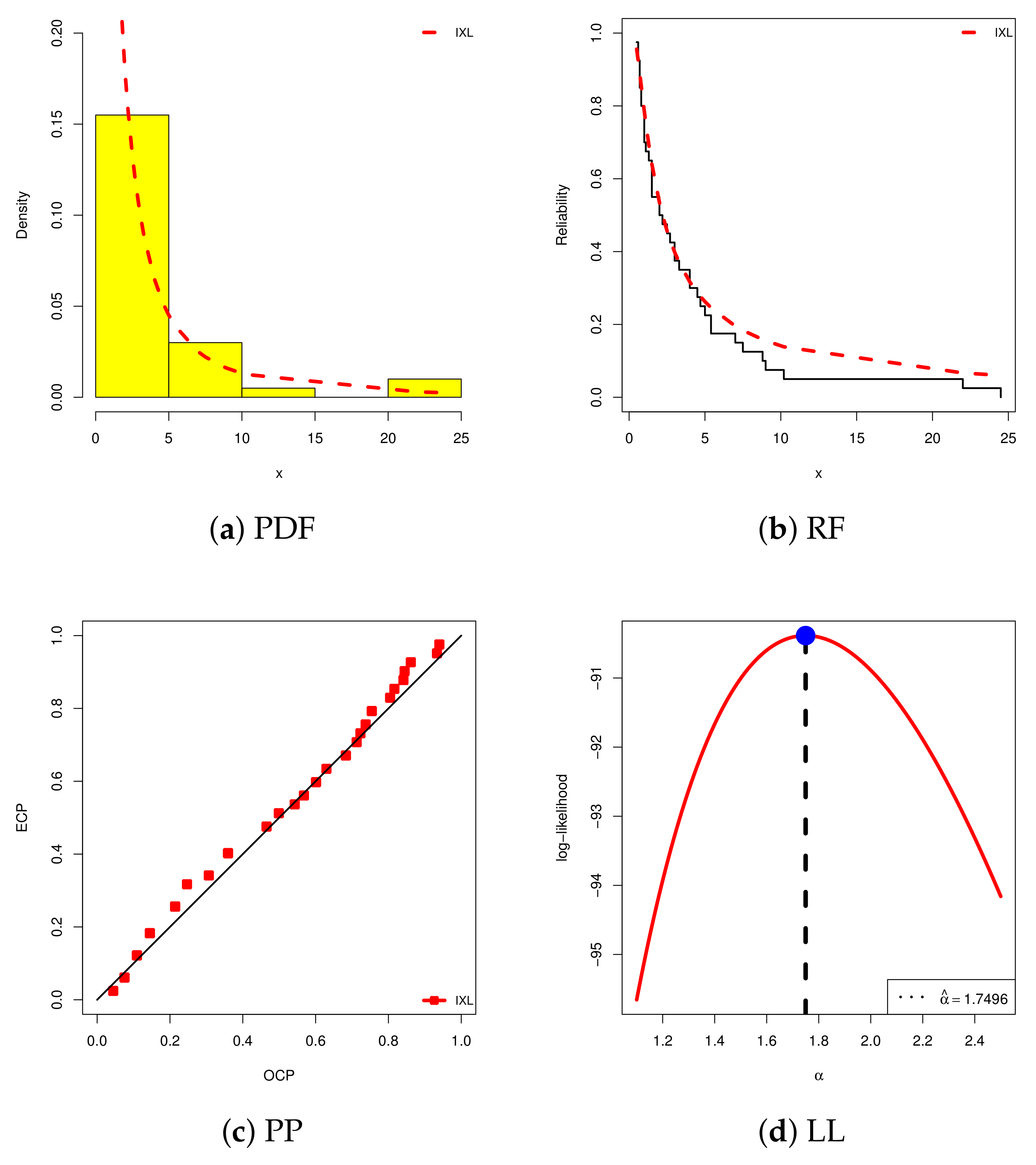
In Figure 5, we employ four visual aids to examine the superiority of the newly formed IXL model, namely (i) the estimated PDF, (ii) the estimated RF, (iii) the estimated probability–probability (PP), and (iv) the log-likelihood (LL). This confirms that the IXL model under investigation is the best option and reflects the computational information provided in Table 16. Additionally, from Figure 5d, the frequentist estimate of $\alpha$ exists and is unique, as well as being chosen as the initial guess in all subsequent evaluations.

From Table 15, based on different levels of $T_i,i=1,2$ and $S_i,i=1,2,...,m,$ three IT2-APC samples (with $m=20$) are obtained; see

Table 17. Three IT2-APC samples from ACT data.

Sample	$({\mathit{S}}_1,{\mathit{S}}_2,\mathit{\dots },{\mathit{S}}_{\mathit{m}})$	${\mathit{T}}_1\left({\mathit{d}}_1\right)$	${\mathit{T}}_2\left({\mathit{d}}_2\right)$	${\mathit{S}}^{*}$	${\mathit{T}}^{*}$	Data
$\mathcal{S}$1	$(5\ast 4,0\ast 16)$	7.75(20)	8.25(20)	0	7.50	0.50, 0.60, 0.70, 0.70, 0.80, 1.00, 1.10, 1.30, 1.50, 2.00,
						2.20, 2.50, 3.00, 3.30, 4.00, 4.50, 4.70, 5.00, 5.40, 7.50
$\mathcal{S}$2	$(0\ast 8,5\ast 4,0\ast 8)$	1.35(11)	4.25(20)	5	4.00	0.50, 0.60, 0.60, 0.70, 0.70, 0.70, 0.80, 0.80, 1.00, 1.00,
						1.30, 1.50, 1.50, 2.00, 2.00, 2.50, 2.70, 3.00, 3.30, 4.00
$\mathcal{S}$3	$(0\ast 16,5\ast 4)$	1.75(17)	2.75(19)	16	2.75	0.50, 0.60, 0.60, 0.70, 0.70, 0.70, 0.80, 0.80, 1.00, 1.00,
						1.00, 1.00, 1.10, 1.30, 1.50, 1.50, 1.50, 2.00, 2.50

. Because prior knowledge on the IXL model from the collection of the ACT data is unavailable, the Bayes estimates, in addition to their BCI/HPD interval estimates of $\alpha$, $R\left(t\right)$, or $h\left(t\right)$ (at $t=1$), are obtained using the gamma improper prior. By simulating 40,000 MCMC iterations and discarding the first of them as 10,000 burn-ins, following the M-H steps, the Bayes point and interval estimates are computed. For each artificial sample and for each unknown quantity, the point estimations (including the maximum likelihood and Bayes MCMC methods) with their St.Errs and the interval estimations (including the 95% ACIs-NA, ACIs-NL, BCIs, and HPD intervals) with their interval lengths (ILs) are obtained; see

Table 18. Estimates of $\alpha$, $R\left(t\right)$, and $h\left(t\right)$ from ACT data.

Sample	Par.	MLE		MCMC		ACI-NA			BCI
						ACI-NL			HPD
		Est.	SE	Est.	SE	Low.	Upp.	IL	Low.	Upp.	IL
$\mathcal{S}1$	$\alpha$	1.8669	0.2911	1.8835	0.2116	1.2964	2.4374	1.1410	1.4865	2.3142	0.8276
						1.3753	2.5342	1.1589	1.4706	2.2970	0.8264
	$R\left(1\right)$	0.8103	0.0569	0.8091	0.0412	0.6988	0.9218	0.2230	0.7195	0.8803	0.1609
						0.7061	0.9298	0.2237	0.7241	0.8834	0.1594
	$h\left(1\right)$	0.3938	0.0759	0.3927	0.0545	0.2450	0.5425	0.2974	0.2909	0.5040	0.2131
						0.2699	0.5745	0.3046	0.2900	0.5026	0.2126
$\mathcal{S}2$	$\alpha$	1.8186	0.2572	1.8328	0.1979	1.3144	2.3227	1.0083	1.4576	2.2341	0.7765
						1.3783	2.3995	1.0213	1.4392	2.2111	0.7719
	$R\left(1\right)$	0.8006	0.0528	0.7995	0.0406	0.6971	0.9041	0.2070	0.7110	0.8700	0.1590
						0.7035	0.9111	0.2076	0.7202	0.8773	0.1572
	$h\left(1\right)$	0.4065	0.0689	0.4056	0.0524	0.2715	0.5416	0.2700	0.3074	0.5134	0.2060
						0.2917	0.5667	0.2750	0.3060	0.5115	0.2055
$\mathcal{S}3$	$\alpha$	1.8210	0.2516	1.8349	0.1954	1.3279	2.3142	0.9863	1.4637	2.2312	0.7675
						1.3890	2.3874	0.9984	1.4518	2.2131	0.7612
	$R\left(1\right)$	0.8011	0.0515	0.8000	0.0400	0.7001	0.9021	0.2020	0.7128	0.8697	0.1568
						0.7062	0.9088	0.2025	0.7208	0.8757	0.1549
	$h\left(1\right)$	0.4059	0.0673	0.4050	0.0517	0.2740	0.5378	0.2638	0.3080	0.5114	0.2033
						0.2933	0.5617	0.2685	0.3055	0.5082	0.2027

. It is clear from Table 18 that the estimates we obtained for $\alpha$, $R\left(t\right)$, or $h\left(t\right)$ using the maximum likelihood and Bayes approaches are very close to each other. The same pattern is also achieved when comparing the calculated asymptotic interval estimates with those created from the credible interval estimates. Moreover, in terms of the minimum St.Err and IL values, the point and interval estimates created using the Bayes MCMC framework behaved better than the others.

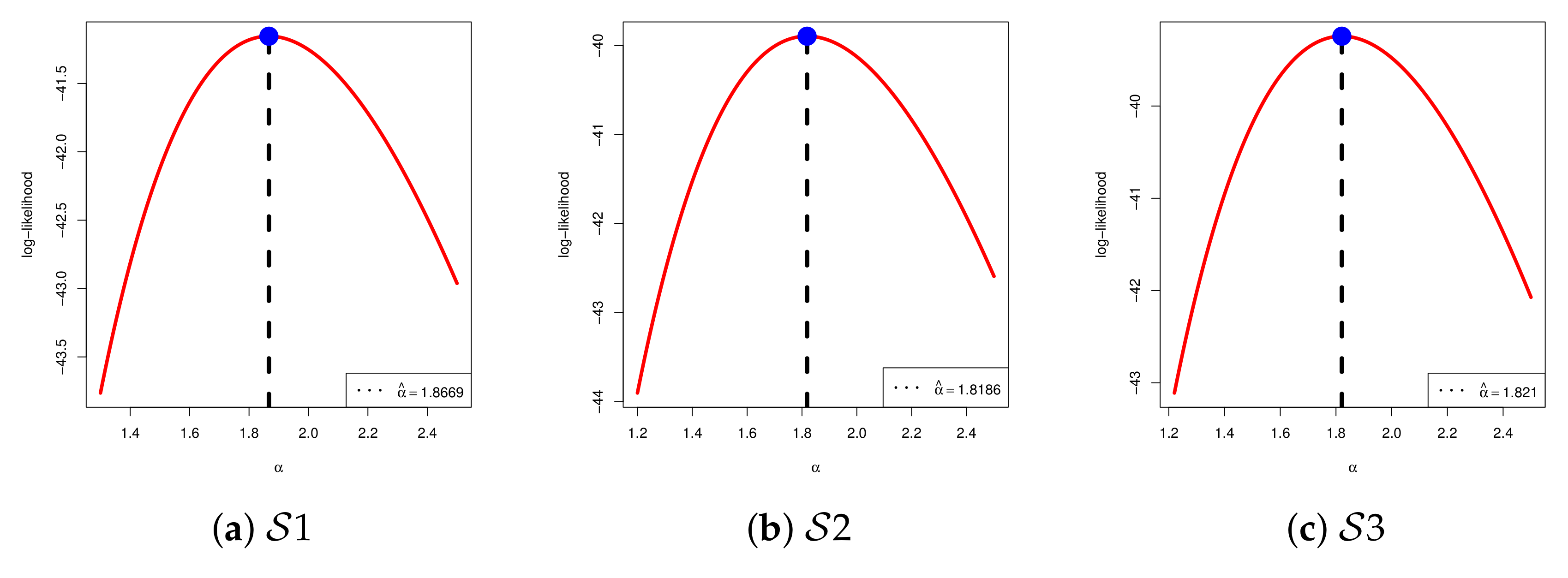
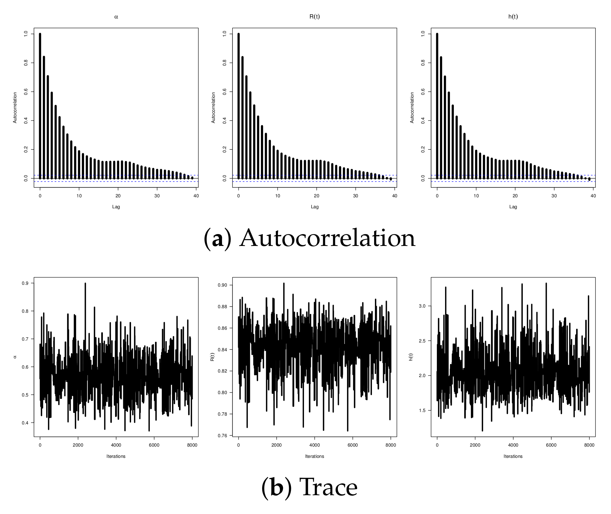
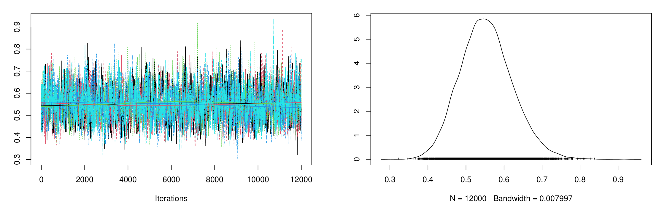
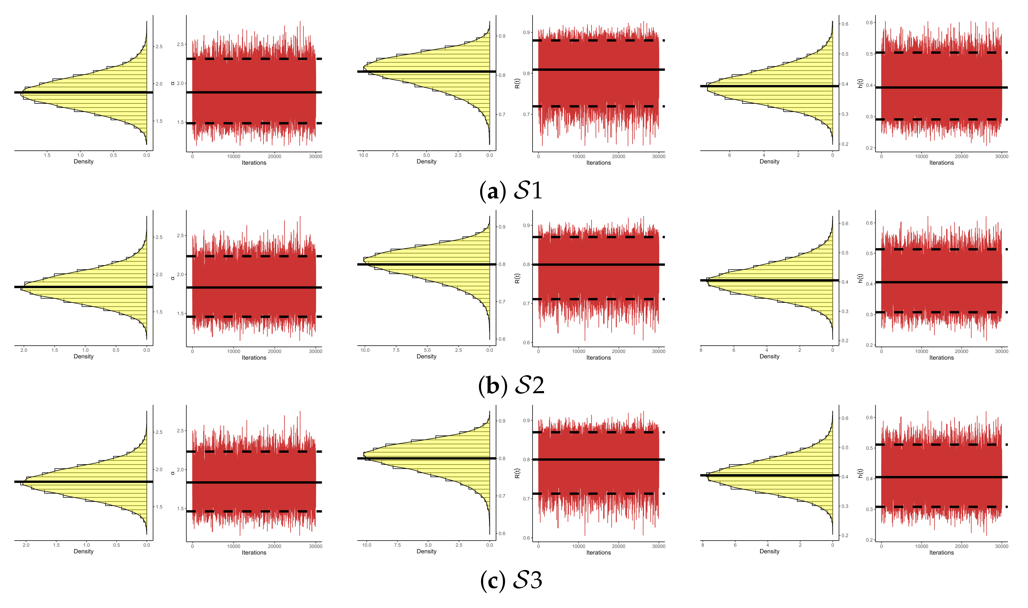
To demonstrate the existence and uniqueness of the MLE of $\alpha$ offered, for $\mathcal{S}i,i=1,2,3,$ the log-likelihood curves shown in Figure 6 illustrate that the MLE of $\alpha$ exists and is unique. On the other hand, to assess the convergence of the 30,000 MCMC iterations of $\alpha$, $R\left(t\right)$, and $h\left(t\right)$ retained, both the trace and trace density for each parameter (using $\mathcal{S}i,i=1,2,3,$) are depicted in Figure 7. To distinguish them, the solid and dashed lines represent the Bayes point and BCI estimates, respectively. It reveals that the MCMC technique converges well, and the recommended burn-in sample size is enough. Furthermore, it also indicates that the 30,000 iterations of $\alpha$ and $h\left(t\right)$ collected are symmetrical, while those of $R\left(t\right)$ are negatively skewed.

To sum up, the ACT system produces bounded or skewed reliability data, making it well suited to the flexible inferential methodologies proposed in our study. Applying the IXL lifespan model within a Bayesian framework enables more accurate modeling of the uncertainty and failure risk, which is critical for reliability and safety assessments in aerospace systems.

6. Concluding Remarks

In this study, point and interval estimates of the scale parameter, the reliability function, and the failure rate function of the inverse XLindley distribution lifetime model are explored under the presence of an improved Type-II adaptive progressive censoring plan. The maximum likelihood method, a conventional approach, is used to estimate the unknown parameters, and two approximate interval estimations are tested using normal approximations of the acquired estimates. Bayesian estimations, on the other hand, incorporate a gamma prior and the squared error loss function. Due to the complex nature of the posterior distribution, Bayes estimates are obtained through sampling using the Metropolis–Hastings algorithm. Additionally, two credible interval estimates are provided. To compare the point estimates obtained using both the classical and Bayesian methodologies, as well as the four interval estimation procedures, a simulation study is carried out using various sampling plans that account for different effective numbers of failures, removal patterns, and threshold times. Based on the findings, we found that the Bayes estimates with informative priors outperform the classical estimates in terms of their minimum root mean square error and mean relative absolute bias. An identical outcome was observed for interval estimations using the interval width and coverage probability criteria. The highest posterior density credible intervals outperformed the Bayes credible intervals, and both were superior to the two classical interval estimates. Finally, the proposed methods were applied to analyzing an actual dataset containing the active repair durations of an airborne communication transceiver. This investigation demonstrated the efficiency of the inverse XLindley distribution across a variety of commonly used models. As a direction for future study, it would be useful to examine Bayesian estimations for the inverse XLindley distribution under asymmetric loss functions, such as the LINEX and general entropy loss functions. These loss functions are mainly suitable for reliability analyses where the costs of overestimation and underestimation may vary. Another possible approach in future research is to explore the estimation challenges for the inverse XLindley distribution in more complex environments, such as scenarios involving numerous reasons for failure, or under accelerated life-testing conditions.