Dynamics of Abundant Wave Solutions to the Fractional Chiral Nonlinear Schrodinger’s Equation: Phase Portraits, Variational Principle and Hamiltonian, Chaotic Behavior, Bifurcation and Sensitivity Analysis

Abstract

The central objective of this study is to develop some different wave solutions and perform a qualitative analysis on the nonlinear dynamics of the time-fractional chiral nonlinear Schrodinger’s equation (NLSE) in the conformable sense. Combined with the semi-inverse method (SIM) and traveling wave transformation, we establish the variational principle (VP). Based on this, the corresponding Hamiltonian is constructed. Adopting the Galilean transformation, the planar dynamical system is derived. Then, the phase portraits are plotted and the bifurcation analysis is presented to expound the existence conditions of the various wave solutions with the different shapes. Furthermore, the chaotic phenomenon is probed and sensitivity analysis is given in detail. Finally, two powerful tools, namely the variational method (VM) which stems from the VP and Ritz method, as well as the Hamiltonian-based method (HBM) that is based on the energy conservation theory, are adopted to find the abundant wave solutions, which are the bell-shape soliton (bright soliton), W-shape soliton (double-bright solitons or double bell-shaped soliton) and periodic wave solutions. The shapes of the attained new diverse wave solutions are simulated graphically, and the impact of the fractional order $\delta$ on the behaviors of the extracted wave solutions are also elaborated. To the authors’ knowledge, the findings of this research have not been reported elsewhere and can enable us to gain a profound understanding of the dynamics characteristics of the investigative equation.

1. Introduction

In the field of nonlinear science, nonlinear partial differential equations (NPDEs) are widely used to describe complex and diverse nonlinear phenomena in nature [1,2,3,4,5,6]. Their exact and approximate solutions play a very important role. Solving NPDEs is the core content of studying nonlinear fields [7,8,9,10]. Due to the complexity of nonlinearity, there is no unified method for finding the exact and approximate solutions. Common approaches for solving NPDEs include the Hirota bilinear approach [11,12,13], Kudryashov’s approach [14,15], Darboux transformation technique [16,17], Sardar subequation technique [18,19], exp-function approach [20,21], Bäcklund transformations [22,23], generalized (G’/G)-expansion method [24,25], generalized auxiliary equation [26,27], trial equation technique [28,29], inverse scattering transformation technique [30,31] and so on. In this article, we first study the chiral NLSE as [32]:

$$i{\psi }_t+\alpha \left({\psi }_{xx}+{\psi }_{yy}\right)+i\left\{{\beta }_1\left(\psi {\psi }_x^{*}-{\psi }^{*}{\psi }_x\right)+{\beta }_2\left(\psi {\psi }_y^{*}-{\psi }^{*}{\psi }_y\right)\right\}\psi =0,$$

(1)

where $\psi =\psi \left(x,y,t\right)$ is a complex function of the space $x$,  $y$ and time $t$ Equation (1) can be used to describe the wave in the quantum field theory, ${\psi }^{\ast }={\psi }^{\ast }\left(x,y,t\right)$ denotes its conjugate form, $\alpha$ is the coefficient of the dispersion term and ${\beta }_1$ and ${\beta }_2$ represent the coefficients of nonlinear coupling terms. In [32], the trial solution technique was used to explore Equation (1). In [33], the modified Jacobi elliptic expansion method was adopted to find the different soliton solutions. In [34], the sine-Gordon expansion approach was employed to obtain the dark and bright wave solutions. In [35], the Fan subequation technique was utilized to find the rich soliton solutions. In [36], the extended rational sine–cosine/sinh–cosh approaches were used and diverse traveling wave solutions were extracted. In [37], the generalized auxiliary equation method was considered to retrieve different soliton solutions. In [38], the extended direct algebraic was used to look into the dark and singular solitons.

Recently, fractional order NPDEs have become popular research topics, since they can better characterize viscoelastic, anomalous diffusion and memory phenomena in nature. Many different fractional derivatives, such as the Atangana–Baleanu fractional derivative [39,40], beta fractional derivative [41,42], Riemann–Liouville fractional derivative [43,44], Caputo fractional derivatives [45,46], conformable fractional derivative [47,48] and others [49,50,51], have been put forward to explore natural phenomena. These different fractional derivatives each have their own characteristics, and some specific comparisons of the conformable fractional derivative and the Riemann–Liouville and Caputo fractional derivatives can be found in [52]. Hereby, in this work, we propose the time-fractional chiral NLSE in the conformable sense as:

$$i{D}_t^{\delta }\psi +\alpha \left({\psi }_{xx}+{\psi }_{yy}\right)+i\left\{{\beta }_1\left(\psi {\psi }_x^{*}-{\psi }^{*}{\psi }_x\right)+{\beta }_2\left(\psi {\psi }_y^{*}-{\psi }^{*}{\psi }_y\right)\right\}\psi =0,$$

(2)

where $D_t^{\delta }$ is the conformable fractional partial derivative regarding the time $t$ with the fractional order $\delta$ for a function $\psi$: $R\times \left(0,\infty \right)\to R$ as [53]:

$$D_t^{\delta }\psi \left(x,y,t\right)=\underset{\epsilon \to 0}{\lim }{\displaystyle \frac{\psi \left(x,y,t+\epsilon t^{1-\delta }\right)-\psi \left(x,y,t\right)}{\epsilon }}.$$

(3)

for all $t>0$, $\delta \in \left[0,1\right)$. There are the following properties [53]:

$$D_t^{\delta }\left(a\psi +b\phi \right)=a{D}_t^{\delta }\psi +b{D}_t^{\delta }\phi ,$$

(4)

$$D_t^{\delta }\left(t^p\right)=p{t}^{p-\delta }, \forall p\in R,$$

(5)

$$D_t^{\delta }\left(\lambda \right)=0,$$

(6)

where $\lambda$ is a constant.

$$D_t^{\delta }\left(\psi \phi \right)=\phi D_t^{\delta }\psi +\psi D_t^{\delta }\phi ,$$

(7)

$$D_t^{\delta }\left(\psi /\phi \right)={\displaystyle \frac{\phi D_t^{\delta }\psi -\psi D_t^{\delta }\phi }{{\phi }^2}},$$

(8)

If $\psi$ is differentiable with respect to $t$, then:

$$D_t^{\delta }\psi \left(x,y,t\right)=t^{1-\delta }{\displaystyle \frac{\partial \psi \left(x,y,t\right)}{t}}.$$

(9)

where $\psi =\psi \left(x,y,t\right)$ and $\phi =\phi \left(x,y,t\right)$.

We can see that Equation (2) simplifies to the classic chiral NLSE in Equation (1) for $\delta =1$ In this work, we will give a qualitative analysis of Equation (1) through the theory of the planar dynamical system and develop diverse wave solutions through two analytic methods, namely the VM and HBM, which are different from the symbol calculation method methods used in [32,33,34,35,36,37,38]. The VM and HBM are more simple and straightforward and do not involve symbol calculation, which can avoid a lot of redundant calculations. The remaining content of this article is arranged as follows. The VP and the Hamiltonian function are explored in Section 2. In Section 3, a quantitative analysis of the system is presented. In Section 4, the VM and HBM are used to develop diverse wave solutions. In Section 5, the results and discussion are presented. Finally, a summary is given in Section 6.

2. The Variational Principle and Hamiltonian

The task of the current section is to create the VP with the aid of the SIM and extract the Hamiltonian of the system. To this end, we manipulate the following transformation:

$$\psi \left(x,y,t\right)=\Xi \left(\varsigma \right)e^{i\eta }, \varsigma ={\epsilon }_{1}x+{\mu }_{1}y+\frac{{\kappa }_1}{\delta }{t}^{\delta }+{\varsigma }_0, \eta ={\epsilon }_{2}x+{\mu }_{2}y+\frac{{\kappa }_2}{\delta }{t}^{\delta }+{\eta }_0,$$

(10)

where ${\epsilon }_i$ (i = 1, 2), ${\mu }_i$ (i = 1, 2) and ${\kappa }_i$ (i = 1, 2) are non-zero real constants, and ${\varsigma }_0$ and ${\eta }_0$ are real constants. By substituting them into Equation (2) and applying the properties of the conformable fractional partial derivative, we obtain:

$$i{D}_t^{\delta }\psi =\left(i{k}_1{\displaystyle \frac{d\Xi }{d\varsigma }}-k_2\Xi \right)e^{i\eta },$$

(11)

$${\psi }_{xx}=\left({\epsilon }_1^2{\displaystyle \frac{d^2\Xi }{d{\varsigma }^2}}+2i{\epsilon }_1{\epsilon }_2{\displaystyle \frac{d\Xi }{d\varsigma }}-{\epsilon }_2^2\Xi \right)e^{i\eta },$$

(12)

$${\psi }_{yy}=\left({\mu }_1^2{\displaystyle \frac{d^2\Xi }{d{\varsigma }^2}}+2i{\mu }_1{\mu }_2{\displaystyle \frac{d\Xi }{d\varsigma }}-{\mu }_2^2\Xi \right)e^{i\eta },$$

(13)

$$\left(\psi {\psi }_x^{*}-{\psi }^{*}{\psi }_x\right)\psi =-2i{\epsilon }_2{\Xi }^3{e}^{i\eta },$$

(14)

and

$$\left(\psi {\psi }_y^{*}-{\psi }^{*}{\psi }_y\right)\psi =-2i{\mu }_2{\Xi }^3{e}^{i\eta }.$$

(15)

Taking them into Equation (2) yields:

$$\begin{array}{l}i{\kappa }_1{\Xi }^{\prime }\left(\varsigma \right)-{\kappa }_2\Xi \left(\varsigma \right)+\alpha \lfloor \left({\epsilon }_1^2+{\mu }_1^2\right){\Xi }^{″}\left(\varsigma \right)+2i\left({\epsilon }_1{\epsilon }_2+{\mu }_1{\mu }_2\right){\Xi }^{\prime }\left(\varsigma \right)-\left({\epsilon }_2^2+{\mu }_2^2\right)\Xi \left(\varsigma \right)\rfloor \\ -i\left(2i{\beta }_1{\epsilon }_2+2i{\beta }_2{\mu }_2\right){\Xi }^3\left(\varsigma \right)=0\end{array},$$

(16)

Its real and imaginary parts are obtained, respectively, as:

$$\alpha \left({\epsilon }_1^2+{\mu }_1^2\right){\Xi }^{″}\left(\varsigma \right)-\lfloor \alpha \left({\epsilon }_2^2+{\mu }_2^2\right)+{\kappa }_2\rfloor \Xi \left(\varsigma \right)+2\left({\beta }_1{\epsilon }_2+{\beta }_2{\mu }_2\right){\Xi }^3\left(\varsigma \right)=0.$$

(17)

and

$${\Xi }^{\prime }\left(\varsigma \right)\left[2\alpha \left({\epsilon }_1{\epsilon }_2+{\mu }_1{\mu }_2\right)+{\kappa }_1\right]=0.$$

(18)

By Equation (18), we obtain:

$${\kappa }_1=-2\alpha \left({\epsilon }_1{\epsilon }_2+{\mu }_1{\mu }_2\right).$$

(19)

Equation (17) can be re-written as:

$${\Xi }^{″}\left(\varsigma \right)-{\displaystyle \frac{\alpha \left({\epsilon }_2^2+{\mu }_2^2\right)+{\kappa }_2}{\alpha \left({\epsilon }_1^2+{\mu }_1^2\right)}}\Xi \left(\varsigma \right)+{\displaystyle \frac{2\left({\beta }_1{\epsilon }_2+{\beta }_2{\mu }_2\right)}{\alpha \left({\epsilon }_1^2+{\mu }_1^2\right)}}{\Xi }^3\left(\varsigma \right)=0.$$

(20)

where $\alpha \left({\epsilon }_2^2+{\mu }_2^2\right)+{\kappa }_2\ne 0$ and ${\beta }_1{\epsilon }_2+{\beta }_2{\mu }_2\ne 0$. We can establish its VP by employing the SIM as [54,55,56,57]:

$$J\left(\Xi \right)={\displaystyle {\int }_0^{\infty }\left\{\frac{1}{2}{\left({\Xi }^{\prime }\right)}^2+\frac{\alpha \left({\epsilon }_2^2+{\mu }_2^2\right)+{\kappa }_2}{2\alpha \left({\epsilon }_1^2+{\mu }_1^2\right)}{\Xi }^2-\frac{\left({\beta }_1{\epsilon }_2+{\beta }_2{\mu }_2\right)}{2\alpha \left({\epsilon }_1^2+{\mu }_1^2\right)}{\Xi }^4\right\}}d\varsigma ,$$

(21)

which can be expressed as [58]:

$$\begin{array}{ll}J\left(\Xi \right)& ={\displaystyle {\int }_0^{\infty }\left\{\frac{1}{2}{\left({\Xi }^{\prime }\right)}^2+\frac{\alpha \left({\epsilon }_2^2+{\mu }_2^2\right)+{\kappa }_2}{2\alpha \left({\epsilon }_1^2+{\mu }_1^2\right)}{\Xi }^2-\frac{\left({\beta }_1{\epsilon }_2+{\beta }_2{\mu }_2\right)}{2\alpha \left({\epsilon }_1^2+{\mu }_1^2\right)}{\Xi }^4\right\}}d\varsigma \\ & ={\displaystyle {\int }_0^{\infty }\left\{K-P\right\}}d\varsigma \end{array}.$$

(22)

where $K$ and $P$ stand for the kinetic energy and potential energy of the system, respectively, as follows:

$$K={\displaystyle \frac{1}{2}}{\left({\Xi }^{\prime }\right)}^2,$$

(23)

$$P=-{\displaystyle \frac{\alpha \left({\epsilon }_2^2+{\mu }_2^2\right)+{\kappa }_2}{2\alpha \left({\epsilon }_1^2+{\mu }_1^2\right)}}{\Xi }^2+{\displaystyle \frac{\left({\beta }_1{\epsilon }_2+{\beta }_2{\mu }_2\right)}{2\alpha \left({\epsilon }_1^2+{\mu }_1^2\right)}}{\Xi }^4.$$

(24)

Then, we can get the Hamiltonian of the system as follows:

$$H=K+P={\displaystyle \frac{1}{2}}{\left({\Xi }^{\prime }\right)}^2-{\displaystyle \frac{\alpha \left({\epsilon }_2^2+{\mu }_2^2\right)+{\kappa }_2}{2\alpha \left({\epsilon }_1^2+{\mu }_1^2\right)}}{\Xi }^2+{\displaystyle \frac{\left({\beta }_1{\epsilon }_2+{\beta }_2{\mu }_2\right)}{2\alpha \left({\epsilon }_1^2+{\mu }_1^2\right)}}{\Xi }^4.$$

(25)

3. The Bifurcation, Chaotic and Sensitivity Analysis, and the Existence Condition of the Various Wave Solutions

3.1. Bifurcation Analysis

Adopting the Galilean transformation to Equation (20), we can achieve the following dynamical system [59]:

$$\left\{\begin{array}{l}{\displaystyle \frac{d\Xi }{d\varsigma }}=\varphi \\ {\displaystyle \frac{d\varphi }{d\varsigma }}=s_1\Xi \left(\varsigma \right)-s_2{\Xi }^3\left(\varsigma \right)\end{array}\right.,$$

(26)

with

$$s_1={\displaystyle \frac{\alpha \left({\epsilon }_2^2+{\mu }_2^2\right)+{\kappa }_2}{\alpha \left({\epsilon }_1^2+{\mu }_1^2\right)}}, s_2=\frac{2\left({\beta }_1{\epsilon }_2+{\beta }_2{\mu }_2\right)}{\alpha \left({\epsilon }_1^2+{\mu }_1^2\right)}.$$

(27)

The equilibrium points of system Equation (26) can be found via setting:

$$\left\{\begin{array}{l}\varphi =0\\ s_1\Xi -s_2{\Xi }^3=0\end{array}\right..$$

(28)

Then, we can get the equilibrium points as:

$$e_0=\left(0,0\right), e_1=\left(-\sqrt{\frac{s_1}{s_2}},0\right), e_2=\left(\sqrt{\frac{s_1}{s_2}},0\right).$$

(29)

Based on Equation (26), we have:

$$f^{\prime }\left(\Xi \right)=s_1-3s_2{\Xi }^2.$$

(30)

Therefore, the Jacobi matrix at the $e_i\left(i=0,1,2\right)$ is:

$$J\left(e_i,0\right)=\left(\begin{array}{cc}0& 1\\ s_1-3s_2{\Xi }^2& 0\end{array}\right).$$

(31)

And its determinant can be written as:

$$Det\left(J\left(e_i,0\right)\right)=\left|\begin{array}{cc}0& 1\\ s_1-3s_2{\Xi }^2& 0\end{array}\right|=-s_1+3s_2{\Xi }^2.$$

(32)

Therefore, we know the following:

I: When $J\left(e_i,0\right)>0$, the corresponding point $e_i$ is the center point.

II: When $J\left(e_i,0\right)<0$, the corresponding point $e_i$ is the saddle point.

III: When $J\left(e_i,0\right)=0$, the corresponding point $e_i$ is the cuspidal point.

Further:

Case 1: When $s_1>0$ and $s_2>0$, $J\left(0,0\right)=-s_1<0$, $e_0$ is the saddle point. $J\left(-\sqrt{{\displaystyle \frac{s_1}{s_2}}},0\right)=2s_1>0$ and $J\left(\sqrt{{\displaystyle \frac{s_1}{s_2}}},0\right)=2s_1>0$, thus $e_1$ and $e_2$ are the center points. If the parameters are used as $\alpha =1$, ${\beta }_1=1$, ${\beta }_2=1$, ${\epsilon }_1=1$, ${\epsilon }_2=1$, ${\mu }_1=1$, ${\mu }_2=1$ and ${\kappa }_2=1$, we find three points $\left(0,0\right)$, $\left(-{\displaystyle \frac{\sqrt{3}}{2}},0\right)$ and $\left({\displaystyle \frac{\sqrt{3}}{2}},0\right)$. Here, we can see from Figure 1a that the point $\left(0,0\right)$ is the saddle point, and $\left(-{\displaystyle \frac{\sqrt{3}}{2}},0\right)$ and $\left({\displaystyle \frac{\sqrt{3}}{2}},0\right)$ are the center points.

Case 2: When $s_1>0$ and $s_2<0$, there is only one equilibrium point $e_0$, and $J\left(0,0\right)=-s_1<0$, thus $e_0$ is the saddle point. For $\alpha =1$, ${\beta }_1=-1$, ${\beta }_2=-1$, ${\epsilon }_1=1$, ${\epsilon }_2=1$,  ${\mu }_1=1$, ${\mu }_2=1$ and ${\kappa }_2=1$, we have only one equilibrium point as $\left(0,0\right)$ that is shown in Figure 1b, where it can be seen that the $\left(0,0\right)$ is the saddle point.

Case 3: When $s_1<0$ and $s_2<0$, $J\left(0,0\right)=-s_1>0$, $e_0$ is the center point. $J\left(-\sqrt{{\displaystyle \frac{s_1}{s_2}}},0\right)=2s_1<0$ and $J\left(\sqrt{{\displaystyle \frac{s_1}{s_2}}},0\right)=2s_1<0$, thus $e_1$ and $e_2$ are the saddle points. In this case, when the parameter values are chosen as $\alpha =-1$, ${\beta }_1=1$, ${\beta }_2=1$, ${\epsilon }_1=1$, ${\epsilon }_2=1$, ${\mu }_1=1$, ${\mu }_2=1$ and ${\kappa }_2=5$, Figure 1c plots the two equilibrium points as $\left(0,0\right)$ and $\left(-1,0\right)$, where we find that the point $\left(0,0\right)$ is the center point and $\left(-1,0\right)$ is a saddle point.

Case 4: When $s_1<0$ and $s_2>0$, there is only one equilibrium point $e_0$, and $J\left(0,0\right)=-s_1>0$, thus $e_0$ is the center point. If the parameter values are used as $\alpha =-1$, ${\beta }_1=-1$, ${\beta }_2=-1$, ${\epsilon }_1=1$, ${\epsilon }_2=1$, ${\mu }_1=1$, ${\mu }_2=1$ and ${\kappa }_2=5$, the only equilibrium point $e_0\left(0,0\right)$ is presented in Figure 1d. Obviously, the point $\left(0,0\right)$ is the center point.

3.2. The Existence Conditions of the Various Wave Solutions

By the theory of planar dynamical systems, we know that the bell-shaped soliton solution, periodic solution, kink soliton solution and unbounded traveling wave solution correspond to the homoclinic orbit, closed orbit, heteroclinic orbit and opened orbit, respectively. Thus, we can conclude that

(1)

When $s_1>0$ and $s_2>0$, Equation (20) has the bell-shaped soliton and periodic wave solutions (see Figure 1a).

(2)

When $s_1>0$ and $s_2<0$, Equation (20) has unbounded traveling wave solutions (see Figure 1b).

(3)

When $s_1<0$ and $s_2>0$, Equation (20) has the kink soliton and periodic wave solutions (see Figure 1c).

(4)

When $s_1<0$ and $s_2<0$, Equation (20) has the periodic wave solutions (see Figure 1d).

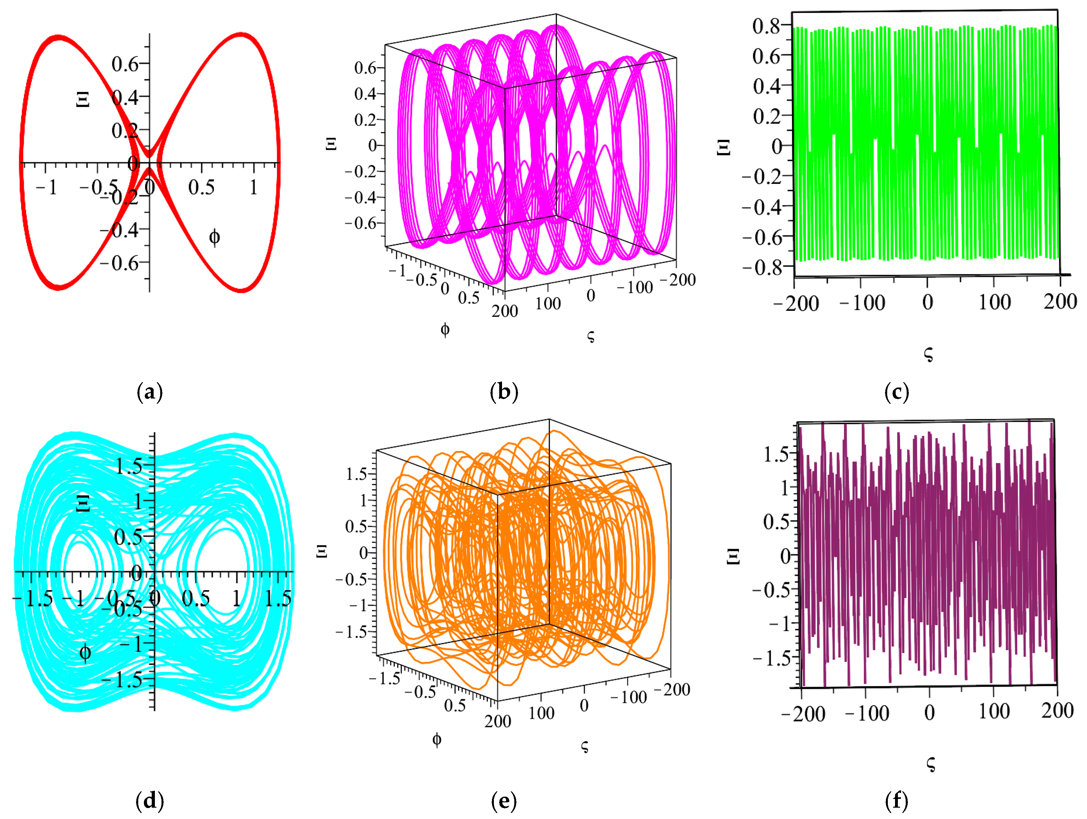
3.3. The Quasi-Periodic and Chaotic Behaviors

This part aims to explore the quasi-periodic and chaotic behaviors of the system by adding a perturbed term. For this purpose, here we can take the trigonometric function as the external perturbed term [60,61]:

$$\left\{\begin{array}{l}{\displaystyle \frac{d\Xi }{d\varsigma }}=\varphi \\ {\displaystyle \frac{d\varphi }{d\varsigma }}=s_1\Xi \left(\varsigma \right)-s_2{\Xi }^3\left(\varsigma \right)+\Lambda \cos (\varpi \varsigma )\end{array}\right..$$

(33)

where $\Lambda$ represents the amplitude and $\varpi$ stands for the frequency. Obviously, the parameters $s_1$, $s_2$, $\Lambda$ and $\varpi$ may affect the periodic and chaotic dynamical behaviors. To elaborate the corresponding phenomenon, here the parameters are chosen as $\alpha =1$, ${\beta }_1=1$, ${\beta }_2=1$, ${\epsilon }_1=1$, ${\epsilon }_2=1$, ${\mu }_1=1$, ${\mu }_2=1$ and ${\kappa }_2=1$, and then the 2- and 3D phase portraits and the time series plot for the different $\Lambda$ and $k$ with the initial conditions as $\Xi \left(0\right)=0.1$ and $\varphi \left(0\right)=0$ are presented in Figure 2, where (a–c) for $\Lambda =0.04$, $\varpi =0.1$, and (d–f) for $\Lambda =0.5$, $\varpi =0.8$. We find the system is quasi-periodic at $\Lambda =0.04$, $\psi =0.1$, but it becomes chaotic when $\Lambda =0.5$, $\varpi =0.8$.

3.4. The Sensitivity Analysis

In this subsection, we will explore the planar dynamical system’s sensitivity characteristics through He’s frequency–amplitude formulation method for $\alpha =-1$, ${\beta }_1=-1$,  ${\beta }_2=-1$,  ${\epsilon }_1=1$, ${\epsilon }_2=1$, ${\mu }_1=1$, ${\mu }_2=1$ and ${\kappa }_2=5$ with the initial conditions as (a) $\Xi \left(0\right)=0.5$, $\varphi \left(0\right)=0.1$, (b) $\Xi \left(0\right)=0.4$, $\varphi \left(0\right)=0.2$ and (c) $\Xi \left(0\right)=0.5$, $\varphi \left(0\right)=0.2$. From the compared results in Figure 3, we can see that small changes in the initial conditions can affect the behaviors of the solution greatly.

4. The Abundant Wave Solutions

In this part, we aim to develop the abundant wave solutions by the VM and the HBM.

4.1. The Variational Method

Family one

According to VM, it is assumed that the solution of Equation (20) is [62]:

$$\Xi =\Theta \sec \mathrm{h}\left(\varsigma \right),$$

(34)

Now we can re-write Equation (21) as:

$$J\left(\Xi \right)={\displaystyle {\int }_0^{\infty }\left\{\frac{1}{2}{\left({\Xi }^{\prime }\right)}^2+{\Im }_1{\Xi }^2-{\Im }_2{\Xi }^4\right\}}d\varsigma .$$

(35)

where ${\Im }_1={\displaystyle \frac{\alpha \left({\epsilon }_2^2+{\mu }_2^2\right)+{\kappa }_2}{2\alpha \left({\epsilon }_1^2+{\mu }_1^2\right)}}$, ${\Im }_2={\displaystyle \frac{\left({\beta }_1{\epsilon }_2+{\beta }_2{\mu }_2\right)}{2\alpha \left({\epsilon }_1^2+{\mu }_1^2\right)}}$.

Taking Equation (34) into Equation (35) yields:

$$\begin{array}{ll}J\left(\Theta \right)& ={\displaystyle {\int }_0^{\infty }\left\{\frac{1}{2}{\left({\Xi }^{\prime }\right)}^2+{\Im }_1{\Xi }^2-{\Im }_2{\Xi }^4\right\}}d\varsigma \\ & ={\displaystyle {\int }_0^{\infty }\left\{\frac{1}{2}{\left[-\Theta \sec \mathrm{h}\left(\varsigma \right)\tan \mathrm{h}\left(\varsigma \right)\right]}^2-{\Im }_1{\left[\Theta \sec \mathrm{h}\left(\varsigma \right)\right]}^2-{\Im }_2{\left[\Theta \sec \mathrm{h}\left(\varsigma \right)\right]}^4\right\}}d\varsigma \\ & ={\displaystyle \frac{{\Theta }^2}{6}}\left(1+6{\Im }_1-4{\Theta }^2{\Im }_2\right)\end{array}.$$

(36)

Computing its stationary condition by the Ritz method as

$${\displaystyle \frac{dJ\left(\Theta \right)}{d\Theta }}=0,$$

(37)

which leads to:

$${\displaystyle \frac{1}{3}}\left(\Theta +6\Theta {\Im }_1-8{\Theta }^3{\Im }_2\right)=0.$$

(38)

By solving it, we obtain:

$$\Theta =\pm {\displaystyle \frac{1}{2}}\sqrt{{\displaystyle \frac{6{\Im }_1+1}{2{\Im }_2}}}.$$

(39)

which is:

$$\Theta =\pm {\displaystyle \frac{1}{2}}\sqrt{{\displaystyle \frac{3\alpha \left({\epsilon }_2^2+{\mu }_2^2\right)+3{\kappa }_2+\alpha \left({\epsilon }_1^2+{\mu }_1^2\right)}{{\beta }_1{\epsilon }_2+{\beta }_2{\mu }_2}}}.$$

(40)

Thus, we have:

$$\Xi =\pm {\displaystyle \frac{1}{2}}\sqrt{{\displaystyle \frac{3\alpha \left({\epsilon }_2^2+{\mu }_2^2\right)+3{\kappa }_2+\alpha \left({\epsilon }_1^2+{\mu }_1^2\right)}{{\beta }_1{\epsilon }_2+{\beta }_2{\mu }_2}}}\sec \mathrm{h}\left(\varsigma \right).$$

(41)

Thus, the bell-shape soliton solution is obtained as:

$${\psi }^{\pm }\left(x,y,t\right)=\pm \frac{1}{2}\sqrt{\frac{3\alpha \left({\epsilon }_2^2+{\mu }_2^2\right)+3{\kappa }_2+\alpha \left({\epsilon }_1^2+{\mu }_1^2\right)}{{\beta }_1{\epsilon }_2+{\beta }_2{\mu }_2}}\text{sech}\left[\begin{array}{l}{\epsilon }_{1}x+{\mu }_{1}y\\ -\frac{2\alpha \left({\epsilon }_1{\epsilon }_2+{\mu }_1{\mu }_2\right)}{\delta }{t}^{\delta }+{\varsigma }_0\end{array}\right]e^{i\left({\epsilon }_{2}x+{\mu }_{2}y+\frac{{\kappa }_2}{\delta }{t}^{\delta }+{\eta }_0\right)}.$$

(42)

which can correspond to the discussion on the existence conditions of the various wave solutions with the different shapes in Section 3.2.

Family two

The solution of Equation (20) can be set as [62]:

$$\Xi =\frac{\Theta \text{sinh}\left(\varsigma \right)}{{\left[\cosh \left(\varsigma \right)\right]}^{\frac{3}{2}}}$$

(43)

Putting it into Equation (35) yields:

$$\begin{array}{ll}J\left(\Theta \right)& ={\displaystyle {\int }_0^{\infty }\left\{\frac{1}{2}{\left({\Xi }^{\prime }\right)}^2+{\Im }_1{\Xi }^2-{\Im }_2{\Xi }^4\right\}}d\varsigma \\ & ={\displaystyle {\int }_0^{\infty }\left\{\frac{1}{2}{\left[\frac{\Theta }{{\left[\cosh \left(\varsigma \right)\right]}^{\frac{1}{2}}}-\frac{3\Theta {\sin \mathrm{h}}^2\left(\varsigma \right)}{2{\left[\cosh \left(\varsigma \right)\right]}^{\frac{5}{2}}}\right]}^2+{\Im }_1{\left[\frac{\Theta \sin \mathrm{h}\left(\varsigma \right)}{{\left[\cosh \left(\varsigma \right)\right]}^{\frac{3}{2}}}\right]}^2-{\Im }_2{\left[\frac{\Theta \sin \mathrm{h}\left(\varsigma \right)}{{\left[\cosh \left(\varsigma \right)\right]}^{\frac{3}{2}}}\right]}^4\right\}}d\varsigma \\ & ={\displaystyle \frac{{\Theta }^2}{640}}\left[5\pi \left(11+32{\Im }_1\right)-128{\Theta }^2{\Im }_2\right]\end{array}.$$

(44)

Taking its stationary condition as:

$${\displaystyle \frac{dJ\left(\Theta \right)}{d\Theta }}=0,$$

(45)

which leads to:

$${\displaystyle \frac{1}{64}}\Theta \pi \left(11+32{\Im }_1\right)-{\displaystyle \frac{4{\Theta }^3{\Im }_2}{5}}=0.$$

(46)

Solving it gives:

$$\Theta =\pm {\displaystyle \frac{1}{16}}\sqrt{{\displaystyle \frac{5\pi \left(11+32{\Im }_1\right)}{{\Im }_2}}},$$

(47)

which is:

$$\Theta =\pm {\displaystyle \frac{1}{16}}\sqrt{{\displaystyle \frac{110\pi \alpha \left({\epsilon }_1^2+{\mu }_1^2\right)+160\pi \left[\alpha \left({\epsilon }_2^2+{\mu }_2^2\right)+{\kappa }_2\right]}{{\beta }_1{\epsilon }_2+{\beta }_2{\mu }_2}}}.$$

(48)

Then, we have:

$$\Xi =\pm {\displaystyle \frac{1}{16}}\sqrt{{\displaystyle \frac{110\pi \alpha \left({\epsilon }_1^2+{\mu }_1^2\right)+160\pi \left[\alpha \left({\epsilon }_2^2+{\mu }_2^2\right)+{\kappa }_2\right]}{{\beta }_1{\epsilon }_2+{\beta }_2{\mu }_2}}}{\displaystyle \frac{\sin \mathrm{h}\left(\varsigma \right)}{{\left[\cosh \left(\varsigma \right)\right]}^{\frac{3}{2}}}}.$$

(49)

Then, there is:

$$\psi \left(x,y,t\right)=\pm {\displaystyle \frac{1}{16}}\sqrt{{\displaystyle \frac{110\pi \alpha \left({\epsilon }_1^2+{\mu }_1^2\right)+160\pi \left[\alpha \left({\epsilon }_2^2+{\mu }_2^2\right)+{\kappa }_2\right]}{{\beta }_1{\epsilon }_2+{\beta }_2{\mu }_2}}}{\displaystyle \frac{\sin \mathrm{h}\left[\begin{array}{l}{\epsilon }_{1}x+{\mu }_{1}y\\ -\frac{2\alpha \left({\epsilon }_1{\epsilon }_2+{\mu }_1{\mu }_2\right)}{\delta }{t}^{\delta }+{\varsigma }_0\end{array}\right]}{{\left[\cosh \left(\begin{array}{l}{\epsilon }_{1}x+{\mu }_{1}y\\ -\frac{2\alpha \left({\epsilon }_1{\epsilon }_2+{\mu }_1{\mu }_2\right)}{\delta }{t}^{\delta }+{\varsigma }_0\end{array}\right)\right]}^{\frac{3}{2}}}}{e}^{i\left({\epsilon }_{2}x+{\mu }_{2}y+{\displaystyle \frac{{\kappa }_2}{\delta }}{t}^{\delta }+{\eta }_0\right)}.$$

(50)

Family three

Here, we can set [62]:

$$\Xi \left(\varsigma \right)={\displaystyle \frac{\Theta }{1+\cosh \left(\varsigma \right)}}.$$

(51)

Putting Equation (51) into Equation (35) yields:

$$\begin{array}{ll}J\left(\Theta \right)& ={\displaystyle {\int }_0^{\infty }\left\{\frac{1}{2}{\left({\Xi }^{\prime }\right)}^2+{\Im }_1{\Xi }^2-{\Im }_2{\Xi }^4\right\}}d\varsigma \\ & ={\displaystyle {\int }_0^{\infty }\left\{\frac{1}{2}{\left[-\frac{\Theta \sin \mathrm{h}\left(\varsigma \right)}{{\left[1+\cosh \left(\varsigma \right)\right]}^2}\right]}^2+{\Im }_1{\left[\frac{\Theta }{1+\cosh \left(\varsigma \right)}\right]}^2-{\Im }_2{\left[\frac{\Theta }{1+\cosh \left(\varsigma \right)}\right]}^3\right\}}d\varsigma \\ & ={\displaystyle \frac{{\Theta }^2}{210}}\left(7+70{\Im }_1-12{\Theta }^2{\Im }_2\right)\end{array},$$

(52)

By the Ritz method, we obtain:

$${\displaystyle \frac{dJ\left(\Lambda \right)}{d\Lambda }}=0,$$

(53)

which yields:

$${\displaystyle \frac{1}{105}}\Theta \left(7+70{\Im }_1-24{\Theta }^2{\Im }_2\right)=0,$$

(54)

On solving it, we obtain:

$$\Theta =\pm {\displaystyle \frac{1}{2}}\sqrt{{\displaystyle \frac{7+70{\Im }_1}{6{\Im }_2}}}.$$

(55)

which is:

$$\Theta =\pm {\displaystyle \frac{1}{2}}\sqrt{{\displaystyle \frac{7\alpha \left({\epsilon }_1^2+{\mu }_1^2\right)+35\left[\alpha \left({\epsilon }_2^2+{\mu }_2^2\right)+{\kappa }_2\right]}{3\left({\beta }_1{\epsilon }_2+{\beta }_2{\mu }_2\right)}}}.$$

(56)

Thus, there is:

$$\Xi \left(\varsigma \right)=\pm {\displaystyle \frac{1}{2}}\sqrt{{\displaystyle \frac{7\alpha \left({\epsilon }_1^2+{\mu }_1^2\right)+35\left[\alpha \left({\epsilon }_2^2+{\mu }_2^2\right)+{\kappa }_2\right]}{3\left({\beta }_1{\epsilon }_2+{\beta }_2{\mu }_2\right)}}}{\displaystyle \frac{1}{1+\cosh \left(\varsigma \right)}}.$$

(57)

So we get the bell-shape soliton solutions as follows:

$$\psi \left(x,y,t\right)=\pm {\displaystyle \frac{1}{2}}\sqrt{{\displaystyle \frac{7\alpha \left({\epsilon }_1^2+{\mu }_1^2\right)+35\left[\alpha \left({\epsilon }_2^2+{\mu }_2^2\right)+{\kappa }_2\right]}{3\left({\beta }_1{\epsilon }_2+{\beta }_2{\mu }_2\right)}}}{\displaystyle \frac{1}{1+\cosh \left[\begin{array}{l}{\epsilon }_{1}x+{\mu }_{1}y\\ -\frac{2\alpha \left({\epsilon }_1{\epsilon }_2+{\mu }_1{\mu }_2\right)}{\delta }{t}^{\delta }+{\varsigma }_0\end{array}\right]}}{e}^{i\left({\epsilon }_{2}x+{\mu }_{2}y+{\displaystyle \frac{{\kappa }_2}{\delta }}{t}^{\delta }+{\eta }_0\right)}.$$

(58)

This bell-shape soliton solution can also correspond to the discussion on the existence conditions of the various wave solutions in Section 3.2.

4.2. The Hamiltonian-Based Method

In the view of the HBM, we assume that Equation (20) admits the periodic solution as [63]:

$$\Xi =M\cos \left(\Omega \varsigma \right), \Omega >0,$$

(59)

where $M$ is the amplitude and $\Omega$ stands for the frequency. Considering the system’s Hamiltonian in Equation (25) to be:

$$H=K+P={\displaystyle \frac{1}{2}}{\left({\Xi }^{\prime }\right)}^2-{\displaystyle \frac{\alpha \left({\epsilon }_2^2+{\mu }_2^2\right)+{\kappa }_2}{2\alpha \left({\epsilon }_1^2+{\mu }_1^2\right)}}{\Xi }^2+{\displaystyle \frac{\left({\beta }_1{\epsilon }_2+{\beta }_2{\mu }_2\right)}{2\alpha \left({\epsilon }_1^2+{\mu }_1^2\right)}}{\Xi }^4.$$

(60)

In light of energy conservation theory, this means that the system’s total energy should remain unchanged, which is:

$$H=K+P={\displaystyle \frac{1}{2}}{\left({\Xi }^{\prime }\right)}^2-{\displaystyle \frac{\alpha \left({\epsilon }_2^2+{\mu }_2^2\right)+{\kappa }_2}{2\alpha \left({\epsilon }_1^2+{\mu }_1^2\right)}}{\Xi }^2+{\displaystyle \frac{\left({\beta }_1{\epsilon }_2+{\beta }_2{\mu }_2\right)}{2\alpha \left({\epsilon }_1^2+{\mu }_1^2\right)}}{\Xi }^4=H_0.$$

(61)

where $H_0$ is the Hamiltonian constant.

According to the initial conditions in Equation (59), we have:

$$\Xi \left(0\right)=M, {\Xi }^{\prime }\left(0\right)=0.$$

(62)

Using the above results, we can get the Hamiltonian constant as:

$$\begin{array}{l}H=K+P={\displaystyle \frac{1}{2}}{\left({\Xi }^{\prime }\right)}^2-{\displaystyle \frac{\alpha \left({\epsilon }_2^2+{\mu }_2^2\right)+{\kappa }_2}{2\alpha \left({\epsilon }_1^2+{\mu }_1^2\right)}}{\Xi }^2+{\displaystyle \frac{\left({\beta }_1{\epsilon }_2+{\beta }_2{\mu }_2\right)}{2\alpha \left({\epsilon }_1^2+{\mu }_1^2\right)}}{\Xi }^4\\ =-{\displaystyle \frac{\alpha \left({\epsilon }_2^2+{\mu }_2^2\right)+{\kappa }_2}{2\alpha \left({\epsilon }_1^2+{\mu }_1^2\right)}}{M}^2+{\displaystyle \frac{\left({\beta }_1{\epsilon }_2+{\beta }_2{\mu }_2\right)}{2\alpha \left({\epsilon }_1^2+{\mu }_1^2\right)}}{M}^4=H_0\end{array}.$$

(63)

Then, we can insert Equation (59) into Equation (63), giving:

$$\begin{array}{l}{\displaystyle \frac{1}{2}}{\left[-M\Omega \sin \left(\Omega \varsigma \right)\right]}^2-{\displaystyle \frac{\alpha \left({\epsilon }_2^2+{\mu }_2^2\right)+{\kappa }_2}{2\alpha \left({\epsilon }_1^2+{\mu }_1^2\right)}}{\left[M\cos \left(\Omega \varsigma \right)\right]}^2+{\displaystyle \frac{\left({\beta }_1{\epsilon }_2+{\beta }_2{\mu }_2\right)}{2\alpha \left({\epsilon }_1^2+{\mu }_1^2\right)}}{\left[M\cos \left(\Omega \varsigma \right)\right]}^4\\ =-{\displaystyle \frac{\alpha \left({\epsilon }_2^2+{\mu }_2^2\right)+{\kappa }_2}{2\alpha \left({\epsilon }_1^2+{\mu }_1^2\right)}}{M}^2+{\displaystyle \frac{\left({\beta }_1{\epsilon }_2+{\beta }_2{\mu }_2\right)}{2\alpha \left({\epsilon }_1^2+{\mu }_1^2\right)}}{M}^4\end{array}.$$

(64)

Now we can set [63]:

$$\Omega \varsigma ={\displaystyle \frac{\pi }{4}}.$$

(65)

Then, there is:

$$\begin{array}{l}{\displaystyle \frac{1}{2}}{\left[-{\displaystyle \frac{\sqrt{2}}{2}}M\Omega \right]}^2-{\displaystyle \frac{\alpha \left({\epsilon }_2^2+{\mu }_2^2\right)+{\kappa }_2}{2\alpha \left({\epsilon }_1^2+{\mu }_1^2\right)}}{\left[{\displaystyle \frac{\sqrt{2}}{2}}M\right]}^2+{\displaystyle \frac{\left({\beta }_1{\epsilon }_2+{\beta }_2{\mu }_2\right)}{2\alpha \left({\epsilon }_1^2+{\mu }_1^2\right)}}{\left[{\displaystyle \frac{\sqrt{2}}{2}}M\right]}^4\\ =-{\displaystyle \frac{\alpha \left({\epsilon }_2^2+{\mu }_2^2\right)+{\kappa }_2}{2\alpha \left({\epsilon }_1^2+{\mu }_1^2\right)}}{M}^2+{\displaystyle \frac{\left({\beta }_1{\epsilon }_2+{\beta }_2{\mu }_2\right)}{2\alpha \left({\epsilon }_1^2+{\mu }_1^2\right)}}{M}^4\end{array}.$$

(66)

Solving it, we obtain:

$$\varpi =\sqrt{{\displaystyle \frac{3\left({\beta }_1{\epsilon }_2+{\beta }_2{\mu }_2\right)M^2}{2\alpha \left({\epsilon }_1^2+{\mu }_1^2\right)}}-{\displaystyle \frac{\alpha \left({\epsilon }_2^2+{\mu }_2^2\right)+{\kappa }_2}{\alpha \left({\epsilon }_1^2+{\mu }_1^2\right)}}}.$$

(67)

So the periodic wave solution is obtained as:

$$\psi \left(x,y,t\right)=A\cos \left\{\sqrt{{\displaystyle \frac{3\left({\beta }_1{\epsilon }_2+{\beta }_2{\mu }_2\right)M^2}{2\alpha \left({\epsilon }_1^2+{\mu }_1^2\right)}}-{\displaystyle \frac{\alpha \left({\epsilon }_2^2+{\mu }_2^2\right)+{\kappa }_2}{\alpha \left({\epsilon }_1^2+{\mu }_1^2\right)}}}\left[\begin{array}{l}{\epsilon }_{1}x+{\mu }_{1}y\\ -{\displaystyle \frac{2\alpha \left({\epsilon }_1{\epsilon }_2+{\mu }_1{\mu }_2\right)}{\delta }}{t}^{\delta }+{\varsigma }_0\end{array}\right]\right\}{e}^{i\left({\epsilon }_{2}x+{\mu }_{2}y+{\displaystyle \frac{{\kappa }_2}{\delta }}{t}^{\delta }+{\eta }_0\right)}.$$

(68)

This periodic wave solution corresponds to the discussion on the existence conditions of the wave solutions of the different shapes in Section 3.2.

It should be noted that the solutions to Equations (42), (50), (58) and (68) become the wave solutions to Equation (1) when $\delta =1$.

4.3. The Discussion

Here, we should note that the variational method that is based on the variational principle and the Ritz method, as well as the Hamiltonian-based method that is based on energy conservation in this article, are both approximate methods. These two methods are very different from the symbol calculation methods reported in [33,34,35,36]. Compared with other symbol calculation methods, the methods in this article are straightforward and do not involve symbol calculation, which can avoid a lot of redundant calculations.

For $\delta =1$, Equation (42) becomes the exact solution reported in [32] for $a\left(B_1^2+B_2^2\right)=a\left({\kappa }_1^2+{\kappa }_2^2\right)+\omega$ as follows:

$${\Xi }^{\pm }\left(x,y,t\right)=\pm \sqrt{{\displaystyle \frac{\alpha \left({\epsilon }_2^2+{\mu }_2^2\right)+{\kappa }_2}{{\beta }_1{\epsilon }_2+{\beta }_2{\mu }_2}}}\sec \mathrm{h}\left[\begin{array}{l}{\epsilon }_{1}x+{\mu }_{1}y\\ -2\alpha \left({\epsilon }_1{\epsilon }_2+{\mu }_1{\mu }_2\right)t+{\varsigma }_0\end{array}\right]e^{i\left({\epsilon }_{2}x+{\mu }_{2}y+{\kappa }_{2}t+{\eta }_0\right)}.$$

(69)

The periodic wave solution (67) can be verified through the simple frequency amplitude formula as:

$$\begin{array}{l}\varpi ={\left.\sqrt{\frac{d\left(-\frac{\alpha \left({\epsilon }_2^2+{\mu }_2^2\right)+{\kappa }_2}{\alpha \left({\epsilon }_1^2+{\mu }_1^2\right)}\Xi \left(\varsigma \right)+\frac{2\left({\beta }_1{\epsilon }_2+{\beta }_2{\mu }_2\right)}{\alpha \left({\epsilon }_1^2+{\mu }_1^2\right)}{\Xi }^3\left(\varsigma \right)\right)}{d\Xi }}\right|}_{\Xi =\frac{A}{2}}\\ =-\frac{\alpha \left({\epsilon }_2^2+{\mu }_2^2\right)+{\kappa }_2}{\alpha \left({\epsilon }_1^2+{\mu }_1^2\right)}+\frac{3\left({\beta }_1{\epsilon }_2+{\beta }_2{\mu }_2\right)A^2}{2\alpha \left({\epsilon }_1^2+{\mu }_1^2\right)}\end{array}.$$

(70)

which agrees well with the solution in Equation (67).

In addition, the extracted wave solutions in Equation (58) and Equation (50) are both new wave solution expressions.

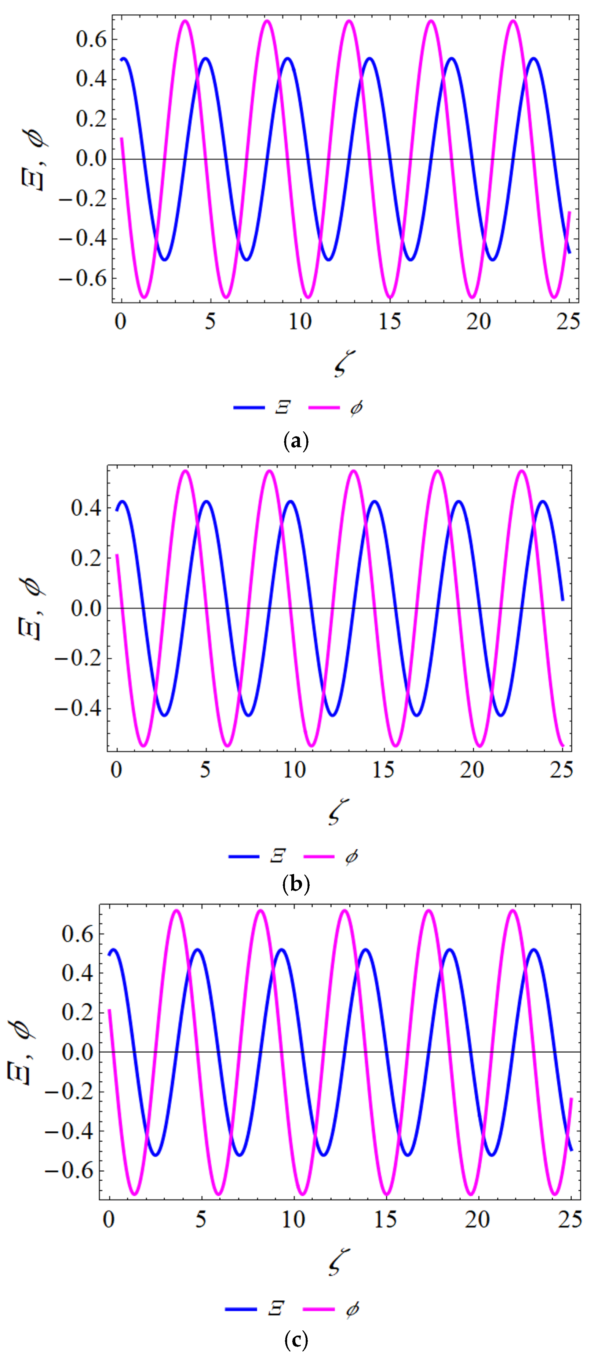
5. Results and Physical Explanation

The aim of this section is to present the extracted abundant wave solutions in Section 5 graphically and present a physical explanation.

When the parameters are assigned as $\alpha =1$, ${\beta }_1=1$, ${\beta }_2=1$, ${\epsilon }_1=1$, ${\epsilon }_2=1$, ${\mu }_1=1$, ${\mu }_2=1$, ${\kappa }_2=1$, ${\varsigma }_0=5$ and ${\eta }_0=8$, we display the behaviors of absolute value for Equation (42) under the different fractional orders $\delta =0.5$, 0.7 and 1, respectively, in Figure 4. Here, we can find the waveform is the bell-shape soliton (bright soliton), and the value of fractional order $\delta$ can influence the structure of the bright soliton; that is, the smaller its value, the more curved the wave is. With the same parameter values, the performances of the absolute value for Equation (50) with the different fractional orders $\delta =0.5$, 0.7 and 1 are unveiled in Figure 5, where it can be seen the waveform is the W-shape soliton (double-bright solitons or double bell-shaped soliton), and we can see that the smaller the value of fractional order $\delta$, the more curved the double-bright solitons become.

For $M=2$. α = 1, ${\beta }_1=1$, ${\beta }_2=1$, ${\epsilon }_1=1$, ${\epsilon }_2=1$, ${\mu }_1=1$, ${\mu }_2=1$, ${\kappa }_2=1$, ${\varsigma }_0=5$ and ${\eta }_0=8$, we describe the performances of absolute value for Equation (68) with the different fractional orders $\delta =0.5$, 0.7 and 1 in Figure 6, which indicates that the waves are all periodic waves. In addition, it can be seen that the fractional order $\delta$ can affect the waveform of the solutions; that is, the smaller the fractional order value, the more curved the contour of the periodic solution becomes.

These findings can be used to explain some wave transmission phenomena occurring in extreme environments such as irregular boundaries, fractal mediums, microgravity environment, etc.

6. Conclusions

In this article, the time-fractional chiral nonlinear Schrodinger’s equation within the conformable sense has been investigated quantitatively and qualitatively. The VP was constructed by utilizing the traveling wave transformation and the SIM. On the basis of the VP, the corresponding Hamiltonian was extracted. With the aid of the Galilean transformation, the planar dynamical system was constructed. Then, the phase portraits were depicted and the bifurcation analysis was given to discuss the existence conditions of wave solutions with different shapes. Furthermore, chaotic behaviors and a sensitivity analysis were also presented. Eventually, diverse wave solutions such as bell-shape soliton (bright soliton), W-shape soliton (double-bright solitons or double bell-shaped soliton) and periodic wave solutions were explored through two powerful approaches, the VM and HBM. These wave solutions were graphically unveiled in the form of 3D plots, 2D contour plots and 2D curves, and the influence of fractional order $\delta$ on the waveform structure of the obtained wave solutions was elaborated. The extracted wave solutions like the bell-shape soliton and the periodic wave solutions can effectively confirm discussions on the existence conditions of wave solutions with different shapes. In addition, it was found that the solution to Equation (42) was reduced into the exact solution reported in [32] for $\delta =1$ and the periodic wave solution (67) was also verified by the simple frequency amplitude formula method, thus fully confirming the correctness of the obtained solutions. As the authors know, the outcomes of this research were all new and are expected to open some new perspectives towards the dynamics of the studied equation. Furthermore, the methods and thoughts adopted in this study can also be used to probe other problems in the fields of physics and electrical and electronic engineering.

References

1. Duran, S. An investigation of the physical dynamics of a traveling wave solution called a bright soliton. Phys. Scr. 2021, 96, 125251. [Google Scholar] [CrossRef]
2. Duran, S.; Yokus, A.; Kilinc, G. A study on solitary wave solutions for the Zoomeron equation supported by two-dimensional dynamics. Phys. Scr. 2023, 98, 125265. [Google Scholar] [CrossRef]
3. Wang, K.L.; Wei, C.F. Novel optical soliton solutions to nonlinear paraxial wave model. Mod. Phys. Lett. B 2025, 39, 2450469. [Google Scholar] [CrossRef]
4. Seadawy, A.R.; Ahmad, A.; Rizvi, S.T.R.; Ahmed, S. Bifurcation solitons, Y-type, distinct lumps and generalized breather in the thermophoretic motion equation via graphene sheets. Alex. Eng. J. 2024, 87, 374–388. [Google Scholar] [CrossRef]
5. Hosseini Kamyar Mirzazadeh, M.; Baleanu, D.; Raza, N.; Park, C.; Ahmadian, A.; Salahshour, S. The generalized complex Ginzburg–Landau model and its dark and bright soliton solutions. Eur. Phys. J. Plus 2021, 136, 709. [Google Scholar]
6. Hosseini Kamyar Samadani, F.; Kumar, D.; Faridi, M. New optical solitons of cubic-quartic nonlinear Schrödinger equation. Optik 2018, 157, 1101–1105. [Google Scholar] [CrossRef]
7. Aldousari, A.; Qurban, M.; Hussain, I.; Al-Hajeri, M. Development of novel hybrid models for the prediction of COVID-19 in Kuwait. Kuwait J. Sci. 2021, 49. [Google Scholar]
8. Liu, J.-G.; Ye, Q. Stripe solitons and lump solutions for a generalized Kadomtsev-Petviashvili equation with variable coefficients in fluid mechanics. Nonlinear Dyn. 2019, 96, 23–29. [Google Scholar] [CrossRef]
9. Sohail Muhammad Naz, R.; Shah, Z.; Thounthong, P. Exploration of temperature dependent thermophysical characteristics of yield exhibiting non-Newtonian fluid flow under gyrotactic microorganisms. AIP Adv. 2019, 9, 125016. [Google Scholar] [CrossRef]
10. Wang, K.L. New computational approaches to the fractional coupled nonlinear Helmholtz equation. Eng. Comput. 2024, 41, 1285–1300. [Google Scholar] [CrossRef]
11. Wang, K.-J.; Liu, X.-L.; Wang, W.-D.; Li, S.; Zhu, H.-W. Novel singular and non-singular complexiton, interaction wave and the complex multi-soliton solutions to the generalized nonlinear evolution equation. Mod. Phys. Lett. B 2025, 39, 2550135. [Google Scholar] [CrossRef]
12. Bai, Y.S.; Zheng, L.N.; Ma, W.X.; Yun, Y.S. Hirota Bilinear Approach to Multi-Component Nonlocal Nonlinear Schrödinger Equations. Mathematics 2024, 12, 2594. [Google Scholar] [CrossRef]
13. Wang, K.J. The generalized (3+1)-dimensional B-type Kadomtsev-Petviashvili equation: Resonant multiple soliton, N-soliton, soliton molecules and the interaction solutions. Nonlinear Dyn. 2024, 112, 7309–7324. [Google Scholar] [CrossRef]
14. Ayati, Z.; Hosseini, K.; Mirzazadeh, M. Application of Kudryashov and functional variable methods to the strain wave equation in microstructured solids. Nonlinear Eng. 2017, 6, 25–29. [Google Scholar] [CrossRef]
15. Wang, K.J.; Zhu, H.W.; Shi, F.; Liu, X.L.; Wang, G.D.; Li, G. Lump wave, breather wave and the other abundant wave solutions to the (2+1)-dimensional Sawada-Kotera-Kadomtsev Petviashvili equation for fluid mechanic. Pramana 2025, 99, 40. [Google Scholar] [CrossRef]
16. Ma, W.X. A novel kind of reduced integrable matrix mKdV equations and their binary Darboux transformations. Mod. Phys. Lett. B 2022, 36, 2250094. [Google Scholar] [CrossRef]
17. Yang, D.Y.; Tian, B.; Wang, M.; Zhao, X.; Shan, W.R.; Jiang, Y. Lax pair, Darboux transformation, breathers and rogue waves of an N-coupled nonautonomous nonlinear Schrödinger system for an optical fiber or a plasma. Nonlinear Dyn. 2022, 107, 2657–2666. [Google Scholar] [CrossRef]
18. Ullah, N.; Asjad, M.I.; Hussanan, A.; Akgül, A.; Alharbi, W.R.; Algarni, H.; Yahia, I.S. Novel waves structures for two nonlinear partial differential equations arising in the nonlinear optics via Sardar-subequation method. Alex. Eng. J. 2023, 71, 105–113. [Google Scholar] [CrossRef]
19. Onder, I.; Secer, A.; Ozisik, M.; Bayram, M. On the optical soliton solutions of Kundu-Mukherjee-Naskar equation via two different analytical methods. Optik 2022, 257, 168761. [Google Scholar] [CrossRef]
20. Zhou, X.W. Exp-function method for solving Huxley equation. Math. Probl. Eng. 2008, 2008, 538489. [Google Scholar] [CrossRef]
21. Shakeel, M.; Shah, N.A.; Chung, J.D. Application of modified exp-function method for strain wave equation for finding analytical solutions. Ain Shams Eng. J. 2023, 14, 101883. [Google Scholar] [CrossRef]
22. Ma, Y.X.; Tian, B.; Qu, Q.X.; Yang, D.Y.; Chen, Y.Q. Painlevé analysis, Bäcklund transformations and traveling-wave solutions for a (3+1)-dimensional generalized Kadomtsev-Petviashvili equation in a fluid. Int. J. Mod. Phys. B 2021, 35, 2150108. [Google Scholar] [CrossRef]
23. Yin, Y.H.; Lü, X.; Ma, W.X. Bäcklund transformation, exact solutions and diverse interaction phenomena to a (3+1)-dimensional nonlinear evolution equation. Nonlinear Dyn. 2021, 108, 4181–4194. [Google Scholar] [CrossRef]
24. Zaman, U.H.M.; Arefin, M.A.; Akbar, M.A.; Uddin, M.H. Utilizing the extended tanh-function technique to scrutinize fractional order nonlinear partial differential equations. Partial. Differ. Equ. Appl. Math. 2023, 8, 100563. [Google Scholar] [CrossRef]
25. Darwish, A.; Ahmed, H.M.; Arnous, A.H.; Shehab, M.F. Optical solitons of Biswas–Arshed equation in birefringent fibers using improved modified extended tanh-function method. Optik 2021, 227, 165385. [Google Scholar] [CrossRef]
26. Zayed, E.M.E.; Alngar, M.E.M.; El-Horbaty, M.M.; Biswas, A.; Kara, A.H.; Yıldırım, Y.; Khan, S.; Alzahrani, A.K.; Belic, M.R. Cubic-quartic polarized optical solitons and conservation laws for perturbed Fokas-Lenells model. J. Nonlinear Opt. Phys. Mater. 2021, 30, 2150005. [Google Scholar] [CrossRef]
27. Akram, G.; Sadaf, M.; Khan, M.A.U. Soliton dynamics of the generalized shallow water like equation in nonlinear phenomenon. Front. Phys. 2022, 10, 822042. [Google Scholar] [CrossRef]
28. Yildirim, Y. Optical solitons of Biswas-Arshed equation by trial equation technique. Optik 2019, 182, 876–883. [Google Scholar] [CrossRef]
29. Aderyani, S.R.; Saadati, R.; Vahidi, J.; Allahviranloo, T. The exact solutions of the conformable time-fractional modified nonlinear Schrödinger equation by the Trial equation method and modified Trial equation method. Adv. Math. Phys. 2022, 2022, 4318192. [Google Scholar] [CrossRef]
30. Gkogkou, A.; Prinari, B.; Feng, B.F.; Trubatch, A.D. Inverse scattering transform for the complex coupled short-pulse equation. Stud. Appl. Math. 2022, 148, 918–963. [Google Scholar] [CrossRef]
31. Ali, M.R.; Khattab, M.A.; Mabrouk, S.M. Travelling wave solution for the Landau-Ginburg-Higgs model via the inverse scattering transformation method. Nonlinear Dyn. 2023, 111, 7687–7697. [Google Scholar] [CrossRef]
32. Eslami, M. Trial solution technique to chiral nonlinear Schrodinger’s equation in (1+ 2)-dimensions. Nonlinear Dyn. 2016, 85, 813–816. [Google Scholar] [CrossRef]
33. Hosseini, K.; Mirzazadeh, M. Soliton and other solutions to the (1+ 2)-dimensional chiral nonlinear Schrödinger equation. Commun. Theor. Phys. 2020, 72, 125008. [Google Scholar] [CrossRef]
34. Bulut, H.; Sulaiman, T.A.; Demirdag, B. Dynamics of soliton solutions in the chiral nonlinear Schrödinger equations. Nonlinear Dyn. 2018, 91, 1985–1991. [Google Scholar] [CrossRef]
35. Osman, M.S.; Baleanu, D.; Tariq, K.U.H.; Kaplan, M.; Younis, M.; Rizvi, S.T.R. Different types of progressive wave solutions via the 2D-chiral nonlinear Schrödinger equation. Front. Phys. 2020, 8, 215. [Google Scholar] [CrossRef]
36. Rezazadeh, H.; Younis, M.; Eslami, M.; Bilal, M.; Younas, U. New exact traveling wave solutions to the (2+1)-dimensional Chiral nonlinear Schrödinger equation. Math. Model. Nat. Phenom. 2021, 16, 38. [Google Scholar] [CrossRef]
37. Akinyemi, L.; Inc, M.; Khater, M.M.A.; Rezazadeh, H. Dynamical behaviour of Chiral nonlinear Schrödinger equation. Opt. Quantum Electron. 2022, 54, 191. [Google Scholar] [CrossRef]
38. Raza, N.; Javid, A. Optical dark and dark-singular soliton solutions of (1+ 2)-dimensional chiral nonlinear Schrodinger’s equation. Waves Random Complex. Media 2019, 29, 496–508. [Google Scholar] [CrossRef]
39. Al-Refai, M.; Syam, M.I.; Baleanu, D. Analytical treatments to systems of fractional differential equations with modified Atangana-Baleanu derivative. Fractals 2023, 31, 2340156. [Google Scholar] [CrossRef]
40. Alshehry, A.S.; Yasmin, H.; Ghani, F.; Shah, R.; Nonlaopon, K. Comparative analysis of advection–dispersion equations with Atangana-Baleanu fractional derivative. Symmetry 2023, 15, 819. [Google Scholar] [CrossRef]
41. Hashemi, M.S.; Mirzazadeh, M.; Ahmad, H. A reduction technique to solve the (2+ 1)-dimensional KdV equations with time local fractional derivatives. Opt. Quantum Electron. 2023, 55, 721. [Google Scholar] [CrossRef]
42. Zafar, A.; Raheel, M.; Mirzazadeh, M.; Eslami, M. Different soliton solutions to the modified equal-width wave equation with Beta-time fractional derivative via two different methods. Rev. Mex. De. Física 2022, 68. [Google Scholar] [CrossRef]
43. El-hady, E.; Ben Makhlouf, A.; Boulaaras, S.; Mchiri, L. Ulam-Hyers-Rassias stability of nonlinear differential equations with Riemann-Liouville fractional derivative. J. Funct. Spaces 2022, 2022, 7827579. [Google Scholar] [CrossRef]
44. Vishnukumar, K.S.; Vellappandi, M.; Govindaraj, V. Reachability of time-varying fractional dynamical systems with Riemann-Liouville fractional derivative. Fract. Calc. Appl. Anal. 2024, 27, 1328–1347. [Google Scholar] [CrossRef]
45. Baleanu, D.; Qureshi, S.; Yusuf, A.; Soomro, A.; Osman, M.S. Bi-modal COVID-19 transmission with Caputo fractional derivative using statistical epidemic cases. Partial. Differ. Equ. Appl. Math. 2024, 10, 100732. [Google Scholar] [CrossRef]
46. Evirgen, F. Transmission of Nipah virus dynamics under Caputo fractional derivative. J. Comput. Appl. Math. 2023, 418, 114654. [Google Scholar] [CrossRef]
47. Liang, Y.H.; Wang, K.J.; Hou, X.Z. Multiple kink soliton, breather wave, interaction wave and the travelling wave solutions to the fractional (2+1)-dimensional Boiti-Leon-Manna-Pempinelli equation. Fractal 2025, 33, 2550082. [Google Scholar] [CrossRef]
48. Chakrabarty, A.K.; Roshid, M.M.; Rahaman, M.M.; Abdeljawad, T.; Osman, M.S. Dynamical analysis of optical soliton solutions for CGL equation with Kerr law nonlinearity in classical, truncated M-fractional derivative, beta fractional derivative, and conformable fractional derivative types. Results Phys. 2024, 60, 107636. [Google Scholar] [CrossRef]
49. Wang, K.J. An effective computational approach to the local fractional low-pass electrical transmission lines model. Alex. Eng. J. 2025, 110, 629–635. [Google Scholar] [CrossRef]
50. Boulaaras, S.; Jan, R.; Khan, A.; Ahsan, M. Dynamical analysis of the transmission of dengue fever via Caputo-Fabrizio fractional derivative. Chaos Solitons Fractals X 2022, 8, 100072. [Google Scholar] [CrossRef]
51. Sousa, J.V.C.; De Oliveira, E.C. On the ψ-Hilfer fractional derivative. Commun. Nonlinear Sci. Numer. Simul. 2018, 60, 72–91. [Google Scholar] [CrossRef]
52. Aitbrahim, A.; El Ghordaf, J.; El Hajaji, A.; Hilal, K.; Valdes, J.N. A comparative analysis of Conformable, non-conformable, Riemann-Liouville, and Caputo fractional derivatives. Eur. J. Pure Appl. Math. 2024, 17, 1842–1854. [Google Scholar] [CrossRef]
53. Thabet, H.; Kendre, S. Analytical solutions for conformable space-time fractional partial differential equations via fractional differential transform. Chaos Solitons Fractals 2018, 109, 238–245. [Google Scholar] [CrossRef]
54. Li, W.-L.; Chen, S.H.; Wang, K.J. A variational principle of the nonlinear Schrödinger equation with fractal derivatives. Fractals 2025, 33, 2550069. [Google Scholar] [CrossRef]
55. Liu, J.H.; Yang, Y.N.; Wang, K.J.; Zhu, H.W. On the variational principles of the Burgers-Korteweg-de Vries equation in fluid mechanics. Europhys. Lett. 2025, 149, 52001. [Google Scholar] [CrossRef]
56. He, J.H. Semi-Inverse method of establishing generalized variational principles for fluid mechanics with emphasis on turbomachinery aerodynamics. Int. J. Turbo Jet. Engines 1997, 14, 23–28. [Google Scholar] [CrossRef]
57. Wang, K.-J.; Li, M. Variational principle of the unstable nonlinear Schrödinger equation with fractal derivatives. Axioms 2025, 14, 376. [Google Scholar] [CrossRef]
58. Liang, Y.H.; Wang, K.J. Diverse wave solutions to the new extended (2+1)-dimensional nonlinear evolution equation: Phase portrait, bifurcation and sensitivity analysis, chaotic pattern, variational principle and Hamiltonian. Int. J. Geom. Methods Mod. Phys. 2025, 22, 2550158. [Google Scholar] [CrossRef]
59. Hosseini, K.; Hinçal, E.; Ilie, M. Bifurcation analysis, chaotic behaviors, sensitivity analysis, and soliton solutions of a generalized Schrödinger equation. Nonlinear Dyn. 2023, 111, 17455–17462. [Google Scholar] [CrossRef]
60. Alizadeh, F.; Hosseini, K.; Sirisubtawee, S.; Hincal, E. Classical and nonclassical Lie symmetries, bifurcation analysis, and Jacobi elliptic function solutions to a 3D-modified nonlinear wave equation in liquid involving gas bubbles. Bound. Value Probl. 2024, 2024, 111. [Google Scholar] [CrossRef]
61. Wang, K.-J.; Zhu, H.W.; Li, S.; Shi, F.; Li, G.; Liu, X.L. Bifurcation analysis, chaotic behaviors, variational principle, Hamiltonian and diverse optical solitons of the fractional complex Ginzburg-Landau model. Int. J. Theor. Phys. 2025, 64, 134. [Google Scholar] [CrossRef]
62. Wang, K.J. Variational principle and diverse wave structures of the modified Benjamin-Bona-Mahony equation arising in the optical illusions field. Axioms 2022, 11, 445. [Google Scholar] [CrossRef]
63. He, J.H. Preliminary report on the energy balance for nonlinear oscillations. Mech. Res. Commun. 2002, 29, 107–111. [Google Scholar] [CrossRef]
Figure 1. Phase portraits for the different cases. (a) s 1 > 0 and s 2 > 0 . (b) s 1 > 0 and s 2 < 0 . (c) s 1 < 0 and s 2 > 0 . (d) s 1 < 0 and s 2 < 0 .
Axioms 14 00438 g001
Figure 2. The quasi-periodic, chaotic behaviors with α = 1 β 1 = 1 β 2 = 1 ε 1 = 1 ε 2 = 1 μ 1 = 1 μ 2 = 1 and κ 2 = 1 under the initial conditions Ξ 0 = 0.1 and ϕ 0 = 0 , (a,d) for the 2D phase portraits, (b,e) for the 3D phase portraits, (c,f) for the time series plot.
Axioms 14 00438 g002
Figure 3. Sensitivity analysis of the system with α = 1 β 1 = 1 β 2 = 1 ε 1 = 1 ε 2 = 1 μ 1 = 1 μ 2 = 1 and κ 2 = 5 at the different initial conditions (a) Ξ 0 = 0.5 ϕ 0 = 0.1 , (b) Ξ 0 = 0.4 ϕ 0 = 0.2 and (c) Ξ 0 = 0.5 ϕ 0 = 0.2 .
Axioms 14 00438 g003
Figure 4. The waveforms of ψ ± x , y , t in Equation (42) with different fractional orders δ , (ac) for δ = 0.5 , (df) for δ = 0.7 , (gi) for δ = 1 .
Axioms 14 00438 g004
Figure 5. The waveforms of ψ ± x , y , t in Equation (50) with different fractional orders δ , (ac) for δ = 0.5 , (df) for δ = 0.7 , (gi) for δ = 1 .
Axioms 14 00438 g005
Figure 6. The shapes of ψ ± x , y , t in Equation (68) with different fractional orders δ , (ac) for δ = 0.5 , (df) for δ = 0.7 , (gi) for δ = 1 .
Axioms 14 00438 g006
Disclaimer/Publisher’s Note: The statements, opinions and data contained in all publications are solely those of the individual author(s) and contributor(s) and not of MDPI and/or the editor(s). MDPI and/or the editor(s) disclaim responsibility for any injury to people or property resulting from any ideas, methods, instructions or products referred to in the content.