A Novel Robust Test to Compare Covariance Matrices in High-Dimensional Data

Abstract

The comparison of covariance matrices is one of the most important assumptions in many multivariate hypothesis tests, such as Hotelling $T^2$ and MANOVA. The sample covariance matrix, however, is singular in high-dimensional data when the variable number (p) is greater than the sample size (n). Therefore, its determinant is zero, and its inverse cannot be calculated. Although many studies addressing this problem are discussed in the Introduction Section, they have not focused on outliers in datasets. In this study, we propose a test statistic that can be used on high-dimensional datasets without being affected by outliers. There is no distributional assumption because our proposed test is permutational. We investigate the performance of the proposed test based on simulation studies and real example data. In all cases, our proposed test demonstrates good type-1 error control, power, and robustness. Additionally, we have constructed an R function and added it to the “MVTests” package. Therefore, our proposed test can be performed easily on real datasets.

1. Introduction

In many scientific disciplines, such as genomics, finance, and medical research, comparing the variability structures of multiple groups plays a crucial role in understanding group differences. In multivariate data analysis, these structures are often characterized by covariance matrices, which capture not only the spread of variables but also their mutual relationships. Before conducting comparisons of mean vectors using techniques such as the Hotelling $T^2$ test or MANOVA, it is essential to verify whether the covariance matrices across groups are homogeneous [1,2].

The assumption of homogeneity of covariance matrices, often referred to as the multivariate version of the Behrens–Fisher problem, underlies the validity of many multivariate hypothesis tests. Violations of this assumption can lead to misleading statistical conclusions. For this reason, testing the equality of covariance matrices is a fundamental problem in multivariate statistics [1].

Classical methods, such as Box’s M test [3], have long been used to assess the equality of covariance matrices. However, this test requires that the sample size be larger than the number of variables, and it is highly sensitive to outliers. As high-dimensional datasets have become increasingly common in modern research, especially when the number of variables p exceeds the sample size n, the limitations of classical approaches have become more pronounced.

In recent years, several methods have been proposed for application in high-dimensional settings. Notable among them are the tests developed by Schott [4], Srivastava and Yanagihara [5], and Li and Chen [6], which are based on Frobenius norms of covariance matrix differences. Additionally, Yu [7] introduced a permutation-based approach that does not rely on any distributional assumptions and has shown promising results for multi-sample high-dimensional comparisons.

Despite these advances, the existing methods still suffer from a major limitation: they are not robust to outliers. This study addresses this gap by proposing a novel test statistic that is applicable in high-dimensional settings and remains reliable even in the presence of outliers. Our approach is based on minimum regularized covariance determinant (MRCD) estimators [8] and utilizes a permutation-based framework, eliminating the need for distributional assumptions. The proposed method was evaluated through extensive simulation studies and a real data application to demonstrate its type-1 error control, power, and robustness.

The rest of the paper is organized as follows. Section 2 introduces the tests used to test the homogeneity of covariance matrices in high-dimensional data in the literature. In Section 3, we introduce the MRCD estimators. Section 4 introduces the proposed test procedure. Section 5 presents a simulation study to compare the type-1 error control, power, and robustness properties of the proposed approach with the $TM$ statistic proposed by Yu [7]. Section 6 exemplifies the use of the proposed approach with a real data application. Section 7 introduces the R function developed to apply the proposed approach in real data studies. Finally, Section 8 presents a discussion.

2. Literature Review

The homogeneity of variances is an important issue for inferential statistics [1,4]. In univariate mean tests (t-test or ANOVA), unequal variances are referred to as the univariate Behrens–Fisher problem. Similarly, in the Hotelling $T^2$ and MANOVA methods used for the comparison of multivariate mean vectors, there is an assumption that the variance–covariance matrices of the groups are equal [1,2]. This assumption is called the homogeneity assumption, and not meeting this assumption is called the multivariate Behrens–Fisher problem. Hypotheses about the equality of covariance matrices are established as follows:

$$\begin{array}{c}{H}_0:{\Sigma }_1={\Sigma }_2=\dots ={\Sigma }_g\\ H_1:At least {\Sigma }_j \mathrm{is} \mathrm{different} \mathrm{from} \mathrm{others}, \mathrm{j}=1,2,\dots ,\mathrm{g} \end{array}$$

(1)

where ${\Sigma }_j$ is the covariance matrix of the $j_{th}$ group, and $g$ is the number of groups. To test these hypotheses, let us draw samples with sample sizes of $n_1,n_2,\dots ,n_g$ units from multivariate normal distributions. Let the sample covariance matrices of these samples be ${\mathit{S}}_1,{\mathit{S}}_2,\dots ,{\mathit{S}}_g$, respectively. Accordingly, we can use the test statistic to test the null hypothesis given in (1):

$$U=-2\left(1-c_1\right)ln\left(M\right)~{\chi }_{{\displaystyle \frac{p\left(p+1\right)\left(g-1\right)}{2}}}^2$$

(2)

where

$$M={\displaystyle \frac{{\left|{\mathit{S}}_1\right|}^{\frac{n_1-1}{2}}{\left|{\mathit{S}}_2\right|}^{\frac{n_2-1}{2}}\dots {\left|{\mathit{S}}_g\right|}^{\frac{n_g-1}{2}}}{{\left|{\mathit{S}}_{pool}\right|}^{{{\displaystyle \sum }}_{j=1}^g\frac{n_j-1}{2}}}} , {\mathit{S}}_{pool}={\displaystyle \frac{{{\displaystyle \sum }}_{j=1}^g\left(n_j-1\right){\mathit{S}}_j}{{{\displaystyle \sum }}_{j=1}^g\left(n_j-1\right)}}$$

(3)

$$c_1=\left\{\begin{array}{cc}\left[{\displaystyle \frac{2p^2+3p-1}{6\left(p+1\right)\left(g-1\right)}}\right]\left[{\displaystyle \sum }_{j=1}^g{\displaystyle \frac{1}{n_j-1}}-{\displaystyle \frac{1}{{{\displaystyle \sum }}_{j=1}^g\left(n_j-1\right)}}\right] ,& \exists \left(n_i\ne n_j\right), i\ne j=1,2,\dots ,g\\ \left[{\displaystyle \frac{\left(g+1\right)\left(2p^2+3p-1\right)}{6g\left(p+1\right)\left(n-1\right)}}\right] ,& n_1=n_2=\dots =n_g=n\end{array}\right..$$

(4)

When $U>{\chi }_{{\displaystyle \frac{p\left(p+1\right)\left(g-1\right)}{2}};\alpha }^2$, we reject the null hypothesis [1,2]. However, the test statistic given in Equation (2) can be only used for low-dimensional data where $p<min\left\{n_1,n_2,\dots ,n_g\right\}$ and the samples come from multivariate normal distribution [3].

In addition to hypothesis testing procedures, recent studies have focused on improving covariance matrix estimation in high-dimensional settings. Among these, shrinkage-based estimators have attracted particular attention due to their ability to produce well-conditioned covariance estimates when the number of variables exceeds the sample size. Ledoit and Wolf [9] introduced a linear shrinkage estimator that combines the sample covariance matrix with a structured target to stabilize estimation. Similarly, Schäfer and Strimmer [10] proposed a shrinkage approach particularly suited to applications in genomics and functional data analysis. Although our study focuses on hypothesis testing, incorporating such estimation techniques can improve the reliability of test statistics in challenging high-dimensional scenarios.

Several tests have been proposed to test hypotheses about the equality of covariance matrices in high-dimensional data [4,5,6,7,11]. Schott [4] and Srivastava and Yanagihara [5] have suggested tests to compare any two covariance matrices based on the Frobenius norm. Similarly, Li and Chen [6] proposed a test statistic based on Frobenius norm to test the hypothesis about the equality of two covariance matrices of two independent high-dimensional groups. Their test statistic is given in Equation (5).

$$T_{n_1,n_2}=A_{n_1}+A_{n_2}-2C_{n_1{n}_2}$$

(5)

where, under the assumption that ${\mathit{\mu }}_1={\mathit{\mu }}_2=0$, we can calculate the $A_{n_h}$ $\left(h=1,2\right)$ and $C_{n_1{n}_2}$ values as follows:

$$A_{n_h}={\displaystyle \frac{1}{n_h\left(n_h-1\right)}}{\displaystyle \sum }_{i\ne j}{\left(X_{hi}^{\prime }{X}_{hj}\right)}^2, C_{n_1{n}_2}={\displaystyle \frac{1}{n_1{n}_2}}{\displaystyle \sum }_i{\displaystyle \sum }_j{\left(X_{1i}^{\prime }{X}_{2j}\right)}^2.$$

(6)

Li and Chen [6] defined the asymptotic distribution of $T_{n_1,n_2}$ statistic under the null hypothesis $H_0:{\Sigma }_1={\Sigma }_2=\Sigma$ as follows:

$${\displaystyle \frac{T_{n_1,n_2}}{{\widehat{\sigma }}_{n_1,n_2}}}~N\left(0,1\right), {\hat{\sigma }}_{n_1,n_2}^2=4{\left({\displaystyle \frac{1}{n_1}}+{\displaystyle \frac{1}{n_2}}\right)}^{2}t{r}^2\left({\Sigma }^2\right).$$

(7)

This test proposed by Li and Chen [6] can test the null hypothesis given in (1) when the number of groups is two. To solve this problem, Wang [11] proposed to divide the null hypothesis given in (1) into $g-1$ pieces and to use the $T_{n_1,n_2}$ statistic defined in Equation (5) to test these hypotheses. For this purpose, we can rewrite the null hypothesis in (1) as $H_0=H_{02}\cap H_{03}\cap \dots \cap H_{0g}$, where the $H_{0j}$ and $H_{1j}$ hypotheses can be written as follows:

$$H_{0j}:{\Sigma }_{j-1}={\Sigma }_j \mathrm{vs}. H_{1j}:{\Sigma }_{j-1}\ne {\Sigma }_j , j=2,3,\dots ,g.$$

(8)

Because there are g − 1 comparisons, we use the Bonferroni correction. Accordingly, the test is performed according to the largest of the calculated $T_{j-1,j} \left(j=2,\dots ,g\right)$ statistics by absolute value. If the null hypothesis cannot be rejected according to this statistic, then that the null hypothesis given by (1) cannot be rejected.

Yu [7] suggested a permutation test to compare covariance matrices and to test the null hypothesis in Equation (1) in high-dimensional datasets. Let ${\mathit{S}}_j$ be the sample covariance matrix of the $j_{th}$ group $\left(j=1,2,\dots ,g\right)$. The pooled covariance matrix can be calculated as follows:

$${\mathit{S}}_{pool}={\displaystyle \frac{{{\displaystyle \sum }}_{j=1}^g{n}_j{\mathit{S}}_j}{{{\displaystyle \sum }}_{j=1}^g{n}_j}}.$$

(9)

If the mean vectors of the groups are zero vectors, $M_{hk}$ can be used for the pairwise comparison of the covariance matrices of the $h_{th}$ and $k_{th}$ groups. We can define $M_{hk}$ as follows:

$$M_{hk}=max\left\{\left|{\lambda }_1,{\lambda }_2,\dots ,{\lambda }_s\right|\right\}$$

(10)

where ${\lambda }_1,{\lambda }_2,\dots ,{\lambda }_s$ are non-zero eigenvalues of the matrix $\sqrt{{\displaystyle \frac{n_h{n}_k}{n}}}{\mathit{S}}_{pool.d}^{-1/2}\left({\mathit{S}}_h-{\mathit{S}}_k\right){\mathit{S}}_{pool.d}^{-1/2}$, and ${\mathit{S}}_{pool.d}$ is a diagonal matrix and has the same diagonal elements as ${\mathit{S}}_{pool}$. Yu [7] proposed the following test statistic:

$$T{M}_{YU}={\displaystyle \frac{2}{g\left(g-1\right)}}{\displaystyle \sum }_{h<k}{M}_{hk}.$$

(11)

Because the distribution of the $T{M}_{YU}$ statistic is not known, Yu [7] proposed using a permutation approach to obtain the sampling distribution of the test statistic. Detailed information is available in [7].

All of the approaches introduced above are sensitive to outliers in the dataset since they are based on classical estimations. This study aims to propose a test statistic to compare the covariance matrices of $g$-independent groups in high-dimensional data contaminated with outliers. The proposed test statistic is based on the minimum regularized covariance determinant (MRCD) estimations introduced in Section 3. Details of these estimations are given in Section 4.

3. MRCD Estimators

Outliers in multivariate data can significantly distort classical estimates of location and dispersion. The minimum covariance determinant (MCD) estimator is a robust alternative that is less sensitive to outliers. This makes it ideal to estimate the location and scatter parameters in contaminated data. However, MCD estimates cannot be used in high-dimensional data where the number of variables $\left(p\right)$ exceeds the sample size $\left(n\right)$. This limitation restricts its applicability in high-dimensional data.

Boudt et al. [8] proposed minimum regularized covariance determinant (MRCD) estimators of location and scatter parameters without being affected by outliers in high-dimensional data. The MRCD estimator retains the good breakdown point properties of the MCD estimator [8,12].

To compute MRCD estimates, we first standardized the data using the median and $Q_n$ as the univariate location and scatter estimators [13], and then used the $\mathit{T}$ target matrix. This $\mathit{T}$ matrix was symmetric and positive definite. The regularized covariance matrix of any subset $H$ obtained from the standardised $\mathit{Z}$ data was computed as follows:

$$\mathit{K}\left(H\right)=\rho \mathit{T}+\left(1-\rho \right)c_{\alpha }{\mathit{S}}_Z\left(H\right)$$

(12)

where $\rho$ is the regularization parameter, $c_{\alpha }$ is the consistency factor defined by Croux and Haesbroeck [14], and

$${\mathit{S}}_Z\left(H\right)={\displaystyle \frac{1}{h-1}}{\left({\mathit{Z}}_H-{\mathit{\mu }}_Z\left(H\right)\right)}^T\left({\mathit{Z}}_H-{\mathit{\mu }}_Z\left(H\right)\right) ,{\mathit{\mu }}_Z\left(H\right)={\displaystyle \frac{1}{h}}{\mathit{Z}}_H^T{1}_h.$$

(13)

MRCD estimations are obtained from the subset $H_{MRCD}$, which is obtained by solving the minimization problem given by Equation (14).

$$H_{MRCD}=\underset{H\in \mathcal{H}}{\mathrm{argmin}}\left[det{\left(\mathit{K}\left(H\right)\right)}^{1/p}\right]$$

(14)

where $\mathcal{H}$ is the set of all subsets with size $h$ in the data. Finally, the MRCD location and scatter estimators were obtained as given in Equations (15) and (16).

$${\hat{\mu }}_{MRCD}={\mathit{V}}_X+{\mathit{D}}_X {\mathit{\mu }}_Z\left(H_{MRCD} \right)$$

(15)

$${\hat{\Sigma }}_{MRCD}={\mathit{D}}_X \mathit{Q}{\Lambda }^{1/2}\left[\rho \mathit{I}+\left(1-\rho \right)c_{\alpha }{\mathit{S}}_w\left(H_{MRCD}\right)\right]{\Lambda }^{1/2}{\mathit{Q}}^{\prime }{\mathit{D}}_X$$

(16)

where $\Lambda$ and $\mathit{Q}$ are the eigenvalues and eigenvector matrices of $T$, respectively. Also, ${\mathit{S}}_w\left(H_{MRCD}\right)$ was calculated as follows:

$${\mathit{S}}_w\left(H_{MRCD}\right)={\Lambda }^{-1/2}{\mathit{Q}}^{\prime }{\mathit{S}}_Z\left(H_{MRCD}\right)\mathit{Q}{\Lambda }^{-1/2}.$$

(17)

More detailed information on the MRCD estimators can be found in [8]. In this study, we used the “rrcov” package in R software for calculations regarding the MRCD estimators [15]. When using this package, we assumed that we knew the outlier rate of the data. We also preferred to use the default values of the regularization parameter (rho) and the target matrix. This function automatically calculates these values from the dataset.

4. Proposed Test Statistic

To test the equality of covariance matrices in high-dimensional data, the test statistics given by Equations (10) and (11) have been shown to be more successful than alternative methods [7]. However, since these test statistics are based on classical covariance matrices, they are affected by outliers in the dataset. Moreover, the ${\mathit{S}}_{pool.d}$ matrix used in these test statistics is a diagonal matrix consisting of the ${\mathit{S}}_{pool}$ covariance matrix. Therefore, it only considers the variances of the variables and excludes the relationships among the variables.

In this study, to test the null hypothesis given by (1) in contaminated high-dimensional data, we propose using the MRCD estimators introduced in Section 2 instead of the classical estimators in the test statistics given by Equations (10) and (11). We also recommend using the ${\mathit{S}}_{pool}^{-1/2}$ matrix directly instead of the ${\mathit{S}}_{pool.d}^{-1/2}$ matrix to take the relationships among the variables into account in the test statistics. In the proposed approach, the ${\mathit{S}}_{pool}^{1/2}$ matrix can be calculated by using spectral decomposition as follows:

$${\mathit{S}}_{pool}={\mathit{S}}_{pool}^{1/2}{\mathit{S}}_{pool}^{1/2}$$

(18)

$${\mathit{S}}_{pool}^{1/2}=\mathit{P}{\Lambda }^{1/2}{\mathit{P}}^T$$

(19)

where $\Lambda$ is the diagonal eigenvalue matrix of ${\mathit{S}}_{pool}$, and $P$ is the orthogonal eigenvector matrix. We calculated the ${\mathit{S}}_{pool}$ matrix based on the MRCD estimations, as given in Equation (20).

$${\mathit{S}}_{pool}={\displaystyle \frac{{{\displaystyle \sum }}_{h=1}^g{n}_h{\mathit{S}}_{MRCD.h}}{{{\displaystyle \sum }}_{h=1}^g{n}_h}}$$

(20)

where ${\mathit{S}}_{MRCD.h}$ is the MRCD covariance matrix of the $h_{th}$ group $\left(h=1,2,\dots ,g\right)$.

If the mean vectors of the groups are zero vector, $M_{hk}^{\prime }$ can be used for pairwise comparison of the covariance matrices of the $h_{th}$ and $k_{th}$ groups as follows:

$$M_{hk}^{\prime }=max\left\{\left|{\lambda }_1,{\lambda }_2,\dots ,{\lambda }_s\right|\right\}$$

(21)

where ${\lambda }_1,{\lambda }_2,\dots ,{\lambda }_s$ are the non-zero eigenvalues of the matrix $\sqrt{{\displaystyle \frac{n_h{n}_k}{n}}}{\mathit{S}}_{pool}^{-1/2}\left({\mathit{S}}_h-{\mathit{S}}_k\right){\mathit{S}}_{pool}^{-1/2}$, and ${\mathit{S}}_{pool}$ is calculated as given in Equation (20). We propose the following test statistic to test the null hypothesis given in (1):

$$T{M}_{MRCD}={\displaystyle \frac{2}{g\left(g-1\right)}}{\displaystyle \sum }_{h<k}{M}_{hk}^{\prime }.$$

(22)

Because the distribution of the $T{M}_{MRCD}$ statistic is not known, we can use a permutation approach to obtain the sampling distribution of the test statistic as proposed by Yu [7]. For this purpose, we propose the following Algorithm 1 to test the null hypothesis:

Algorithm 1: Robust test for comparison of covariance matrices

Let ${\mathit{X}}_{hi}$ be the $i_{th} \left(i=1,2,\dots ,n_h\right)$ observation vector in the $h_{th}$ group $\left(h=1,2,\dots ,g\right)$. Combine all ${\mathit{X}}_{hi}$ observation vectors to the data ${\mathit{X}}_{n\times p}$. Randomly distribute the observations in the data ${\mathit{X}}_{n\times p}$ into $g$ groups such that there are $n_h$ observations in the $h_{th}$ group. After this operation, let ${\mathit{X}}_{hi}^{\left(1\right)}$ represent the $n_h$ observations in the $h_{th}$ group. For each group, calculate the MRCD covariance matrices ${\mathit{S}}_{MRCD.h}$ $\left(h=1,2,\dots ,g\right)$ based on the ${\mathit{X}}_{hi}^{\left(1\right)}$ observations and calculate the statistic given by Equation (22). Let us denote this statistic as $T{M}_{MRCD}^{\left(1\right)}$. Repeat steps (i)–(iii) $R$ times and calculate the statistics $T{M}_{MRCD}^{\left(r\right)}$ $\left(r=1,2,\dots ,R\right)$ at each step. Calculate the p-value as follows:         $p-value=\#\left\{r: T{M}_{MRCD}^{\left(r\right)}>T{M}_{MRCD}\right\}/R .$

When the p-value is lower than the significance level, the null hypothesis given by (1) is rejected, indicating that the covariance matrices are not homogeneous.

If the mean vectors are not equal to the zero vectors, then the test statistic given by Equality (22) is defined as follows:

$$T{M}_{MRCD}={\displaystyle \frac{2}{g\left(g-1\right)}}{\displaystyle \sum }_{h<k}max\left\{\left|eigenvalues of \sqrt{{\displaystyle \frac{n_h{n}_k}{n}}}\left({\mathit{S}}_{MRCD.h}-{\mathit{S}}_{MRCD.k}\right) \right|\right\}$$

(23)

where ${\mathit{S}}_{\mathit{M}RCD.h}={\displaystyle \frac{1}{n_h}}{\displaystyle \sum }_{i=1}^{n_h}{\mathit{Z}}_{hi}{\left({\mathit{Z}}_{hi}\right)}^T,{\mathit{Z}}_{hi}={\mathit{S}}_{pool}^{-1/2}\left({\mathit{X}}_{hi}-{\overline{\mathit{X}}}_h\right).$ ${\mathit{S}}_h={\displaystyle \frac{1}{n_h}}{\displaystyle \sum }_{i=1}^{n_h}{\mathit{Z}}_{hi}{\left({\mathit{Z}}_{hi}\right)}^T$, ${\mathit{Z}}_{hi}={\mathit{S}}_{pool.d}^{-1/2}\left({\mathit{X}}_{hi}-{\mathit{M}}_h\right)$, and ${\left(.\right)}^T$ is the transpose operator. Here, ${\mathit{S}}_{pool}$ is calculated as given in Equation (20), and ${\mathit{M}}_h$ is the MRCD location estimation of the $h_{th}$ group.

Lemma 1.

Let $b$ be the number of test statistics computed from $R$ randomly sampled permutations (without replacement) that are more extreme than the observed test statistic  $T{M}_{MRCD}$. Then, the p-value defined as

$$p={\displaystyle \frac{b}{R}}$$

(24)

is a consistent estimator under the null hypothesis and converges to the true significance level as $R\to \infty$, provided that the permutation distribution approximates the true null distribution. □

This formulation aligns with the permutation-based inference strategy described by Yu [7] and is widely used in the literature for high-dimensional testing problems. Although alternatives, such as $\left(b+1\right)/\left(R+1\right),$ have been proposed [16] to avoid zero p-values and improve small-sample behavior, we did not observe any zero p-values in our simulation settings. Thus, the classical estimator $b/R$ remains practically appropriate and computationally efficient in our context.

The test we propose can test whether the covariance matrices of high-dimensional independent groups are equal or not without being affected by outliers in the dataset. Moreover, since it is a permutation test, it does not require any distributional assumption.

The proposed test statistic $T{M}_{MRCD}$ integrates a robust covariance estimation approach (MRCD) with a permutation-based inference strategy. This design grants the test several important theoretical properties:

• Nonparametric nature: The test does not require multivariate normality. Its null distribution is derived empirically via permutation of the group labels. Under the null hypothesis and assuming exchangeability, this ensures exact control of type-1 error in finite samples.
• Robustness to outliers: Unlike the TM_YU test, the TM_MRCD test based on MRCD estimations is robust to outliers in data. The MRCD estimator, while not affine equivariant due to the use of a fixed regularization matrix, offers strong resistance to outliers. It guarantees a minimum eigenvalue bounded away from zero when the regularization parameter is applied, resulting in a 100% implosion breakdown value [8]. Though not maximally robust in all directions, this feature provides practical protection against severe contamination.
• Finite sample validity: Since permutation testing is used, type-1 error control holds in finite samples, making the procedure reliable even for small sample sizes, provided that the group labels are exchangeable.
• Asymptotic behavior: Although a formal proof of asymptotic consistency is beyond the scope of this paper, the simulation results show that the type-1 error rates stabilize near the nominal level as the sample size increases. This is consistent with findings from the permutation test literature.
• High-dimensional applicability: Unlike Box’s M test, which fails in high-dimensional contexts, TM_MRCD remains valid and operational. This makes it suitable for applications such as gene expression analysis, where the number of variables often exceeds the sample size.

These properties make $T{M}_{MRCD}$ a robust and flexible tool for covariance matrix comparison in challenging data environments.

5. Simulation Study

In this section, we perform simulation studies to compare our statistics with the $TM$ statistic proposed by Yu [7] and the $M$ statistic suggested by Box [3]. Since the $M$ statistic can only be used for low-dimensional data, it is not included in the comparisons for high-dimensional data. In the simulation studies, we compared the test statistics according to the type-1 error, power, and robustness performance. The significance level was $\alpha =0.05$ for all tests. Although these test statistics can measure the covariance matrix of two or more groups, only three group covariance matrices were compared in the simulation studies. In other words, each test evaluated the null hypothesis $H_0:{\Sigma }_1={\Sigma }_2={\Sigma }_3$.

In the simulation study, the sample sizes of the groups were taken as equal to each other. Accordingly, the sample sizes $\left(n_h\right)$ were taken as 10, 30, and 60. The number of variables $\left(p\right)$ was determined as 5, 10, 50, 100, and 300. Therefore, both low-dimensional and high-dimensional data were included in the dataset used in simulation studies. In each step of the simulation study, the number of trials $\left(R\right)$ was taken as 1000 repetitions.

5.1. Comparisons of Type-1 Error Rates

To investigate the type-1 error performance of our proposed test, we compared the rejection rates when the null hypothesis which was true. Similar to the simulation study used by Yu [7], the diagonal elements of the ${\Sigma }_1$ matrix were ${\sigma }_{1ii}=1 \left(i=1,2,\dots ,p\right),$ and its non-diagonal elements were ${\sigma }_{1ij}={0.6}^{\left|i-j\right|} \left(i\ne j=1,2,\dots ,p\right)$. In order for the null hypothesis to be true, we defined the other covariance matrices as ${\Sigma }_2={\Sigma }_3={\Sigma }_1$.

We generated datasets under two scenarios: multivariate normal distribution and mixed distributions. We give details about these scenarios below. To make more precise comparisons in terms of type-1 error, the average relative error (ARE) values were calculated for each statistic. The ARE values indicate the deviation of the test statistic from the nominal significance level of type-1 proportions and were calculated as given in Equation (25).

$$ARE={\displaystyle \frac{100}{\theta \alpha }}{\displaystyle \sum }_{i=1}^{\theta }\left|{\hat{\alpha }}_i-\alpha \right|.$$

(25)

where $\theta$ is the number of type-1 error rates calculated for each statistic in the table, ${\hat{\alpha }}_i$ is the number of type-1 error rates, and $\alpha$ is the nominal significance level used in the testing process. In this study, we used the significant level $\alpha$ as 5%. We can say that the test statistic with the smallest ARE value had a higher performance in terms of the type-1 error rate.

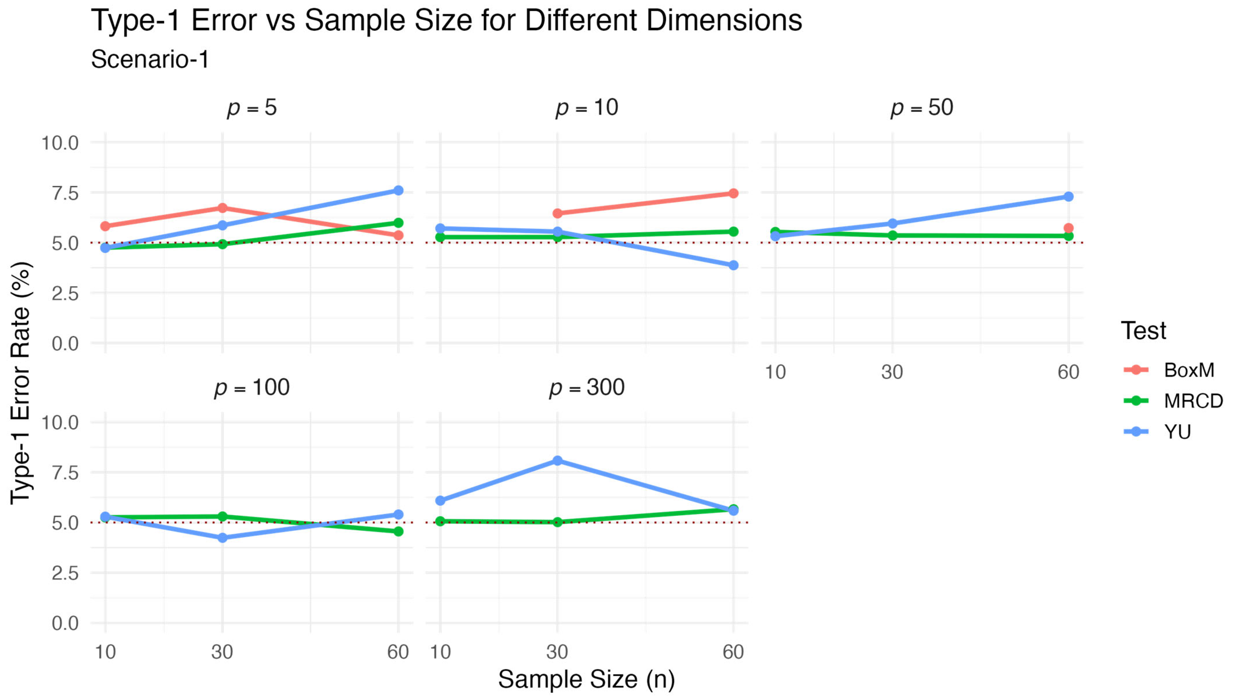
• Scenario 1: We generated datasets from multivariate normal distribution. For this purpose, the mean vectors were set as ${\mu }_1={\mu }_2={\mu }_3=0$ without any loss of generality. Accordingly, observations in each group were randomly generated from $X_h~N_p\left({\mu }_h,{\Sigma }_h\right) \left(h=1,2,3\right),$ such that the sample sizes were $n_h=10, 30, 60$. We tested the null hypothesis $H_0:{\Sigma }_1={\Sigma }_2={\Sigma }_3,$ which is true in this case. The obtained results are presented in

  Table 1. Type-1 error rates of methods based on normally distributed data.

  ${\mathit{n}}_{\mathit{h}}$	p	$\mathit{T}{\mathit{M}}_{\mathit{M}\mathit{R}\mathit{C}\mathit{D}}$	$\mathit{T}{\mathit{M}}_{\mathit{Y}\mathit{U}}$	$\mathit{M}$
  10	5	4.751	4.738	5.818
  30	5	4.923	5.861	6.727
  60	5	5.987	7.603	5.364
  10	10	5.275	5.709	-
  30	10	5.276	5.549	6.455
  60	10	5.549	3.874	7.455
  10	50	5.533	5.319	-
  30	50	5.359	5.955	-
  60	50	5.333	7.294	5.727
  10	100	5.255	5.290	-
  30	100	5.299	4.236	-
  60	100	4.554	5.398	-
  10	300	5.061	6.088	-
  30	300	5.017	8.081	-
  60	300	5.661	5.588	-
  ARE:		7.171	21.182	25.152

  and visualized in Figure 1.

The results presented in Table 1 and illustrated in Figure 1 show the behaviors of the three test statistics in terms of type-1 error control under various sample sizes and dimensional settings. The proposed $T{M}_{MRCD}$ test consistently yielded rejection rates that were closest to the nominal 5% level across all considered scenarios. This accuracy is reflected in its notably lower average relative error (ARE) compared to the alternative methods. In contrast, $T{M}_{YU}$ tended to deviate from the nominal level, especially for higher values of $p$, while Box’s M test was applicable only in low-dimensional settings and exhibited greater variability. The graphical representation reinforces these numerical findings and highlights the comparative advantage of the proposed test in controlling the type-1 error rate under Scenario 1.

• Scenario 2: The mixed distribution data in this scenario were generated in two stages, as follows:
  • The observation vectors ${\mathit{Z}}_{hi}={\left[Z_{hi1},Z_{hi2},\dots ,Z_{hip}\right]}^T$ were generated. Here, the first $p_1=p/2$ variables came from the standardized normal distribution $N\left(0,1\right)$, and the remaining $p_2=p-p_1$ variables came from the standardized chi-square distribution $\left({\chi }_2^2-2\right)/2$.
  • The ${\mathit{X}}_{hi}$ observation vectors $\left(i=1,2,\dots ,n_h\right)$ were obtained with the transformation ${\mathit{X}}_{hi}={\Sigma }_h^{1/2}{Z}_{hi}$ $\left(h=1,2,3\right)$. The ${\mathit{X}}_{hi}$ observations had a mean vector of $0$ and a covariance matrix ${\Sigma }_h$.

After the datasets were generated in this way, we tested the null hypothesis ${\mathrm{H}}_0:{\Sigma }_1={\Sigma }_2={\Sigma }_3$, which is actually true. The $p$, $n_h,$ and ${\Sigma }_h$ values used here correspond to those given in Scenario 1. The results are presented in

Table 2. Type-1 error rates of methods based on mixed distributed data.

${\mathit{n}}_{\mathit{h}}$	p	$\mathit{T}{\mathit{M}}_{\mathit{M}\mathit{R}\mathit{C}\mathit{D}}$	$\mathit{T}{\mathit{M}}_{\mathit{Y}\mathit{U}}$	$\mathit{M}$
10	5	5.153	5.151	27.455
30	5	5.618	5.554	27.727
60	5	5.100	6.182	29.364
10	10	5.814	5.171	-
30	10	5.044	5.445	26.091
60	10	5.509	5.057	26.636
10	50	4.928	5.538	-
30	50	5.200	4.800	-
60	50	5.362	5.759	27.818
10	100	5.400	4.940	-
30	100	5.296	5.783	-
60	100	5.158	6.080	-
10	300	5.419	5.506	-
30	300	5.514	4.851	-
60	300	5.031	5.684	-
ARE:		6.254	9.758	180.121

and visualized in Figure 2.

The simulation results under the mixed distributed data are summarized in Table 2 and visualized in Figure 2. The $T{M}_{MRCD}$ statistic continued to exhibit robust performance in controlling the type-1 error rate, yielding rejection rates that remained consistently close to the nominal level across all combinations of n and p. This is reflected in the lowest ARE value (6.254) among the three methods. The $T{M}_{YU}$ test also performed reasonably well in this setting, with moderate deviations from the nominal 5% level, particularly at higher dimensions. In contrast, the classical Box’s M test showed severe inflation of type-1 error rates under the mixed distribution, with values exceeding 25% in all applicable scenarios. For this reason, the Box M test was excluded from Figure 2 to improve the readability and visual interpretability of the results.

In both Figure 1 and Figure 2, the horizontal dashed line represents the nominal 5% significance level; test statistics with values closer to this line are considered more accurate in terms of type-1 error control.

5.2. Comparison of Powers

To examine the power performance of the proposed approach, we compared the rejection rates when the null hypothesis was false. Similar to the simulation design used by Yu [7], the ${\Sigma }_1$ matrix was defined as shown in Section 5.1. However, we defined ${\Sigma }_2=2{\Sigma }_1$ and ${\Sigma }_3=10{\Sigma }_1$ to ensure the null hypothesis was false. Datasets were generated under two different scenarios: multivariate normal distribution and mixed.

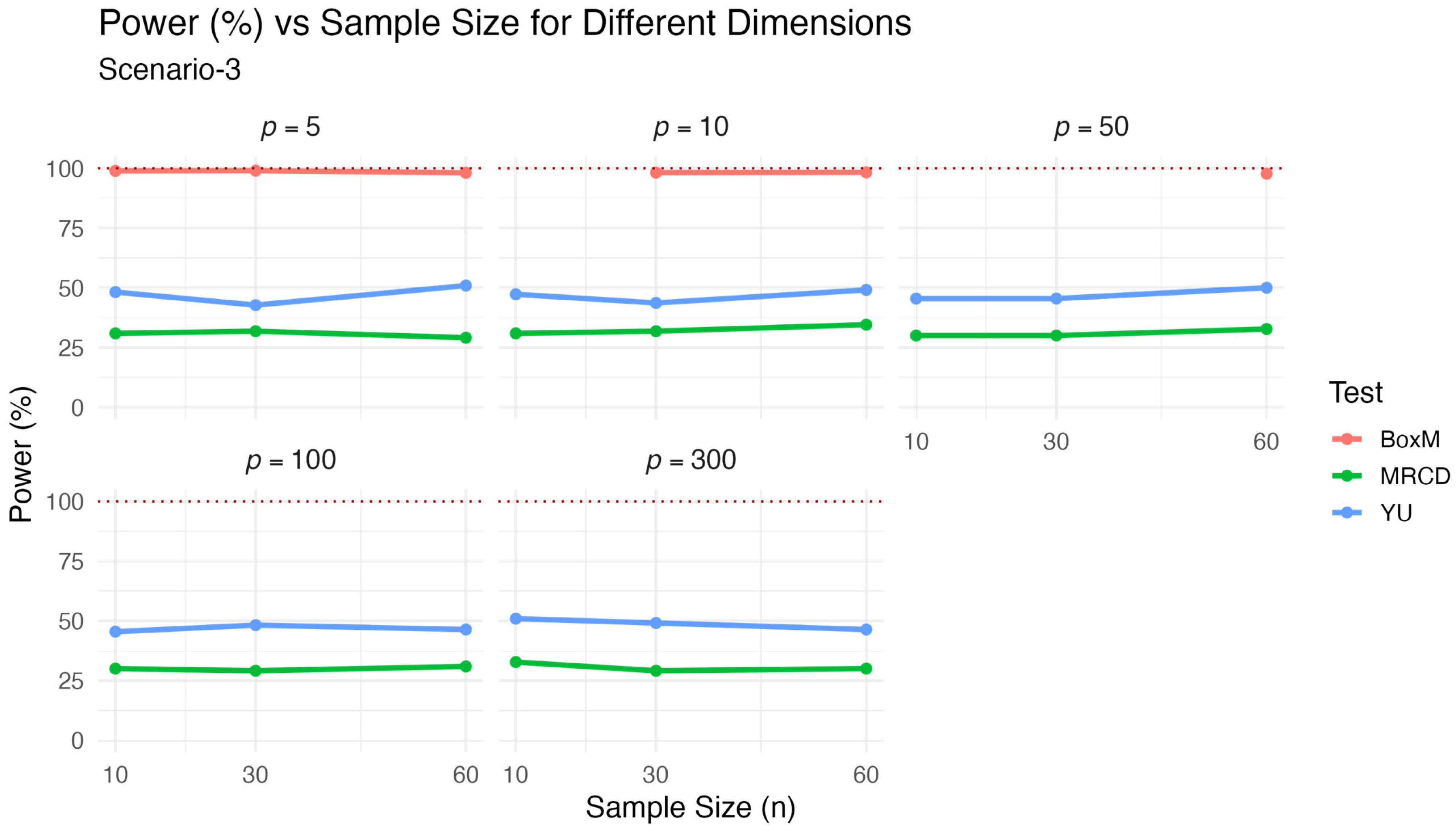
• Scenario 3: We generated datasets from a multivariate normal distribution. For this purpose, the mean vectors were set as ${\mu }_1={\mu }_2={\mu }_3=0$ without any loss of generality. Accordingly, observations in each group were randomly generated from $X_h~N_p\left({\mu }_h,{\Sigma }_h\right) \left(h=1,2,3\right)$ such that the sample sizes were $n_h=10, 30, 60$. We tested the null hypothesis $H_0:{\Sigma }_1={\Sigma }_2={\Sigma }_3$, which is false. The power performance of the test statistics under multivariate normal distribution is presented in

  Table 3. Powers of methods based on normally distributed data.

  ${\mathit{n}}_{\mathit{h}}$	p	$\mathit{T}{\mathit{M}}_{\mathit{M}\mathit{R}\mathit{C}\mathit{D}}$	$\mathit{T}{\mathit{M}}_{\mathit{Y}\mathit{U}}$	$\mathit{M}$
  10	5	30.909	48.182	98.909
  30	5	31.818	42.727	99.000
  60	5	29.091	50.909	98.091
  10	10	30.909	47.273	-
  30	10	31.818	43.636	98.182
  60	10	34.545	49.091	98.273
  10	50	30.000	45.455	-
  30	50	30.000	45.455	-
  60	50	32.727	50.000	97.727
  10	100	30.000	45.455	-
  30	100	29.091	48.182	-
  60	100	30.909	46.364	-
  10	300	32.727	50.909	-
  30	300	29.091	49.091	-
  60	300	30.000	46.364	-

  and visualized in Figure 3.

As expected, the classical Box’s M test yielded the highest power values across all scenarios, often exceeding 95%. However, this high power comes at the cost of poor type-1 error control in high-dimensional or non-normal data, as shown in previous results. The $T{M}_{YU}$ test exhibited moderately high power, typically ranging between 43% and 51%, and remained relatively stable across dimensions. The proposed $T{M}_{MRCD}$ test demonstrated the lowest power values among the three, generally around 30%, but still consistent across varying sample sizes and dimensions. These results reflect the classical trade-off between power and robustness: while $T{M}_{MRCD}$ is more conservative, it provides strong type-1 error control even in contaminated or non-normal data settings. Therefore, although its power is slightly lower, it offers a more reliable alternative when robustness is essential.

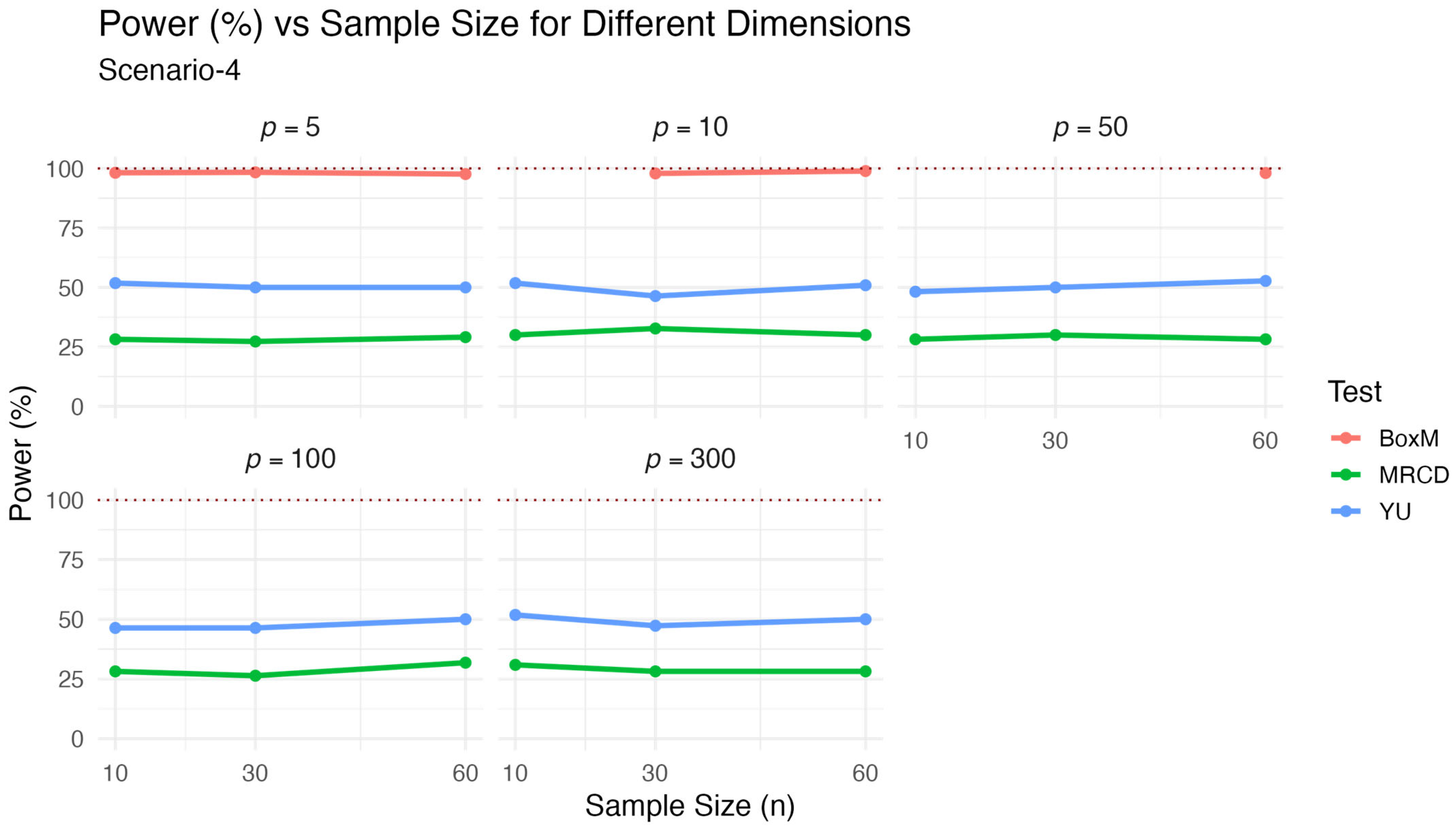
• Scenario 4: In this scenario, we generated observations as defined in Scenario 2. Unlike in Scenario 2, the ${\Sigma }_h \left(h=1,2,3\right)$ matrices were different from each other here. After the datasets were generated in this way, we tested the null hypothesis $H_0:{\Sigma }_1={\Sigma }_2={\Sigma }_3$ which is actually false. The p, $n_h,$ and ${\Sigma }_h$ values used here were as given in Scenario 3. The results are presented in

  Table 4. Powers of methods based on mixed distributed data.

  ${\mathit{n}}_{\mathit{h}}$	p	$\mathit{T}{\mathit{M}}_{\mathit{M}\mathit{R}\mathit{C}\mathit{D}}$	$\mathit{T}{\mathit{M}}_{\mathit{Y}\mathit{U}}$	$\mathit{M}$
  10	5	28.182	51.818	98.182
  30	5	27.273	50.000	98.364
  60	5	29.091	50.000	97.636
  10	10	30.000	51.818	-
  30	10	32.727	46.364	97.909
  60	10	30.000	50.909	98.909
  10	50	28.182	48.182	-
  30	50	30.000	50.000	-
  60	50	28.182	52.727	98.091
  10	100	28.182	46.364	-
  30	100	26.364	46.364	-
  60	100	31.818	50.000	-
  10	300	30.909	51.818	-
  30	300	28.182	47.273	-
  60	300	28.182	50.000	-

  and visualized in Figure 4.

The results for Scenario 4, which involved mixed distributed data under the alternative hypothesis, are presented in Table 4 and visualized in Figure 4. Similar to the previous scenario, Box’s M test showed the highest power values, often exceeding 97%, but its known sensitivity to distributional deviations limits its practical reliability. The $T{M}_{YU}$ test maintained stable and moderately high power across varying dimensionalities and sample sizes, typically around 50%. The proposed $T{M}_{MRCD}$ test again demonstrated lower power, generally between 26% and 32%, but its behavior remained consistent across the simulation settings. These results align with the classical robustness–power trade-off, where $T{M}_{MRCD}$ prioritizes robustness and type-1 control over maximizing power. While the power of the proposed test was lower in this contaminated data scenario, its performance did not substantially deteriorate, suggesting resilience under non-ideal conditions.

5.3. Comparisons of Robustness

In order to examine the robustness of the proposed approach to outliers, we first contaminated the dataset and then calculated the rejection rates of the null hypothesis, which is true. The observations generated here can be categorized as regular and outliers. Here, too, the data were contaminated with two different scenarios. In each case, the covariance matrices were generated as those given in Section 5.1.

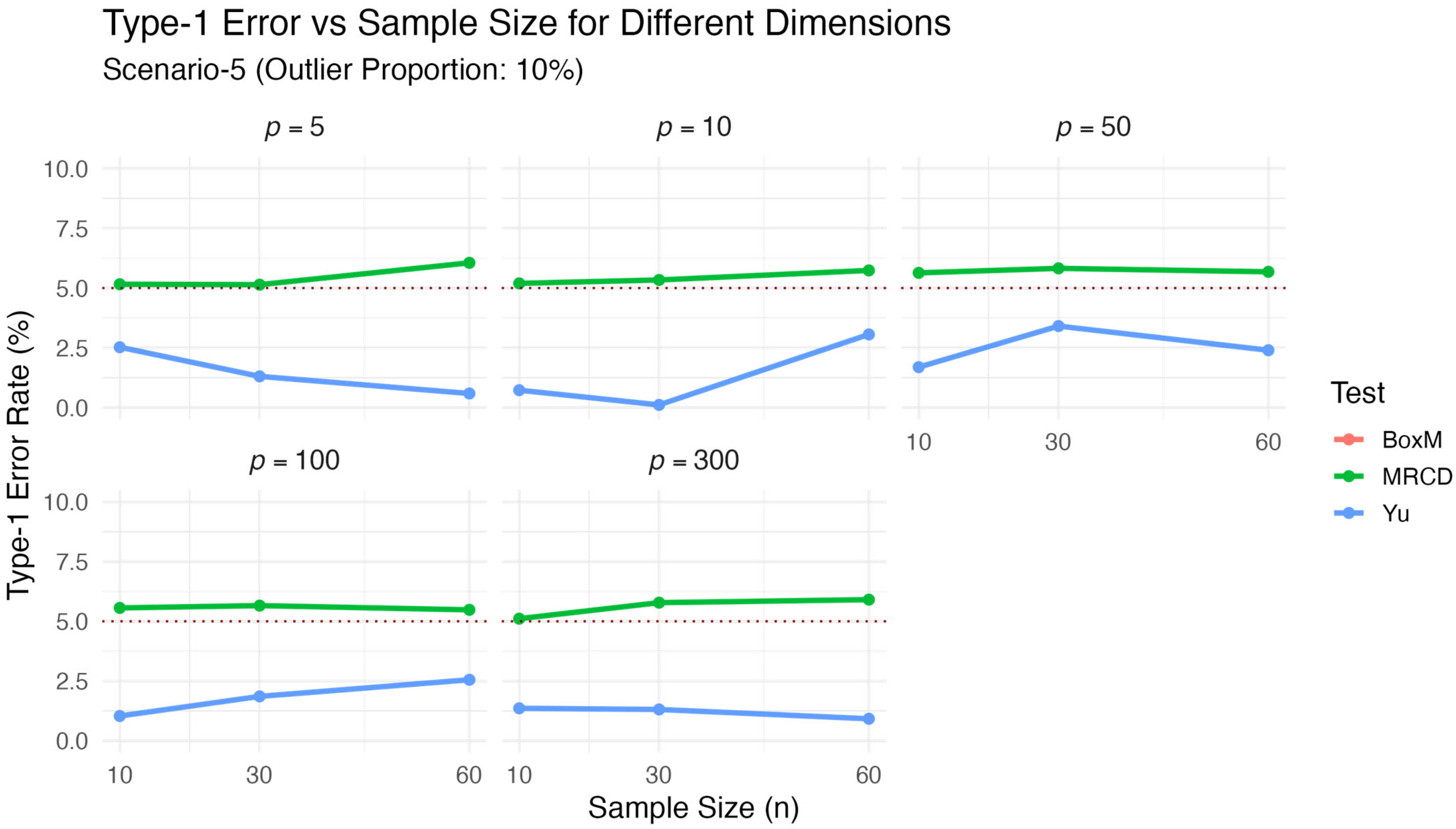
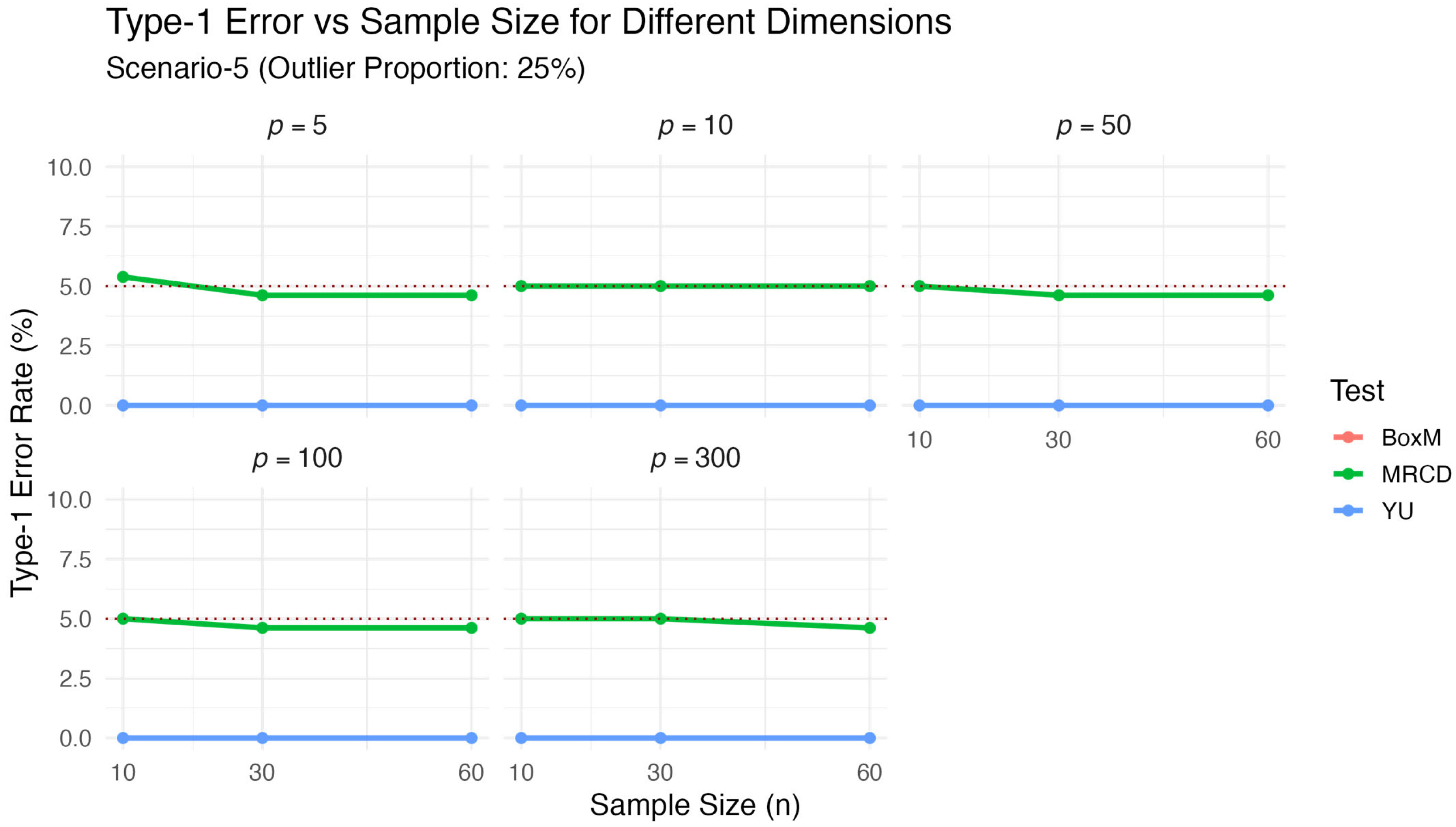
• Scenario 5: We generated datasets from a multivariate normal distribution. To generate regular observations, we set the mean vectors as ${\mu }_1={\mu }_2={\mu }_3=0$ without any loss of generality. Accordingly, regular observations in each group were randomly generated from $X_h~N_p\left({\mu }_h,{\Sigma }_h\right) \left(h=1,2,3\right)$. The proportion of regular observations in the data was $100-\phi$, where $\phi$ denotes the contamination rate. In Scenario 5, we used $\phi =10$ and 25 for sensitivity analysis. Outliers were generated from multivariate normal distributions $X_{h.out}~N_p\left({\mu }_{h.out},{\Sigma }_h\right) \left(h=1,2,3\right)$, with the following group-specific mean vectors:

$${\mu }_{1.out}={\left[log\left(p\right)\right]}_{p\times 1}, {\mu }_{2.out}={\left[-\sqrt{p}\right]}_{p\times 1}, {\mu }_{3.out}={\left[p\right]}_{p\times 1}$$

Although the mean vectors of the outliers differed among the groups, the covariance matrices remained identical, ensuring that the null hypothesis remained true even under contamination. Finally, we tested the null hypothesis $H_0:{\Sigma }_1={\Sigma }_2={\Sigma }_3,$ which holds in reality. The results for $\phi =10$ are presented in

Table 5. Robustness of methods based on normally distributed data with 10% contamination.

${\mathit{n}}_{\mathit{h}}$	p	$\mathit{T}{\mathit{M}}_{\mathit{M}\mathit{R}\mathit{C}\mathit{D}}$	$\mathit{T}{\mathit{M}}_{\mathit{Y}\mathit{U}}$	$\mathit{M}$
10	5	5.158	2.526	33.233
30	5	5.141	1.307	30.133
60	5	6.054	0.591	30.700
10	10	5.194	0.729	-
30	10	5.337	0.113	30.900
60	10	5.736	3.060	30.667
10	50	5.634	1.692	-
30	50	5.823	3.409	-
60	50	5.679	2.399	31.167
10	100	5.561	1.035	-
30	100	5.657	1.857	-
60	100	5.481	2.553	-
10	300	5.110	1.358	-
30	300	5.780	1.310	-
60	300	5.907	0.920	-
ARE:		11.002	66.855	522.667

and visualized in Figure 5. Similarly, the results for $\phi =25$ are presented in

Table 6. Robustness of methods based on contaminated normal distributed data with 25% contamination.

${\mathit{n}}_{\mathit{h}}$	p	$\mathit{T}{\mathit{M}}_{\mathit{M}\mathit{R}\mathit{C}\mathit{D}}$	$\mathit{T}{\mathit{M}}_{\mathit{Y}\mathit{U}}$	$\mathit{M}$
10	5	5.385	0.000	31.133
30	5	4.615	0.000	31.633
60	5	4.615	0.000	31.733
10	10	5.000	0.000	-
30	10	5.000	0.000	30.967
60	10	5.000	0.000	30.400
10	50	5.000	0.000	-
30	50	4.615	0.000	-
60	50	4.615	0.000	30.867
10	100	5.000	0.000	-
30	100	4.615	0.000	-
60	100	4.615	0.000	-
10	300	5.000	0.000	-
30	300	5.000	0.000	-
60	300	4.615	0.000	-
ARE:		4.103	100.000	672.444

and visualized in Figure 6.

The results of Scenario 5 given in Table 5 and Table 6 and visualized Figure 5 and Figure 6, explore the sensitivity of the test statistics to outlier contamination by comparing the results obtained under 10% and 25% contamination levels. When benchmarked against the clean data scenario (Scenario 1; Table 1 and Figure 1), a clear pattern emerges: as the proportion of contamination increased, the performance of the classical Box’s M and $T{M}_{YU}$ tests deteriorated significantly, while the proposed $T{M}_{MRCD}$ test remained stable. Specifically, under 10% contamination, Box’s M exhibited severely inflated type-1 error rates (ARE = 522.667), and $T{M}_{YU}$ also showed poor robustness (ARE = 66.855). This effect became even more pronounced under 25% contamination, where Box’s M failed entirely (ARE = 672.444) and $T{M}_{YU}$ consistently returned zero p-values, indicating excessive conservatism or breakdown. In contrast, $T{M}_{MRCD}$ maintained type-1 error rates remarkably close to the nominal 5% level across all contamination levels, with decreasing ARE values as contamination increased (11.002 at 10% vs. 4.103 at 25%). This stable performance under increasing contamination levels confirms that the MRCD estimator is effective in identifying and limiting the impact of outliers. Overall, the results clearly demonstrate that the proposed $T{M}_{MRCD}$ test provided strong robustness and reliability when the data included outliers.

• Scenario 6: All observation values in this scenario were initially generated as described in Scenario 2. To contaminate the data, we modified the last observation vector in each group: the last observation in group 1 was multiplied by −5, in group 2 by 5, and in group 3 by 15. This approach introduced group-specific outliers of varying magnitude, which resulted in different contamination rates depending on the group sample sizes. Importantly, the null hypothesis ${\mathrm{H}}_0:{\Sigma }_1={\Sigma }_2={\Sigma }_3$ remained valid in this setting. The impact of these structured outliers on the performance of the test statistics was evaluated, and the results are presented in

  Table 7. Robustness of methods based on mixed distributed data.

  ${\mathit{n}}_{\mathit{h}}$	p	$\mathit{T}{\mathit{M}}_{\mathit{M}\mathit{R}\mathit{C}\mathit{D}}$	$\mathit{T}{\mathit{M}}_{\mathit{Y}\mathit{U}}$	$\mathit{M}$
  10	5	5.292	0.013	99.193
  30	5	5.315	3.468	98.678
  60	5	5.230	0.464	99.137
  10	10	4.652	1.518	-
  30	10	5.220	0.623	99.315
  60	10	5.313	2.818	99.748
  10	50	5.212	0.400	-
  30	50	5.226	6.973	-
  60	50	5.256	0.913	99.603
  10	100	4.784	0.449	-
  30	100	5.208	0.713	-
  60	100	5.267	0.439	-
  10	300	5.305	0.673	-
  30	300	4.665	0.807	-
  60	300	5.399	0.486	-
  ARE:		5.522	77.585	1885.582

  and Figure 7.

Table 7 and Figure 7 present the robustness performance of the test statistics under Scenario 6, in which structured outliers of varying magnitude were introduced to each group. As expected, the proposed $T{M}_{MRCD}$ test maintained type-1 error rates close to the nominal 5% level across all combinations of n and p. This stability is confirmed by the lowest ARE value (5.522) among the three methods. In contrast, $T{M}_{YU}$ displayed substantial variability and inflated rejection rates, particularly for small sample sizes and moderate dimensional settings. The classical Box’s M test was severely affected by the contamination, with type-1 error rates exceeding 98% in nearly all configurations, yielding an extremely large ARE value of 1885.582. These findings confirm that the $T{M}_{MRCD}$ test is highly robust to structured outliers, whereas both $T{M}_{YU}$ and Box’s M failed to provide reliable control over the type-1 error under contaminated conditions.

6. Real Data Example

In this section, as in the simulation study, we analyze a real dataset to compare the performance of the proposed test statistic with the $T{M}_{YU}$ statistic proposed by Yu [7]. In this scenario, we used the dataset available at the NCBI website under the code GSE57275. This dataset includes 14 observations and 45281 genes (variables). In addition, these 14 observations are divided into three different groups.

These groups are called the controlled, infected, and infected-medication groups. The infected group consists of chips GSM1378192, GSM1378193, GSM1378194, and GSM1378195, resulting in a total of four observations in the first group. The infected-medication group consists of chips GSM1378196, GSM1378197, GSM1378198, GSM1378199, and GSM1378200. Finally, the control group consists of chips GSM1378201, GSM1378202, GSM1378203, GSM1378204, and GSM1378205. Therefore, there were five observations in both the second and third groups.

We tested whether the covariance matrices of these high-dimensional groups were equal or not and compared the test statistics. For this purpose, we also examined how the test statistics were affected as the $p/n$ ratio increased by determining different gene (variable) numbers. For this purpose, p values were chosen as 5, 20, 100, 300, 400, and 500. At all stages, the first p genes in the data were selected.

To examine the sensitivity of the test statistics to outliers, after performing the test process for clean data, we multiplied the last observation row in the first (infected) group by 10 and repeated this test process by creating an outlier in the dataset. Thus, we can see whether this outlier changed the decision made by the test statistics. The results are given in

Table 8. Results of tests using real data examples.

Dimensions	Data	$\mathit{T}{\mathit{M}}_{\mathit{M}\mathit{R}\mathit{C}\mathit{D}}$		$\mathit{T}{\mathit{M}}_{\mathit{Y}\mathit{U}}$
		Test Statistics	p-Value	Test Statistics	p-Value
5	Clean	2.876	0.340	3.169	0.747
	Cont.	3.570	0.393	13.934	0.000
20	Clean	3.884	0.060	17.544	0.210
	Cont.	3.811	0.100	55.676	0.000
100	Clean	3.747	0.620	66.871	0.510
	Cont.	3.863	0.230	278.434	0.000
200	Clean	3.879	0.260	135.704	0.470
	Cont.	3.966	0.051	556.622	0.000
300	Clean	3.872	0.260	208.216	0.380
	Cont.	3.967	0.060	834.640	0.000
400	Clean	3.871	0.500	277.074	0.410
	Cont.	3.971	0.070	1111.947	0.000
500	Clean	3.875	0.530	340.932	0.290
	Cont.	3.979	0.070	1390.207	0.000

.

According to Table 8, the $T{M}_{YU}$ and $T{M}_{MRCD}$ statistics failed to reject the null hypothesis $H_0:{\Sigma }_1={\Sigma }_2={\Sigma }_3$ when there were no outliers in the data $(p-\mathrm{values}>0.05)$. The $T{M}_{YU}$ statistic, however, rejected the null hypothesis when we added outliers to the data $(p-\mathrm{value}<0.001)$. Accordingly, it is concluded that the outliers in the data changed the decision of the $T{M}_{YU}$ statistic, indicating that this statistic is sensitive to outliers in data. On the other hand, the $T{M}_{MRCD}$ statistic still failed to reject data contaminated with outliers. Therefore, we can say that the outliers in the data had no effect on the decision of the $T{M}_{MRCD}$ statistic and that this statistic is robust to outliers.

7. Software Availability

We constructed the function RobPer_CovTest() in the R package entitled “MVTests” to perform the proposed robust permutational test on real datasets. This function needs four arguments: The data matrix is assigned to the argument x, and the grouping vector of observations is assigned to the argument group. The permutation number is assigned to the argument N (default of N = 100). Finally, the argument alpha, which takes a value between 0.5 and 1 (default of alpha = 0.75), can be used to determine the trimming parameter. The function obtains the p-value, the $T{M}_{MRCD}$ value, and the $T{M}_{MRCD}^{\left(r\right)} \left(r=1,2,\dots ,N\right)$ values. Due to this function, all researchers can use our proposed test statistics without being affected by outliers to compare covariance matrices in high-dimensional data. Researchers can install this package from GitHub by using the following code block:

install.packages(“devtools”)

devtools::install_github(“hsnbulut/MVTests”)

8. Conclusions

Classical methods cannot be used to test the equality of covariance matrices in high-dimensional settings because the classical covariance matrix becomes singular, making its determinant zero and inverse undefined. Several alternative methods have been proposed in the literature to address this problem, as summarized in Section 2. However, these proposed tests are used for high-dimensional data, they are not robust to outliers in the data. To overcome this limitation, this study proposes a new test statistic, $T{M}_{MRCD}$, designed to compare covariance matrices in high-dimensional data while being resistant to outlier effects.

The performance of the proposed test was evaluated through an extensive simulation study focusing on its type-1 error control, statistical power, and robustness. In the simulation study, it was observed that the proposed approach had a lower ARE value in terms of type-1 than the $T{M}_{YU}$ statistic proposed by Yu [7]. Accordingly, it can be said that the proposed approach is more successful in terms of type-1 error rate. Although $T{M}_{YU}$ exhibited higher statistical power, $T{M}_{MRCD}$ remained competitive. Importantly, the robustness comparisons reveal that $T{M}_{MRCD}$ maintained a low ARE under contamination while the $T{M}_{YU}$ statistic became highly sensitive to outliers and yielded inflated rejection rates.

Although $T{M}_{MRCD}$ does not permit closed-form distribution under the null or alternative hypotheses due to its permutation-based structure, its asymptotic consistency can be justified empirically and theoretically. Under the null hypothesis, permutation-based tests are known to control the type-1 error asymptotically [17]. Under the alternative hypothesis, the proposed test statistic diverged from its permutation distribution as the group differences in covariance increased, thereby leading to the power converging to 1 as the sample size increased. This behavior is supported by the simulation results reported in Table 1, Table 2, Table 3 and Table 4.

To further compare their practical performance, we applied both test statistics to a real gene expression dataset. In these analyses, both the $T{M}_{YU}$ and $T{M}_{MRCD}$ statistics failed to reject the null hypothesis on clean data. However, when the data were contaminated, the $T{M}_{YU}$ statistic no longer failed to reject the null hypothesis, while $T{M}_{MRCD}$ maintained the same decision without being affected by the outliers. This real data example shows that the proposed test can be used on high-dimensional data without being affected by outliers. For a concise summary of the key differences among the proposed test $T{M}_{MRCD}$, the $T{M}_{YU}$ statistic, and Box’s M test, we refer the reader to the comparative table provided in

Table A2. Comparison of test statistics.

Test	Robust to Outliers	High-Dimensional Applicability (p > n)	Estimation Approach
$Box\prime s M$	No	No	Classical covariance
$T{M}_{YU}$	No	Yes	Classical covariance + permutation
$T{M}_{MRCD}$	Yes	Yes	MRCD estimators + permutation

in Appendix A.

Finally, to support real-world applications, we implemented the proposed test as an R function in the MVTests package. In conclusion, we believe that the proposed approach can contribute to the literature not only theoretically but also practically.